Submitted:
29 May 2024
Posted:
30 May 2024
You are already at the latest version
Abstract
Using two independent speckle imaging systems based on the recently published LSOCI method operating in contact mode on the skin, we assess the reproducibility of in vivo measurements and conduct an inter-instrument comparison. To this aim, we propose a calibration method to handle each imaging system as a comprehensive unit, which includes the laser source, optics, and camera. Our experimental results demonstrate that the microcirculation images produced by both instruments exhibit high accuracy and stability, with microcirculation activity values in excellent agreement, thereby paving the way for clinical applications.
Keywords:
microcirculation
; in vivo imaging
; calibration
; dynamic speckle
; vascularization
; LSOCI
1. Introduction
Dynamic speckle imaging represents a highly promising tool for observing microcirculation, which plays a crucial role in delivering nutrients and oxygen to billions of cells with each heartbeat. Alterations in microcirculation are associated with various pathologies, such as cancer [1], diabetes [2,3], hypertension [4], sepsis [5], and viral infections [6].
This field is still very much alive, as witnessed by the new publications on the influence of microcirculation in various pathologies [7], including Covid [8], and the renewed interest in the associated dynamic speckle technology [9,10,11].
Therefore, monitoring the peripheral microcirculation of the body holds significant diagnostic potential.
Since the pioneering work by Briers [12], numerous advancements have been made in both the qualitative and quantitative analysis of blood circulation and microcirculation through dynamic speckle imaging.
Recently, our team developed an additional modality to the established Laser Speckle Contrast Imaging (LSCI) method, called Laser Speckle Orthogonal Contrast Imaging (LSOCI) [13]. This technique represents a polarimetric enhancement of traditional laser speckle imaging methodologies, such as laser speckle contrast analysis [12] and laser speckle contrast imaging [14].
LSOCI is based on the polarimetric selection of spatially depolarized scattered fields, primarily driven by the motion of red blood cells. In practice, when the skin is illuminated with a fully polarized laser in the near-infrared spectrum, we observe two principal contributions of backscattered light: one from the skin surface, which can be considered rough at the wavelength scale and that largely conserves the incident polarization, and another emanating from deeper layers, that has undergone multiple scattering events, resulting in random polarization [15]. Both scattering sources contribute to the speckle pattern, but the surface-generated contribution can be effectively eliminated using a polarizer aligned orthogonally to the polarimetric state of the illuminating laser. This selective filtering leaves primarily the multi-scattered photons from deeper layers, which are especially sensitive to micro-movements.
By employing such a polarimetric filtering system with orthogonal states, we have successfully captured new images of microcirculation at an estimated depth of approximately 3 mm on the face. This interesting depth is achieved through the use of both the strongly penetrating near-infrared wavelength and the polarimetric selection of multiple scattering events. Additionally, when the device is in contact with the skin, a spatial resolution of 80 m has been achieved. This is made possible by significantly reducing the relative movement between the imaging system and the observed area during the acquisition time[13].
However, overcoming the challenges of adapting this technology for clinical use in pathology detection and diagnostics requires addressing several critical constraints:
- Quantified Indices per Pixel: Each pixel in the image should provide a quantified index of microcirculation activity, essential for informing and guiding treatment decisions.
- Stability in Repeated Acquisitions: When imaging the same area with the body at rest, the technology must produce consistently stable images and microcirculation activity values.
- Inter-Instrument Consistency: Results must be comparable across different imaging systems.
- Dynamic and Accurate Imaging: The imaging system must exhibit sufficient dynamic range, stability, and accuracy to distinguish between different pathological states, despite challenges posed by in vivo conditions such as the cardiac cycle and unavoidable movements.
From a practical standpoint—essential for practitioners—the imaging systems should be compact, lightweight, portable, and quick to deploy. This article aims to address all these points comprehensively.
To this end, we have developed two lightweight and compact imaging systems utilizing the LSOCI method. In this paper, we present results regarding the dynamics, stability, and accuracy of measurements from each apparatus, along with a comparative analysis between the two systems. We discuss the conditions necessary for an effective comparison within the framework of a global calibration method specifically elaborated for dynamic speckle imaging.
We first propose to compare both instruments from the perspective of the displayed contrast in highly detailed microcirculation structures. To meet this requirement, we performed a minor scratch on the skin, which revealed significant spatial details.
Then, to associate each camera pixel with a reliable and comparable microcirculation value between both instruments, we use a global calibration method. This latter was developed based on the understanding that the physical signal carrying biophysical information is not the absolute measurement of spatial or temporal speckle contrast, but rather a deviation of these contrasts from a reference value, which depends on each imaging system as a whole.
Finally, utilizing this calibration procedure, we conduct a quantitative comparison between the two instruments. Despite the extensive research into dynamic speckle imaging since the 1980s, to our knowledge, this study presents the first qualitative and quantitative comparisons of two dynamic speckle imaging instruments scanning the same in vivo area.
2. Materials and Methods
2.1. Experimental Setup
Two Laser Speckle Orthogonal Contrast Imaging instruments, namely LSOCI1 and LSOCI2, use a linearly polarized TEM00 mode laser (Lambdamini from RGB Photonics) with a central wavelength around 785 nm. Their laser beam is sent through some diverging optics to illuminate a skin surface of about . Backscattered photons are then filtered by a linear grid polarizer (THO-WP25M-UB from Thorlabs) in which the eigenaxis is set orthogonal to the polarization state of the laser illumination, before reaching a monochrome CMOS camera of 1.5 million pixels (aca1440-220um from Basler), according to our previously published article [13]. LSOCI1 and LSOCI2 emit, due to different diverging optics and laser power, respectively 14 and 7.5 on the skin surface. Moreover, their cameras are set to have different numerical apertures which results in a ratio of approximately 2 between their speckle grain size, with a similar detected mean intensity. All microcirculation images are calculated from the temporal contrast of 200 raw intensity images with 12ms integration time each. Both systems are used in contact with the skin in order to minimize movements during acquisitions.
2.2. Contrast Variation Calibration Method (CVCM)
The common calibration procedures used [16,17,18] for absolute flow measurements within the framework of dynamic speckle imaging are primarily based on the experimental determination of the coefficient. This parameter stems from Siegert’s relation [19,20], which links the intensity temporal auto-correlation function to the electric field correlation function. Experimentally, the coefficient is expected to reflect the spectral characteristics of the laser source, polarization effects, and the spatial and temporal averaging of the speckle on the camera. This implicitly includes the coherence effects and the mismatch between the speckle grain size (determined by the intensity autocorrelation function [21]) and the pixel size.
However, these powerful calibration procedures appear more suited to research activities than clinical use due to their complex implementation. Furthermore, temporary perturbations in the imaging instrument, such as those due to temperature variations or optical re-injection affecting the laser source characteristics, could go undetected and potentially yield inconsistent results. Therefore, a near-instantaneous calibration method would be beneficial to verify the consistency and stability of the entire imaging system, even though it may only support semi-quantitative results. We have observed that in several recent articles, was arbitrarily set to 1; however, in our case, such simplification would hinder comparisons between instruments. Thus, we propose a straightforward method called the Contrast Variation Calibration Method (CVCM), which allows for near-instantaneous calibration and thereby allows inter-instrument comparison.
Before going deeper into this method, it is important to highlight an intrinsic limitation of our imaging system regarding absolute blood flow measurements: since we rely on multi-scattered photons to generate our signal, we characterize more the activity of microcirculation rather than the absolute linear velocity of blood cells. By activity, we refer to the overall agitation of blood cells in potentially all three spatial dimensions, without specifying which direction predominates in general cases. Thus, using the LSOCI method, the introduced in [13] describes how rapidly a global agitation of blood cells, through multiple scattering, leads to speckle decorrelation. An analogy for the in the context of microcirculation in blood vessels could be the state variable of temperature, which characterizes the agitation and average speed of molecules or atoms in a confined gas. Ultimately, the LSOCI method offers enhanced penetration depth and greater sensitivity to the movement of blood cells due to its reliance on exclusive multiple scattering detection. However, it generally does not allow absolute speed measurements. Therefore, the goal here is to provide guidelines for performing stable, accurate, and comparable semi-quantitative measurements between LSOCI instruments.
2.3. Equation for Normalized VMAI
In previous studies [13,22,23], it was inferred that under both hypotheses of a Lorentzian and Gaussian distribution for the speed of red blood cells, the decorrelation time of the speckle pattern can be expressed as , where T is the integration time of the camera, and denotes the observed contrast in the polarimetric orthogonal configuration between the laser illumination and the polarizer in the detection arm. The Volume Microcirculation Activity Index (VMAI) was defined as the inverse of this decorrelation time, in accordance with the previously defined Blood Flow Index definition [24], resulting in the following equation:
While this equation can be used to assess the general trend of microcirculatory activity, it is not sufficient for performing inter-instrument comparisons. Firstly, we observe that for a spatial contrast of 1, theoretically achievable using a static scatterer generating a circular Gaussian speckle, such a definition of the introduces an offset value of , which must be removed to meet the correct boundary conditions. Secondly, we suggest that the should tend to infinity as the agitation reaches its maximum and thus decreases the contrast to 0, assuming there is no static scatterer present. Consequently, we propose the following empirical equation for the normalized , denoted as , in Equation 2. This formulation: 1) retains the dependence, 2) eliminates the offset value of when , and 3) normalizes the observed contrast using a reference contrast value :
with .
represents the maximum speckle contrast achievable on a reference static scatterer using the entire imaging system. This value characterizes the complete imaging setup, encompassing the spectral width of the laser, its polarization properties, and the camera’s numerical aperture and pixel density.
This maximum value is experimentally determined by illuminating a reference scatterer that produces a circular Gaussian speckle [25,26]. Therefore, the standard deviation of the surface height distribution of this reference scatterer should be at least on the order of the laser wavelength, and the illumination diameter must encompass a sufficient number of roughness correlation cells. Microcirculation activity is then quantified based on deviations of the spatial contrast from this maximum value. Additionally, under the ergodic hypothesis, is also considered the highest achievable temporal speckle contrast, thus allowing similar treatments as the spatial contrast.
3. Results
3.1. Qualitative Inter-Instrument Comparison for Temporal Speckle Contrast Images
The contact mode used in the LSOCI method effectively minimizes relative movements between the instrument head and the observed area, revealing high spatial details. These details are especially pronounced in images of microcirculation activity within irritated skin areas. Additionally, we noted a notable variability in the measurement of microcirculation activity on both the face and hands, influenced by environmental temperature variations. Consequently, we opted to induce a mild irritation on the belly just below a naevus. Both instruments LSOCI1 and LSOCI2, were used to capture images of the same area before and after the irritation was mechanically induced. To ensure a thorough comparison, both instruments were alternated and repositioned after each acquisition, tracking the entire temporal evolution of the skin’s reaction.
We first illustrate the area that received the scratch in Figure 1. Panel (a) features a red dotted line that precisely indicates the future location of the scratch, and panel (b) highlights the faint red irritated area that was barely visible to the naked eye after the scratch.
Figure 2 displays 12 sample images out of the 54 acquisitions performed by both instruments. A pronounced skin reaction is clearly observed in the .
Despite the challenges posed by in vivo conditions, including inevitable movements and the effects of the heartbeat cycle over the acquisition time, both instruments exhibit very similar patterns. It is noted that the heartbeat cycle is only partially averaged, even though the total acquisition time is 200x12ms=2,4s. Variations in the onset of acquisition relative to the systolic phase of the heartbeat contribute to a non-negligible random contribution across different acquisitions. In live mode, our imaging systems clearly display the heart’s pulsation within the angioma.
The third column of Figure 2 shows a significant reaction in the area surrounding the injury, which markedly increases its blood circulation. This reaction pattern appeared almost immediately after the scratch (<1s). Generally speaking, both instruments provide very similar pre- and post-injury images throughout the healing process, the last column relating the microcirculation 4h and 25 minutes after the scratch.
As illustrated in Figure 3, common circled details can be observed by both instruments, the smaller one (circled in green) measuring less than 1 mm (4 pixels). Note that the spatial resolution of our imaging systems is determined by the optics and pixel density of the camera; while it can be significantly improved, this enhancement comes at the cost of a smaller field of view.
As pointed out earlier, these acquisitions were performed by constantly removing and quickly replacing each instrument on the same area, positioned at roughly a angle relative to the surface of the skin. Therefore, the image stability observed in both instruments represents a very promising result in terms of operator dependency.
3.2. Quantitative Inter-Instrument Comparison for Temporal Speckle Contrast Images
3.2.1. Contrast Linearity Domain
Before discussing the experimental results of in vivo measurements, it is important to note that a fully or nearly fully developed speckle pattern, composed of very dark and very bright spots, challenges the linearity of the camera due to its highly contrasted structure. Specifically, we aim to characterize the linearity domain of our cameras in terms of the stability of the temporal contrast. This involves determining the range with the corresponding error, within which the temporal contrast remains primarily stable as the received intensity (or numerical counts, NC) increases.
Figure 4 (a) illustrates the evolution of histograms from left to right when illuminating a white paper sheet (Canson paper, , previously characterized by polarimetry in ref.[15]) with increasing detection integration times. Between the regimes of too low and too high numerical counts, where respectively dark noise and camera saturation predominate, we can identify an acceptable domain of linearity (highlighted in green in (b)), within which the variation of the contrast is less than 0.01. Therefore, all acquisitions must utilize speckle patterns with histograms falling within this linearity domain for measurements, to avoid the need of error compensation.
3.2.2. Measurements and Analysis between Two LSOCI Instruments
As previously mentioned, both imaging systems LSOCI1 and LSOCI2 don’t have the same diverging optics and laser power. Thus, in order to work inside the contrast linearity range of intensity previously described, the optical aperture of the cameras were used to compensate for the difference of energy received. LSOCI1 and LSOCI2 respectively emitted and onto the skin, but their respective camera apertures were set to achieve both an average numerical count corresponding to the middle of the contrast linearity range, highlighted in green in Figure 4 (b). Consequently, this led to a difference in the speckle grain size ratio of approximately 2 between the two imaging systems, with the smaller grain size of LSOCI2 characterized by approximately 2 pixels. This disparity in speckle grain size resulted in different values between the two instruments when illuminating the reference static sample.
For each of the 54 acquisitions performed (27 for each instrument), the values were recorded, resulting in mean values of 0.70 and 0.67 with associated standard deviations of 0.016 and 0.014 for LSOCI1 and LSOCI2 respectively, after camera linearization and shot noise removal. It is noteworthy that the spectral characteristics of lasers used in dynamic speckle imaging have only recently been addressed [27], despite their significant impact on the value through their spectral width. In this experiment, the lasers were not temperature stabilized, and occasional mode hops could change this reference value, necessitating its update before each acquisition. However, with temperature stabilized single longitudinal mode lasers, a single acquisition value of for each imaging system would likely suffice due to the stability of the longitudinal mode, thus rendering the CVCM calibration procedure particularly simple and nearly instantaneous.
Finally, utilizing a different and characteristic for both instruments enables us to replace the calibration procedure, while still maintaining the capability to perform semi-quantitative measurements, which are primarily required in clinical applications.
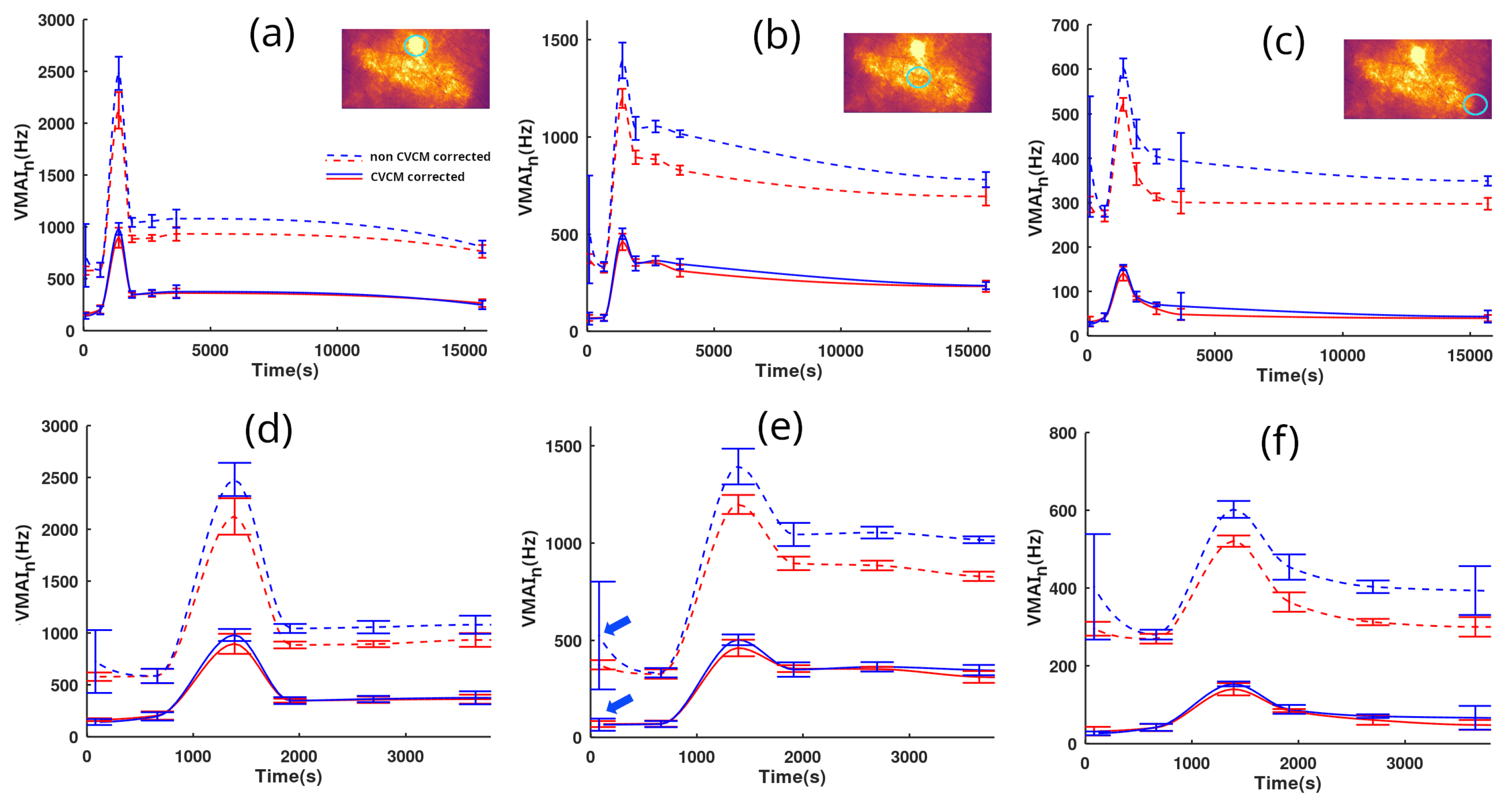
Figure 5 presents quantified observations of the microcirculation skin reaction. Time tracking was performed by both LSOCI1 and LSOCI2 instruments and lasted 4 hours and 25 minutes. Panels (a)(d), (b)(e), and (c)(f) correspond to selected regions of interest circled in green, respectively located on the angioma, the center of the scratch, and a more peripheral zone farther from the scratch. The objective was to test the CVCM throughout the entire dynamic range of the image. Panels (d), (e), and (f) are the temporal zooms of (a), (b), and (c) respectively. LSOCI1 and LSOCI2 are represented by red and blue colors, respectively. Dotted lines indicate the results obtained without calibration, setting to 1 for every acquisition, while solid lines utilize the correction according to the CVCM.
In order to partially average the cardiac cycle effect, each point on the curves was obtained by averaging at least three closely timed measurements for each instrument, while adhering to the previously described switch-and-replace procedure between acquisitions. The standard deviation for each group of closely timed acquisitions is represented by vertical bars.
An overall comment reveals that the non-corrected blue dotted curve of the LSOCI2 instrument consistently lies above the red ones. However, this offset is effectively corrected using the CVCM, for all values across the full range of acquisitions (between 20 and 1000 Hz).
Upon closer examination, as can be observed in panels (d), (e), and (f), the first group of closely timed acquisitions of LSOCI2 —indicated by blue arrows only in (e) for clarity— displays a surprisingly high mean value along with an abnormally high deviation in the non-corrected blue dotted line. Both values are noticeably different compared to the simultaneous LSOCI1 measurements and also to subsequent acquisitions performed by both instruments minutes later. Nevertheless, with the CVCM, both the abnormal mean and deviation values are corrected and align well with other measurements, as seen in the corresponding solid lines. This behavior is indicative of a laser mode hop that temporarily altered the value of LSOCI2. However, this variation was successfully detected and corrected using the acquisition on the static scatterer, according to the CVCM. From our experience, such mode hops in the lasers used in this experiment could change the value by up to 25%.
Finally, Despite the residual effects of the cardiac cycle and potential movements during acquisitions, the CVCM successfully harmonized all the acquisitions performed by both instruments, as demonstrated by the excellent overlay of the full blue and red lines.
4. Conclusion and Perspectives
To enable a quantified comparison between two distinct LSOCI instruments, we’ve proposed the near real-time Contrast Variation Calibration Method, which characterizes each dynamic speckle imaging system as a comprehensive unit, encompassing the laser source, optics, and camera. This approach utilizes a unique parameter of calibration for each instrument which is the maximum spatial contrast, attainable under given acquisition parameters, while imaging a static scatterer producing a circular Gaussian speckle field. The microcirculation activity is then reached through the deviation, whether in temporal or spatial contrast, from this maximum value in response to the agitation of red blood cells. Using this calibration method, we have followed in time the evolution of a scratch on the belly using 2 similar LSOCI instruments, but with different laser power, optics and detection apertures. Microcirculation patterns and measures are in excellent agreement between both imaging systems. Thus, despite being limited to semi-quantitative measurements, the LSOCI method with CVCM provides a high dynamic range, accuracy, and stability of the signal, which can moreover be successfully compared between calibrated instruments. We believe that these results are particularly promising for numerous medical applications such as real-time monitoring of tumor evolution under therapy, accurate characterization of diabetes stage assessment, various surgical applications, and the evaluation of burn evolution. However, further improvements can be performed. Especially, the validity domain of this calibration method should be studied regarding various numerical apertures and laser spectral widths. Moreover, the sensitivity of the signal regarding the chosen integration time in function of the observed dynamic of red blood cells should be carefully addressed to be further optimized.
Author Contributions
This work has been led with Financial Support from ITMO Cancer AVIESAN (Alliance Nationale pour les Sciences de la Vie et de la Santé, National Alliance for Life Sciences & Health) within the framework of the Cancer Plan (Under Contract No. 18CP112-00.
Funding
All the authors have contributed equally to the work.
References
- Stücker, M.; Horstmann, I.; Röchling, A.; Hoffmann, K.; Nüchel, C.; Altmeyer, P. Differential diagnosis of skin tumors using tumor microcirculation. In Skin Cancer and UV Radiation; Springer, 1997; pp. 999–1006.
- Li, J.; Cao, Y.; Liu, W.; Wang, Q.; Qian, Y.; Lu, P. Correlations among diabetic microvascular complications: a systematic review and meta-analysis. Scientific Reports 2019, 9, 3137. [CrossRef]
- Strain, W.D.; Paldánius, P. Diabetes, cardiovascular disease and the microcirculation. Cardiovascular diabetology 2018, 17, 1–10. [CrossRef]
- Lara Rezende, G.; da Silva, M.d.G.; Soares Takano, G.H.; Lopes Sampaio, A.L.; Oliveira Soares, R.; dos Santos Kückelhaus, C.; Souza Kückelhaus, S.A. Hypertension causes structural lesions in the microvasculature of the posterior nasal mucosa. Hypertension Research 2021, 44, 591–594. [CrossRef]
- De Backer, D.; Creteur, J.; Preiser, J.C.; Dubois, M.J.; Vincent, J.L. Microvascular blood flow is altered in patients with sepsis. American journal of respiratory and critical care medicine 2002, 166, 98–104. [CrossRef]
- Damiani, E.; Carsetti, A.; Casarotta, E.; Scorcella, C.; Domizi, R.; Adrario, E.; Donati, A. Microvascular alterations in patients with SARS-COV-2 severe pneumonia. Annals of Intensive Care 2020, 10, 1–3. [CrossRef]
- Narzulaeva, U. Pathogenetic Mechanisms of Microcirculation disorders. International Bulletin of Medical Sciences and Clinical Research 2023, 3, 60–65.
- Zharkikh, E.V.; Loktionova, Y.I.; Fedorovich, A.A.; Gorshkov, A.Y.; Dunaev, A.V. Assessment of blood microcirculation changes after COVID-19 using wearable laser Doppler flowmetry. Diagnostics 2023, 13, 920. [CrossRef]
- Sdobnov, A.; Piavchenko, G.; Bykov, A.; Meglinski, I. Advances in dynamic light scattering imaging of blood flow. Laser & Photonics Reviews 2024, 18, 2300494.
- Ruan, Z.; Li, R.; Dong, W.; Cui, Z.; Yang, H.; Ren, R. Laser speckle contrast imaging to monitor microcirculation: An effective method to predict outcome in patients with sepsis and septic shock. Frontiers in Bioengineering and Biotechnology 2023, 10, 1067739. [CrossRef]
- Golubova, N.; Potapova, E.; Seryogina, E.; Dremin, V. Time–frequency analysis of laser speckle contrast for transcranial assessment of cerebral blood flow. Biomedical Signal Processing and Control 2023, 85, 104969. [CrossRef]
- Briers, J.D.; Webster, S. Laser speckle contrast analysis (LASCA): a nonscanning, full-field technique for monitoring capillary blood flow. Journal of biomedical optics 1996, 1, 174–179. [CrossRef]
- Colin, E.; Plyer, A.; Golzio, M.; Meyer, N.; Favre, G.; Orlik, X. Imaging of the skin microvascularization using spatially depolarized dynamic speckle. Journal of Biomedical Optics 2022, 27, 046003–046003. [CrossRef]
- Kirkpatrick, S.J.; Duncan, D.D.; Wells-Gray, E.M. Detrimental effects of speckle-pixel size matching in laser speckle contrast imaging. Optics letters 2008, 33, 2886–2888. [CrossRef]
- Dupont, J.; Orlik, X.; Ghabbach, A.; Zerrad, M.; Soriano, G.; Amra, C. Polarization analysis of speckle field below its transverse correlation width: application to surface and bulk scattering. Optics Express 2014, 22, 24133–24141. [CrossRef]
- Wang, C.; Cao, Z.; Jin, X.; Lin, W.; Zheng, Y.; Zeng, B.; Xu, M. Robust quantitative single-exposure laser speckle imaging with true flow speckle contrast in the temporal and spatial domains. Biomedical Optics Express 2019, 10, 4097–4114. [CrossRef]
- Liu, H.L.; Yuan, Y.; Han, L.; Bi, Y.; Yu, W.Y.; Yu, Y. Wide dynamic range measurement of blood flow in vivo using laser speckle contrast imaging. Journal of Biomedical Optics 2024, 29, 016009–016009. [CrossRef]
- Postnov, D.D.; Tang, J.; Erdener, S.E.; Kılıç, K.; Boas, D.A. Dynamic light scattering imaging. Science advances 2020, 6, eabc4628. [CrossRef]
- Fercher, A.; Briers, D. Flow visualization by means of single-exposure speckle photography. Optics Communications 1981, 37, 326–330. [CrossRef]
- Maret, G. Diffusing-wave spectroscopy. Current opinion in colloid & interface science 1997, 2, 251–257.
- Goldfischer, L.I. Autocorrelation function and power spectral density of laser-produced speckle patterns. Josa 1965, 55, 247–253. [CrossRef]
- Duncan, D.D.; Kirkpatrick, S.J. Can laser speckle flowmetry be made a quantitative tool? JOSA A 2008, 25, 2088–2094. [CrossRef]
- Ramirez-San-Juan, J.C.; Ramos-Garcia, R.; Guizar-Iturbide, I.; Martinez-Niconoff, G.; Choi, B. Impact of velocity distribution assumption on simplified laser speckle imaging equation. Optics express 2008, 16, 3197–3203. [CrossRef]
- Sunil, S.; Zilpelwar, S.; Boas, D.A.; Postnov, D.D. Guidelines for obtaining an absolute blood flow index with laser speckle contrast imaging. bioRxiv 2021, pp. 2021–04.
- Goodman, J.W. Statistical optics; John Wiley & Sons, 2015.
- Bergoënd, I.; Orlik, X.; Lacot, E. Study of a circular Gaussian transition in an optical speckle field. Journal of the European Optical Society-Rapid Publications 2008, 3. [CrossRef]
- Postnov, D.D.; Cheng, X.; Erdener, S.E.; Boas, D.A. Choosing a laser for laser speckle contrast imaging. Scientific reports 2019, 9, 2542. [CrossRef]
Figure 1.
(a) Image of the studied area with a red dotted line indicating the future location of the scratch, positioned just below a red angioma. (b) Image of the same area taken after the scratch, highlighting a faintly irritated red area that is barely visible to the naked eye, circled in red.
Figure 1.
(a) Image of the studied area with a red dotted line indicating the future location of the scratch, positioned just below a red angioma. (b) Image of the same area taken after the scratch, highlighting a faintly irritated red area that is barely visible to the naked eye, circled in red.
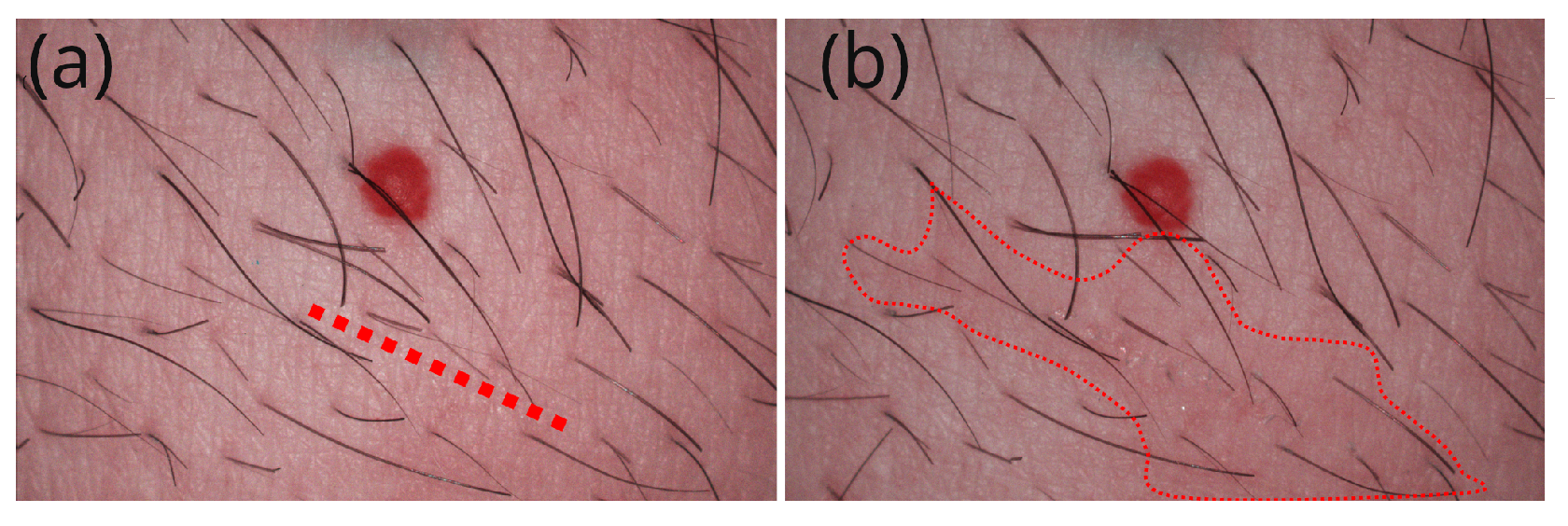
Figure 2.
Temporal evolution of a scratch on the belly beneath an angioma, followed by two LSOCI instruments that exhibit very similar microcirculation patterns.
Figure 2.
Temporal evolution of a scratch on the belly beneath an angioma, followed by two LSOCI instruments that exhibit very similar microcirculation patterns.
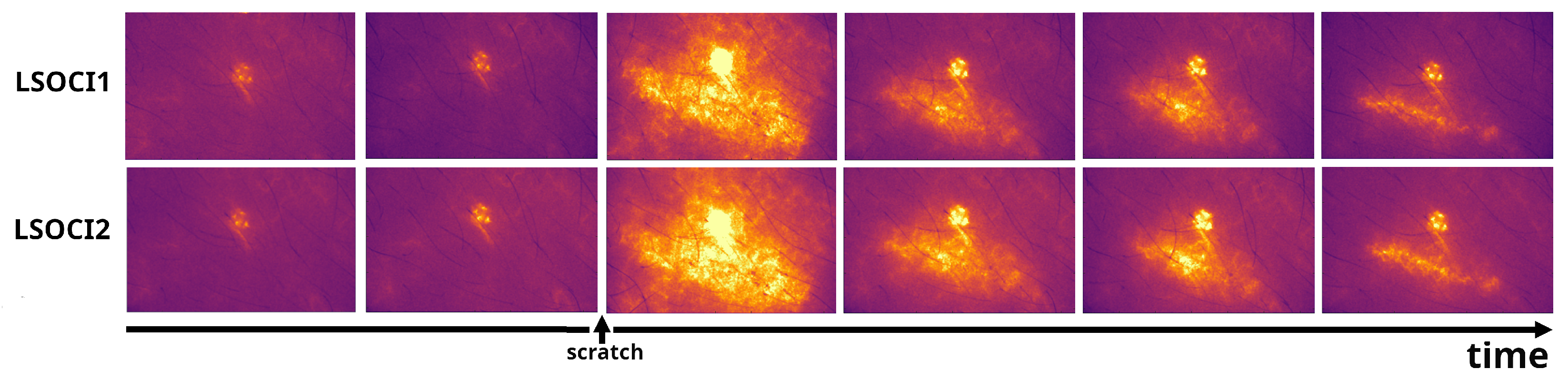
Figure 3.
A zoom into the more intense pattern observed in the previous figure reveals common spatial details, enclosed in circles. A submillimeter-sized detail (enclosed in green) can be observed.
Figure 3.
A zoom into the more intense pattern observed in the previous figure reveals common spatial details, enclosed in circles. A submillimeter-sized detail (enclosed in green) can be observed.
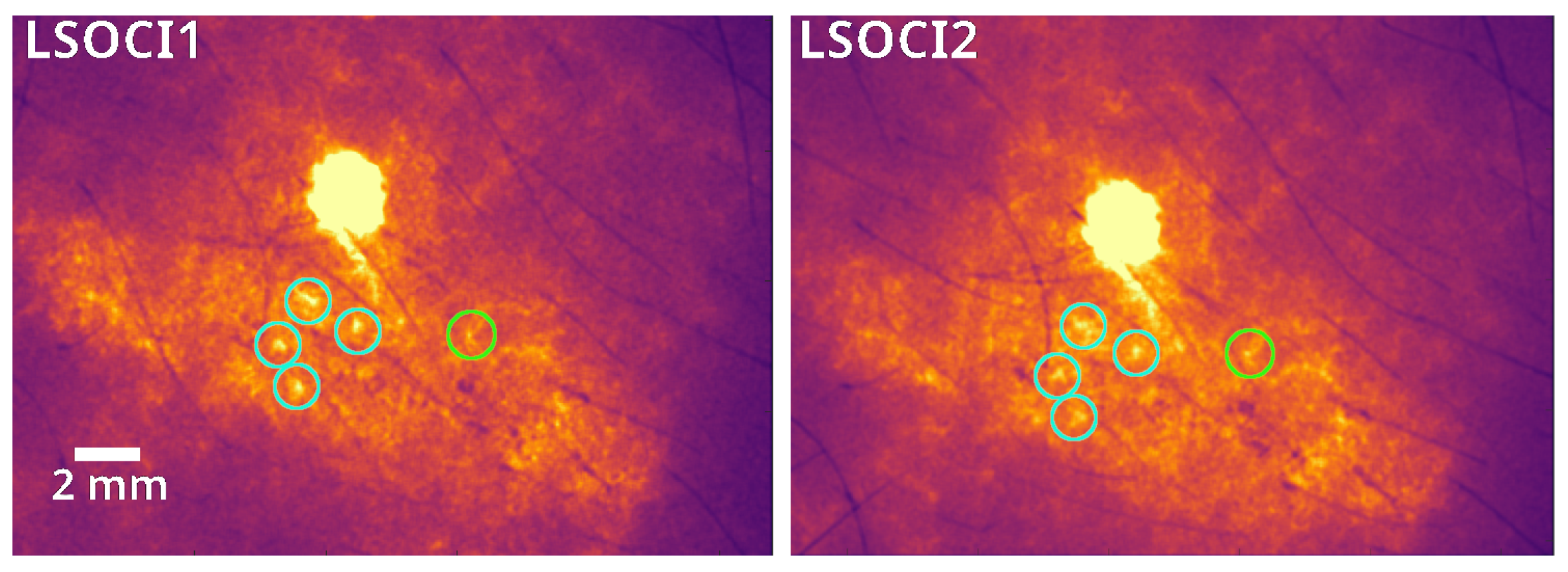
Figure 4.
(a) Experimental Circular Gaussian Speckle histograms and (b) associated spatial contrasts, as a function of the average numerical count (<NC>) of the camera. Three domains are clearly distinguished in (b): on the left, a regime with too low numerical counts corresponds to abnormally high spatial contrast; in the middle, a near-linear regime where the spatial contrast remains relatively stable with increasing <NC>; and on the right, a saturation regime that decreases the spatial contrast as the saturated fraction increases (indicated in red on (b)). We choose to operate within the near-linear regime, marked in green, where the contrast variation is less than 0.01.
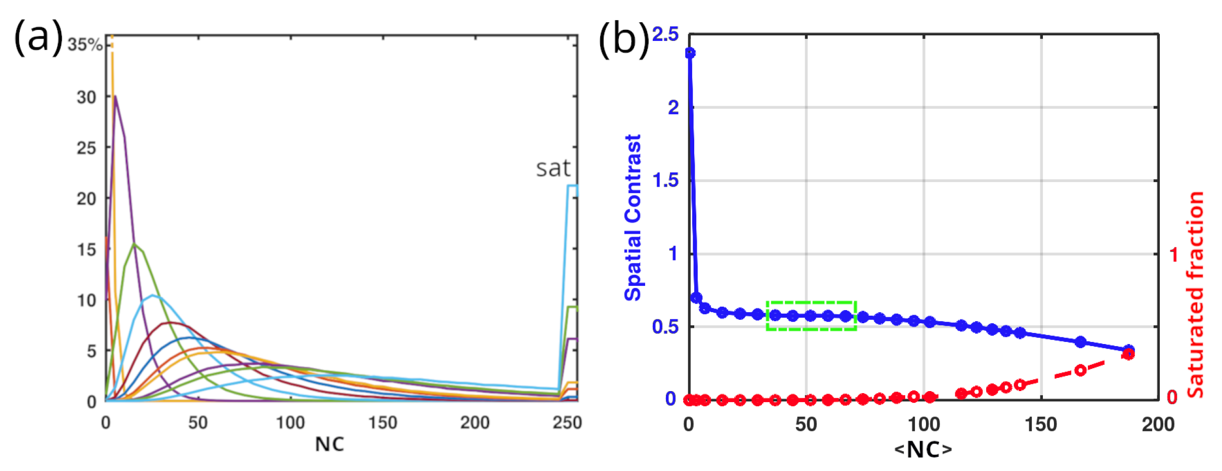
Figure 5.
measurements captured by two LSOCI instruments over time, before and after a scratch provoking an irritation. Measures from LSOCI1 and LSOCI2 are respectively represented in red and blue. Each column corresponds to the temporal study of the mean value over a region of interest circled in blue in the thumbnail images above. Panels (d), (e), and (f) are temporal zooms of panels (a), (b), and (c), respectively. Dotted lines represent measurements without calibration (), while solid lines reflect the CVCM correction with a distinct value measured for each acquisition. Despite only partial averaging of the cardiac cycle effect and unavoidable movements, the totality of the calibrated acquisitions from both LSOCI1 and LSOCI2 yield very similar results, in opposition to non-calibrated values shown in dotted lines.
Disclaimer/Publisher’s Note: The statements, opinions and data contained in all publications are solely those of the individual author(s) and contributor(s) and not of MDPI and/or the editor(s). MDPI and/or the editor(s) disclaim responsibility for any injury to people or property resulting from any ideas, methods, instructions or products referred to in the content. |
© 2024 by the authors. Licensee MDPI, Basel, Switzerland. This article is an open access article distributed under the terms and conditions of the Creative Commons Attribution (CC BY) license (http://creativecommons.org/licenses/by/4.0/).
Copyright: This open access article is published under a Creative Commons CC BY 4.0 license, which permit the free download, distribution, and reuse, provided that the author and preprint are cited in any reuse.


