
Submitted:
27 May 2024
Posted:
27 May 2024
You are already at the latest version
Abstract
Credit rationing, especially prevalent for smaller firms, impedes economic growth. A Central Bank aligned “not for profit” managed business to business “Stable-Coin” (“Synthetic Central Bank Digital Currency”) providing trade debt liquidity can lower small firm credit rationing. It raises growth by reducing monetary transmission imperfections consequent upon asymmetric information, commercial bank underwriting restrictions, market power dynamics and regulatory distortion.
A simple framework is developed to contextualise small firm credit rationing and associated monetary transmission imperfections with broader credit flows into both the real and monetary sectors. Evidence is presented regarding US monetary transmission efficacy to firms, paving the way to proposing a trade debt business to business focused stable-coin to help close credit rationing gaps.
Designed to minimise “moral hazard”, the proposed stable-coin provides an additional monetary transmission channel that supplies interest free trade debt funding to firms to support economic activity and raise growth. In addition to helping close the small firm financing gap, the stable-coin provides policy makers with an additional contra-cyclical monetary transmission instrument to minimise real economic disruption consequent upon financial system crises and liquidity events.
Keywords:
Credit Rationing
; Monetary Transmission
; Stable-Coin
; Synthetic Central Bank Digital Currency
; Small Firms
; Real Economy
; Growth
; Monetary Policy
; Counter Cyclical
Introduction
Money and economic development are inextricably linked. In unfettered “perfect” markets Adam Smith’s “invisible hand” balances supply and demand, to establish equilibrium across all markets, including credit supply, where the rate of interest establishes equilibrium. Supply and demand operate perfectly, no institution has market power, there no regulation and all actors have perfect knowledge (information) of today and perfectly rational expectations for tomorrow. Exogenously created money and perfect “in equilibrium” markets determine all price levels.
Such “perfection” is barely recognisable in today’s real world. Money is created exogenously by commercial bank credit issued in response to demand. Core interest rates are set by central banks. Regulation, monopolies and oligopolies exist. Expectations and information flows are imperfect reflecting time and uncertainty. Money is the intemporal asset that acts to both hedge against unexpected events (the precautionary motive) and as liquidity for opportunistic arbitrage / investment across different asset classes to attain profit (the speculative motive). Both motives reflect the fear and greed imperatives that govern much human behaviour, and which are subject to sudden expectational shifts that drive market events such as the 1929 financial crash, 2008 post – Lehman’s crisis and March 2020 US asset price crash.
Banking institutions respond to credit demand (market need) both directly (through credit creation), and indirectly (through lending to private shadow bank lenders). They skew lending decisions based upon regulation and asset collateral as opposed to future anticipated cash flow “enterprise value”, as banks seek to minimise potential losses. Yet collateral reflects past successes that generate annuity income, whilst anticipated cash flows reflect the uncertain future synonymous with entrepreneurial expectations. “Credit rationing”, (that especially impacts smaller less asset rich firms), reflects this lender preference for safety over risk. In a dynamic innovating economy, previous success may not continue, so as time passes, mismatches between asset values and long term underlying cashflows arise, with inevitable value realignment occurring though correction events (financial crises).
Cryptocurrencies lacking institutional and regulatory baggage”, arguably offer untainted “money” to provide both, a speculative store of value and, enable monetary exchange [1] not tainted by institutional and regulatory distortion. Yet price volatility restricts crypto asset transactional roles, as “mediums of exchange” require a reasonably stable value. Addressing this, from 2014 a “stable-coin” subset of crypto-assets have emerged, that are backed by “off-chain” fiat financial assets or “on chain” crypto – assets to assure a fixed conversion into a linked fiat currency such as the US dollar. Stable-coin require user confidence to avoid “runs” that are initially liquidity crises but that may subsequently (if assets have to be rapidly liquidated) morph into a solvency crisis as collateral asset prices fall in response to distress sales [2]. Crypto exchange failures (such as FTX) and stable – coin backing controversies (such as with Tether).
Another crypto currency funding source are Initial Coin Offerings, where firms raise either fiat national or crypto currency by offering investors new “crypto-coins” to be traded on crypto exchanges. Issuance is according to an unregulated “White Paper” that specifies the business, potential coin owner dividends and coin owner rights. With nearly 50% of investors losing their capital in these instruments within a year [39], these have limited attractiveness to potential investors. Unsurprisingly, crypto-assets are attracting regulatory interest. For example, the Global Financial Stability Board is preparing regulatory frameworks [3] and concurrently the US Congress debating the 2024 bi-partisan Lummis-Gillibrand Payment Stablecoin Bill [4]. Additionally, many Central Banks have started work toward issuing their own Central Bank Digital Currency
The contrast between desires to “speculate to accumulate”, and to “operate and innovate” epitomise the difference between the “financial” and “real” economies. In the “financial economy”, be it crypto or conventional, actors extract value embedded in existing assets and associated cashflows by arbitraging between individual assets and asset classes to maximise returns. In contrast, in the “real economy” firms operate, innovate and invest to provide customers with goods and services creating new value. There is some cross over. For example, a financial economy firm that produces and sells market research generates value in the real economy, whilst trading profits sit within the financial economy.
The dichotomy between the financial and real economies is evident in impact of both post 2008 Global Financial Crisis and Covid Pandemic “Quantitative Easing”. This drove central bank created funds into financial market actors, expecting conventional monetary transmission to both drive real economy activity and stabilise financial markets [5,6]. Post 2008 through 2011 evidence suggests that whilst financial markets healed, “real economy” impact was small [7]. Contrasting, the real economy impact was much greater during the Covid Pandemic [5] when quantitative easing was combined with state led direct lending support schemes to drive credit into all firms, most especially smaller firms through existing commercial bank channels [8,9]. As lending flows to firms rose under government schemes such as the US Paycheck Protection Plan [10], they effectively bypassed the Basel regulatory risk-weighting framework [11] through state guarantee credit risk substitution. Loan volume grew strongly despite lending available outside state supported schemes falling [8].
The Paycheck Protection plan in particular demonstrated significant underserved small firm appetite to borrow to cover working capital needs. Rising “shadow bank” private debt also indicates commercial firm funding constraints, this time impacting larger companies [12]. These “credit rationing” gaps act as background to the two primary research questions addressed in this paper:
- Is there a credit rationing gap, if so, what is it and why does it exist?
- Could a central bank aligned stable-coin help reduce credit rationing?
To address these questions this paper builds a simplistic, notational (emphatically not mathematical transliteral monetary transmission framework to act as the scaffolding to explore monetary and credit transmission issues into real economy firms with data presented in the results that explores credit rationing in the real economy. The discussion introduces a new monetary transmission instrument, a business-to-business trade debt focused, central bank aligned stable-coin to reduce credit rationing, highlighting features that address some regulatory and design challenges [13]. The concluding remarks summarise the findings and pose further research questions.
Materials & Methodology
Analytical Framework
Money is created via both commercial bank credit creation and “quantitative eased” money issued by Central Banks. Quantitative easing both supports financial market asset values and, generally relaxes state debt financing constraints [32], indirectly funding state expenditure by procuring newly issued government debt. When, as in the Pandemic, quantitative easing is combined with state commercial loan guarantees to circumvent commercial bank regulation [33] regarding bank capital and liquidity [34], it drives money into real economy firms, mitigating unintended credit rationing.
“Credit rationing” arises from information asymmetry [35], regulatory constraint and a lack of available asset collateral [36]. Basel bank regulations constrain, (especially smaller), firm lending flows, even if an individual firm’s default risk is lower than normal [37]. Rationing restricts growth and is especially applicable to smaller firms’ with fewer assets, even if they can be socio-economic anchors to their locality [38].
shadow bank finance, (finance house loans), social credit (credit unions), trade debt from supplier invoice due date delays, and unregulated crypto-currency Initial Coin Offers are insufficient to close the gap. For completeness, risk equity, whilst insufficient to close the credit rationing gap, is also available to a subset of smaller firms as angel investor or venture capital.
Theoretical Framework
Monetary transmission acts as the connective tissue between money mas changes and the financial and real economies. The Fisher quantity theory equation states
Where M = monetary stock, V = velocity of circulation, P = price level, T = number of transactions often presented as GDP.
MV = PT
Causality across (1) has been subject to much debate (summarised in Kaldor [40]) as to whether monetary growth is exogenous or endogenous. Notwithstanding, since the 1970s’, money in the major western economies has been increasingly created endogenously [41] through commercial bank credit creation. Created credit reaches the real economy directly when made to real economy actors, and indirectly when it feeds through financial economy actors. Connections between financial and real economies which are multiple and operate directly and indirectly are itemised in Simmons et al. [42].
The Fisher equation [43] underpins the static circular monetary flow variously described by Schumpeter [44] and Keynes in his Treatise on Money [45]. In this static paradigm the Velocity of Circulation (V) and number of Transactions (T) are constant. Re-expressing
Where ψ is a constant asserting stable velocity and θ a constant asserting a stable number of transactions, all within single time period t. “Static” with no growth and no time; relative prices in all markets are fixed over time period t. This monetary condition underpins both Schumpeter’s static Walrasian type circular flow [46] and Friedman’s money neutrality [47].
MψVt=PθT
Keynes [45] introduces a financial sector with money holding appetite aligned to trading (speculating) financial assets. Differing financial economy profit time horizons imply a decoupling in the financial economy velocity of circulation from the real economy as variable speculative “financial” cycles operate distinctly and in different time periods from the wealth generating “real” circulation. (2) rewrites as follows:-
Where subscript R = real economy activity and subscript F = financial economy activity. (3) and (4) consolidate into:-
(5) gives us a “static” (that is without innovation, economies of scale or productivity change) condition with “natural” real economy growth (reflecting population and capital formation growth) and financial sector speculative variation over the financial economy monetary mass, velocity of circulation and transaction volumes. (5) is over simplistic as there are indirect credit and connection dynamics between the monetary and real economies which are summarised in Simmons et al. [42]. Notwithstanding equation (5) reveals insights into the post 2008, pre-Pandemic quantitative easing experience, where monetary mass changes materially impacted financial economy prices with minimal impact on the real economic activity.
MV = (MRψVR) + (MFVF)
PT = (PRθTR) + (PFTF)
((MRψVR) + (MFVF)) = ((PRθTR) + (PFTF))
Monetary / Credit Transmission
Monetary conditions are transmitted to economic actors via interest rate changes, that rebalance loan supply and demand, subject to information asymmetries, regulatory distortions, market power and financial innovations. Together these deliver money to different sectors with variable transmission efficacy [48].
Equation (5) states the money stock in the real economy matches the rate of output (the velocity of circulation and number of transactions are stable) whilst money stock changes enable dynamic transacting activity (and hence asset price changes) in the financial economy via changes in both the monetary mass and the velocity of circulation. Under (5) any change in monetary mass to reach the real economy (assuming full capacity utilisation) will change prices and not GDP [47]. Real impacts are limited to indirect transmission via the financial economy. An “unfreeze” moment in the real economy, such as a “Minsky Moment” [49] financial crisis occurs when asset values adjust to underlying real cashflows as the constants in (5) cease to apply. Consequent shifts in money holding appetite impact the real economy via both changing velocity and transaction volumes (Keynes’s “Liquidity Preference” [59]).
Recapping, (5) assumes “perfect” monetary transmission, despite regulatory, information and market power distortions that invalidate the assumption. These interrupt real economy credit flows, especially to smaller or younger firms with fragmented transaction histories and fewer assets to collateralise. Failing to meet credit underwriting criteria, these firms are credit rationed, as the price mechanism fails to drive adequate credit supply as opposed to well-functioning credit market segments where interest rates reflect credit supply and demand market segments [50].
In credit rationed segments, Adam Smith’s “invisible hand” is no longer neutral. Increases in interest rates and lending restriction have disproportionately negative impacts on firm level investment levels, whilst interest rate reductions and credit easing have less impact and take longer to work through [51]. This damages firms with new products and technologies that require new investment [44]. Such distortions constrain activity for these firms implying economic activity below it’s static “natural” equilibrium (defined as Schumpeter’s base circular flow [44]).
Making transaction rate T variable in the real economy gives equation (6) where, without credit rationing, the number of transactions can now change to reflect innovation, productivity improvements and economies of scale.
((MRψVR) + (MFVF)) = ((PRTR) + (PFTF))
Applying real economy credit rationing to (6) constrains TR whilst still maintaining a fixed VR thereby reducing in GDP growth. Unconstrained variations in TR ceteris paribus pull through unconstrained endogenous changes in via commercial bank credit creation [41]. Adding credit rationing constrains changes in MR restricting growth as firms experience working and fixed capital famine.
Such rationing impacts both supply and demand sides. For example, information asymmetry that drives higher interest rates for loans notwithstanding collateral requirements [52] impacts demand, whilst in extremis firms offering disproportionally interest rates to attract credit offer a potential “distress signal” that reinforces supply side credit rationing [35]. Mitigation requires that either more capital be injected by the entrepreneur [53] or loans secured via personal guarantees [54], despite any entrepreneur wealth constraints.
Credit flows are also impacted by lender characteristics. Those with large stable depositor funding (mainly smaller US banks) tend to have higher small firm lending flows. Conversely banks with substantial “zombie” commercial loan books (where the borrower can service but not repay the loan) can tend to roll loans over to give time for them to “heal” to avoid balance sheet write offs in preference to new lending to “healthier” growth potential commercial borrowers. Paradoxically regulatory caution that reduces short term growth also potentially reduces longer term crisis induced financial system damage, thereby supporting longer-term GDP growth [55]. Outside the banking system, but forming part of a firm’s monetary resources, is unregulated trade debt [56] and less regulated “shadow bank” lending whose flow, aligning to commercial bank lending [57,58] is pro – cyclical.
Relaxing innovation, technical change and productivity improvement assumptions reveals the dynamic “natural growth” rate g that represents potential productive capacity changes when both the value of TR and the credit contribution required to service a given value of TR change according to technical change embedded by capital investment k that shifts production functions and associated production possibilities frontiers. Such dynamics are accommodated by θTR when, following Keynes [59], unconstrained firm lending matches market interest rate for business loans to the Marginal Efficiency of Capital (which is in turn is an “anticipatory” expression of Wicksell’s “natural rate” of interest [60]) and evokes unconstrained credit growth that matches g. Credit rationing constraints that impact TR, consequently impact k capital formation thereby reducing g, the dynamic rate of potential growth. Additionally, differing circulations in the real and financial economy drive mismatches between underlying cash flows and asset prices, that eventually incur instability with resultant “Minsky Moment” adjustments as these are bought back into line [49]. In practical terms, credit rationing makes it moot as to whether equations (5) or (6) rule, such rationing impairs their operational efficacy.
Transmission Dynamics
Credit availability for an individual firm is summarised as : -
NE= f (SE, AE, XE, RE, ZE, UE)
Where N = Credit from all sources, E = an individual firm, S = Size, A = net unencumbered assets, X = the lender underwriting criteria, R = risk officer regulatory components, Z = reputational (know your customer) risk and U = uncertainty.
Lending criteria expand into vector c (c1 collateral, c2 sector lending limits, c3 firm projected free cash flow, c4 credit rating criteria, c5 credit officer review criteria, c6 current financial statements and tax returns…. etc.)
c = (c1,c2,c3,c4,c5,c6,….cn)
Regulatory criteria expand into vector r (r1 risk weightings, r2 Basel Pillar II proxy, r3 Basel Pillar III proxy, r4 liquidity factor proxy).
r = (r1,r2,r3,r4,….rn)
Both absolute values and the relative weighting between elements within (7) vary over the business cycle, as lender underwriting standards adapt to business conditions, expectations, sector lending limits and regulatory pressures, thereby changing underlying cash flows and varying collateral values. Sum represents the total available credit to all firms in the economy. It fails to match demand if any component in N is “rationed”. Unconstrained or weakly constrained firms optimise funding cost to align to credit availability over the business cycle [61], whilst constrained credit rationed firms restrict output to meet available credit.
Assuming endogenous money, credit flows into a range of financial and real economy assets through a range of credit channels. Some channels reach (as per [62]) financial actors, others real economy actors, and yet others reach both types of actor. Together these form the monetary transmission universe Qn with transmission channels (Q1…n).
Each channel contains multiple credit products, some unique and some available across multiple channels. Products interact across all transmission channels to establish multiple credit “states” with either one (stability) or multiple “states” existing at a moment in time. “Stickiness” in shifting between state reflects market, regulatory and institutional inertia that reduces as either (i) credit rationed borrowers are forced to ever riskier funding and / or (ii) borrower uncertainty rises. As a “state shift” starts lenders / borrowers challenge existing “credit paradigms” increasingly prioritising liquidity over profit. Yet, even in extreme instability some (but not all) credit channel elements within each Q can remain relatively stable. In this melee of change, demand responds as risk and uncertainty [64] weightings (that can themselves be unstable) change to reflect “adaptive expectations” [65], with such change driven by “real” quantifiable criteria and /or “postulant” (rational to non-rational) expectations. Specific interest rates [63] attach to each loan offer reflect the “state” as they align to information asymmetry [35], regulatory and underwriting constraints and Knightian uncertainty [64]. Where the interest rate cannot be established due to uncertainty and instability credit rationing rules. Credit rationing in turn impedes demand, as borrowers do not apply for loans fearing they will never be granted. Unsurprisingly credit rationing incidence rises with the uncertainty associated with instability and state shifts, implying that the optimal design for an instrument to reduce credit rationing should fix all values in (7) and associated vectors r and c.
Table 1 below describes the current monetary transmission universe.
Data Challenges
This paper’s main sources are (i) the US Federal Reserve Z.1 National Accounts release [14] including data extract [15] for non-financial corporate businesses prepared utilising low level definitions [16]. (ii) Federal Reserve Bank of Kansas City Small Business Survey [17]. (iii) Bureau of Economic Affairs GDP deflator [18] to express values in 2017 constant prices and GDP [19] series. (iii) Broader industrial and commercial firm loan data from US Federal Reserve schedule H.8 [20] and discontinued schedule E.2 [21]. (iv) small firm GDP percentage from the Small Business Advocacy Bureau [24] and (v) bank lending behaviour from the Federal Reserve Senior Loan Officer Opinion Survey [25]. (vi) Accounting definitions come from IAS [26] and IFRS [27] standards and (vii) the published Basel III framework [28].
Small firm lending data series suffer from inconsistent definition. US Federal Reserve [21] reports small business loans as <US$10k [21] versus the <US$1 million used by the Federal Deposit Insurance Corporation [29]. Schedule Z.1 [14] uses the FDIC [29] methodology. By contrast the especially helpful Federal Reserve Reports on Small Firm Lending [22 & 23] seemingly classifies small business loans by registered corporation type rather than loan size. “S” corporations are small firms, “C” corporations’ larger ones. Separate data recording collateral charges do not contain loan values, so these are “proxied” in US Small Firm lending study [30].
International data comes from the IMF [31] plus local country focused publications. Relevant data sources are referenced on each table and chart, together with as appropriate, notes on the data presented.
Results
Credit rationing is visible in lending flows to smaller firms, with these firms representing 43.5% of US GDP in 2014 [24]. As the US small business GDP share has reduced over time, activity has migrated towards lower productivity “capital light” industries [24]. Similar trends in the EU are associated with credit constraints [66].
Credit constrained small firms have lower rates of innovation and productivity [77] leading to lower growth. Table 2 below contrasts lending flows and growth in three developed economies.
Figure 1 portrays commercial bank lending to industrial and commercial firms over a 20 year period.
Table 3 and Table 4 below present lending since 2011 to (i) all industrial and commercial firms (Table 3) and (ii) to small firms (Table 4). Table 5 contrasts lending flows between the two. Table 5 confirms that not only are lending flows lower to smaller firms, but these firms utilise different credit products and different monetary transmission channels. Credit flows into the overall industrial and commercial loan market demonstrate changing monetary transmission and credit products as markets adapt (with increases in funding from bonds, shadow banks and trade credit) to Basel III regulatory and other institutional change. Smaller firms, to the contrary have become increasingly dependent upon real estate mortgages for external funds with minor reliance on shadow banking.
Contrasting, utilising a database of secured lending charges and transaction volumes (lending values are inferred as they are not in the database) [30] suggests US small business lending is 95% secured, with the remaining 5% being made up of unsecured loans (3.6%) and credit card borrowing (1.4%). Significantly diverging from Federal Reserve data (Table 4), mortgage lending represents 22% [30]. Asset based lenders securing loans against equipment, deposit balances and inventory, prefer to fund mid-sized companies (≈40 employees, sales ≈US$8m to US$10m) whilst Fintech lends smaller amounts to smaller firms (≈18 employees, sales ≈US$3m) [30]. Private debt providers are absent from the small firm segment [69]. Smaller firms thus depend upon traditional commercial banks, operating leases, factoring receivables and trade debt for external funding. These operate in a “pro-cyclically” tightening loan conditions just when these firms demand more credit (Figure 4 below).
Commercial banks provide both fixed amount loans and credit facilities (Figure 5 below).
Discussion
Conventional monetary transmission theory asserts money mediates via commercial banks to deliver interest rate priced credit that satisfies demand in both the asset trading financial sector [45], and wealth generating real economy (5). Market imperfections such as information asymmetries, behavioural dynamics (greed and fear), regulatory diktats and market actor power distort transmission to the real economy with credit rationing constraining GDP and growth (6).
Figure 6 splits monetary transmission across financial and real economies, noting that the monetary economy is underreported as it excludes financial trading leverage.
The variable financial economy circulation velocity through its interplay with market leverage [42] magnifies financial asset price variation in contrast to the stable velocity (except during crisis) in the real economy. Transactions in goods and services do not generally attract speculative leverage, despite commodity markets representing a cross-over between the real and financial economies.
Real economy, money transmission is separated across varying credit channels and credit instruments according to firm size as shown in Figure 7.
Referencing (7), small firms lacking public information and with few available assets have higher uncertainty U and tougher underwriting X reflecting tighter regulation r and lending criteria c whilst (Table 4) often being forced to grant (especially during downturns) favourable trade debt terms that raise their funding needs.
Trade Debt
Trade debt is established when a supplier allows a customer to defer invoice payment. The volume changes with the business cycle, with firms delaying payments to preserve cash during recessions. Power dynamics set debt terms during pricing negotiations [70] with smaller firms often acceding to larger firms terms, especially those with supply chain weight. Larger firms obtain higher levels of trade debt (Table 6) via longer payment delays [71], with smaller firms bridging funding gaps from own capital and bank loans [72] thereby raising and prolonging asymmetric small firm recessionary damage [73]. Estimating the “counter-factual” based upon an assumption that trade debt demand is similar across all firms, using memo Federal Reserve Data in Table 3 and Table 4 above, suggests in 2021 that providing trade debt on an even basis would generate ≈US$790 billion in additional small firm financial resources (Table 5).
A Working Capital Stable Coin To Supply Trade Debt
To address the credit rationing gap, a central bank aligned business to business stable coin is proposed. Acting as its own monetary transmission channel to raise N in (7), its fixed equation (8) supply side properties means it has a 1:1 response to demand, ensuring that the instrument be insulated from the elements of N.
Administered by a “not for profit” the stable-coin injects additional zero interest money directly to all participating real economy firms. Experience from “community currencies” such the 1932 Wörgl Schilling [74] and more recently Sardex [75] demonstrates that similar instruments have successfully delivered credit and boosted economic activity. Figure 8 below outlines the high-level concept.
Source: Author
The stable-coin is issued by the “not for profit” network manager to firms as a long-term loan. These firms pay both annual membership and individual transaction fees. Issuance, as in commercial bank credit creation, is “need driven”, occurring upon settling supplier invoices, where in the absence of sufficient stable coin, new stable coin are issued subject to a firm’s credit limit. Figure 9 below illustrates the payment and issuing process.
Firm level credit limits are set upon admission to the network, and (at minimum) reviewed annually. Adapting credit limits in counter-cyclical manner enables “synthetic” central bank controlled quantitative easing / tightening to directly change the real economy monetary mass (MR), loosening in recession and tightening in boom.
Operationally, stable-coin balances are (i) freely exchangeable within the network, (ii) (for negative balances) zero interest-term loan liabilities and (iii) (for positive balances) near cash assets aligned to IAS 7 [26]. Participating firms grant a floating charge over their receivables to provide the network as a stated multiple of their credit limit, providing the network with collateral it uses to support commercial bank credit to underpin limited external fiat currency conversion in line with available fiat currency.
Resources backing conversion are (a) the network fiat currency balance comprising (i) fiat currency from external firms buying stable-coin to settle invoice payments to network firms, (ii) reserves created from membership and transacting fees, (iii) available credit raised against securitised receivables and (b) in extremis central bank lender of last resort funds.
The stable coin is not freely convertible into fiat currency but is freely exchangeable between network members.
This implies that (i) the supply attributes in equation (7) are distinct from those in non-trade debt money transmission channels, and (ii) stable-coin fiat asset underpinning only needs to match some multiple of anticipated conversion levels. Property (ii) allows the stable coin to increment the overall monetary mass and has significant implications for potential regulation, such as that outlined in the 2024 US Congress Bill [4]. Figure 10 below shows the conversion concept
Borrower moral hazard is minimised as (i) trade dispute losses remain an individual firm responsibility, (ii) the stable-coin is a long-term senior ranked repayable loan and (iii) firm director fiduciary responsibilities that allowing recourse against personal assets in the event firm’s knowingly trade insolvently. Lender moral hazard is mitigated by the network manager being “not for profit”, with staff bonuses tied to operating not financial targets. Firm insolvency risk is provisioned in advance through a “restricted” sinking funded from a combination of member and transaction fees. Financial system compliance aligns to anti-money laundering “Know Your Customer” protocols with stable-coin credit limits allocated in accordance with member business profiles. Network operating costs are met from a combination of annual membership and individual transacting fees. Figure 11 below indicates the potential US monetary mass impact.
Stable-coin transfer to “in network” suppliers is automatic and immediate upon customer invoice payment approval. Participating firms must require external firms settle invoices in the stable-coin, forcing an inbound exchange conversion flow.
Combining this with restricted fiat conversion minimises Eurozone “Target 2” type imbalance risks [79] that would otherwise be present as the conversion process is by definition distinct from wholesale credit markets. Specifically, stable coin balances are non-interest bearing and may not be used to fund financial economy assets.
Central bank supervision of conversion liquidity determines flows between the stable-coin and fiat currency. This is directly linked to the network account at the central bank. In boom times, fiat cash balances are withdrawn from the network through mandatory reserve deposits into the network central bank account, whilst in recession the central bank provides loan cash through the same mechanism. The network is not permitted to be active in “repo” or other wholesale credit markets. Correspondingly, credit creation is central bank throttled utilising a similar methodology to the 1970’s Bank of England special supplementary deposit “corset” [80].
This stable-coin becomes an additional monetary transmission, credit channel and credit product, more appropriately labelled as a synthetic central bank digital currency [81]. Acting contra-cyclically it substantially improves overall monetary system efficacy by substantially reducing smaller firm credit rationing, in turn making a significant to long term real economy growth.
Conclusion
As we have seen, and in answer to the two primary research questions, (i) there is a credit rationing gap and (ii) an appropriately designed stable coin can help close this gap. To echo Milton Friedman [47], money matters. Economic activity and growth depend upon there being available money and credit in the real economy. Whilst generally, required interest rate throttled credit flows to larger firms in the real economy, smaller firms who make a crucial contribution to GDP can be, and often are, credit rationed. This credit rationing works pro-cyclically accentuating recessionary damage.
A dedicated business to business stable-coin providing additional interest free trade debt offers an additional transmission channel to allow central banks to target credit to reach wealth creators in the real economy. As a non-interest bearing, non-speculative asset linked to real business transactions, moral hazard is contained as these stable coin are loans to participating firms that must be repaid upon leaving the network or used to settle debts with other firms in the network. Run by a not-for profit, the stable-coin is supervised by the Central Bank to help deliver its given monetary policy stance.
Additionally, network and stable-coin activity provide additional information to commercial banks thereby reducing small firm information asymmetry and aiding commercial bank credit decisions. One step distant from, but integrated to central bank monetary policy, this proposed stable-coin is an example of IMF economist Tobias Adrian’s synthetic central bank digital currency [81].
This article is a start point. It sets a framework within which to understand monetary and credit transmission within the modern financialised economy that positions the “not for profit” trade debt focused stable-coin outlined at a very high level in this paper. Implementation requires detailed specification, piloting and implementation.
Additionally, there is need for a consistent small business finance, credit and output dataset that can be integrated and reconciled to overall monetary and GDP statistics thereby helping overcome existing data inconsistencies. Further, theoretical work on a dynamic transmission model is also required. The simplistic notation in this paper requires formalising into a dynamic monetary transmission model that can then be subjected to econometric testing. One feature of such research may be to integrate concepts from this paper into instability and crisis analysis with a special focus on potential for multiple equilibria / disequilibria, tipping points and crisis onset.
Author Contributions
Author 100%.
Funding
None.
Acknowledgments
Express thanks are due to this journal’s publisher for their patience understanding and publication support for this article. Special thanks are due to the managing editor. The article draws upon and aligns to the previous article listed as reference [42].
Conflicts of Interest
None.
References
- Chohan, U. W. A History of Bitcoin. SSRN Electron. J. (2017). [CrossRef]
- Baughman, G.; Carapella, F.; Gerszten, J.; Mills, D. The Stable in Stablecoins., US Federal Reserve : Fed Notes : Washington DC, (2022) https://www.federalreserve.gov/econres/notes/feds-notes/the-stable-in-stablecoins-20221216.html#:%7E:text=Stablecoins%20facilitate%20trades%20on%20crypto,of%20value%20for%20these%20transactions. (accessed 2023-11-26).
- Financial Stability Board Financial stability risks of decentralised finance. Financial Stability Board : Basel Switzerland (2023) https://www.fsb.org/2023/02/the-financial-stability-risks-of-decentralised-finance/ (accessed 2023-11-30).
- Lummis, Gillibrand introduce bipartisan landmark legislation to create regulatory framework for stablecoins. Kirsten Gillibrand | U.S. Senator for New York. US Senate : Washiinton DC (2024) https://www.gillibrand.senate.gov/news/press/release/lummis-gillibrand-introduce-bipartisan-landmark-legislation-to-create-regulatory-framework-for-stablecoins/ (accessed 2024-05-07).
- Luck, S.; Zimmermann, T. Employment Effects of Unconventional Monetary Policy: Evidence from QE. J. Financ. Econ. 2020, 135, 678–703. [Google Scholar] [CrossRef]
- Karfakis, C.; Karfakis, I. Quantitative Easing and Systemic Risk in the Post-Lehman Era. Appl. Econ. Lett. 2023, 30, 1134–1138. [Google Scholar] [CrossRef]
- Joyce, M. A. S.; Spaltro, M. Quantitative Easing And Bank Lending: A Panel Data Approach. Bank of England: London, Working Paper (2014). https://www.bankofengland.co.uk/-/media/boe/files/working-paper/2014/quantitative-easing-and-bank-lending-a-panel-data-approach.pdf (accessed 2023-11-26).
- Calabrese, R.; Cowling, M.; Liu, W. Understanding the Dynamics of UK Covid-19 SME Financing. Br. J. Manag. 2022, 33, 657–677. [Google Scholar] [CrossRef]
- Beck, T.; Keil, J. Have Banks Caught Corona? Effects of COVID on Lending in the U.S. J. Corp. Fin. 2022, 72, 102160. [Google Scholar] [CrossRef]
- Small business Paycheck Protection Program. United States Treasury (2023) https://home.treasury.gov/system/files/136/PPP%20--%20Overview.pdf (accessed 2023-11-27).
- Filomeni, S. The Impact of the Paycheck Protection Program on the Risk-Taking Behaviour of US Banks. Rev. Quant. Fin. Acc. 2024, 62, 1329–1353. [Google Scholar] [CrossRef]
- Block, J.; Jang, Y. S.; Kaplan, S.; Schulze, A. A Survey of Private Debt Funds; National Bureau of Economic Research: Cambridge, MA, (2023). https://academic.oup.com/rcfs/article-abstract/13/2/335/7609046?redirectedFrom=PDF&casa_token=FnKH0Tge8UYAAAAA:dGBv-qvpiZpNDpdgSbnTmfzWOI-GATGSGQF22evMkHgFCbznGUcow1Zgp5YKQGflO9iCAbzQcP7YVg.
- Catalini, C.; de Gortari, A.; Shah, N. Some Simple Economics of Stablecoins. Annu. Rev. Fin. Econ. 2022, 14, 117–135. [Google Scholar] [CrossRef]
- Flow of funds, balance sheets, and integrated macroeconomic accounts. US Federal Reserve : Washington DC (2023) https://www.federalreserve.gov/releases/z1/20230608/z1.pdf (accessed 2023-12-03).
- Federal Reserve Board: Data Download Program - Home. 2023, Federal Reserve: Washington DC. (2023) https://www.federalreserve.gov/DataDownload/default.htm (accessed 2023-12-03).
- Financial Accounts Guide - Series Analyzer. 2023, US Federal Reserve : Washington DC (2023) https://www.federalreserve.gov/apps/fof/SeriesAnalyzer.aspx?s=FL103169005&t= (accessed 2023-12-03).
- Federal Reserve Bank of Kansas City. Small Business Lending Survey 2024, Latest Data 24 April 2024, (2024) Available at https://www.kansascityfed.org/surveys/small-business-lending-survey/ Retrieved 24 April 2024.
- BEA, U.S. Bureau of Economic Analysis, Gross domestic product (implicit price deflator) [A191RD3A086NBEA], 2024. retrieved from FRED, Federal Reserve Bank of St. Louis, (2024) https://fred.stlouisfed.org/series/A191RD3A086NBEA, April 27, 2024.
- BEA, U.S. Bureau of Economic Analysis, Real Gross Domestic Product [GDPC1], retrieved from FRED, Federal Reserve Bank of St. Louis, (2024) https://fred.stlouisfed.org/series/GDPC1, April 27, 2024.
- Federal Reserve Board - Assets And Liabilities Of Commercial Banks in the United States - H.8 - April 26, 2024. Federal Reserve Bank: Washington DC (2024) https://www.federalreserve.gov/releases/h8/current/ (accessed 2024-04-27) plus download.
- Federal Reserve Board:, E. 2 release--survey of terms of business lending--current release. Federal Reserve Bank: Washington DC (2024) https://www.federalreserve.gov/releases/e2/Current/default.htm (accessed 2024-04-14).
- FED Availability of Credit to Small Businesses, US Federal Reserve Washington DC, Report to Congress, Federal Reserve Bank: Washington DC (2022), https://www.federalreserve.gov/publications/files/sbfreport2022.pdf (accessed 2024-04-29).
- FED Availability of Credit to Small Businesses, US Federal Reserve Washington DC, Report to Congress, Federal Reserve Bank: Washington DC (2017), https://www.federalreserve.gov/publications/files/sbfreport2017.pdf (accessed 2024-04-29).
- Sba.gov. Small-Business-GDP-1998-2014, (2018) Available at https://advocacy.sba.gov/wp-content/uploads/2018/12/Small-Business-GDP-1998-2014.pdf (accessed 2024-04-28).
- FED Senior loan officer opinion survey on bank lending practices. Board of Governors of the Federal Reserve System. (2024) https://www.federalreserve.gov/data/sloos.htm (accessed 2024-04-28).
- IAS 7 Statement Of Cash Flows. 2023 IFRS.org: London, (2023) https://www.ifrs.org/issued-standards/list-of-standards/ias-7-statement-of-cash-flows/ (accessed 2023-12-03).
- IFRS 9 Financial Instruments. 2023, IFRS.org: London, (2023) https://www.ifrs.org/issued-standards/list-of-standards/ifrs-9-financial-instruments/ (accessed 2023-12-03).
- Basel III: International Regulatory Framework for Banks. 2017. Basel Committee on Bank Supervisions: BIS: Basel (2017), https://www.bis.org/bcbs/basel3.htm?m=76 (accessed 2023-12-03).
- Federal Deposit Insurance Corporation: Quarterly banking profile. Federal Deposit Insurance Corporation: Washington DC (2024) https://www.fdic.gov/analysis/quarterly-banking-profile/ (accessed 2024-04-28).
- Gopal, M.; Schnabl, P. The Rise of Finance Companies and FinTech Lenders in Small Business Lending. Rev. Finance. Stud. 2022, 35, 4859–4901. [Google Scholar] [CrossRef]
- IMF Financial Access Survey Data Download Outstanding SME Loans From Commercial Banks, IMF: Washington DC (2024) Available at: https://data.imf.org/?sk=e5dcab7e-a5ca-4892-a6ea-598b5463a34c&sid=1390030341854, Accessed 29 April 2024.
- Cukierman, A. COVID-19, Seignorage, Quantitative Easing and the Fiscal-Monetary Nexus. Comp. Econ. Stud. 2021, 63, 181–199. [Google Scholar] [CrossRef]
- Vousinas, G. L. Supervision of Financial Institutions: The Transition from Basel I to Basel III. A Critical Appraisal of the Newly Established Regulatory Framework. J. Fin. Regul. Compliance 2015, 23, 383–402. [Google Scholar] [CrossRef]
- Penikas, H. Money Multiplier under Basel Capital Ratio Regulation: Implications for Counter-COVID-19 Stimulus. J. Sustain. Finance Invest. 2023, 13, 431–449. [Google Scholar] [CrossRef]
- Stiglitz, J. E.; Weiss, A. Credit Rationing in Markets with Imperfect Information. Am. Econ. Rev. 1981, 71, 393–410. [Google Scholar]
- Kang, W.; Wang, Q. The Impact of COVID-19 on Small Businesses in the US: A Longitudinal Study from a Regional Perspective. Int. Reg. Sci. Rev. 2023, 46, 235–265. [Google Scholar] [CrossRef] [PubMed]
- Vozzella, P.; Gabbi, G. What Is Good and Bad with the Regulation Supporting the SME’s Credit Access. J. Fin. Regul. Compliance 2020, 28, 569–586. [Google Scholar] [CrossRef]
- Savlovschi, L. I.; Robu, N. R. The role of SMEs in modern economy. Economia. Seria Management, 2011, 14, 277-281 https://management.ase.ro/reveconomia/2011-1/25.pdf (accessed 2023-11-27).
- Hornuf, L.; Kück, T.; Schwienbacher, A. Initial Coin Offerings, Information Disclosure, and Fraud. Small Bus. Econ. 2022, 58, 1741–1759. [Google Scholar] [CrossRef]
- Kaldor, N. The new monetarism. Lloyds Bank Review. 1970, 97, 18. Reprint available at : http://public.econ.duke.edu/~kdh9/Courses/Graduate%20Macro%20History/Readings-1/Kaldor.pdf.
- Money creation in the modern economy. Bank of England : Quarterly Bulletin Q1 2014 (2014) https://www.bankofengland.co.uk/quarterly-bulletin/2014/q1/money-creation-in-the-modern-economy (accessed 2023-11-26).
- Simmons, R.; Dini, P.; Culkin, N.; Littera, G. Crisis and the Role of Money in the Real and Financial Economies—an Innovative Approach to Monetary Stimulus. J. Risk Fin. Manag. 2021, 14, 129. [Google Scholar] [CrossRef]
- Fisher, I. “the Equation of Exchange,” 1896-1910. Am. Econ. Rev. 1911, 1, 296–305. [Google Scholar]
- Schumpeter, J. The Theory of Economic Development. (1934) Harvard University Press : Cambridge MA.
- Keynes, J.M. A Treatise on Money. 1930, Cambridge University Press for The Royal Economic Society : Cambridge UK (1930).
- Minsky, H. P. Schumpeter: Finance and Evolution. 1988, Hyman P. Minsky Archive. 314. Levy Economic Institute Bard College : NY (1988) (accessed 2023-12-07).
- Friedman, M. The Role of Monetary Policy. Am. Econ. Rev. 1968, 58, 1–17. [Google Scholar]
- Boivin J, Kiley MT, Mishkin FS. How has the monetary transmission mechanism evolved over time?. In Handbook of monetary economics (2010) Jan 1 (Vol. 3, pp. 369-422). Elsevier.
- Minsky, H. P. The Financial-Instability Hypothesis: Capitalist Processes and the Behaviour of the Economy, 1982, Levy Institute of Economics : Bard College : New York. (1982) https://digitalcommons.bard.edu/cgi/viewcontent.cgi?article=1281&context=hm_archive (accessed 2023-12-18).
- Boivin J, Kiley MT, Mishkin FS. How has the monetary transmission mechanism evolved over time?. In Handbook of monetary economics (2010) Jan 1 (Vol. 3, pp. 369-422). Elsevier.
- Perez-Orive, A., Timmer, Y., & van der Ghote, A. The Asymmetric Credit Channel of Monetary Policy. Unpublished paper on AEAweb (2023) at https://www.aeaweb.org/conference/2024/program/paper/e9ir2B5Y, latest version March 2024 available at : https://papers.yannicktimmer.com/asymmetry.pdf.
- Stiglitz, J. E.; Weiss, A. Asymmetric Information in Credit Markets and Its Implications for Macro-Economics. Oxf. Econ. Pap. 1992, 44, 694–724. [Google Scholar] [CrossRef]
- Hart, O.; Moore, J. A Theory of Debt Based on the Inalienability of Human Capital. Q. J. Econ. 1994, 109, 841–879. [Google Scholar] [CrossRef]
- FSB, The Federation of Small Businesses. Super-complaint calls out banks’ use of harsh personal guarantees which can force small business owners to put their homes on the line. (2013), FSB : London, https://www.fsb.org.uk/resources-page/super-complaint-calls-out-banks-use-of-harsh-personal-guarantees-which-can-force-small-business-owners-to-put-their-homes-on-the-line.html (accessed 2023-12-16).
- Ben Naceur, S.; Marton, K.; Roulet, C. Basel III and Bank-Lending: Evidence from the United States and Europe. J. Fin. Stab. 2018, 39, 1–27. [Google Scholar] [CrossRef]
- Casey, E.; O’Toole, C. M. Bank Lending Constraints, Trade Credit and Alternative Financing during the Financial Crisis: Evidence from European SMEs. J. Corp. Fin. 2014, 27, 173–193. [Google Scholar] [CrossRef]
- De Bandt O, Durdu B, Ichiue H, Mimir Y, Mohimont J, Nikolov K, Roehrs S, Sahuc JG, Scalone V, Straughani M. Assessing the Impact of Basel III: Review of Transmission Channels and Insights from Policy Models. 2023 Forthcoming Article. International Journal of Central Banking : US Federal Reserve : Washington DC, (2023) https://www.ijcb.org/journal/ijcb24q1a1.pdf (accessed 2023-12-09).
- Durdu, C. B.; Zhong, M. Understanding Bank and Nonbank Credit Cycles: A Structural Exploration. J. Money Credit Bank. 2023, 55, 103–142. [Google Scholar] [CrossRef]
- Keynes, J.M. The General Theory of Employment, Interest and Money 1936, Macmillan & Co : London (1936) xii 403 pp.
- Wicksell, K. Interest and Prices 1898 tr Khan 1936, Published on Behalf of the Royal Economic Society by Macmillan : London, (1936) xxxi 238 pp.
- Becker, B.; Ivashina, V. Cyclicality of Credit Supply: Firm Level Evidence. J. Monet. Econ. 2014, 62, 76–93. [Google Scholar] [CrossRef]
- Tobin, J. Money and Economic Growth. Econometrica 1965, 33, 671. [Google Scholar] [CrossRef]
- Hahn, F. H. A Note on Profit and Uncertainty. Economica 1947, 14, 211. [Google Scholar] [CrossRef]
- Knight, F. Risk Uncertainty and Profit, Houghton Mifflin: Boston (1921).
- Lo, A. W. Reconciling the efficient markets with behavioural finance: The adaptive markets hypothesis. Portland State University : Oregon, Psu.edu. (2005) https://citeseerx.ist.psu.edu/document?repid=rep1&type=pdf&doi=d6d514fddae3287d1fc8ca55f601b1fa8d4be3d8 (accessed 2023-12-24).
- Chen, S.; Lee, D. Small and Vulnerable: SME Productivity in the Great Productivity Slowdown. J. Finance. Econ. 2023, 147, 49–74. [Google Scholar] [CrossRef]
- iResearch, 2021, Report on the Financing Development of Small, Medium and Micro Enterprises in China., iResearch: Shanghai : China (2021) Available at https://pdf.dfcfw.com/pdf/H3_AP202111161529349179_1.pdf?1637060786000.pdf , Accessed 29 April 2024.
- Hutton, G. Business Statistics, House of Commons Library Research Briefing (2022). Available at extension://bfdogplmndidlpjfhoijckpakkdjkkil/pdf/viewer.html?file=https%3A%2F%2Fresearchbriefings.files.parliament.uk%2Fdocuments%2FSN06152%2FSN06152.pdf , Accessed 29 April 2024.
- Block, Joern, Young Soo Jang, Steven N. Kaplan, and Anna Schulze. A survey of private debt funds. The Review of Corporate Finance Studies 13, no. 2: 335-383.
- Wilson, N.; Summers, B. Trade Credit Terms Offered by Small Firms: Survey Evidence and Empirical Analysis. J. Bus. Finance Account. 2002, 29, 317–351. [Google Scholar] [CrossRef]
- Lorentz, H.; Solakivi, T.; Töyli, J.; Ojala, L. Trade Credit Dynamics during the Phases of the Business Cycle – a Value Chain Perspective. Supply Chain Manage.: Int. J. 2016, 21, 363–380. [Google Scholar] [CrossRef]
- Crouzet, N.; Mehrotra, N. R. Small and Large Firms over the Business Cycle. Am. Econ. Rev. 2020, 110, 3549–3601. [Google Scholar] [CrossRef]
- Cerra, V.; Fatás, A.; Saxena, S. C. Hysteresis and Business Cycles. J. Econ. Lit. 2023, 61, 181–225. [Google Scholar] [CrossRef]
- Richter, H. Austrian places: The Woergl Experiment. New Austrian (2012). https://www.austrianinformation.org/summer-2012/2012/8/21/austrian-places-the-woergl-experiment.html (accessed 2024-04-29).
- Posnett, E. The Sardex Factor. Financial Times. Financial Times : London (2015) September 18, 2015. https://www.ft.com/content/cf875d9a-5be6-11e5-a28b-50226830d644 (accessed 2024-04-29).
- IMF Real GDP Percentage Change Download, IMF: Washington World Economic Outlook April 2024 (2024) https://www.imf.org/external/datamapper/NGDP_RPCH@WEO/OEMDC/ADVEC/WEOWORLD (accessed 2024-04-29).
- Yu, J.; Fu, J. Credit Rationing, Innovation, and Productivity: Evidence from Small- and Medium-Sized Enterprises in China. Econ. Model. 2021, 97, 220–230. [Google Scholar] [CrossRef]
- BEA "Table 8.1.5. Current Price Gross Domestic Product, Not Seasonally Adjusted", data download from U.S. Bureau of Economic Analysis (2024), (accessed April 29, 2024).
- Cecioni, M. and Ferrero, B. N. 136 - Determinanti Degli Squilibri Su TARGET2. Bancaditalia.it., Occasional Paper B. N. 136 (2012), https://www.bancaditalia.it/pubblicazioni/qef/2012-0136/index.html (accessed 2024-04-29).
- Bank of England The Supplementary Special Deposits Scheme. Bank of England Quarterly Bulleting Q1 1982 (1982) https://www.bankofengland.co.uk/quarterly-bulletin/1982/q1/the-supplementary-special-deposits-scheme (accessed 2024-04-29).
- Adrian, Tobias, and Tommaso Mancini-Griffoli. "The rise of digital money.". Annual Review of Financial Economics 2021, 13, 57–77. [CrossRef]
Figure 1.
Industrial & Commercial Loans % Commercial Bank Loan Assets.
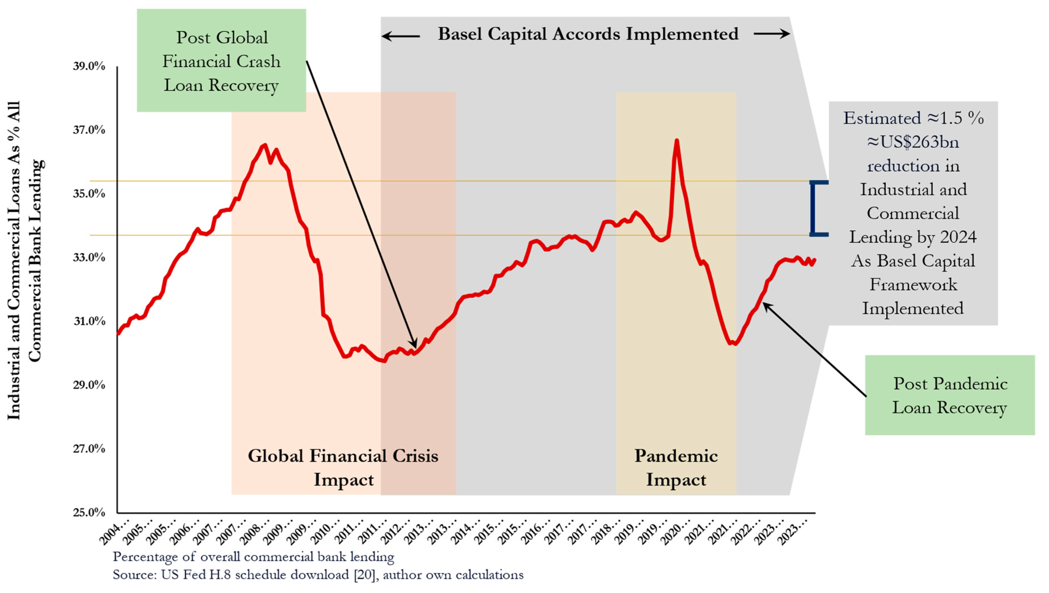
Figure 2.
US Commercial Bank Lending Split 2004. Combined Real and Non-Real Estate Loans = 61.0% of GDP.
Figure 2.
US Commercial Bank Lending Split 2004. Combined Real and Non-Real Estate Loans = 61.0% of GDP.
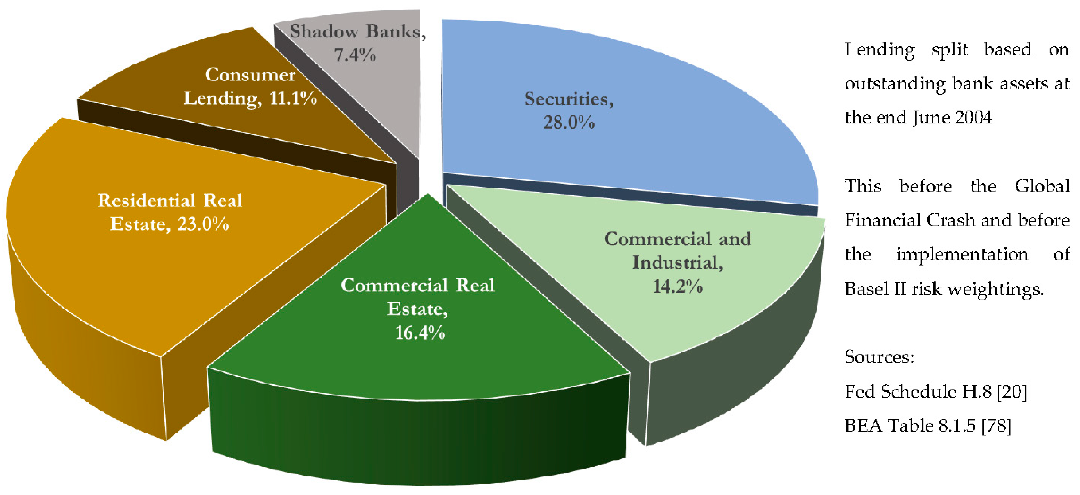
Figure 3.
US Commercial Bank Lending Split 2024. Combined Real and Non Real Estate Loans = 83.3% of GDP.
Figure 3.
US Commercial Bank Lending Split 2024. Combined Real and Non Real Estate Loans = 83.3% of GDP.
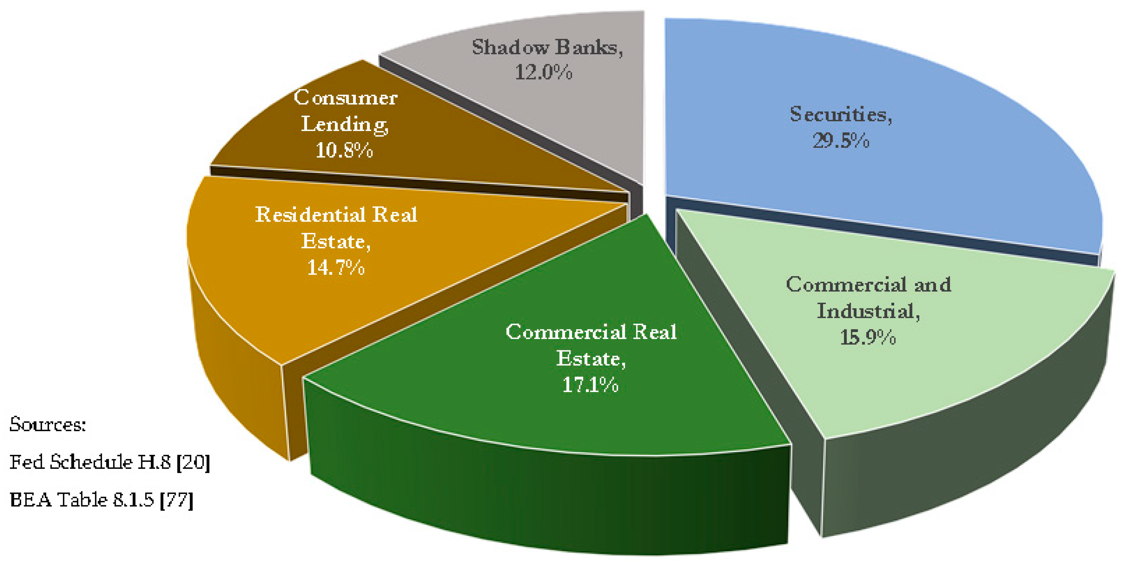
Figure 4.
Change In Loan Demand And Supply Reported By Bank Officers.
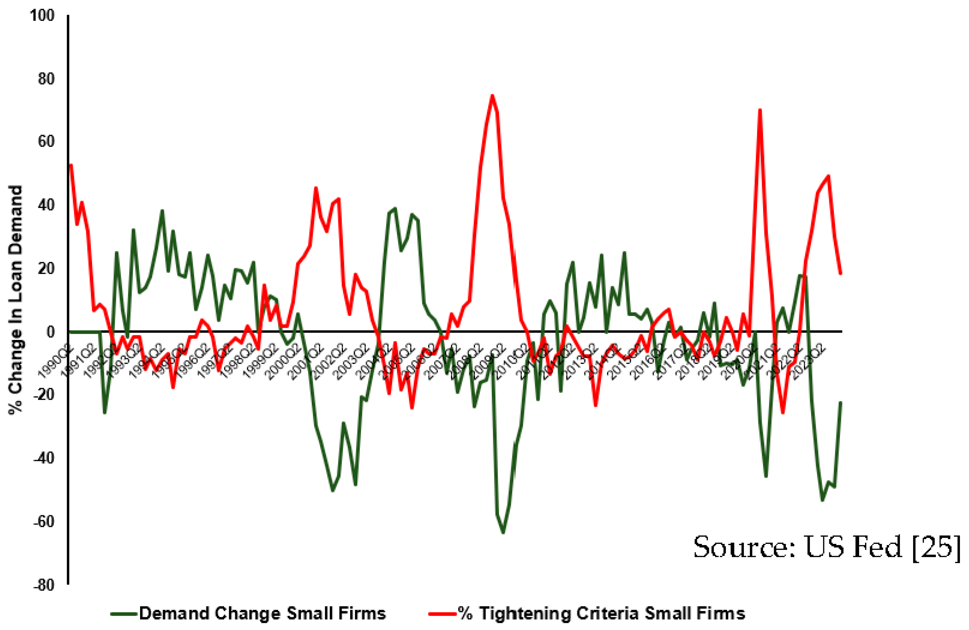
Figure 5.
Drawn Down and Available Credit.
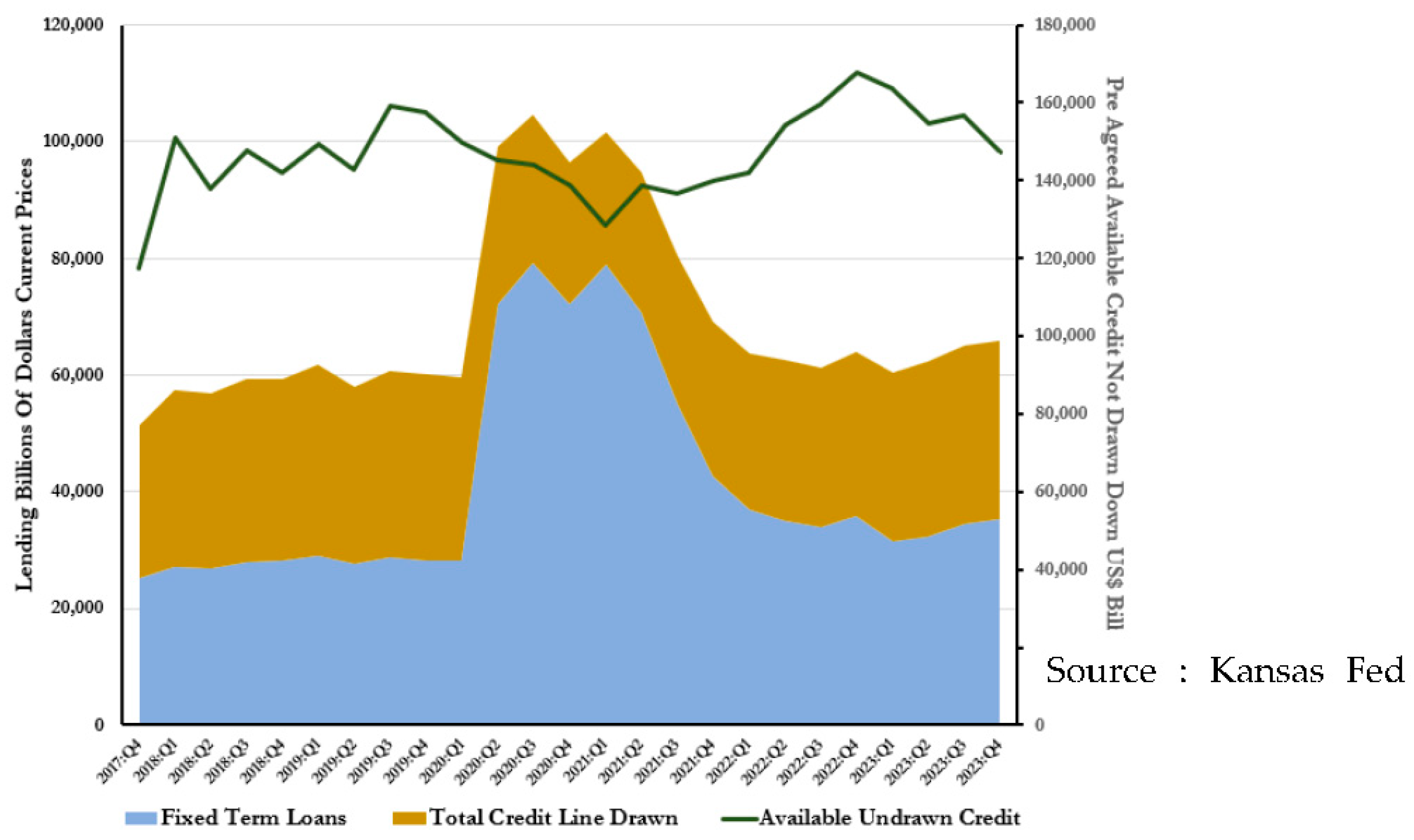
Figure 6.
April 2024 US Commercial Bank Money Transmission Channel.
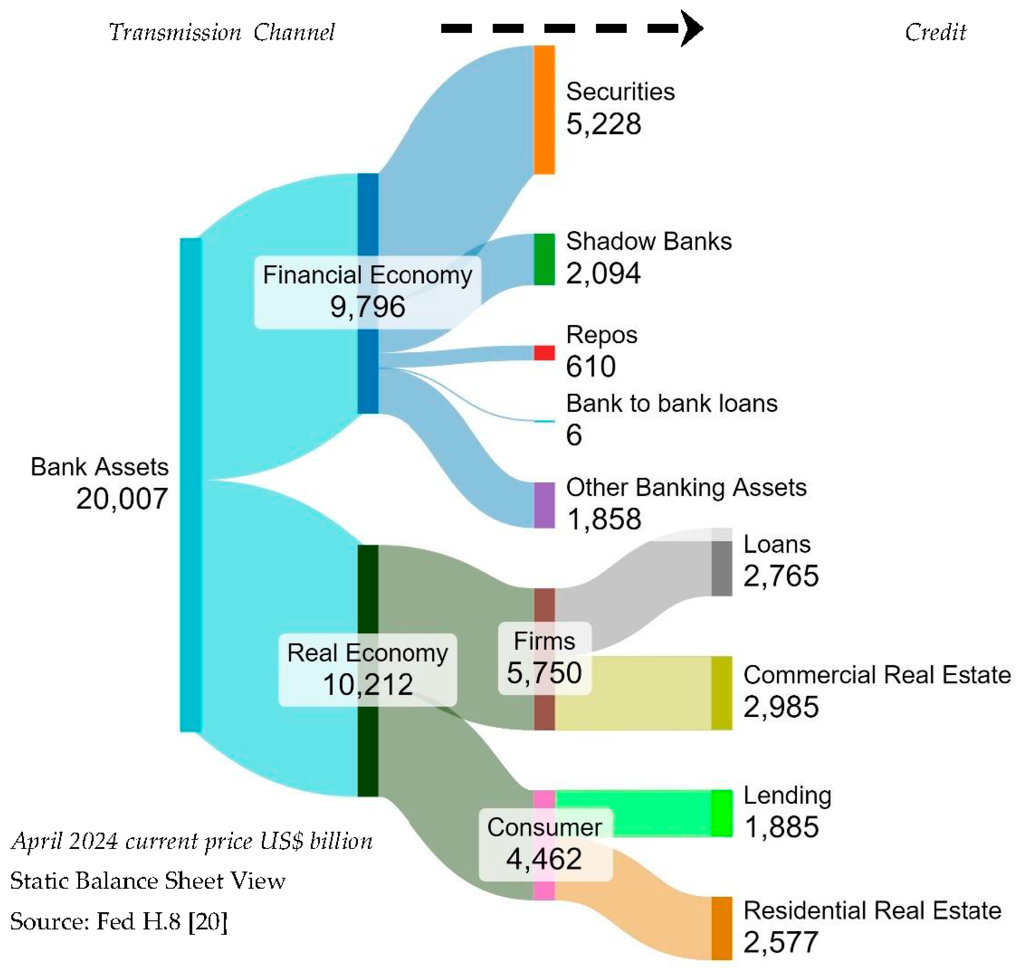
Figure 7.
Contrast Between Large And Small Business Lending.
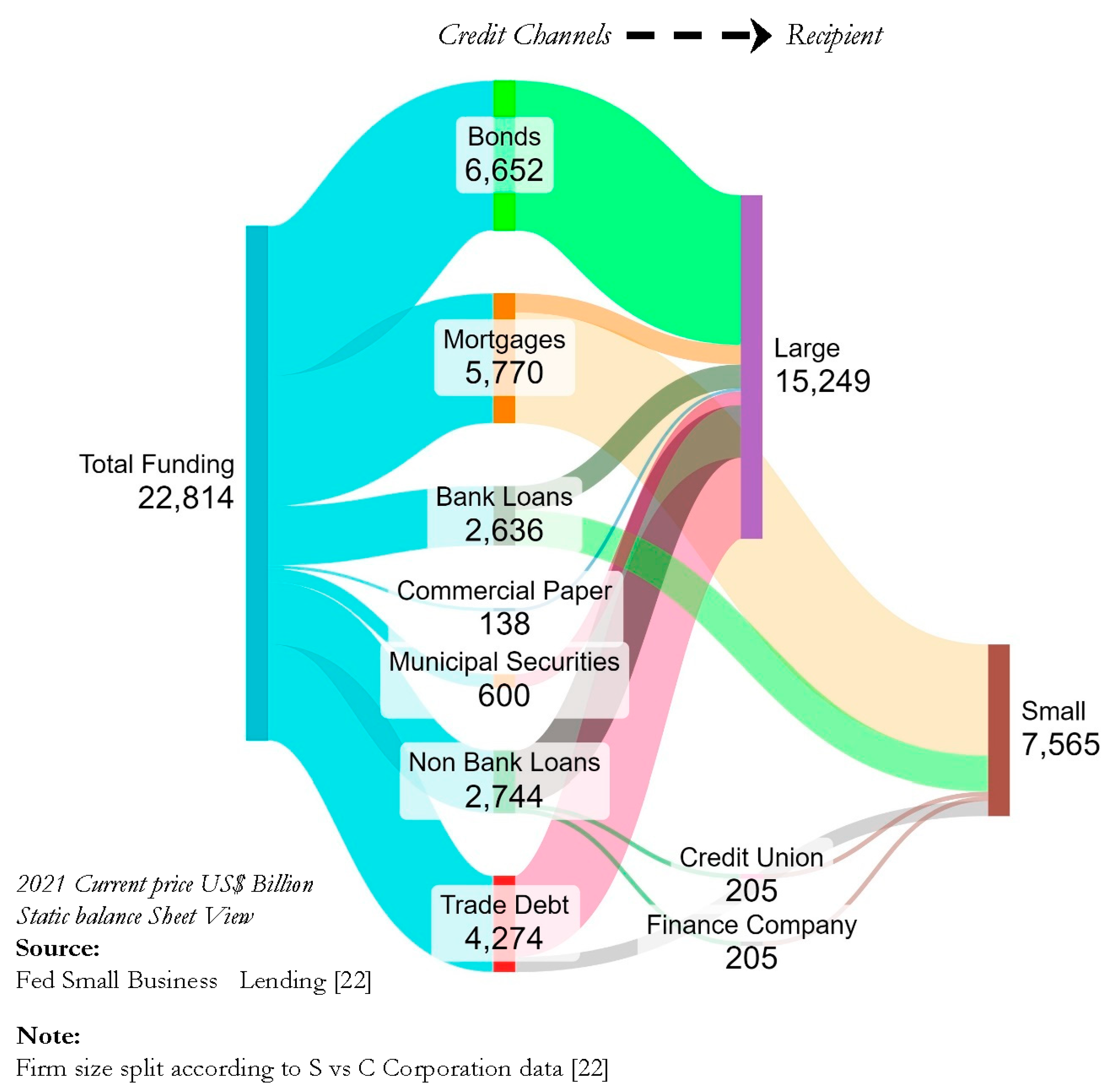
Figure 8.
Community Stable Coin Concept.
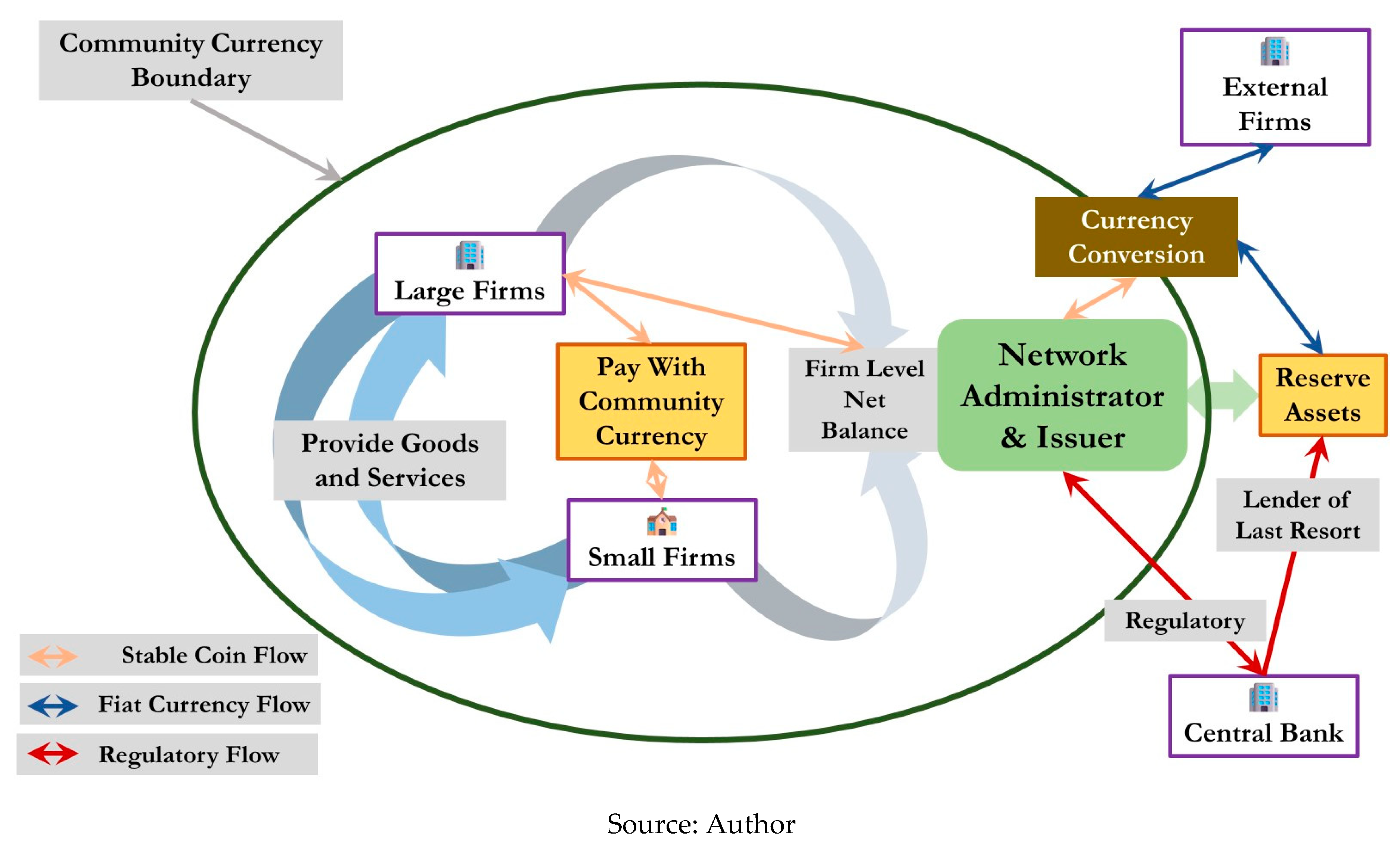
Figure 9.
Stable-Coin Transaction Flow.
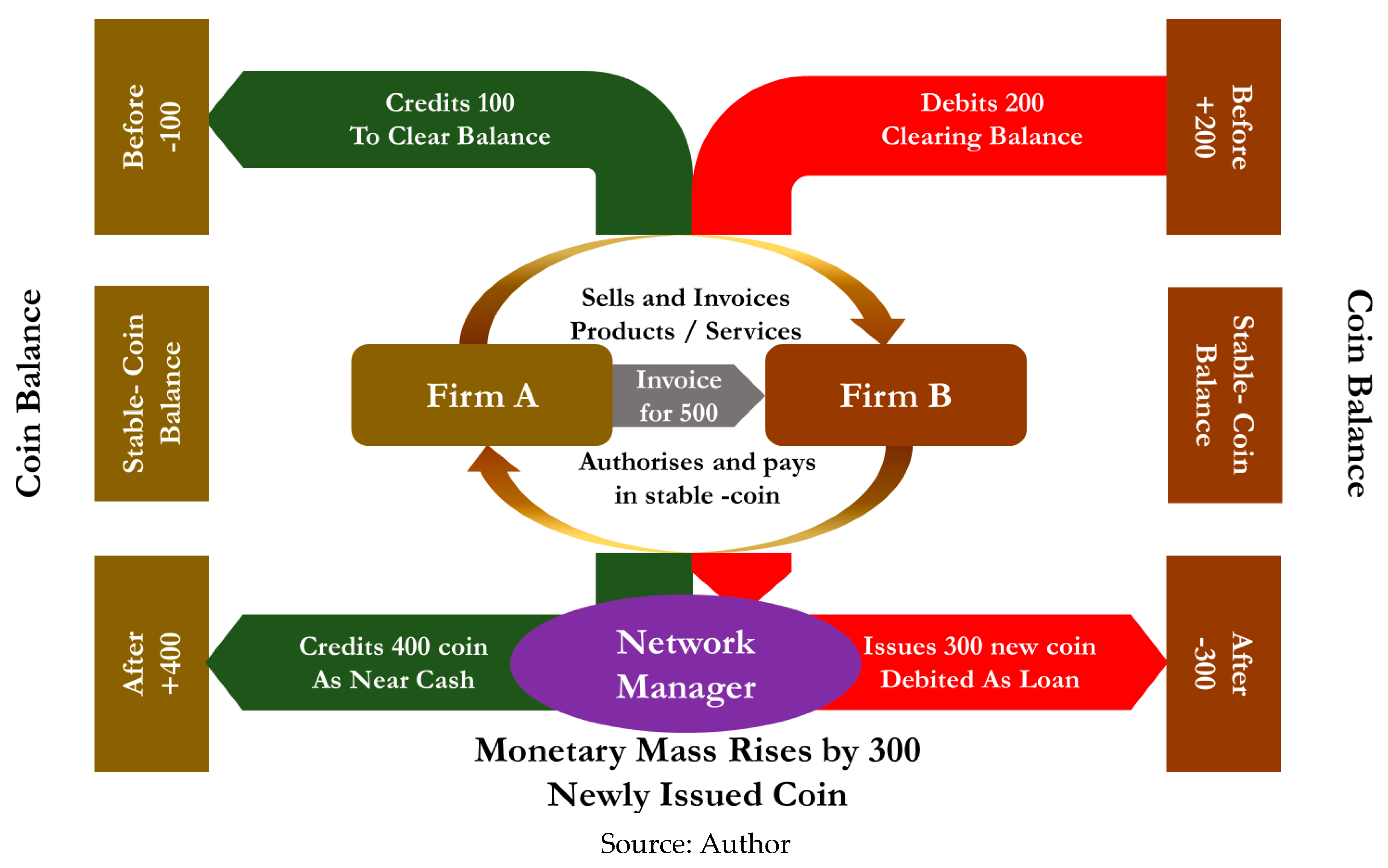
Figure 10.
High Level Fiat Currency Conversion Concept.
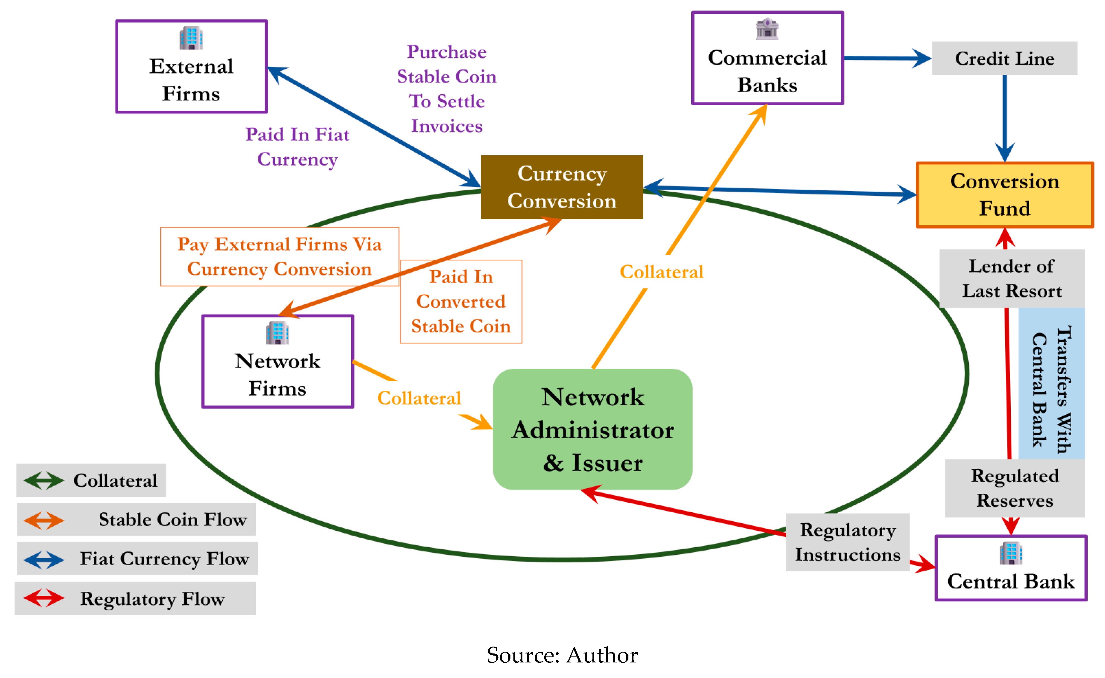
Figure 11.
Stable Coin - Potential US Monetary Mass Impact.
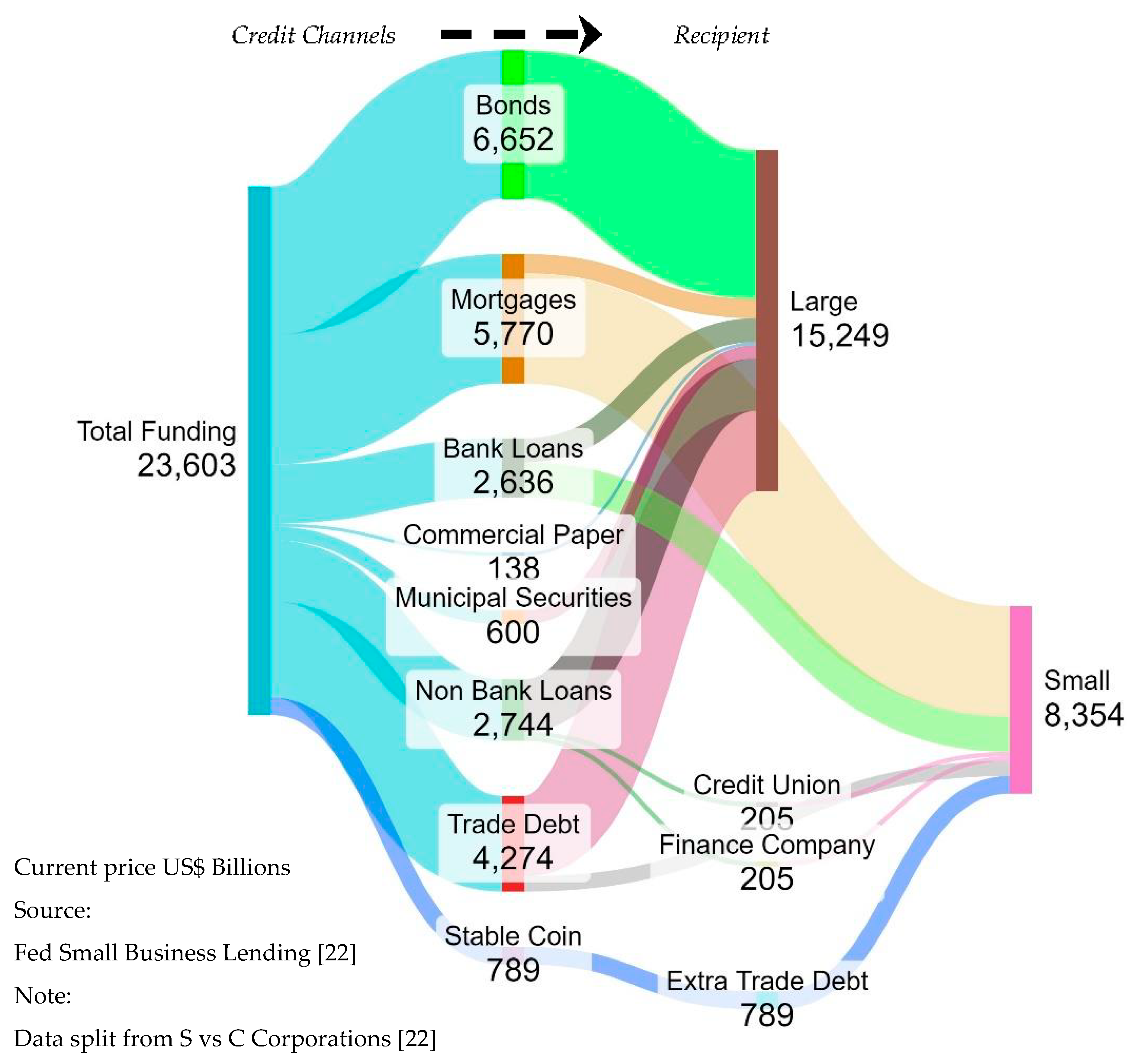

Table 1.
Monetary Transmission Universe.
| Monetary Transmission Space | Credit Channel | Credit Product |
|---|---|---|
| Commercial Banking |
|
|
| Shadow Banking |
|
|
| Crypto - Assets |
|
|
| Central Bank / State |
|
|
| Commercial |
|
|
Table 2.
Small Firm Commercial Bank Lending As Percentage of GDP.
| Year | USA | China | UK |
Sources and Notes: USA: Federal Reserve Financial Access Surveys 2017 & 2022 [23] and [22] China: SME Research Report [67] UK: House of Commons Research [68] China & UK : IMF Financial Access Survey [31] GDP Growth : IMF Financial Access Survey [76] Notes: UK only expresses SME activity as a % of turnover; USA and China are as % GDP US expressed as % 2017 constant price GDP |
|
| 2011 | 24.33 | 31.84 | 11.36 | ||
| 2012 | 24.47 | 35.09 | 10.29 | ||
| 2013 | 24.29 | 35.12 | 9.33 | ||
| 2014 | 24.58 | 36.29 | 8.97 | ||
| 2015 | 25.59 | 36.62 | 8.55 | ||
| 2016 | 26.31 | 36.00 | 8.29 | ||
| 2017 | 27.58 | 36.00 | 7.93 | ||
| 2018 | 29.59 | 35.56 | 7.69 | ||
| 2019 | 31.05 | 37.10 | 7.49 | ||
| 2020 | 33.68 | 41.67 | 10.11 | ||
| 2021 | 28.09 | 41.75 | 9.21 | ||
| Av % Real GDP Growth 2011-21 | |||||
| 2.3% | 7.0% | 1.4% | |||
Table 3.
US Dollar Lending To Non Financial Firms 2011 - 2021.
| 2017 Constant Price | |||||||||||
|---|---|---|---|---|---|---|---|---|---|---|---|
| US$ Billions | 2011 | 2012 | 2013 | 2014 | 2015 | 2016 | 2017 | 2018 | 2019 | 2020 | 2021 |
| Total debt | 6,933 | 7,153 | 7,431 | 7,745 | 8,208 | 8,519 | 8,907 | 9,383 | 9,706 | 10,421 | 10,324 |
| Industrial Revenue & Corporate Bonds | 4,403 | 4,674 | 4,891 | 5,102 | 5,486 | 5,706 | 5,352 | 5,396 | 5,563 | 6,108 | 5,895 |
| Mortgages | 623 | 477 | 452 | 408 | 446 | 479 | 532 | 608 | 650 | 681 | 761 |
| Bank loans not secured on real estate | 684 | 758 | 824 | 884 | 959 | 996 | 893 | 974 | 989 | 1,046 | 946 |
| Commercial paper | 126 | 138 | 152 | 188 | 181 | 185 | 205 | 190 | 187 | 124 | 122 |
| Municipal securities | 0 | 0 | 0 | 0 | 0 | 0 | 570 | 554 | 561 | 555 | 532 |
| Other loans (Shadow Banks) | 1,096 | 1,105 | 1,114 | 1,163 | 2,099 | 1,153 | 1,354 | 1,660 | 1,758 | 1,906 | 2,068 |
| MEMO Trade debt | 1,926 | 1,957 | 2,031 | 2,157 | 2,099 | 2,170 | 2,352 | 2,611 | 2,793 | 2,875 | 3,189 |
| Percentages of GDP | |||||||||||
| 2017 Constant Price | 2011 | 2012 | 2013 | 2014 | 2015 | 2016 | 2017 | 2018 | 2019 | 2020 | 2021 |
| Mortgages | 3.6% | 2.7% | 2.5% | 2.2% | 2.3% | 2.5% | 2.7% | 3.0% | 3.1% | 3.2% | 3.5% |
| Bank loans not secured on real estate | 3.9% | 4.3% | 4.6% | 4.7% | 5.0% | 5.1% | 4.5% | 4.8% | 4.8% | 5.0% | 4.3% |
| Industrial Revenue & Corporate Bonds | 25.4% | 26.5% | 27.2% | 27.3% | 28.9% | 29.4% | 26.7% | 26.4% | 26.9% | 29.1% | 27.1% |
| Commercial paper | 0.7% | 0.8% | 0.8% | 1.0% | 1.0% | 1.0% | 1.0% | 0.9% | 0.9% | 0.6% | 0.6% |
| Municipal securities | 0.0% | 0.0% | 0.0% | 0.0% | 0.0% | 0.0% | 2.8% | 2.7% | 2.7% | 2.6% | 2.4% |
| Other loans (Shadow Banks) | 6.3% | 6.3% | 6.2% | 6.2% | 11.0% | 5.9% | 6.8% | 8.1% | 8.5% | 9.1% | 9.5% |
| Trade Debt | 11.1% | 11.1% | 11.3% | 11.6% | 11.0% | 11.2% | 11.7% | 12.8% | 13.5% | 13.7% | 14.7% |
Table 4.
US Dollar Lending To Small US Firms 2011 - 2021.
| 2017 Constant Price | |||||||||||
| Billions US$ | 2011 | 2012 | 2013 | 2014 | 2015 | 2016 | 2017 | 2018 | 2019 | 2020 | 2021 |
| Total debt | 4,226 | 4,321 | 4,361 | 4,589 | 4,862 | 5,104 | 5,528 | 5,692 | 5,870 | 6,260 | 6,106 |
| Mortgages | 3,059 | 3,098 | 3,128 | 3,274 | 3,451 | 3,635 | 3,915 | 4,029 | 4,208 | 4,372 | 4,352 |
| Bank loans (not real estate secured) | 980 | 1,031 | 1,037 | 1,112 | 1,204 | 1,261 | 1,376 | 1,422 | 1,417 | 1,557 | 1,390 |
| Shadow Bank loans (not real estate secured) | 186 | 193 | 196 | 202 | 207 | 207 | 237 | 241 | 245 | 331 | 363 |
| MEMO Trade debt | 525 | 526 | 553 | 555 | 603 | 653 | 588 | 581 | 614 | 579 | 598 |
| Percent SME 2017 Constant Price GDP | |||||||||||
| Mortgages | 40% | 40% | 40% | 40% | 42% | 43% | 45% | 45% | 47% | 48% | 46% |
| Credit Union Supplied | 1.2% | 1.3% | 1.3% | 1.2% | 1.3% | 1.2% | 1.4% | 1.4% | 1.4% | 1.8% | 1.9% |
| Finance Company Supplied | 1.2% | 1.3% | 1.3% | 1.2% | 1.3% | 1.2% | 1.4% | 1.4% | 1.4% | 1.8% | 1.9% |
| Trade Debt | 7.0% | 6.8% | 7.1% | 6.8% | 7.3% | 7.7% | 6.7% | 6.5% | 6.8% | 6.3% | 6.3% |
| Total | 55.9% | 56.2% | 55.8% | 56.5% | 58.8% | 60.5% | 63.4% | 64.1% | 65.3% | 68.6% | 64.6% |
Sources: Fed Reserve Financial Access Surveys 2017 & 2022 [22,23] and [19]. Footnote 5 page 7 [22] implies data for S Corporations. Note: S Corporations are used small businesses proprietorships and partnerships, C Corporations are for larger firms. Referenced footnote is unclear, data results make clear that two different data collection sources were used. Nonfinancial entity assignment comes from the designated entity Standard Industrial Classification held in firm’s legal registration.
Table 5.
Major Differences in Funding Sources Between Small Firms and Industrial and Commercial Firms.
Table 5.
Major Differences in Funding Sources Between Small Firms and Industrial and Commercial Firms.
| 2017 Constant Price GDP | 2011 | 2012 | 2013 | 2014 | 2015 | 2016 | 2017 | 2018 | 2019 | 2020 | 2021 |
|---|---|---|---|---|---|---|---|---|---|---|---|
| Mortgages as % GDP | |||||||||||
| Small | 40.5% | 40.3% | 40.1% | 40.3% | 41.8% | 43.1% | 44.9% | 45.4% | 46.8% | 47.9% | 46.0% |
| All | 3.6% | 2.7% | 2.5% | 2.2% | 2.3% | 2.5% | 2.7% | 3.0% | 3.1% | 3.2% | 3.5% |
| Non Real Estate Loans % GDP | |||||||||||
| Small | 13.0% | 13.4% | 13.3% | 13.7% | 14.6% | 14.9% | 15.8% | 16.0% | 15.8% | 17.1% | 14.7% |
| All | 3.9% | 4.3% | 4.6% | 4.7% | 5.0% | 5.1% | 4.5% | 4.8% | 4.8% | 5.0% | 4.3% |
| Bonds As % GDP | |||||||||||
| Small | 0.0% | 0.0% | 0.0% | 0.0% | 0.0% | 0.0% | 0.0% | 0.0% | 0.0% | 0.0% | 0.0% |
| All | 25.4% | 26.5% | 27.2% | 27.3% | 28.9% | 29.4% | 26.7% | 26.4% | 26.9% | 29.1% | 27.1% |
| Trade Debt (Memo estimate) | |||||||||||
| Small | 7.0% | 6.8% | 7.1% | 6.8% | 7.3% | 7.7% | 6.7% | 6.5% | 6.8% | 6.3% | 6.3% |
| All | 11.1% | 11.1% | 11.3% | 11.6% | 11.0% | 11.2% | 11.7% | 12.8% | 13.5% | 13.7% | 14.7% |
Table 6.
Calculated US Small Firm Working Capital Requirements.
| Trade Debt | 2011 | 2012 | 2013 | 2014 | 2015 | 2016 | 2017 | 2018 | 2019 | 2020 | 2021 |
|---|---|---|---|---|---|---|---|---|---|---|---|
| Small Firms% SME GDP | 7.0% | 6.8% | 7.1% | 6.8% | 7.3% | 7.7% | 6.7% | 6.5% | 6.8% | 6.3% | 6.3% |
| Large Firms % all GDP | 11.1% | 11.1% | 11.3% | 11.6% | 11.0% | 11.2% | 11.7% | 12.8% | 13.5% | 13.7% | 14.7% |
| Difference | 4.1% | 4.2% | 4.2% | 4.7% | 3.8% | 3.4% | 5.0% | 6.2% | 6.7% | 7.4% | 8.3% |
| SME Current Price GDP | 6,728 | 7,008 | 7,259 | 7,581 | 7,901 | 8,109 | 8,428 | 8,890 | 9,255 | 9,262 | 9,977 |
| Unconstrained SME trade debt (calc from SME GDP) | 746 | 776 | 821 | 876 | 873 | 907 | 989 | 1,137 | 1,251 | 1,268 | 1,464 |
| Actual SME Trade Debt | 483 | 494 | 528 | 537 | 588 | 646 | 593 | 599 | 642 | 615 | 675 |
| Gap (Est. Additional Funding Requirement) | 263 | 282 | 293 | 339 | 285 | 261 | 396 | 538 | 609 | 653 | 789 |
Disclaimer/Publisher’s Note: The statements, opinions and data contained in all publications are solely those of the individual author(s) and contributor(s) and not of MDPI and/or the editor(s). MDPI and/or the editor(s) disclaim responsibility for any injury to people or property resulting from any ideas, methods, instructions or products referred to in the content. |
© 2024 by the authors. Licensee MDPI, Basel, Switzerland. This article is an open access article distributed under the terms and conditions of the Creative Commons Attribution (CC BY) license (http://creativecommons.org/licenses/by/4.0/).
Copyright: This open access article is published under a Creative Commons CC BY 4.0 license, which permit the free download, distribution, and reuse, provided that the author and preprint are cited in any reuse.


