Submitted:
25 May 2024
Posted:
27 May 2024
You are already at the latest version
Abstract
The increasing prevalence of species that are detrimental to biodiversity is a major concern, particularly for managers of National Parks. To develop effective programs for controlling weeds, it is essential to have a thorough understanding of the extent and severity of infestations, as well as the contributing factors such as temperature, rainfall, and disturbance. Predicting these factors on a regional scale requires models that can incorporate a wide range of variables in a quantifiable manner, while also assisting with on-ground operations. In this study, we present two Bayesian Network models specifically designed for six significant weed species found along the southern coast of Australia. Our models are based on empirical data collected during a coastal weed survey conducted in 2015 and repeated in 2016. We applied these models to the coastal national parks in the isolated and pristine East Gippsland region. Importantly, the prediction models were developed at two different spatial scales that directly corresponded to the scale of the observations. Our findings indicate that coastal habitats, with their vulnerable environments and prevalence of open dune systems, are particularly susceptible to weed infestations. Moreover, adjacent regions also have the potential for colonization if these infestations are not effectively controlled. Climate-related factors play a role in moderating the potential for colonization, which is a significant concern for weed control efforts in the context of global climate change.
Keywords:
Weeds
; Bayesian Networks
; biodiversity management
; coastal systems
1. Introduction
The management of biodiversity within conservation reserves requires the control of species that expand their range at the detriment of other species. In regions that are relatively pristine in terms of disturbance, this change is inherently obvious as so called ‘weeds’ colonize available space rapidly [1]. Often this process is assisted by the disturbance generated by external factors such as fires, animals and humans. Direct control of the weeds becomes a priority before the system is beyond repair and the ecosystems are required to accept the change to a novel ecosystem [2].
Early intervention is difficult when the vast area of the conservation area is inaccessible except by foot and weed control requires significant physical and chemical effort to have any noticeable effect [3]. This translates directly to high yearly expenditure on weed control and detection with significant demands to spatially prioritize efforts [4]. The development of a strategic plan to ensure the greatest effectiveness of control efforts is essential but these plans are often constructed in the face of high data uncertainty and inadequate weed behaviour models. On-ground surveys need to be fully leveraged to expand and interpolate weed presence/absence observations to regions that were unable to be surveyed. Supporting data, such as the spatial extent of vulnerable vegetation communities, is required to provide a regional assessment. However combining all these qualitative and quantitative datasets with the purpose of estimating the presence or not of a particular weed species or pest is not trivial [3,5].
Utilising the theories of ecological niche and environmental gradients is the foundation of habitat suitability probability modelling [6,7]. In this framework the observation of the presence of weeds is statistically correlated to a suite of environmental conditions. For many applications of this approach the assumption is that the system is in equilibrium and the absence of a species at an observed location indicates the likelihood of unsuitable environmental conditions [7]. However, for emerging weeds that are in the early stages of colonization, the observation of ‘species absent’ has an additional meaning that the survey space may simply have avoided colonization due mainly to stochastic events. This habitat suitability dynamic is also complicated when survey results are incomplete due to resource limitations. The statistical correlations then will be ‘weak’ for weed species that may only occur in small fractions of the available habitat. It may even be possible that suitable habitat is incorrectly classified as ‘unsuitable’ because the correlation has not been observed. Increased sampling effort combined with systematic sampling design will assist [6] but expert opinion on specific weed species preferences may also be required. This expertise can often be acquired from weed occurrences in adjunct regions.
With such uncertainty regarding the impact and colonization success of weeds in a conservation area the use of an adaptive management framework is important [8]. Routine field work such as track maintenance and visitor facility upkeep can be combined with biodiversity actions such as weed control and survey [9]. Ideally the feedback mechanisms in place for conservation managers, from weed observations to modelled vulnerability, can assist with a dynamic prioritization of targeted control actions. Equipping land managers with both the tools and knowledge to capture weed observations and environmental conditions is optimal to modelling the extent of the issues in the region [6]. Habitat suitability modelling will require a sophisticated capacity to integrate disparate data and provide rapid updates of the infestation extent and intensity including previous measures of success in infestation control and contributing factors (i.e. soil disturbance). Adaptive management of the conservation areas require a close linkage between monitoring, objectives and action [10]. Critically conservation managers require a model of the vulnerability of weed infestations across a range of habitat types (to assist in survey strategies) combined with another model of site-level contributing factors that can be physically controlled.
Models suitable for this environment management need to be able to combine disparate data and require a common ‘currency’ to determine the relationships within the model. Simply combining presence/absence of a weed with the coincident observation of a suite of environmental parameters ignores the complexities of the multicollinearity relationships between dependent variables [11], i.e. rainfall, soil type and disturbance. In order to restrain the model complexity to maintain predictive power while negotiating uncertainty limits and yet offer spatially valid estimations of vegetation dynamics will require alternative modeling approaches [12]. One such approach is to base the probabilistic predictions on correlations between observations over space and time rather than formulate a set of precise interaction equations [13]. Correlations in a trophodynamic system do not necessarily directly equate to metabolic, behavioral or ecological processes but the tradeoff is the ability to predict with increased precision in a diverse and uncertain environment [14].
Bayesian Networks (BN) are one such modelling technique that is particularly popular in ecology due to the capacity to support both complexity and uncertainty simultaneously [15,16]. BN offer the capacity to encompass complex interactions of disparate data types within a probabilistic framework with only a few limitations [17,18,19,20]. Bayes rule, combined with the chain rule, enable the efficient propagation of conditional probability throughout a network structure [21,22]. The network design is typically the result of expert opinion although machine learning algorithms exist to formulate a possible network structure through analysis of correlations [20]. The parameterization of a BN model is through the inclusion of observational cases that fully or partly describe a system state. The more cases used to inform the conditional probabilities, within the model, the more accurate the predictions [13]. Algorithms, such as expectation maximization, can assist in adjusting for missing data [23]. Expert opinion, equations, numerical (continuous, discrete and censored) data and categorical data can be included in the model, which is particularly useful for socioecological models [15].
Limitations relevant to ecosystem models include the prohibition of feedback loops and the inability to predict outside of the observational space [16]. Feedback loops, in particular, have severely limited the application of BN to trophic dynamics but recent advances in network analysis [18] and time aggregation have established an acceptable compromise. Eklöf et al. [18] demonstrated the application of BN to extinction rates in food web models via the simplification and retention of fundemental pathways between groups of species. The BN is able to predict the likelihood of a system being in a particular state given additional evidence. However, this requires that the conditional probabilities (from observed cases) have been previously included in the model parameters. Predicting how the system will respond to conditions outside of the observation space require the inclusion of expert-derived predictions, often in the form of equations, generated from models such as IPCC climate models or experiments on metabolic thresholds. Even with such input the propagation of predictions to unobserved biotic interactions becomes uncertain with a significant loss of accuracy.
Interestingly, the primary concepts behind BNs are familiar to the general population. For example, when assessing the appropriate clothes to wear for a walk in the forest people will gather up information about the likely weather patterns, the seasonal influences, the past experiences (being too hot or cold), and the available selection of clothes. The walker has a priori knowledge that the weather is uncertain and that events have a range of probabilities depending on the season and daily factors. The estimation of these probabilities in our minds is a regular occurrence but few people would use a mathematical approach to carefully define the likelihoods. The Bayes theorem permits the calculation of these probabilities so that we are not solely reliant on expert opinion and vulnerable to surprises [23].
Here we present the results of the two BN models that incorporates a range of influential data sets to generate predictive maps of weed distributions. Complimentary BN models at two alternative spatial scales are presented as a mechanism to assist with the adaptive management of an expansive conservation area. The two models presented are, in themselves, interesting reflections of the influences that determine the weed dynamics. The questions we address have a different focus. What ecosystems are vulnerable to weed infestations across the entire East Gippsland national park (in Victoria, Australia)? What contributing factors can be managed at the site level to control weed infestations?
2. Materials and Methods
In brief the methods consisted of four parts: The collection of weed observations and in situ environmental data across the study area, the compilation of geospatial data for use in a regional scale model, the development of a casual network to inform the Bayesian network.
2.1. The East Gippsland Study Area
The spectacular and unspoilt coastline of the East Gippsland study area includes UNESCO World Biosphere Reserves amongst a diverse suite of inlets, rocky headlands and isolated beaches (Figure 1). The enormous diversity of ecosystems from heathlands, dunes, rainforests and majestic forests attracts visitors both nationally and internationally. The study area includes Croajingolong NP, Cape Conran NP, Peach tree Creek Reserve. The study area is 100,094 Hectares with 176 km length of coastline with no significant human habitation in the region.
2.2. The Weeds Survey
Within the study area the following landforms and features were surveyed for weeds:
- Beach Strand. The area of beach between the high tide line and dunes.
- Dune complex. Primary (first) dune and swale beyond above beach strand.
- Rocky Headlands. Elevated cape or point of land reaching out into the water, devoid of beach strand or dune characteristics.
- Estuarine Shores. Areas of land abutting estuarine waters at the time of survey to a maximum of 250 metres inland.
- Human Access Nodes. Areas readily and frequently accessed by recreational users comprising: the last 100m of vehicular tracks servicing carparks and lookouts, 20m buffer around lookouts, carparks and campgrounds.
Three key survey methods were applied across the study area:
- 6.
- Random stratified sampling (unbiased) of transects. Generation of 90 random point locations (using ET Geowizard within ARCGIS 10) within the Ecological Vegetation Class (EVC) layer based on each area of an ecological vegetation class.
- 7.
- Random sampling (biased) of past infestations. Biased random transects across 110 locations within areas where weed species have previously been recorded.
- 8.
- Opportunistic searching. Data on weed species was recorded throughout the entire study area through meander searching. This involved crews of two people walking the entire stretch of the coastline within the study area between Point Ricardo and the NSW border.
For the surveys along the Dune complex the 3-way transect method was used. This required the surveyors to start at the beach then head inland up to 100m inland (perpendicular to the water’s edge) over the fore dune and into the swale (where practical). Then the surveyors follow for 100m along the swale or dune. Finally, the surveyors turn back out to the beach recording along all three sections. The weed cover and extent was recorded by the two surveyors who walked either side of the center of the transect line (covering an estimated survey width of 20m along each transect). A GPS was used to record the start and end points of each transect line (including change of direction) and location of weed species and related attributes (Table 1). Additional site based observations were also collected (Table 2).
For the estuary or campground and activity nodes, the transect location involved the completion of a 2-way transect. The transect was commenced at the estuary or campground activity-node edge, heading directly away approximate center of the node for 20m.
The weed surveys conducted in November 2015 and 2016 noted 6 key species that were significant invasive pests in the region [9]. 2522 survey sites (1486 in 2015 and 1036 in 2016) were recorded along the coastline and the presence and absence of key weed species noted as well as a range of environmental conditions. The primary weed species of concern were Coastal Gladiolus (Gladiolus gueinzii), Coastal Capeweed (Arctotheca calendula), Dolichos Pea (Dipogon lignosus), Purple Groundsel (Senecio elegans), Tree Lupin (Lupinus arboreus) and Sea Spurge (Euphorbia paralias). Other weeds were also identified but not included in this predictive model to constrain the complexity of the outputs. Sites with no visible signs of weed presence were also noted.
2.3. Model Development
The primary motive for this project was to develop a regional model of the vulnerability of key weed species for the entire study area. However given the imperative to address adaptive management processes, a local site scale model was also developed directly from the environmental and weed observation data. While the regional scale model utilized covariate data that was recorded or modelled across the region to develop a spatially explicit set of predictions, the local site model was not spatially explicit and captured fine scale observations that were pertinent to field-based operatives.
2.4. Regional Scale Weed Vulnerability BN
The critical first step to the regional model development is the construction of a causal diagram [24] for the immergence of weeds across the region. This required many iterations based on expert opinion to successfully capture the environmental influences and their association to weed colonization. Many region-scale environmental variables could have been included but were excluded simply due to the constraint of keeping a model sufficiently simple and manageable. Complementing this process was the availability of data that was sufficiently high resolution, temporally relevant and had regional coverage. Spatial information on the activities of feral animals, for example, was not available with sufficient accuracy to include. Finally, the network diagram showing the various parameters and the cross linkages was agreed on by the authors. The site scale model, in contrast, used a machine learning tree-augmented naïve (TAN) algorithm based on the survey data alone to generate a BN model [25].
Data collection of environmental variables at the scales of the model output were gathered or created using GIS modelling techniques. The various data sources and complimentary metadata are listed in Table 3. GIS analysis was conducted in QGis Version 2.18.2 (QGIS Development Team, 2009). The resolution of the output was determined at 30 metres by 30 metres in order to capture some fine scale features (precision) but remain sufficiently robust (accuracy) for the regional approach.
For every weed species, the spatial points showing the observed occurrence and the observations without any weeds were placed in separate shapefiles. The values for the raster environmental and GIS model data was extracted to every survey point. The attributes were exported, examined and consolidated in R (Version 3.3.2)( R Core Team 2017). The scripts in R created a text file (referred to here as a ‘case’ file) where every spatial point was a data frame row with column information pertaining to the various list of model parameters. Three case files were created for each weed. The first was the full survey case file with the associated environmental data. The second and third case files were the same file but randomly sampled for 20% and complimentary 80% of the data.
The causal network formed the basis of a naive Bayesian Network (BN) within the Netica V6.04 software environment (Norsys Software Corp 2016). The conditional probability tables (CPT) were updated by importing the 80% survey case file for the single weed using an expectation maximization procedure. This algorithm is particularly suited to data that contains significant levels of missing data [23]. The BN model was compiled and contained the marginal probabilities for each parameter. Essentially this was a reflection of the observed likelihood of any parameter occurring in the survey data set, similar to a histogram but with bins sizes reflecting the frequency of data.
The BN was then tested for predictive accuracy for each weed species using the associated 20% reduced dataset. The testing compared the observations of species occurrence with the BN predictions given the environmental data. This generated a number of indices (Correlation matrix error, Gini Coefficient and Area under ROC) that provide a measure of accuracy of the model structure and parameterization [26]. The full survey case file was then used to totally update the CPT probabilities.
The study region case file was compiled from the centroids of all 30m x 30m raster cells in the study polygon and attributed with the regional datasets listed in Table 3. This was used to predict the likelihood of a selected weed occurring within the entire study area. A new file that recorded the probability of a particular weed occurring, given the conditional probability of the environmental and social parameters, was generated. This file was subsequently joined to the spatial points file and used to map the distributions in the GIS.
The process of CPT updating is repeated for every key weed species so that the BN model structure (based on the causal diagram) remains consistent but the marginal probabilities are adjusted accordingly.
2.5. Local Site Scale BN
A second model was also developed from the information contained in the survey data alone. This model was not spatially explicit due to the fine scale nature of the field based observations and was used to describe the mechanisms that determine the local scale processes promoting the occurrence and spread of the weeds. The selection of parameters to collect was based on the expert opinion of field staff with particular focus on Victorian National Parks operational management. The TAN machine learning algorithm used the structure of the field survey data associations to develop the BN with the ‘common weed names’ as the target variable. The survey parameters observed during the field trip are detailed in Table 1 and Table 2. This model, due to the key factors observable only at a site level (i.e. soil disturbance and drainage), cannot be extrapolated to a regional scale but still serves to provide insights into the influences affecting weed spread. Critically, this model can inform park managers about the actions required to control weed infestations at a site level. This approach of generating two models at different scales supports the adaptive management framework by providing synthesized information about weed behaviour. Following systematic repeated surveys the data can also reveal the effectiveness of control measures, vulnerability of habit types and influential socioecological factors in weed colonization.
3. Results
A linear distance of approximately 176km of coast was surveyed in 2015 and repeated in 2016. During the 2016 survey, 173 transects were completed and 27 transects were abandoned and not completed due to steep inaccessible terrain, very close proximity of a transect to another transect or lack of time on the day surveying to complete the transect. The combined linear distance of transects is 2.3km. A total of 84 different weed species (of which 8 were on adjoining private land) and 1,538 weed records were captured during the survey. The 10 most frequent weed species recorded during the survey were Milk Thistle (Sonchus sp., 33), Flatweed (Hypochaeris sp. 35), Blackberry (Rubus fruticosus aggregate 38), Panic Veldgrass (Ehrharta erecta 47), Dolichos Pea (Dipogon lignosus 50), Sea Rocket (Cakile sp. 76), Coast Gladiolus (Gladiolus gueinzii 87), Marram Grass (Ammophila arenaria 175), Coast Capeweed (Arctotheca populifolia 209) and Sea Spurge (Euphorbia paralias 521). Sea Rocket and Marram Grass are actually the most common and so the number of observations represents the intersects within the transects.
Utilising the survey data combined with the geospatial data two BN models were developed. The site observations were used to construct a BN that provided management orientated outputs useful for on ground operations. The regional vulnerability BN model was able to predict the occurrence of several different weeds along the East Gippsland coastal national parks with mixed accuracy to facilitate weed control priorities.
3.1. Local Site BN
The model configuration is shown in Figure 2 and describes the observations in a 30 metre radius. The error rate of this model was 20.97% based on a confusion matrix with 20% random subset of the survey data (Table 4). Essentially this compared the number of cases allocated by predictions against the observed. For example, in Table 4 138 cases are accurately predicted to be Sea Spurge while in the cell below 11 cases were predicted to be Sea spurge but were actually Coast Capeweed. The marginal probabilities in the local BN model (Figure 2) shows that surveys along the coast were conducted in mostly well drained sandy soils with grassland cover or a dune/scrub/grassland mosaic (Vegetation type node in Figure 2). The observed weeds were predominantly noted as emerging and scattered, often covering a 10 metre square area.
The model can be used to predict the likelihood of weed occurrence if those identified parameters can be estimated. The model calculates the influences present in the model (calculated as variance reduction) as shown in Table 5. Vegetation type (grasslands etc.), behavior (emerging etc.) and soil disturbance (wind etc.) are the most influential nodes. The node ‘Common Name’ shows the occurrence of the observations for the field survey. Sea Spurge rated the most common with 50.3 % of observations while Purple Groundsel was only 0.29%. The absence of weeds was noted in 15.0% of observations and this was used to highlight the more resilient vegetation types.
From a management perspective, the capacity of the model to highlight the most likely site-specific factors that influence the presence of a specific weed is critical. By selecting the common weed name, the model, within Netica software, will automatically adjust the marginal probabilities and present a series of primary factors to observe or control. Given the large area of landscape to manage this capacity to focus on the most likely areas of emerging weeds is highly effective.
3.2. Regional Vulnerability BN Model
The regional vulnerability BN model was built from several iterations of a causal diagram containing nine environmental factors and two social factors (Table 3) .
This BN model is shown in Figure 3. There are 3 main components; Dispersal influences, habitat vulnerability and climate. Each of the nodes (shown as boxes linked in a network) are described in Table 1. Spatial data, where available, was used to populate the model except in three variables called latent nodes. These nodes do not have a spatial dataset and are used to assist with the flow of conditional probability logic through the model and include the Climate, Dispersal influences and Habitat vulnerability nodes. Climate is defined as a mix of geomorphology such as aspect and regional changes in temperature and rainfall. Dispersal influence captures the assisted transport of seeds and plants through vectors such as water and human disturbance. Habitat vulnerability is the combination of geology and existing vegetation types that might hinder or assist the establishment of these weeds [27]. The expectation maximization algorithm is used to ‘shape’ these latent node probabilities beyond simple expert opinion. The probabilities shown in the model in Figure 3 describe the 2522 survey observations and associated environmental data that was used to inform the CPTs customized for each weed species (noting that Figure 3 was the Coastal Capeweed BN). The dominance of coastal scrub along the coastal dunes is evident (Ecological Vegetation Communities node values in Figure 3) and the wilderness of the region is captured by the majority of survey points being away from roads (road cost distance node; mean=964m). The study area is generally dry with 70% of points being more than 170 metres from a creek or water source. The error for the spatially enabled regional BNs for the mix of weeds was estimated at 3.9% to 6.1% based on a confusion matrix in Table 4. The model accuracy was not able to be tested with Purple Groundsel and Tree Lupin due to the small number of observations that denied a sub setting algorithm. Coastal Capeweed, Coastal Gladiolus, Dolichos Pea and Sea Spurge predicted well for the immediate area around the survey sites and the model can be utilized for these species. The Gini coefficient and Area Under Curve (AUC) [26] highlight that for the survey locations the predictions are considered accurate (values close to 1 in Table 6) in being able to predict the existence of the weed species.
The sensitivity of the “Species Occurrence” node to changes in the other nodes was examined for each weed species and shown in Table 7. This table shows that Climate and Dispersal influences (particularly the distance to existing weed populations) are highly influential. Other factors such as distance from a campground were surprisingly weak in influencing the presence of weeds at a regional scale. Notably each weed responds differently to the environmental and social factors (see A1 for examples of diversity).
Maps predicting the occurrence of these selected weed species were generated by asking the regional BN model to predict the likelihood of occurrence for every 30 by 30 metre cell in the study area given the environmental data available. Figure 4 show the predicted occurrence of one weed Coastal Capeweed. Other weeds can be similarly mapped. It should be noted that the models predict well where the field survey data was located but in the nearby unsurveyed regions our confidence in the model was significantly less. This lack of confidence applies to both presence and absence of a particular weed species. Highly vulnerable areas that are potentially remote and expensive to monitor can be targeted for the emergence of specific weeds. Similarly, the factors that continually enhance weed distribution can be controlled.
4. Discussion
The development of predictive regional and local scale models from the field survey data has enabled the extrapolation of the survey observations to a wide area of interest for national parks in East Gippsland. The models are particularly tuned to the list of six notable weed species but could be applied to many others. The regional BN model is spatially enabled and is able to construct a cell by cell a map of the study area showing the likelihood of the weed occurrence. The dominant prediction of the model is that the fragile coastal dunes with their associated vegetation groups are particularly vulnerable and disturbance by wind and storms is likely to extend the spread. In contrast the local BN model focuses the on-ground operations to areas of disturbance and past weed infestations for maximum impact.
While the model performed satisfactorily along the coastline and for the widely distributed or commonly recorded weeds, the newly emerging weeds such as Purple Groundsel and Tree Lupin were not predicted with confidence. This is due to three reasons. Firstly, the scale of the model and the associated data may not capture the key ecological aspects of the weed. Secondly, the survey in this large region did not cover sufficient ecological systems to note the full range of these less common weeds. Lastly, the weed is sufficiently rare that correlations with a diverse suite of environmental factors were limited. In essence, more field data is required to gain confidence for these species. Field crews undertaking weed eradication programs and park maintenance can also be collecting data on the weed locations and conditions. Another potential solution here is a citizen science approach that encourages people to use their phones to note the observation of a small set of weeds in the park with GPS coordinates (see iNaturalist app https://www.inaturalist.org/ for example).
The models highlight the impact of letting existing populations flourish. The data from previous field work undertaken one year previously were included and clearly show that weed occurrence is most likely where past populations succeeded. Early intervention with control of small patches, especially before seeding takes place, is supported by the model especially in the distribution of individuals, size of clumps and life stages.
This type of model is able to be adjusted and developed as new information becomes available. Of particular note is climate data. Fine scale humidity and temperature data would increase the precision of the predictions for the regional BN model significantly. The model structure can be used to help develop strategic plans despite some clear areas of error and uncertainty and this has the benefit of highlighting the predicted results but also emphasizes the need to sample in more regions. Regular systematic surveys will develop a database that can be directly used to evaluate the effectiveness of the management interventions and enable financial estimations of weed control. Models that are empirically based are able to adapt and ensure a non-stationary approach to decision making [4,10].
Several limitations and constraints have been identified primarily with the execution of the survey effort. Due to the large study area it was not practical to survey every square metre of the study area for weed presence and only a small percentage was surveyed on foot. Several sections of steep headland coast were not surveyed due to their inaccessibility. Where practical transects were completed by walking in a straight line between points, however this was not always possible due to the very thick coastal scrub. Several flora taxa were only identified to genus level due to the lack of flowering material. Certain flora species are only readily identifiable onsite during periods of particular environmental and climatic conditions. Survey of the site was undertaken during four consecutive weeks in Spring and there is potential that plants which flower outside of the survey period may not have been detected.
The models highlight that Sea Spurge and Coastal Capeweed are indeed very serious threats to the delicate coastal environments. They have the capacity to dominate the space made available and can exclude other native species. In regions where the ecosystems are undisturbed these weeds will be restricted to a narrow coastal strip unless they are able to opportunistically expand into the heathlands following disturbance event. The Coastal Capeweed has so far concentrated to the northeastern sector but the capacity to move south is noted. Sea Spurge dominates some beach areas that face southeast and this may be a function of storm and wave disturbance.
Of more concern is that the climate gradient is noted as a driver of the weed presence. Given climate models indicate a warmer change especially along the eastern seaboard [28] the capacity of weeds to dominate where natives are struggling is considerable. Early intervention to remove the established colonies will be essential to ensure future resilience of these fragile habitats.
5. Conclusions
The optimization of on ground surveys for weed management is described in this research. Critically the contributing factors that are associated with the presence or absence of a set of key weed species can be modelled both at a regional level for strategic planning purposes or modelled at a local scale for optimized detection and potential amelioration of contributing processes. Here we found that the type of ecological vegetation community combined with disturbance history are important elements in the success of weeds to colonize natural areas. In the pristine East Gippsland region where anthropogenic disturbances are absent or minimal then utilizing the past weed monitoring to target control practices is highly effective. This use of Bayesian Networks can enable updates and predictions based on changes in environmental conditions and new weed observations. Land management tools that leverage on ground information are fundamental to modern national parks.
Author Contributions
Conceptualization, S.K. and E.S.; methodology, S.K.; software, S.K.; validation, S.K., K.S, E.S., J.B. and A.H.; formal analysis, S.K.; investigation, S.K.; resources, E.S.; data curation, K.S.; writing—original draft preparation, S.K.; writing—review and editing, S.K, E.S.; visualization, S.K.; supervision, E.S.; project administration, E.S.; funding acquisition, E.S. All authors have read and agreed to the published version of the manuscript.
Funding
This project is jointly funded through Parks Victoria and the Australian Government’s National Landcare Program (via the East Gippsland Catchment Management Authority).
Data Availability Statement
Data is available by contacting the lead author.
Acknowledgments
We would like to thank the Victorian Department of Environment, Land, Water and Planning (DELWP) and Bureau of Meterology (BOM) for spatial data. This project is jointly funded through Parks Victoria and the Australian Government’s National Landcare Program (via the East Gippsland Catchment Management Authority). Based on a report titled “Far East Gippsland Coastline Pest Plant Survey” by Kerry Spencer, Amie Hill, Eric Sjerp in 2016 for Parks Victoria.
Conflicts of Interest
The authors declare no conflicts of interest.
Appendix A

Table A1.
High Threat Weeds Recorded.
| Common Name | Scientific Name | Locations |
| Agapanthus | Agapanthus praecox subsp. orientalis | Tamboon Inlet – (private property) near houses |
| Sea Spurge | Euphorbia paralias | Scattered along entire stretch of coastline |
| Coast Capeweed | Arctotheca populifolia | East of Mallacoota, 10km west of Wingan Inlet,2km east of Red River |
| Coast Gladiolus | Gladiolus gueinzii | East of Mallacoota, 10km west of Wingan Inlet |
| Dolichos Pea | Dipogon lignosus | Wingan Inlet, East of Mallacoota, Cape Conran,Salmon Rocks |
| Blackberry Rubus | fruticosus aggregate | Pearl Point, Cape Conran and Pt Hicks Campsites |
| Arum Lily | Zantedeschia aethiopica | Point Hicks |
| Black-berry Nightshade | Solanum nigrum | Scattered within study area |
| Tree Lupin | Lupinus arboreus | Tamboon Inlet – dunes |
| Purple Groundsel | Senecio elegans | Point Ricardo |
| Montbretia | Crocosmia X Crocosmiiflora | Point Hicks |
| Mirror Bush | Coprosma repens | Cape Conran Campground |
| Hemlock | Conium maculatum | Cape Conran Campground |
| English Ivy | Hedera helix | Tamboon Inlet – (private property) near houses |
| Bluebell Creeper | Billardiera heterophylla | Tamboon Inlet – near jetty (private property) |
References
- Sutherland WJ, Dicks L V., Ockendon N, Smith RK. 2015 What Works in Conservation 2015. Cambridge, UK: OpenBook Publishers. [CrossRef]
- Hobbs RJ, Higgs E, Harris J a. 2009 Novel ecosystems: implications for conservation and restoration. Trends Ecol. Evol. 24, 599–605. [CrossRef]
- Van Klinken RD, Murray J. 2011 Challenges, constraints and solutions for modeling regional-scale dispersal of invasive organisms: From practice to policy. MODSIM 2011 - 19th Int. Congr. Model. Simul. - Sustain. Our Futur. Underst. Living with Uncertain. , 2570–2577.
- Kristensen K, Rasmussen IA. 2002 The use of a Bayesian network in the design of a decision support system for growing malting barley without use of pesticides. Comput. Electron. Agric. 33, 197–217. [CrossRef]
- Murray J V., Berman DMK, van Klinken RD. 2014 Predictive modelling to aid the regional-scale management of a vertebrate pest. Biol. Invasions 16, 2403–2425. [CrossRef]
- Hirzel AH, Guisan A. 2002 Which is the optimal sampling strategy for habitat suitability modelling. Ecol. Modell. 157, 331–341. [CrossRef]
- Havron A, Goldfinger C, Henkel S, Marcot BG, Romsos C, Gilbane L. 2017 Mapping marine habitat suitability and uncertainty of Bayesian networks: a case study using Pacific benthic macrofauna. Ecosphere 8, e01859. [CrossRef]
- Howes AL, Maron M, McAlpine C a. 2010 Bayesian networks and adaptive management of wildlife habitat. Conserv. Biol. 24, 974–83. [CrossRef]
- Spencer K, Hill A, Sjerp E, Bangay J. 2016 Far East Gippsland Coastline Pest Plant Survey. Bairnsdale: ETHOS NRN Pty Ltd.
- Bagavathiannan M V. et al. 2020 Simulation models on the ecology and management of arableweeds: Structure, quantitative insights, and applications. Agronomy 10. [CrossRef]
- Wheeler D, Tiefelsdorf M. 2005 Multicollinearity and correlation among local regression coefficients in geographically weighted regression. J. Geogr. Syst. 7, 161–187. [CrossRef]
- Collie JS et al. 2014 Ecosystem models for fisheries management: finding the sweet spot. Fish Fish. , 1–25. [CrossRef]
- Bressan GM, Oliveira VA, Hruschka ER, Nicoletti MC. 2009 Using Bayesian networks with rule extraction to infer the risk of weed infestation in a corn-crop. Eng. Appl. Artif. Intell. 22, 579–592. [CrossRef]
- Snickars M, Gullström M, Sundblad G, Bergström U, Downie a.-L, Lindegarth M, Mattila J. 2014 Species–environment relationships and potential for distribution modelling in coastal waters. J. Sea Res. 85, 116–125. [CrossRef]
- Kininmonth S, Gray S, Kok K. 2021 Expert modelling. In The Routledge Handbook of Research Methods for Social-Ecological Systems, pp. 231–240. [CrossRef]
- Uusitalo L. 2007 Advantages and challenges of Bayesian networks in environmental modelling. Ecol. Modell. 203, 312–318. [CrossRef]
- Borsuk ME, Reichert P, Peter A, Schager E, Burkhardt-Holm P. 2006 Assessing the decline of brown trout (Salmo trutta) in Swiss rivers using a Bayesian probability network. Ecol. Modell. 192, 224–244. [CrossRef]
- Eklöf A, Tang S, Allesina S, Ekl A, Eklöf A, Tang S, Allesina S. 2013 Secondary extinctions in food webs: a Bayesian network approach. Methods Ecol. Evol. 4, 760–770. [CrossRef]
- Johnson S, Mengersen K. 2012 Integrated Bayesian network framework for modeling complex ecological issues. Integr. Environ. Assess. Manag. 8, 480–490. [CrossRef]
- Mccann RK, Marcot BG, Ellis R. 2006 Bayesian belief networks: Applications in ecology and natural resource management. Can. J. For. Res. 36, 3053–3062. [CrossRef]
- Maxwell PS, Pitt KA, Olds AD, Rissik D, Connolly RM. 2015 Identifying habitats at risk: simple models can reveal complex ecosystem dynamics. Ecol. Appl. 25, 573–587. [CrossRef]
- Kemp C, Tenenbaum JB. 2009 Structured statistical models of inductive reasoning. Psychol. Rev. 116, 20–58. [CrossRef]
- Marcot BG, Steventon JD, Sutherland GD, McCann RK. 2006 Guidelines for developing and updating Bayesian belief networks applied to ecological modeling and conservation. Can. J. For. Res. 36, 3063–3074. [CrossRef]
- McCann RK, Marcot BG, Ellis R. 2006 Bayesian belief networks: Applications in ecology and natural resource management. Can. J. For. Res. 36, 3053–3062. [CrossRef]
- Marcot B, Holthausen R. 2001 Using Bayesian belief networks to evaluate fish and wildlife population viability under land management alternatives from an environmental impact statement. For. Ecol. Manage. 153, 29–42.
- Marcot BG. 2012 Metrics for evaluating performance and uncertainty of Bayesian network models. Ecol. Modell. 230, 50–62. [CrossRef]
- Smith C, van Klinken RD, Seabrook L, Mcalpine C. 2012 Estimating the influence of land management change on weed invasion potential using expert knowledge. Divers. Distrib. 18, 818–831. [CrossRef]
- Newton G. 2007 Climate Change Impacts on Australia’s Coast and Oceans. Waves 13, 1–32.
Figure 1.
Overview map of the East Gippsland study area.
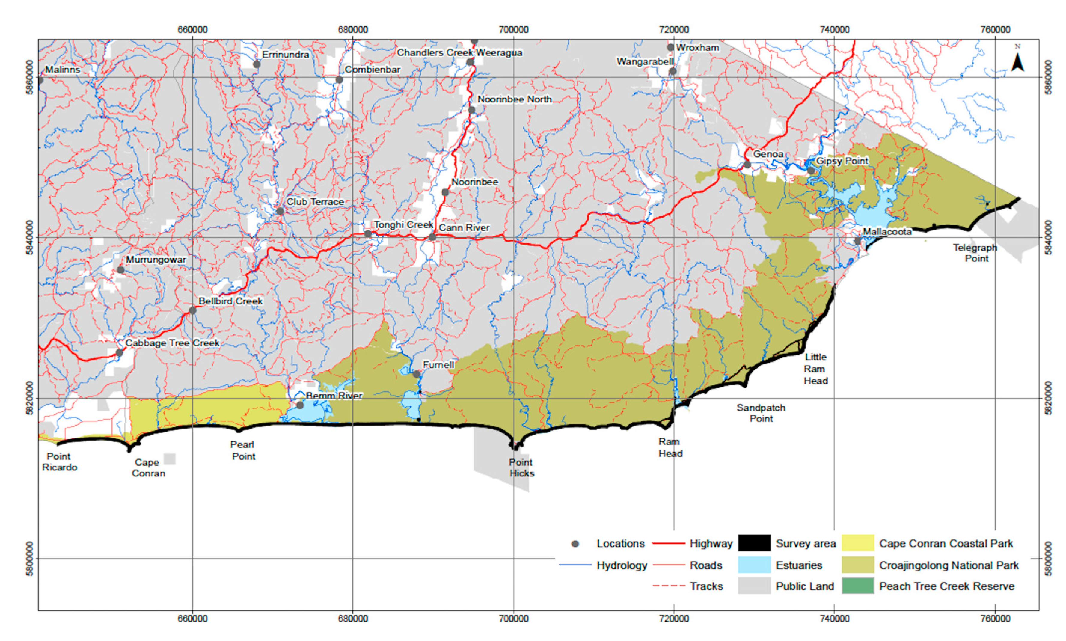
Figure 2.
The machine generated (TAN) local BN from the survey data. Each box or node represents a variable noted in the field (tables 1 & 2). The classes (continuous data) or states (for discrete data) for that variable appear within the box and show the occurrence in percentage. The lines connecting the boxes show the correlations observed in the data and indicate that one variable has an effect on another.
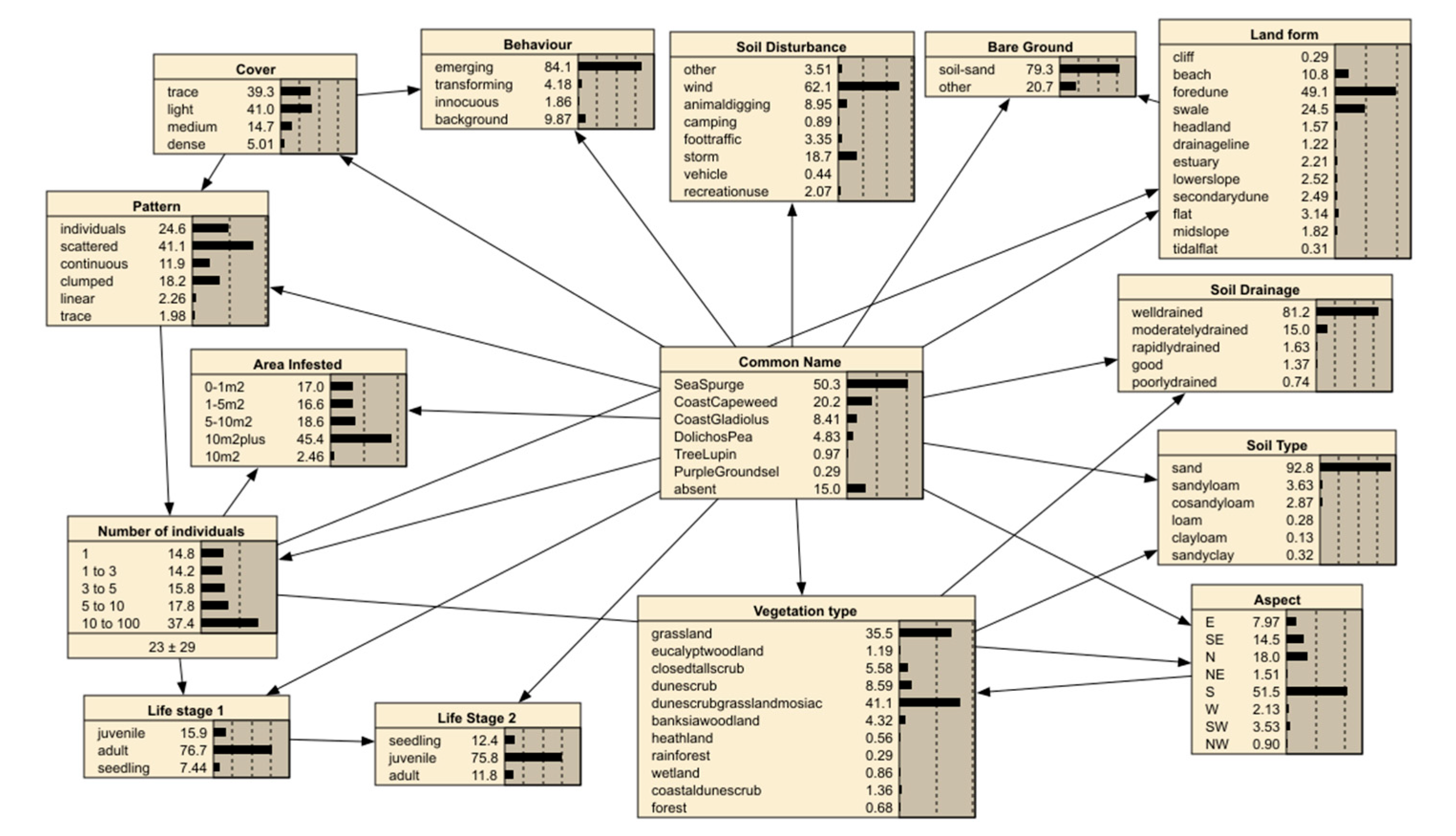
Figure 3.
The regional BN parameterized for Coastal Capeweed showing marginal probabilities for factors outlined in Table 3.
Figure 3.
The regional BN parameterized for Coastal Capeweed showing marginal probabilities for factors outlined in Table 3.
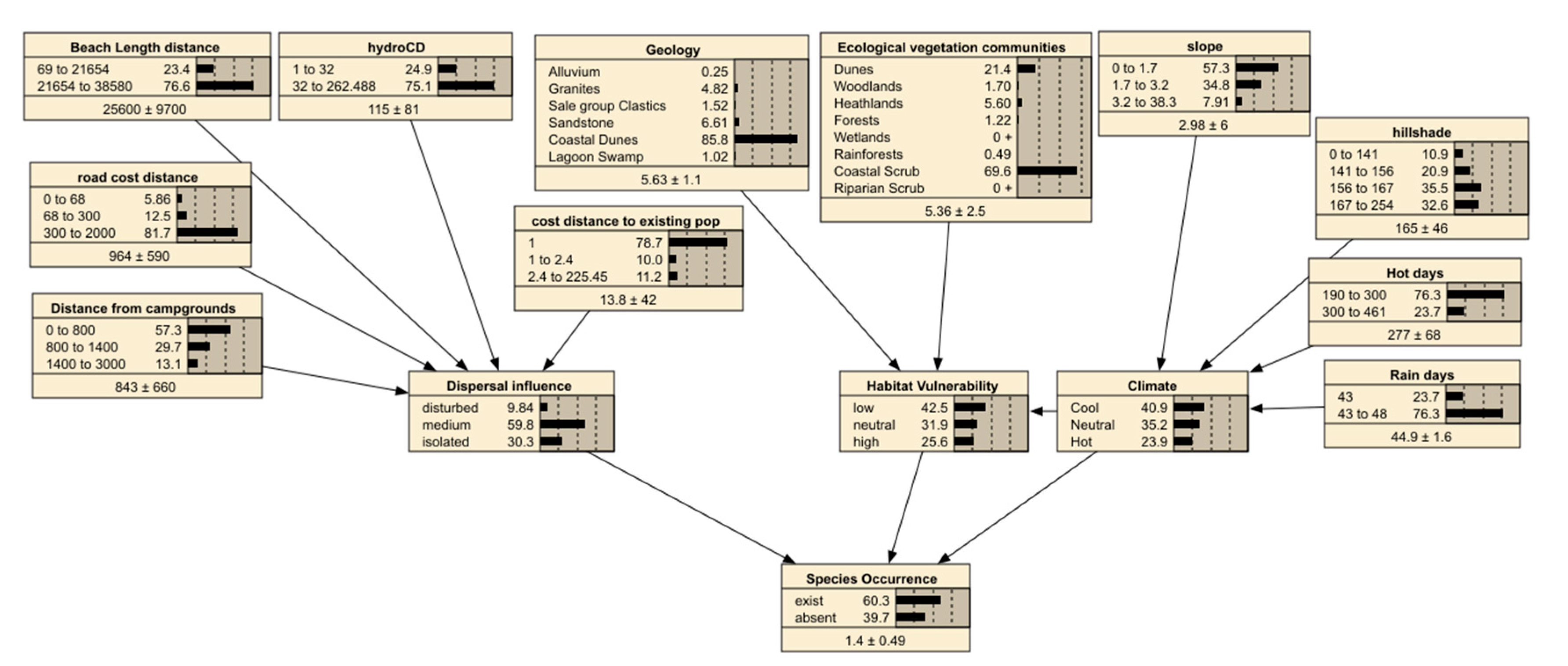
Figure 4.
The predicted likelihood of the Coastal Capeweed occurrence across the study region. Areas away from the survey locations have a low level of confidence. Inset map: Zoomed in section of the predicted model for Coastal Capeweed. The red regions indicate the high likelihood of observing the weed.
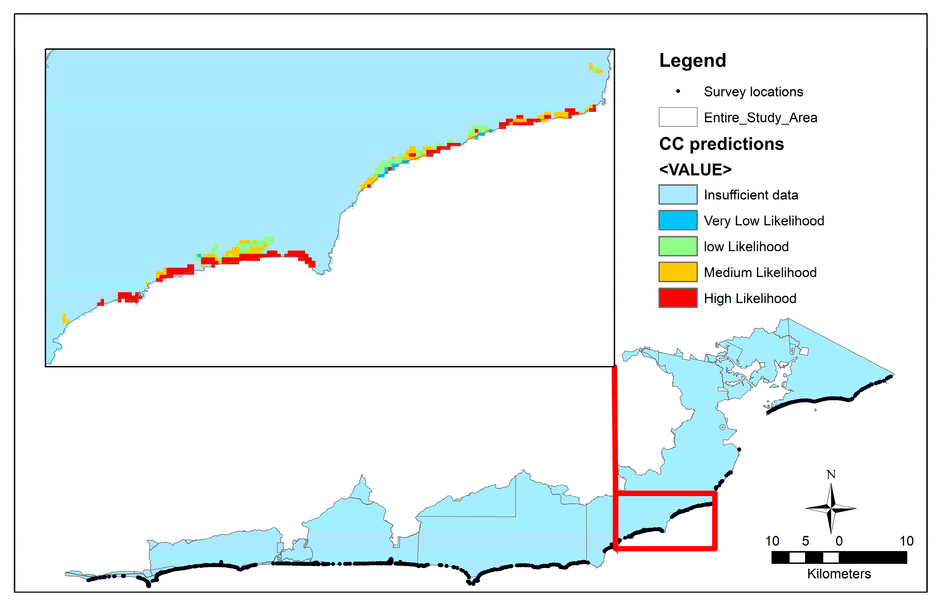
Table 1.
Weed Field Data Attributes Collected.
| Category | Attribute |
| Date Recorded | x/x/xx |
| Weed Common Name | Weed Common Name |
| Weed Scientific Name | Weed Scientific Name |
| Cover or Density of Weed | trace, light, medium, dense |
| Pattern of Infestation | scattered, clumped, linear, individuals, continuous |
| Life Stage | seedling, juvenile, adult |
| Number of plants | Optional |
| Area of Infestation | Optional |
| Weed Behaviour | innocuous, background, emerging, transforming |
| Landform | Fore dune, swale, primary dune, secondary dune, flat, mid slope, lower slope, upper slope, headland, cliff, drainage line, tidal flat, estuary |
| Vegetation Type | Wetland, rainforest, grassland, forest, eucalypt woodland, dune scrub grassland mosaic, dune scrub, closed tall dune scrub, banksia woodland, heathland |
| GPS location | Generated by GPS |
| High Threat | Yes/no |
| Comments |
Table 2.
Additional Weed Field Data Attributes Collected.
| Category | Attribute |
| Soil Type | Sand, loam, clay, sandy loam, clay loam, silty loam, silty clay |
| Soil Drainage | Poorly Drained, Moderately Drained, Good Drainage, Rapidly Drained |
| Soil Disturbance | Animal digging, campsite, flood, foot traffic, recreational use, roadside verge, storm, wind, other |
| Aspect | N, S, E, W |
| Vegetation Disturbance | Ground layer, mid layer, canopy or upper layer or none |
| Event | Storm, fire, flood, logging, disease/insect, none |
| Fire Frequency | Less than 5 years ago, greater than 5 years ago, none evident |
| Fire Comment | Provide comment on intensity of fire if recent |
| Bare Ground | Rock, soil/sand, leaf litter, lichen/moss, track or verge, campsite, recreation area, other |
| Other Comments |
Table 3.
GIS layers used to inform the model were sourced from Victorian Department of Environment, Land, Water and Planning (DELWP) and Bureau of Meterology (BOM) unless otherwise stated.
Table 3.
GIS layers used to inform the model were sourced from Victorian Department of Environment, Land, Water and Planning (DELWP) and Bureau of Meterology (BOM) unless otherwise stated.
| BN node | Spatial data | Description | Bin classes |
| Distance from Campground | DELWP Campgrounds and picnic areas layer | Distance in metres from the campground centre points | 0,800,1400,3000m |
| Road cost distance | DELWP roads layer | Euclidean distance from public roads | 0,68,300,2000m |
| Beach length distance | Coastline layer split up for each continuous beach section. | The length of uninterrupted beach for areas 500m from the beach | 213,21654,38580m |
| hydroCD | DELWP hydrological layer | Distance from rivers, creeks and inlets | 0,90,250m |
| Geology | Seamless Geology Victoria - 2014 EDITION, Geoscience Victoria |
Geology layer reclassified into 6 broadscale classes | Grouped classes |
| Ecological vegetation communities | DELWP EVC layer updated to include recent dune layer. | The Ecological Vegetation Communities layer classified into 8 classes. | Grouped classes |
| slope | DELWP Victorian DEM modelled to derive slope | Slope modelled from the Victorian DEM. | 0,1.7,3.2,38.3 degree |
| hillshade | DELWP Victorian DEM modelled to derive hillshade | Hill aspect modelled from the Victorian DEM | 0,141,156,167,254 degrees |
| Hot/cool days | BOM Average annual heating and cooling degree days. Pixel size:10728.4,10728.4m |
The number of degree days under 12 degrees in a year | 190,230,450 days |
| Rain days | BOM Average annual rainfall. Pixel size:10728.4,10728.4m | The average number of days exceeding 3mm of precipitation in a year | 43,45,48 days |
| Cost distance to existing pop | Field survey point data 2015 & 2016 | Distance from the observations of weed occurrence for 2015 and 2016 in 30x30m pixel units | 1,1.4,31.1 (30, 42 & 933metres) |
| Species Occurrence | Ethos NRM survey 2016, Ecosystems Management Pty Ltd 2015 survey | Observations of a specific weed and where absent | Variable depending on the weed |
Table 4.
Confusion Matrix showing the cases where the predicted (columns) occurrences are shown against the observed field data (rows) for the local BN. The diagonal column is the optimal location of the predictions that match observed.
Table 4.
Confusion Matrix showing the cases where the predicted (columns) occurrences are shown against the observed field data (rows) for the local BN. The diagonal column is the optimal location of the predictions that match observed.
| Predicted | |||||||
| Sea Spurge | Coast Cape weed | Coast Gladiolus | Dolichos Pea | Tree Lupin | Purple Ground Sel | absent | Actual |
| 138 | 5 | 11 | 0 | 1 | 0 | 0 | Sea Spurge |
| 11 | 48 | 7 | 0 | 0 | 0 | 0 | Coast Capeweed |
| 6 | 2 | 20 | 0 | 0 | 0 | 0 | Coast Gladiolus |
| 0 | 0 | 0 | 13 | 0 | 0 | 0 | Dolichos Pea |
| 1 | 0 | 0 | 0 | 4 | 0 | 0 | Tree Lupin |
| 0 | 0 | 0 | 0 | 0 | 0 | 0 | Purple Groundsel |
| 17 | 2 | 0 | 2 | 0 | 0 | 22 | absent |
Table 5.
Sensitivity of the weed list node ‘Common Name’ to a finding at another node for the local BN using variance reduction algorithm. The higher the variance percentage implies a higher influence on the Weed species occurance prediction.
Table 5.
Sensitivity of the weed list node ‘Common Name’ to a finding at another node for the local BN using variance reduction algorithm. The higher the variance percentage implies a higher influence on the Weed species occurance prediction.
| Node | Percent reduction in variance |
| Vegetation type | 29.2 |
| Behaviour | 22.8 |
| Soil Disturbance | 21.3 |
| Land form | 20.3 |
| Life Stage 1 | 12.6 |
| Aspect | 12.3 |
| Soil Drainage | 12.0 |
| Pattern | 11.8 |
| Bare Ground | 11.5 |
| Num Individuals | 11.3 |
| Life Stage 2 | 8.8 |
| Soil Type | 8.5 |
| Area infested | 6.9 |
| Cover | 5.2 |
Table 6.
Accuracy for each weed variation of the regional vulnerability BN model based on the confusion matrix. Accuracy testing using a 20% sample was not possible for weeds with low numbers and is indicated by Not Available (NA). The error rate is based on the ratio of correctly predicted cases verses the observed cases. The Gini coefficient varies in the range 0 to 1 where a value of 0 represents complete uncertainty and 1 represents complete certainty. AUC values range [0,1], where 1 denotes no error, 0.5 denotes totally random models, and <0.5 denotes models that more often provide wrong predictions [26].
| Weed species | Number of observations |
Error rate | Gini Coeff | AUC |
| Coastal Capeweed | 262 | 5.95% | 0.93 | 0.89 |
| Coastal Gladiolus | 87 | 6.12% | 0.88 | 0.94 |
| Dolichos Pea | 98 | 3.92% | 0.99 | 0.99 |
| Purple Groundsel | 3 | NA | NA | NA |
| Tree Lupin | 10 | NA | NA | NA |
| Sea Spurge | 1906 | 4.61% | 0.71 | 0.89 |
Table 7.
The Sensitivity of ‘Species Occurrence’ to a finding at another node in the regional vulnerability BN measured as percentage variance reduction.
Table 7.
The Sensitivity of ‘Species Occurrence’ to a finding at another node in the regional vulnerability BN measured as percentage variance reduction.
| Node | Coastal Gladiolus | Coastal Capeweed | Dolichos Pea | Purple Groundsel | Tree Lupin | Sea Spurge |
| Climate | 15.1 | 11.6 | 9.7 | 2.92 | 5.6 | 0 |
| Habitat vulnerability | 0.3 | 4.9 | 1.2 | 0.7 | 0.4 | 0 |
| Hot days | 0.9 | 0.4 | 0 | 0 | 0.2 | 0 |
| Rain days | 0.9 | 0.4 | 0 | 0 | 0.2 | 0 |
| Cost distance to existing population | 13.5 | 35.3 | 15 | 0.3 | 8.2 | 37.6 |
| Dispersal influence | 42.1 | 67 | 54.6 | 15.6 | 55.7 | 99 |
| EVC group | 1.1 | 1.3 | 0.5 | 0.4 | 0 | 0 |
| Beach Length distance | 6.2 | 1.4 | 0.4 | 0.3 | 0 | 0.6 |
| Geology | 0.3 | 0.3 | 0.6 | 0 | 0.1 | 0 |
| Camp distance | 1.0 | 0.7 | 0.3 | 0.3 | 0.7 | 0.9 |
| Hydro distance | 0.1 | 5.6 | 2.8 | 0 | 5.2 | 0 |
| slope | 0.1 | 0.1 | 0.1 | 0 | 0.1 | 0 |
| hillshade | 0.4 | 0.6 | 0.1 | 0 | 0.1 | 0 |
| Road cost distance | 1.7 | 1.0 | 0 | 1.3 | 1.3 | 0.1 |
Disclaimer/Publisher’s Note: The statements, opinions and data contained in all publications are solely those of the individual author(s) and contributor(s) and not of MDPI and/or the editor(s). MDPI and/or the editor(s) disclaim responsibility for any injury to people or property resulting from any ideas, methods, instructions or products referred to in the content. |
© 2024 by the authors. Licensee MDPI, Basel, Switzerland. This article is an open access article distributed under the terms and conditions of the Creative Commons Attribution (CC BY) license (http://creativecommons.org/licenses/by/4.0/).
Copyright: This open access article is published under a Creative Commons CC BY 4.0 license, which permit the free download, distribution, and reuse, provided that the author and preprint are cited in any reuse.


