Submitted:
06 July 2024
Posted:
08 July 2024
Read the latest preprint version here
Abstract
This study investigates the impact of Government Consumption (GC) on Saudi Arabia’s GDP during major economic crises from 1969 to 2022, with a focus on periods marked by fluctuations in oil and non-oil revenues. By integrating these revenue streams, the research provides a more comprehensive analysis of fiscal policy effectiveness during economic downturns. Using an Autoregressive Distributed Lag (ARDL) model, the study reveals the complex role of Government Consumption (GC) in stabilizing and stimulating the Saudi economy amidst revenue volatility.Key findings indicate that while GC does not significantly influence GDP in the short term, its long-term effectiveness varies across different crises. Specifically, GC has acted as a buffer against immediate economic shocks during certain crises while providing a stimulus for economic recovery in others. For instance, during the 2020 COVID-19 pandemic, timely fiscal measures significantly boosted GDP, underscoring the importance of adaptive and proactive fiscal policies. Conversely, the 2014-2016 oil price collapse demonstrated that GC alone was insufficient to counteract economic downturns, emphasizing the need for diversified revenue strategies.These findings underscore the dual role of GC in economic stabilization and recovery. During the COVID-19 pandemic, GC played a crucial role in both mitigating negative economic impacts and supporting recovery efforts, showcasing its effectiveness in times of global disruptions. This demonstrates GC's capability as an immediate buffer against economic shocks and a stimulus for economic recovery. In contrast, during the 2014-2016 oil price collapse, GC was less effective, indicating the limitations of relying solely on government spending without broader economic diversification. This highlights the necessity of diversified revenue strategies to complement fiscal measures for long-term economic resilience.The robustness of the findings was ensured through various diagnostic tests, including checks for autocorrelation, heteroskedasticity, and stationarity of residuals. The absence of significant autocorrelation and heteroskedasticity, along with the stationarity of differenced variables, confirms the validity of the econometric models used.The study contributes to the discourse on fiscal policy in oil-dependent economies by illustrating the critical role of diversified revenue strategies and adaptive fiscal measures in enhancing economic resilience. Recommendations are offered for policymakers to optimize fiscal strategies, ensuring robust economic recovery and long-term stability in volatile markets. This research highlights the necessity for Saudi Arabia to refine its fiscal policies towards greater economic diversification and stability.
Keywords:
Saudi Arabia
; oil revenues
; non oil revenues
; economic resilience
; fiscal policy
; oil-dependent economies
; economic diversification
Introduction
In oil-dependent economies, fiscal policy plays a pivotal role in mitigating economic volatility and fostering stability. Theoretical understanding in this context refers to the economic principles that explain how fiscal policies, like government consumption (GC), help stabilize an economy, particularly during downturns. This understanding is especially pertinent to Saudi Arabia, where oil revenues form the backbone of government income and are highly sensitive to market volatilities.
Economic stability and growth remain pivotal concerns for such national economies, particularly during periods marked by significant geopolitical and economic disruptions. Historical events such as the 1973 Oil Crisis, the 1980s Oil Glut, the 1990-1991 Gulf War, various oil price crashes (1998, 2008, 2014-2016), and the 2020 coronavirus pandemic have tested Saudi Arabia’s economic resilience. These events have underscored the vulnerabilities inherent in an oil-dependent economy and have catalyzed efforts towards economic diversification.
For instance, the Gulf War highlighted geopolitical risks that impacted oil production and prices, leading to broader economic implications. Similarly, severe drops in oil prices due to global oversupply and diminished demand in 1998 and 2008 severely impacted Saudi Arabia’s fiscal position, prompting the kingdom to earnestly pursue economic reforms and diversification strategies. The 2014-2016 oil price slump further exacerbated these challenges, leading to significant budget deficits and catalyzing substantial economic reforms under Vision 2030. This strategic initiative aims to diversify the economy and reduce oil dependency through comprehensive socio-economic reforms across various sectors. However, the sudden economic shock brought by the COVID-19 pandemic tested the resilience and efficacy of these ongoing economic transformations, impacting not only the oil sector but also the nascent tourism industry.
During such times, the role of fiscal policies, especially GC, becomes crucial in mitigating economic downturns. This study extends beyond the traditional scope of GC analysis by incorporating oil and non-oil revenues, significant drivers of economic activity, to dissect their combined impact on GDP. By doing so, it connects the specific historical and economic challenges faced by Saudi Arabia with the broader theoretical discourse on the role of fiscal policy in oil-dependent economies, highlighting how strategic fiscal management and diversification are essential for stabilizing and stimulating economic growth amidst external shocks and market fluctuations. The analysis reveals that GC exhibits varying effectiveness as both a buffer against immediate economic shocks and a stimulus for economic recovery, depending on the nature of the crisis.
Notably, while the 2020 COVID-19 pandemic showed significant positive impacts on GDP due to GC, highlighting the importance of timely and effective fiscal measures, the 2014-2016 oil price collapse demonstrated a significant negative impact, indicating the ineffectiveness of GC during that period.
High oil prices typically lead to budget surpluses, while low prices can swiftly turn these into significant deficits. To manage these fluctuations, oil-dependent countries often establish stabilization funds, also known as sovereign wealth funds, crucial for maintaining economic stability during periods of low oil prices by enabling the government to sustain spending without drastic cuts.
Moreover, the implementation of counter-cyclical fiscal policies—where savings are made during boom periods and spent during downturns—is considered ideal for such economies. However, the practical application of these policies can be challenging due to political pressures to increase spending or reduce taxes when oil revenues are high, often leading to pro-cyclical fiscal behaviors that exacerbate economic fluctuations rather than stabilizing them.
This study investigates the the impact of GC on real GDP in Saudi Arabia during major economic crises from 1969 to 2022, focusing on periods marked by fluctuations in oil revenues. By integrating oil and non-oil revenue streams, the research provides a more comprehensive understanding of fiscal policy effectiveness during economic downturns. Using ARDL model, the study reveals mixed results regarding the role of GC in stabilizing and stimulating the Saudi economy amidst revenues volatility. By examining both short-term and long-term effects, the research aims to understand how fiscal policies and revenue sources impact Saudi Arabia’s real GDP. Specifically, the research seeks to answer: How does Government Consumption influence GDP in Saudi Arabia during significant fluctuations in oil revenues? Are the existing fiscal policies effective in stabilizing the economy during downturns and stimulating recovery post-crisis? What strategic fiscal policy recommendations can be derived from the analysis to enhance economic resilience and stability in Saudi Arabia?
The discussion on the role of fiscal policies in stabilizing and diversifying the economy, as well as managing public debt and addressing social and political challenges, forms a critical theoretical foundation for understanding the complex interplay between fiscal management and economic performance in oil-dependent countries. Integrating both oil and non-oil revenue streams, this study highlights the role of GC in managing economic fluctuations and supporting long-term growth. By examining these aspects, the study aims to contribute valuable insights into the formulation of more resilient economic strategies for Saudi Arabia. The insights include the effectiveness of government consumption in mitigating the adverse effects of economic downturns, the need for adaptive fiscal policies to manage revenue volatility, and the importance of diversifying revenue streams to reduce dependence on oil revenues and enhance economic stability. Additionally, the study provides recommendations on optimizing public investments to stimulate long-term economic growth and guidelines for policymakers to design fiscal policies that can buffer the economy against cyclical fluctuations and promote sustainable growth. These insights are crucial for policymakers aiming to enhance economic stability and growth in the face of both global and local economic challenges.
2. Literature Review: Theoretical Backdrop of Counter-Cyclical Fiscal Policies
Counter-cyclical fiscal policies are designed to stabilize the economy by adjusting government spending and taxation in response to economic fluctuations. These policies aim to counterbalance the business cycle, mitigating adverse effects and promoting economic stability and growth. For instance, Luan, Man, and Zhou (2021) emphasize that fiscal policy can effectively complement monetary policy to stabilize macroeconomic conditions by influencing aggregate demand and addressing economic downturns. They found that coordinated fiscal and monetary policies lead to more robust macroeconomic stability, especially during periods of economic uncertainty. Similarly, Shaheen (2019) examines how government expenditure and tax policies influence private consumption and labor supply. Shaheen’s findings indicate that increased government spending positively affects private consumption and labor supply, leading to higher overall economic activity.
Keynesian Theory and Automatic Stabilizers
According to Keynesian theory, aggregate demand plays a crucial role in determining economic output and employment levels. Counter-cyclical fiscal policies manage aggregate demand by increasing government spending and reducing taxes during economic downturns to boost demand and by decreasing spending and increasing taxes during economic expansions to prevent overheating (Bravo & Ayuso, 2021). Moreover, automatic stabilizers are fiscal mechanisms that naturally counterbalance economic fluctuations without additional government action. Examples include unemployment insurance, which increases government spending during downturns as more people become eligible for benefits, and progressive taxation, where tax revenues fall during recessions as incomes drop, cushioning disposable incomes (Bongers & Díaz-Roldán, 2019).
Significance and Challenges of Counter-Cyclical Fiscal Policies
Bongers and Díaz-Roldán (2019) and Buendía-Martínez, Álvarez-Herranz, & Moreira Menéndez (2020) highlight the significance of counter-cyclical fiscal policies in maintaining economic stability and fostering sustainable growth. By boosting aggregate demand during downturns, these policies aim to reduce the depth and duration of recessions, while curbing demand during booms helps to prevent inflation and asset bubbles. Saudi Arabia’s Vision 2030 exemplifies the strategic use of fiscal policies to diversify the economy away from oil dependence, emphasizing the development of non-oil sectors such as tourism, entertainment, and technology. This ambitious plan involves significant fiscal reforms and strategic investments to enhance economic resilience.
However, the effectiveness of counter-cyclical fiscal policies often depends on the economic context, structural characteristics of the economy, and the initial fiscal position of the government. High levels of public debt can constrain a government’s ability to implement expansive fiscal policies due to the increased cost of borrowing and potential impacts on investor confidence. Thus, while the theoretical benefits of fiscal policy are widely recognized, practical implementation and outcomes can vary significantly across different economic environments.
Recent studies have emphasized the critical importance of designing fiscal policies with long-term sustainability in mind, complementing short-term counter-cyclical measures. Piroli and Calderón (2021) underscored this point in their analysis of fiscal sustainability in Central and Eastern European countries, highlighting the need to accumulate surpluses during economic booms to prepare for future downturns. Studies such as those by Auerbach and Gorodnichenko (2012) have demonstrated the variability of fiscal multipliers, showing that government spending can have different impacts on the economy depending on the state of the economic cycle.
Fiscal Policy in Oil- Dependent Economies
Fiscal policy in oil-dependent economies is characterized by its heavy reliance on oil revenues to fund government expenditures and stimulate economic growth. These economies often face unique challenges and vulnerabilities due to the volatility of oil prices, which can lead to fluctuations in government revenues and budget deficits. Policymakers in these economies often seek to diversify their economies away from oil, strengthen fiscal institutions, and improve the transparency and accountability of fiscal policy decisions.
Case Studies of Oil-Dependent Economies
Venezuela presents a stark example of the risks associated with high oil dependency. As detailed by Su, C. W., Khan, K., Tao, R., & Umar, M. (2020), Venezuela’s economic crises have been exacerbated by fiscal mismanagement and an inability to stabilize or diversify the economy away from oil. In contrast, Russia has managed its oil revenues more effectively. A study by Spilimbergo (2007) highlights Russia’s use of the Oil Stabilization Fund to manage oil revenue surges and maintain fiscal balance, mitigating potential fiscal imbalances. Byiabani and Mohseni (2014) explored the impact of fiscal policy on Iran’s economic growth from 1974 to 2007, showing that Iran’s long-term economic performance was influenced by various factors, including labor force and physical capital, alongside proactive fiscal measures such as tax reductions and increased government spending on development. Aghilifar, H., Zare, H., Piraei, K., & Ebrahimi, M. (2023) demonstrated that although Iran heavily relies on oil for its revenue, effective fiscal policies have been crucial in mitigating the impact of global price fluctuations and maintaining macroeconomic stability. Khosravi and Karimi (2010) further examined the relationship between fiscal and monetary policy and economic growth in Iran, revealing that while government expenditure had a significant positive impact on GDP growth, inflation, and exchange rates, components of monetary policy had a negative impact.
Similarly, the experiences of Oman, Saudi Arabia, and Bahrain underscore the importance of strategic economic planning and diversification. Studies by Aslam and Shastri (2019) and Hamdi & Sbia (2013) demonstrate the long-term and short-term impacts of oil revenues on GDP, emphasizing the need for these countries to diversify away from oil dependence. Khayati (2019) provides insights into the differential impacts of oil and non-oil exports on Bahrain’s economic growth, advocating for economic diversification to reduce volatility and promote sustainable development. Azmi (2013) supports this view by demonstrating the significant impact of government spending on economic metrics like GDP, interest rates, and unemployment in Malaysia, further reinforcing the multifaceted role of fiscal policies in economic management.
Moreover, Almarzoqi and Mahmah (2020) highlight the significance of non-oil revenue growth as a stabilizing factor for government consumption. Their evidence suggests that diversification efforts are beginning to mitigate the volatility associated with oil revenues. This aligns with the broader literature that underscores the importance of economic diversification in achieving sustainable growth and stability. By expanding into various sectors, Saudi Arabia can reduce its economic vulnerability to oil price fluctuations and enhance its fiscal resilience. This multi-faceted approach to diversification not only supports immediate economic stability but also lays the foundation for long-term growth and prosperity.
Strategic Fiscal Management and Diversification
Implementing counter-cyclical fiscal policies and integrating oil and non-oil revenue streams into the fiscal policy framework can help stabilize the economy and reduce dependence on oil. This approach is supported by studies from various countries, highlighting the importance of strategic fiscal management and diversification. Case studies highlight the importance of strategic fiscal management and the necessity for oil-dependent economies to diversify their revenue bases. Implementing counter-cyclical fiscal policies, such as those proposed by Blanchard and Leigh (2013), could potentially mitigate the adverse effects of revenue volatility. Additionally, integrating oil and non-oil revenue streams effectively into the fiscal policy framework, as shown in VAR models by Schmidt-Hebbel and Marshall (2007), can help stabilize the economy and reduce dependence on oil.
Building on this discussion, the literature further explores the relationship between national oil revenues and economic growth across various countries. In 2017, Nwoba and Abah examined the impact of oil revenues and the presence of multinational oil companies on economic growth in Nigeria. Their findings suggest that these factors play a vital role in driving economic growth, particularly through job creation. Furthermore, a study by Hassan and Abdullah (2015) investigated the impact of oil revenues on the output of the service sector in Sudan between 2000 and 2010, finding that oil revenues positively affected the sector’s output.
Strategic fiscal management in Saudi Arabia involves not only stabilizing the economy during oil price downturns but also actively promoting diversification. The Vision 2030 plan outlines substantial investments in infrastructure, education, and healthcare to create a more diversified economic base. Studies by Aslam and Shastri (2019) and Hamdi & Sbia (2013) emphasize the importance of such strategic economic planning and diversification efforts in ensuring long-term economic stability and growth. These studies collectively provide robust evidence of the diverse effects of oil revenues on economic growth in regions like Saudi Arabia, Nigeria, and Sudan. They underscore the nuanced ways in which oil-dependent economies can leverage their natural resources to achieve broader economic objectives, highlighting the need for carefully crafted fiscal policies that support sustainable development and diversification.
In exploring the trajectories of economic development and diversification, Gelb (2010) highlights the significant shift from primary commodity exports to industrial products in developing countries. The diversification into various industrial sectors not only stabilized their national incomes but also reduced economic volatility, contributing substantially to sustainable growth. This shift, according to Gelb, is indicative of successful integration into South–South trade and continuous enhancement of export sophistication.
Parallel to Gelb’s findings, Richard M. Auty (2001) has extensively explored the role of resource abundance in enhancing economic performance. Auty’s work emphasizes that while resource wealth can lead to economic advantages, strategic diversification is crucial to harness these benefits effectively and sustainably. His analysis suggests that countries with abundant resources can leverage this advantage to fuel broader economic development, but this requires deliberate policy efforts aimed at diversification into non-resource sectors to avoid the pitfalls of over-reliance on volatile resource markets. This perspective is crucial for understanding the complex dynamics between natural resource wealth and long-term economic stability.
Fiscal policies play a fundamental role in supporting diversification efforts, as noted by the World Bank (2019). Strategic government spending and tax incentives can encourage investments in non-oil sectors like manufacturing, agriculture, and services, thereby broadening the economic landscape. Countries such as Saudi Arabia and the UAE have utilized fiscal initiatives like the development of economic cities, investment in renewable energy projects, and labor law reforms to promote economic diversification. These policies aim to attract foreign direct investment, stimulate private sector growth, and create a more resilient economic environment.
The literature also suggests that while the immediate benefits of diversification may be gradual, the long-term effects are significantly positive. Diversified economies tend to exhibit more stable economic conditions during oil downturns. However, the effectiveness of these strategies often relies on the consistent implementation of supportive fiscal policies and the overall political and economic stability of the country. Therefore, policymakers are encouraged to consider comprehensive fiscal reforms that align with broader economic diversification goals to ensure sustainable development and economic stability.
Fiscal Policy in Saudi Arabia
The fiscal policy in Saudi Arabia has traditionally been heavily reliant on oil revenues. As highlighted by Al Rasasi, Qualls, and Alghamdi (2019), oil revenues have a strong link to both short- and long-term economic growth in the country. However, the volatility of oil prices poses a significant challenge to fiscal stability. The Saudi government has implemented various measures to mitigate this volatility, including the establishment of the Public Investment Fund (PIF) to manage and invest oil revenues strategically. Saudi Arabia’s Vision 2030 aims to diversify the economy away from oil dependence, emphasizing the development of non-oil sectors such as tourism, entertainment, and technology. This ambitious plan involves significant fiscal reforms and strategic investments to enhance economic resilience.
Government Spending and Economic Stability
Government spending is a critical component of fiscal policy with significant implications for economic growth and stability. Barro (1990) and Cavallo (2005) provide a comprehensive analysis of the effects of government expenditure on economic growth, concluding that while strategic public spending can promote growth, excessive expenditure may lead to inefficiencies and diminished economic performance. These insights are particularly relevant in the context of Saudi Arabia, where government consumption has been a key tool for economic stabilization, especially during periods of revenue volatility. However, excessive expenditure without corresponding revenue diversification can lead to inefficiencies and economic instability. The Saudi government’s focus on efficient allocation of resources to productive sectors is essential in this context.
The interplay between fiscal policies and their economic impacts is critical, with government expenditures significantly shaping economic outcomes. Foundational studies by Cavallo (2005) and Tulsidharan (2006) examine the effects of government expenditure on economic stability and growth, particularly in India, setting the stage for a detailed exploration of GC and its role during financial crises. Similarly, Kira (2013) highlights the significant role of government and household consumption in influencing GDP in developing countries like Tanzania, underscoring the importance of fiscal measures in driving economic output.
Fiscal Multipliers and Economic Recovery
Empirical studies illustrate that General Consumption (GC) acts as a stabilizer during downturns by buffering cyclical fluctuations and supporting demand. For instance, Auerbach and Gorodnichenko (2012) demonstrate the variability of fiscal multipliers of GC across business cycles, highlighting increased effectiveness during recessions. This is particularly notable in sectors directly linked to government spending, such as healthcare and infrastructure, where Blanchard & Leigh (2013) observed enhanced benefits. Drawing on historical crises, the literature suggests prioritizing GC in fiscal strategies for rapid and effective economic recovery, supported by empirical evidence from past events like the 2008 financial crisis (Bernanke, 2015).
Institutional Quality and Fiscal Policy Effectiveness
Structural reforms and institutional strengthening are vital for effective public debt management. Fatai et al. (2017) emphasize that institutional quality, including effective governance and anti-corruption measures, significantly influences fiscal outcomes. Strong fiscal institutions provide a stable framework for policy implementation, ensuring sustainable debt management. Empirical studies, such as those by Aslam and Shastri (2019) and Hamdi & Sbia (2013), demonstrate the long-term benefits of strategic fiscal planning and diversification in countries like Oman, Saudi Arabia, and Bahrain. These studies show that well-managed fiscal policies can help stabilize economies and reduce debt burdens, even in the face of oil revenue volatility.
The effectiveness of fiscal policy is significantly influenced by the quality of institutions. Efayena and Olele (2024) explore this moderating effect in Sub-Saharan Africa, demonstrating that good governance and robust institutions enhance the positive impacts of fiscal policies on economic growth. This finding is particularly relevant for Saudi Arabia as it pursues institutional reforms under Vision 2030. By strengthening governance frameworks and ensuring transparent and efficient public spending, Saudi Arabia can maximize the benefits of its fiscal policies and support long-term economic growth and stability. High-quality institutions are essential for translating fiscal measures into tangible economic benefits, while weak institutions can undermine these efforts.
Impact of Oil Revenue Volatility on Fiscal Policies
Building on the discussion of fiscal responsiveness, the literature also delves into the significant impact of oil revenue volatility on the fiscal policies of oil-dependent countries. A pivotal study by Sohag, Kalina, and Samargandi (2024) explores this dynamic interplay between oil price fluctuations and fiscal policies in OPEC+ member countries. The authors employ advanced econometric tools such as Hodrick-Prescott and Hamilton filters to isolate cyclical components of oil prices, enhancing the analysis through a Panel VAR approach under a system GMM framework.
Their findings reveal that cyclical oil price shocks have an immediate, positive impact on the fiscal stances of these countries, though the effects tend to diminish over the medium to long term. Interestingly, gradual oil price trends show an insignificant impact on fiscal policies, suggesting that OPEC+ countries’ fiscal strategies are more responsive to abrupt changes rather than gradual shifts in the oil market. The study highlights the disparate capabilities among OPEC+ countries, such as Gabon, Iraq, Russia, Saudi Arabia, the UAE, and Kazakhstan, to leverage these shocks for economic advantage. This differentiation is critical as it illustrates the varied economic resilience within the alliance, informing tailored policy formulations aimed at enhancing fiscal stability and growth.
Further contributing to our understanding of the fiscal dynamics in oil-dependent economies, Fatai, Liu, Adeniyi, and Kabir (2017) utilize a panel dataset from 2000 to 2015 to empirically examine the relationship between crude oil rents and fiscal balance. Their findings suggest that in countries with fiscal rules, the reaction of fiscal balance to oil rent shocks is weak and statistically insignificant. They also highlight factors such as welfare spending, the debt-to-GDP ratio, and the government’s effectiveness in curbing corruption and mismanagement, which significantly influence fiscal balance.
Integrating Government Consumption and Economic Resilience
Integrating these insights, it becomes clear that strategic fiscal management and diversification are essential for stabilizing and stimulating economic growth amidst external shocks and market fluctuations. Government consumption (GC) plays a crucial role in this context. The literature underscores that GC acts as a stabilizer during downturns by buffering cyclical fluctuations and supporting demand, particularly in sectors directly linked to government spending such as healthcare and infrastructure.
Empirical Insights on Fiscal Policy During Economic Crises
Recent research has provided valuable insights into the dynamics of fiscal policy and its impact on economic stability. Meisenbacher and Wilson (2023) explore the role of fiscal policy during the COVID-19 pandemic and highlight how government spending significantly influenced economic recovery. Their study indicates that substantial fiscal expansion during the pandemic recession, characterized by large government expenditures and transfers, contributed to real economic growth. This finding underscores the importance of discretionary fiscal measures in mitigating economic downturns and stimulating recovery. The study also notes that U.S. fiscal policy is projected to be neutral in the near term, neither significantly stimulating nor constraining economic growth, highlighting the nuanced role of fiscal interventions in different economic contexts. These insights align with the broader narrative of our study, emphasizing the critical role of timely and substantial fiscal measures in enhancing economic resilience, especially during periods of crisis.
Impact of Fiscal Policies During Economic Crises
Caselli et al. (2023) discuss how exceptional economic conditions since the pandemic have shaped fiscal outcomes, calling for consistent policies to address inflation, safeguard public finances, and protect the most vulnerable. These findings inform our analysis of Saudi Arabia’s fiscal policy adjustments post-pandemic and their implications for economic resilience. The need for timely and substantial government interventions during crises is further underscored by the contrasting impacts observed during the 2014-2016 oil price collapse and the 2020 COVID-19 pandemic.
Contributions of the Present Study
By reviewing the literature, the present study makes significant contributions to the existing body of knowledge on fiscal policy and economic resilience in oil-dependent economies. It provides a comprehensive longitudinal analysis of Saudi Arabia’s Vision 2030, tracking progress and outcomes over time to evaluate the effectiveness of fiscal reforms and diversification strategies. By documenting key milestones, the study offers insights into policy evolution and their long-term impacts on economic stability and growth, identifying trends and assessing policy effectiveness. Additionally, it presents robust empirical evidence on the impact of diversification efforts by analyzing data on government spending, revenue streams, and economic outcomes. This approach evaluates how diversification contributes to fiscal stability and long-term resilience, highlights practical outcomes, informs future policy decisions, and offers a model for other oil-dependent economies. The study underscores the importance of data-driven insights in reducing economic vulnerability to oil price fluctuations and achieving sustainable growth.
3. Methodology
This study investigates the impact of Government Consumption (GC), Oil Revenues (OR), and Non-Oil Revenues (NOR) on Saudi Arabia’s GDP during major economic crises from 1969 to 2022. ARDL model is employed to analyze the short-term and long-term effects of these variables on GDP. The theoretical framework is informed by Keynesian economic principles, which postulate that GC can play a stabilizing role in the economy, especially during periods of downturn. This effect is particularly crucial in an oil-dependent economy like Saudi Arabia, where revenue streams are highly volatile and susceptible to external shocks in the global oil market.
GC is expected to counteract economic fluctuations by directly injecting funds into the economy, thus sustaining employment and consumption during downturns. The role of GC becomes critical in managing the cyclical nature of oil revenues, which are prone to cause economic instability due to their sensitivity to global oil price fluctuations. Moreover, the inclusion of non-oil revenues, which may arise from sectors such as tourism, manufacturing, and services, helps assess the effectiveness of economic diversification efforts and their role in fiscal stability. These revenues, often promoted through fiscal incentives, exhibit different dynamics from oil revenues and contribute to overall economic resilience, balancing the instability of oil-dependent financial streams.
3.1. Data
The primary data, collected annually, is sourced from the Saudi Arabian Monetary Agency (Saudi Central Bank) (SAMA), the World Bank, and the Ministry of Finance. This ensures a robust dataset that reflects the key economic activities impacting the Saudi economy. The analysis uses several key economic variables: Real Gross Domestic Product (GDP), Real Government Consumption (GC), Real Oil Revenues (OR), and Real Non-Oil Revenues (NOR). All variables are converted to real values using the Consumer Price Index (CPI) to adjust for inflation, enabling consistent comparison over time.
3.2. Model Specification
The study employs the ARDL model for analyzing the long-run and short-run relationships between the variables. The ARDL model is chosen for its flexibility in handling variables with different integration orders (I(0) and I(1)) and its ability to provide unbiased long-run estimates even with small sample sizes. This model helps in understanding both the immediate impacts of fiscal policy changes and the long-term equilibrium relationships among the variables. The ARDL model equation used is as follows:
Where:
ΔGDPt=α0+∑i=1pαiΔGDPt−i+∑i=0qβiΔGCt−i+∑i=0rγiΔORt−i+∑i=0sδiΔNORt−i+λ1GDPt−1+λ2GCt−1+λ3ORt−1+λ4NORt−1+ϵtΔGDPt=α0+∑i=1pαiΔGDPt−i+∑i=0qβiΔGCt−i+∑i=0rγiΔORt−i+∑i=0sδiΔNORt−i+λ1GDPt−1+λ2GCt−1+λ3ORt−1+λ4NORt−1+ϵt
- Δ denotes the first difference operator.
- t is the time period.
- GDP is the Gross Domestic Product in real values (adjusted using CPI).
- GC is Government Consumption in real values (adjusted using CPI).
- OR is Oil Revenue in real values (adjusted using CPI).
- NOR is Non-Oil Revenue in real values (adjusted using CPI).
- α0 is the intercept term.
- αi,βi,γi,δi are the short-run coefficients.
- λ1,λ2,λ3,λ4 are the long-run coefficients.
- ϵt is the error term.
3.3. Description of Variables
Gross Domestic Product (GDP): Represents the total market value of all final goods and services produced within a country in a given period. It serves as the dependent variable, reflecting the overall economic health and performance of the nation.
Government Consumption (GC): Refers to the total government expenditure on goods and services, excluding capital expenditures. GC directly impacts current consumption, making it essential for analyzing its role in stabilizing and stimulating economic activity during various crises. It provides a measure of the immediate impact on economic activity, aligning with Keynesian economic theory.
Oil Revenues (OR): These are revenues derived from the extraction and sale of oil, a significant source of income for Saudi Arabia, which directly impacts the fiscal policy and economic stability of the nation. Analyzing oil revenue helps identify how dependencies on volatile economic factors influence broader economic stability and the buffering role of fiscal policies like GC.
Non-Oil Revenues (NOR): Non-oil revenues refer to the income generated from economic activities that are not directly related to the oil sector. These revenues are crucial for Saudi Arabia’s economic diversification efforts, aimed at reducing the Kingdom’s reliance on oil income and fostering sustainable economic growth through various other sectors. Specifically, non-oil revenues include income from the export of goods and services produced in sectors such as manufacturing, agriculture, and services other than oil. Additionally, investment income from both domestic and foreign investments, including returns on investments in financial assets, real estate, and other sectors, contributes significantly. Consumer spending, reflecting the overall health of the domestic economy, also plays a vital role. Furthermore, revenues generated from private-sector activities, including those in rapidly growing industries such as arts and entertainment, food production, transport and storage, health and education, trade, restaurants, hotels, and communications, are pivotal to these diversification efforts.
3.3. Steps Involved
First, descriptive statistics are computed to summarize the key characteristics of the data. This is followed by the creation of a correlation matrix to identify the relationships between the variables. To ensure the validity of the regression results, the Augmented Dickey-Fuller (ADF) test is applied to check the stationarity of the variables. This step is crucial to avoid spurious regression results. Next, appropriate lag lengths are determined using criteria such as the Akaike Information Criterion (AIC) and the Schwarz Information Criterion (SIC). The ARDL bounds testing approach to cointegration is then employed to test for the existence of a long-run relationship between the variables. Subsequently, an Error Correction Model (ECM) is applied to describe short-term dynamics and the adjustment process towards long-term equilibrium.
The study also includes several diagnostic checks to ensure the robustness of the model. The Breusch-Godfrey LM test is conducted to detect the presence of autocorrelation in the residuals, while the ARCH test is used to check for heteroskedasticity or changing variance in the residuals over time. To ensure there is no severe multicollinearity among the independent variables, the Variance Inflation Factor (VIF) is utilized. The stability of the coefficients over the sample period is assessed using the CUSUM and CUSUM of Squares tests.
Sensitivity analysis is performed by conducting the ARDL analysis with and without dummy variables to account for the impact of specific economic crises. Finally, the model is re-estimated with interaction terms to analyze the impact of each crisis, by including interaction terms between the dummy variables and government consumption.
3.5. Focus on Specific Economic Crises
The study provides an in-depth analysis of the impact of Government Consumption (GC) on GDP during major economic crises, offering valuable insights into the effectiveness of fiscal policies in stabilizing and stimulating the economy. By examining these crises, we can better understand the nuanced role that GC plays in mitigating economic shocks and fostering recovery. The identified crises include:
1973 Oil Crisis: Triggered by geopolitical tensions and an oil embargo, this crisis led to skyrocketing oil prices and global economic turmoil. Analyzing the role of GC during this period helps us understand how fiscal policies can buffer against supply shocks and inflationary pressures.
1980s Oil Glut: Characterized by an oversupply of oil, this period saw plummeting oil prices and significant economic disruptions for oil-exporting countries. Studying GC’s impact during this glut provides insights into the challenges and strategies for maintaining economic stability amid drastically reduced oil revenues.
1990 Gulf War: This conflict caused temporary disruptions in oil supply and heightened geopolitical risks. Examining GC during this period sheds light on the fiscal responses required to manage short-term economic shocks and maintain public confidence.
1997 Asian Financial Crisis: Originating from currency devaluation and financial instability in Asia, this crisis had global repercussions. Understanding GC’s role during this time offers perspectives on how fiscal policies can help economies withstand financial contagion and support recovery.
2000 Dot-com Bubble: The bursting of the speculative bubble in technology stocks led to a significant market downturn. Analyzing GC during this period highlights the importance of government spending in mitigating the effects of asset price collapses and supporting economic resilience.
2008 Financial Crisis: Triggered by the collapse of the housing market and financial institutions in the United States, this crisis caused widespread economic distress. Studying the impact of GC during this global recession provides crucial lessons on the role of counter-cyclical fiscal policies in promoting economic recovery.
2014-2016 Oil Price Collapse: Driven by a combination of oversupply and weakened demand, this period saw a steep decline in oil prices. Examining GC during this collapse emphasizes the need for diversified revenue strategies and the limitations of relying solely on government spending to counteract economic downturns.
2020 Coronavirus Pandemic: The COVID-19 pandemic led to unprecedented global economic disruptions. Analyzing GC during this crisis demonstrates the effectiveness of timely and substantial fiscal measures in supporting economic activity and mitigating the impacts of a global health emergency.
By focusing on these specific economic crises, the study not only contextualizes the role of GC within different types of economic disruptions but also highlights the importance of adaptive and proactive fiscal policies. This analysis is crucial for developing resilient economic strategies that can better withstand future shocks and promote sustainable growth.
4. Results
4.1. Descriptive Statistics
The descriptive statistics for the key variables (Real GDP, OIL Revenues, NON-OIL Revenues, and GOVT Consumption) over the sample period from 1969 to 2022 are summarized in the following table:

Table 1.
Descriptive Statistics of Key Economic Variables (1969-2022).
| Statistic | GDP (millions) | OR (millions) | NOR (millions) | GC (millions) |
| Mean | 1,195,328.0 | 40,915.5 | 84,800.2 | 282,450.7 |
| Median | 780,787.5 | 17,428.8 | 58,016.6 | 197,999.2 |
| Maximum | 3,212,168.6 | 670,265.0 | 319,357.7 | 844,957.0 |
| Minimum | 107,832.5 | 2,803.2 | 2,448.3 | 17,076.9 |
| Std. Dev. | 854,762.6 | 94,154.7 | 77,804.6 | 209,188.3 |
| Skewness | 0.8 | 5.8 | 1.8 | 0.8 |
| Kurtosis | 2.3 | 38.6 | 5.7 | 2.6 |
| Jarque-Bera | 6.5 | 3,145.0 | 46.3 | 5.6 |
| Probability | 0.0 | 0.0 | 0.0 | 0.1 |
| Sum | 64,547,711.2 | 2,209,435.9 | 4,579,211.2 | 15,252,340.1 |
| Sum Sq. Dev. | 3.87E+13 | 4.70E+11 | 3.21E+11 | 2.32E+12 |
| Observations | 54 | 54 | 54 | 54 |
The table above presents the descriptive statistics for key economic variables from 1969 to 2022.
GDP exhibits substantial variation, with values ranging from a minimum of 107,832.5 million to a maximum of 3,212,168.6 million, and an average of approximately 1,195,328.0 million. This indicates significant economic growth over the period, reflecting the overall expansion of the Saudi economy. The wide range of GDP values suggests periods of rapid economic growth, likely driven by oil booms and extensive government investments, as well as periods of economic downturns possibly due to oil price shocks or global economic recessions.
Oil revenues show extreme variability, with a maximum of 670,265.0 million and a minimum of 2,803.2 million. The high average of 40,915.5 million reflects the central role of oil in the Saudi economy. The high skewness (5.8) and kurtosis (38.6) indicate a non-normal distribution with frequent extreme values, underscoring the volatility of the global oil market. This volatility has significant implications for fiscal policy and economic stability.
Non-oil revenues also show substantial variation, with a mean of 84,800.2 million, a maximum of 319,357.7 million, and a minimum of 2,448.3 million. This reflects efforts towards economic diversification away from oil dependency. The positive skewness (1.8) and high kurtosis (5.7) suggest that while there have been periods of significant growth in non-oil sectors, these revenues still experience considerable fluctuations.
Government consumption ranges widely from 17,076.9 million to 844,957.0 million, with an average of 282,450.7 million. This indicates varying levels of public sector involvement and government spending in the economy. The variability in government consumption suggests periods of increased public spending, possibly during economic downturns or to stimulate growth, and periods of austerity or reduced spending.
Statistical Distributions: The skewness and kurtosis statistics for all variables indicate deviations from normality, particularly in oil revenues. This non-normality suggests that the economic variables have experienced periods of extreme values, reflecting the economic volatility and structural shifts over time.
Economic Volatility and Structural Shifts: The high variability and non-normality in oil revenues and other economic indicators highlight the volatility of the Saudi economy, primarily driven by fluctuating oil prices. This underscores the challenges of managing an oil-dependent economy. The data suggest structural shifts in the economy, particularly efforts to diversify income sources and reduce reliance on oil revenues. The variability in non-oil revenues and government consumption reflects these ongoing adjustments.
4.2. Correlation and Trend Analysis
The correlation matrix in Table 2 provides insights into the relationships between key economic variables: GDP, OR, NOR, and GC over the period from 1969 to 2022. The table shows strong positive relationships between GDP and GC (0.966) as well as between GDP and NOR (0.825). This suggests that as GDP increases, both GC and NOR tend to increase as well, indicating that economic growth and fiscal activity are closely intertwined. OR shows weaker correlations with other variables, suggesting they have less impact on overall economic activity in this context.
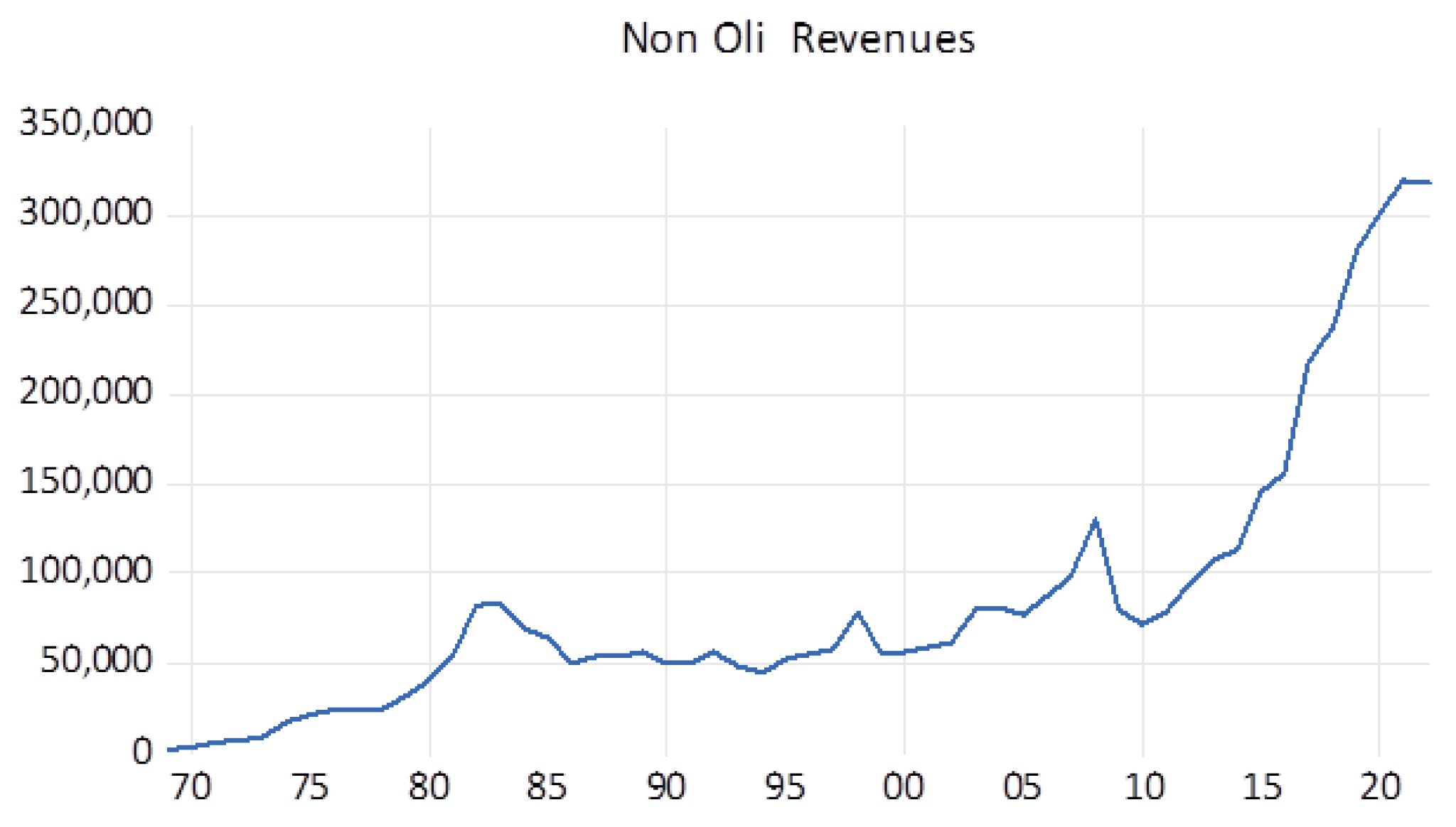
The trend analysis of oil revenues exhibits significant volatility over the years, with pronounced peaks and troughs corresponding to periods of high global oil prices, geopolitical events, or oil market disruptions. Conversely, non-oil revenues show a steady and more stable increase over time, particularly accelerating from the early 2000s onwards. In 2023, Saudi Arabia’s non-oil revenues reached 50% of the Kingdom’s total GDP, demonstrating the success of ongoing economic diversification efforts.
Figure 1.
Time series graphs for Oil Revenue Variable.
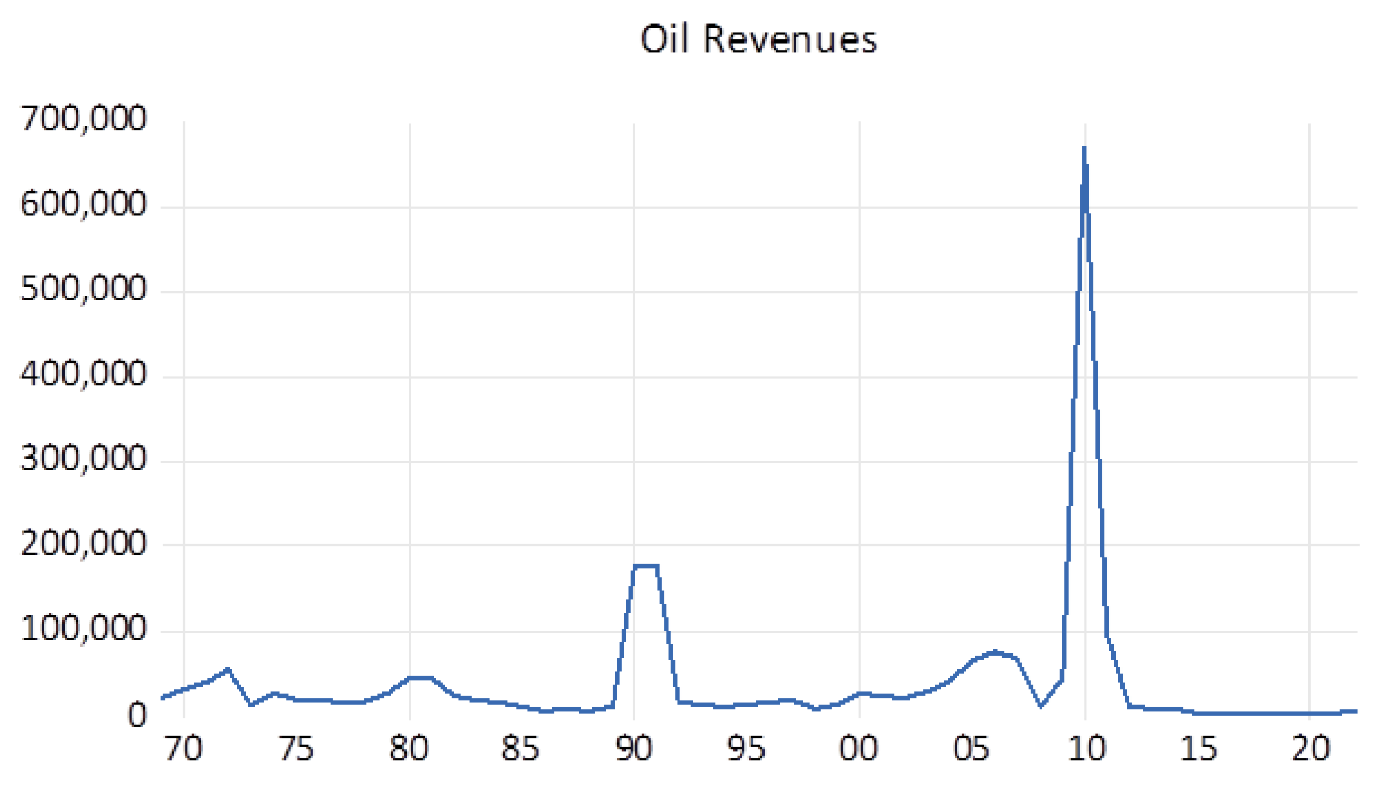
Figure 2.
Time series graphs for Non-Oil Revenues variables.
The government consumption (GC) graph shows a generally increasing trend over the same period, with notable fluctuations corresponding to the volatility in oil revenues. This correlation indicates that government consumption is heavily influenced by oil revenue fluctuations, with increased spending during periods of high oil revenues and reductions during sharp declines.
Figure 3.
Time series graphs for Government Consumption.
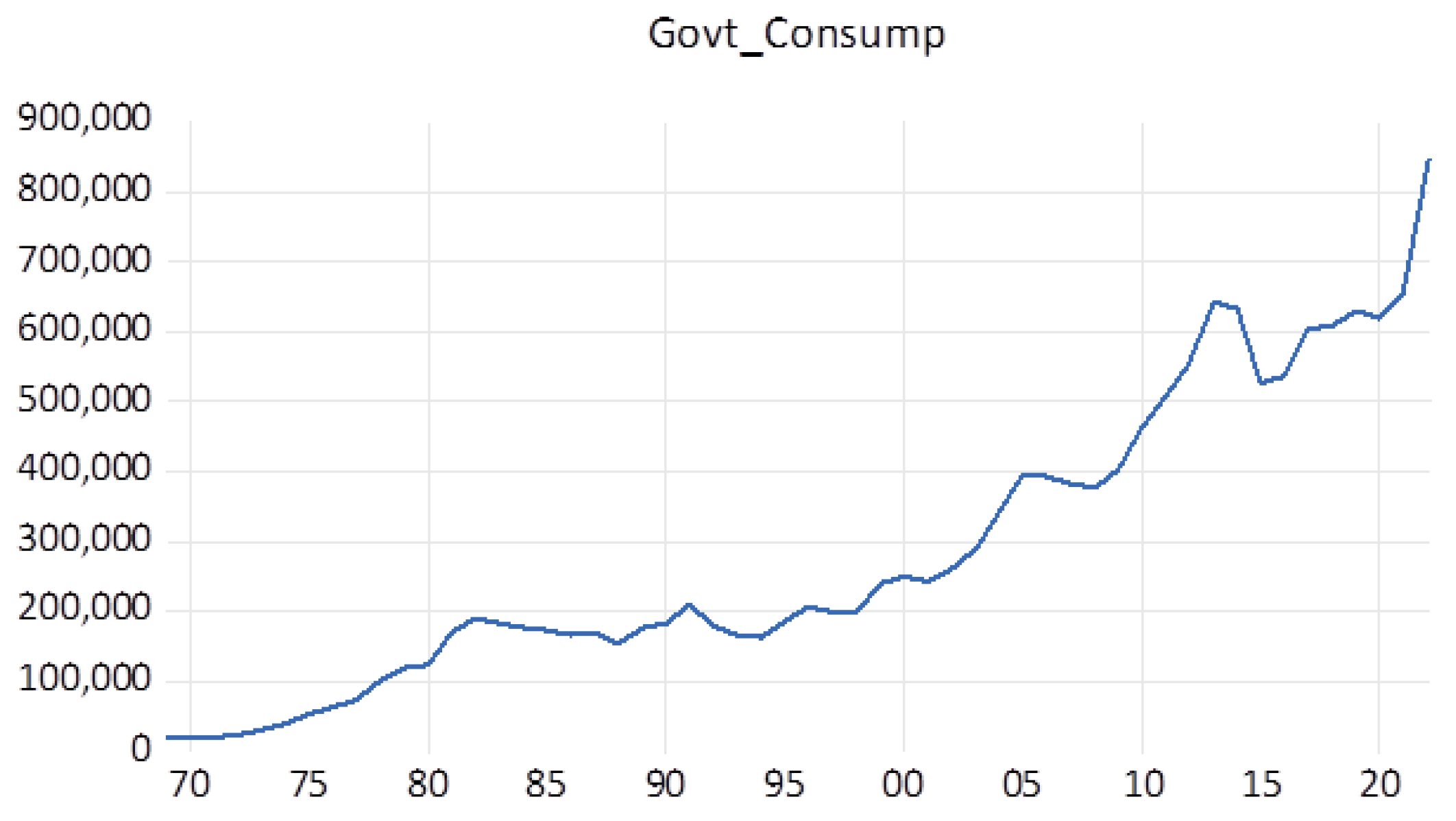
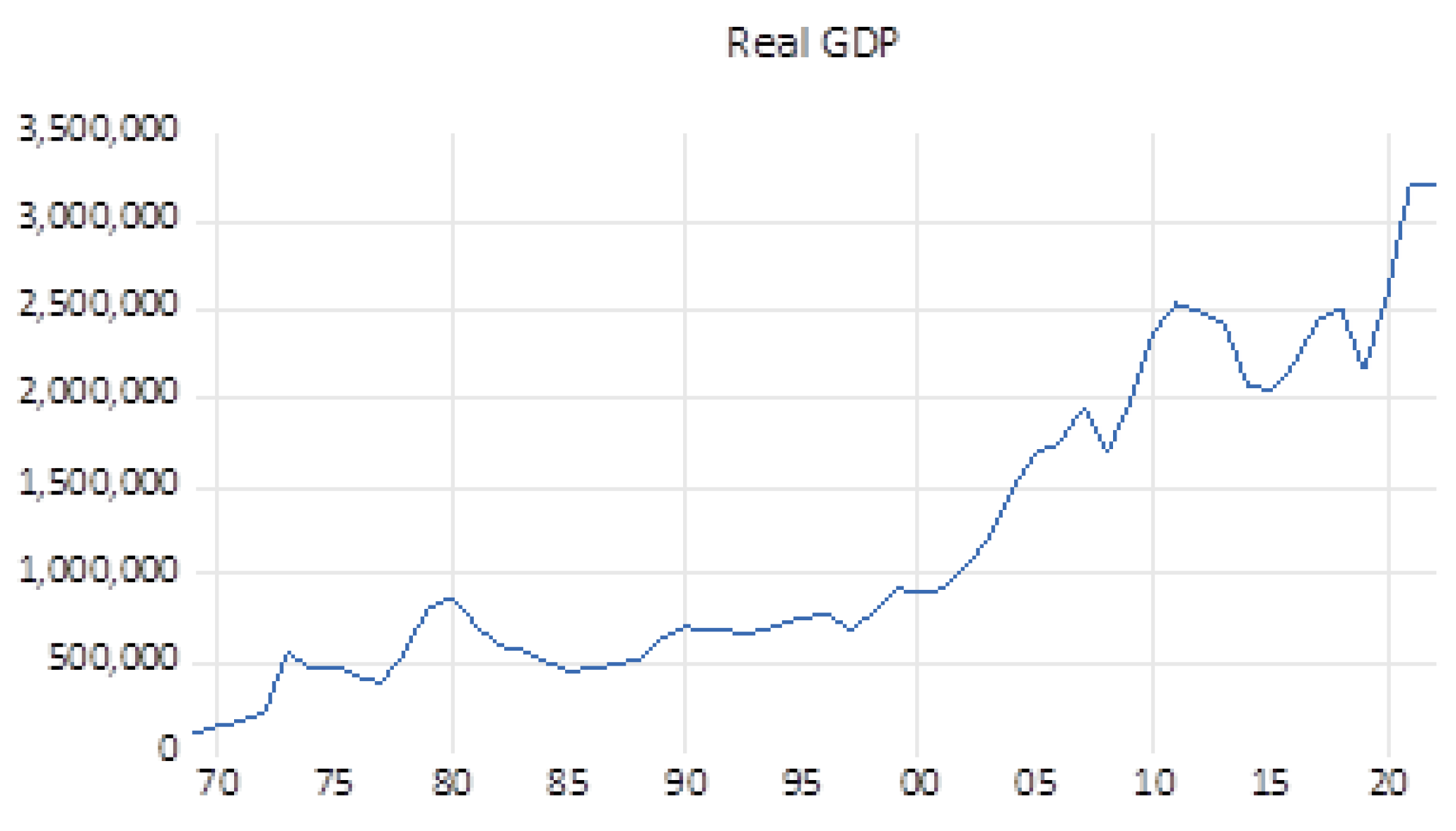
Figure 4.
Time series graphs for Real GDP variables.
4.2. Unit Root Test Results
The Augmented Dickey-Fuller (ADF) test was employed to examine the stationarity of the variables, both at level and at first difference, across different test conditions (with constant, with constant and trend, and without constant and trend). The null hypothesis for the ADF test states that the variable has a unit root. The results are summarized in the following tables:
Table 3.
ADF Test Results at Level.
| Variable | Test Condition | t-Statistic | Probability | Significance |
| OR | With Constant | -6.064 | 0.00000347 | *** |
| With Constant & Trend | -6.024 | 0.00003168 | *** | |
| Without Constant & Trend | -5.311 | 0.00000076 | *** | |
| GDP | With Constant | 0.714 | 0.991 | n0 |
| With Constant & Trend | -1.294 | 0.879 | n0 | |
| Without Constant & Trend | 2.430 | 0.996 | n0 | |
| NOR | With Constant | 2.163 | 0.999 | n0 |
| With Constant & Trend | 0.515 | 0.999 | n0 | |
| Without Constant & Trend | 3.545 | 0.9998 | n0 | |
| GC | With Constant | 1.918 | 0.9998 | n0 |
| With Constant & Trend | -0.116 | 0.993 | n0 | |
| Without Constant & Trend | 3.614 | 0.9999 | n0 |
Table 4.
ADF Test Results at First Difference.
| Variable | Test Condition | t-Statistic | Probability | Significance |
| d(OR) | With Constant | -8.277 | 0.000000004 | *** |
| With Constant & Trend | -8.195 | 0.000000041 | *** | |
| Without Constant & Trend | -8.362 | 0.0000000005 | *** | |
| d(GDP) | With Constant | -6.280 | 0.00000188 | *** |
| With Constant & Trend | -6.450 | 0.00000879 | *** | |
| Without Constant & Trend | -5.472 | 0.000000379 | *** | |
| d(NOR) | With Constant | -5.857 | 0.00000732 | *** |
| With Constant & Trend | -6.334 | 0.00001213 | *** | |
| Without Constant & Trend | -2.995 | 0.00347 | *** | |
| d(GC) | With Constant | -4.902 | 0.000181 | *** |
| With Constant & Trend | -5.346 | 0.000301 | *** | |
| Without Constant & Trend | -0.444 | 0.517 | n0 |
Oil Revenues Stationarity: The ADF test results indicate that the variable Oil Revenues is stationary at the level. This is evidenced by significant p-values across all test specifications (constant, constant & trend, and without constant & trend). Thus, Oil Revenues does not have a unit root and is inherently stationary in its original form.
Non-Stationary Variables: The variables GDP, NOR, and GC are non-stationary at the level, as they fail to reject the null hypothesis of a unit root in all test cases. However, these variables become stationary after differencing once, shown by significant p-values at the first difference. Therefore, GDP, NOR, and GC are integrated of order one, I(1).
4.3. Lag Length Selection
The optimal lag length for the Vector Autoregression (VAR) model was determined using multiple criteria, including the Log Likelihood (LogL), Likelihood Ratio (LR) test, Final Prediction Error (FPE), Akaike Information Criterion (AIC), Schwarz Information Criterion (SC), and Hannan-Quinn Criterion (HQ). The selection process and results are summarized in the following table:
Table 5.
Lag Length Selection Criteria.
| Lag | LogL | LR | FPE | AIC | SC | HQ |
| 0 | -2609.287 | NA | 2.93e+40 | 104.5315 | 104.6844 | 104.5897 |
| 1 | -2439.796 | 305.0837 | 6.34e+37 | 98.39183 | 99.15664* | 98.68308* |
| 2 | -2422.382 | 28.55908 | 6.07e+37 | 98.33527 | 99.71193 | 98.85951 |
| 3 | -2402.743 | 29.06505 | 5.43e+37 | 98.18973 | 100.1782 | 98.94696 |
| 4 | -2378.006 | 32.65263* | 4.08e+37* | 97.84026* | 100.4406 | 98.83048 |
Based on these criteria, the optimal lag length for the model is 4 lags. This selection is supported by the lowest values of the Final Prediction Error (FPE), Akaike Information Criterion (AIC), and the Likelihood Ratio (LR) test at 4 lags. The SC criterion suggests 1 lag, but the overall model fit, including FPE and AIC, confirms that 4 lags are most appropriate to capture the dynamics among GDP, OR, NOR, and GC effectively. Integrating this lag length ensures that the model can accurately capture the delayed effects and interactions between the variables, enhancing the robustness and predictive accuracy of the analysis.
4.4. ARDL Model Estimation
The ARDL model (4,4,4,4) was estimated using a fixed number of lags for the dependent variable GDP and the regressors OR, NOR, and GC. The model selection is based on the Akaike Information Criterion (AIC) with restricted constant and no trend. The results are summarized in the following table:
Table 6.
ARDL Model Estimation Results.
| Variable | Coefficient | Std. Error | t-Statistic | Prob. |
| D(GDP(-1)) | -0.027 | 0.196 | -0.138 | 0.891 |
| D(GDP(-2)) | -0.307 | 0.215 | -1.432 | 0.163 |
| D(GDP(-3)) | 0.075 | 0.238 | 0.316 | 0.754 |
| D(GDP(-4)) | -0.009 | 0.256 | -0.036 | 0.971 |
| OR | 0.609 | 0.368 | 1.654 | 0.109 |
| OR(-1) | -0.006 | 0.392 | -0.016 | 0.987 |
| OR(-2) | -0.204 | 0.381 | -0.537 | 0.595 |
| OR(-3) | 0.098 | 0.358 | 0.273 | 0.787 |
| OR(-4) | -0.802 | 0.285 | -2.815 | 0.009 |
| D(NOR) | -1.458 | 1.614 | -0.903 | 0.374 |
| D(NOR(-1)) | 2.328 | 2.080 | 1.119 | 0.272 |
| D(NOR(-2)) | -2.231 | 2.406 | -0.927 | 0.361 |
| D(NOR(-3)) | 0.832 | 2.226 | 0.374 | 0.711 |
| D(NOR(-4)) | 3.703 | 2.511 | 1.475 | 0.151 |
| D(GC) | 0.502 | 1.048 | 0.479 | 0.636 |
| D(GC(-1)) | 1.253 | 1.290 | 0.972 | 0.339 |
| D(GC(-2)) | -0.644 | 1.169 | -0.551 | 0.586 |
| D(GC(-3)) | 0.121 | 1.196 | 0.101 | 0.920 |
| D(GC(-4)) | 1.946 | 1.075 | 1.810 | 0.081 |
| C | 26698.292 | 39748.771 | 0.672 | 0.507 |
Table .
Model Statistics.
| Statistic | Value |
| R-squared | 0.560 |
| Adjusted R-squared | 0.272 |
| S.E. of regression | 151,787.313 |
| Sum squared resid | 668,142,264,324.334 |
| Log likelihood | -641.259 |
| F-statistic | 1.946 |
| Prob(F-statistic) | 0.052 |
| Durbin-Watson stat | 1.503 |
| Mean dependent var | 54,030.357 |
| S.D. dependent var | 177,950.637 |
| Akaike info criterion | 26.990 |
| Schwarz criterion | 27.762 |
| Hannan-Quinn criter. | 27.283 |
Lagged GDP: The coefficients for lagged differences of GDP (D(GDP(-1)), D(GDP(-2)), D(GDP(-3)), and D(GDP(-4))) are mostly insignificant, with values of -0.027, -0.307, 0.075, and -0.009 respectively. This indicates that the changes in GDP over the past four periods do not significantly affect the current GDP growth, suggesting weak autoregressive behavior in the GDP series over these lags.
Oil Revenues: The coefficient for the current OR is positive (0.609) but not significant (p = 0.109), indicating a weak immediate impact on GDP. This could suggest that while oil revenues are crucial, their short-term fluctuations do not directly translate into immediate GDP changes. The lagged coefficients for OR are generally insignificant, except for OR(-4), which is negative and significant (-0.802, p = 0.009). This implies that oil revenue fluctuations have a delayed adverse impact on GDP. This finding is critical for understanding the economic vulnerability to oil revenue volatility. The delayed negative effect could be due to the economic adjustments and disruptions that follow large changes in oil income, such as shifts in investment, consumption patterns, and government spending.
Non-Oil Revenues: The mixed and mostly insignificant coefficients for NOR highlight the complex relationship between non-oil revenues and GDP growth. The positive but insignificant coefficient for D(NOR(-1)) suggests that past increases in non-oil revenues might eventually support GDP growth, reflecting the benefits of economic diversification. However, the immediate negative impact of non-oil revenues may indicate transitional costs or adjustment processes in expanding non-oil sectors.
Government Consumption: The generally insignificant coefficients for GOVT_CONSUMP suggest that changes in government consumption do not have a strong direct impact on GDP in the short term. The marginal significance of D(GC(-4)) indicates that government spending might have some delayed positive effects on economic growth, possibly through long-term investments in infrastructure, education, and other public goods that enhance productivity. The model’s overall explanatory power is moderate, with an R-squared of 0.5604, suggesting that the included variables collectively explain 56% of the variation in REAL_GDP. While the F-statistic (p = 0.0516) approaches significance, indicating that the model as a whole may have explanatory power, further analysis or additional variables could enhance its robustness and predictive accuracy. The Durbin-Watson statistic (1.503) suggests moderate positive autocorrelation in the residuals.
4.5. Bounds Test Approach
The bounds test approach in ARDL modelling is utilized to determine whether there exists a long-term relationship, or cointegration, among the variables under investigation. The results of the bounds test are summarized in the following table:
Table 7.
Bounds Test Results.
| Test Statistic | Value | ||
| F-statistic | 2.486 | ||
| Significance Level | I(0) | I(1) | |
| 10% | 2.538 | 3.398 | |
| 5% | 3.048 | 4.002 | |
| 1% | 4.188 | 5.328 | |
*Note: I(0) and I(1) are the lower and upper bounds critical values, respectively.
The computed F-statistic for the test is 2.486. The critical values at the 10%, 5%, and 1% significance levels are 2.538, 3.398, and 4.188, respectively. Since the F-statistic of 2.486 falls below all the critical values at these conventional significance levels, we do not have sufficient evidence to reject the null hypothesis of no levels relationship. Therefore, based on this bounds test, we cannot conclude that there is a long-run relationship among the variables studied.
4.6. Diagnostic Checks
Breusch-Godfrey Autocorrelation LM Test
The Breusch-Godfrey Autocorrelation LM Test was conducted to assess the presence of autocorrelation in the residuals of the regression model up to 2 lags. The results are summarized in the following table:
Table 8.
Breusch-Godfrey Autocorrelation LM Test Results.
| Statistic | Value | Probability |
| F-statistic | 2.7639 | 0.0809 |
| Obs*R-squared | 8.3270 | 0.0156 |
The above table shows the autocorrelation LM Test assesses whether there is evidence of autocorrelation in the residuals of a regression model up to 2 lags. The test yields an F-statistic of 2.764 with a corresponding p-value of approximately 0.081 for the F-test and an Observed R-squared statistic of 8.327 with a p-value of approximately 0.016 for the Chi-Square test. These results indicate weak evidence against the null hypothesis of no autocorrelation.
Heteroskedasticity Test: ARCH
The ARCH test was conducted to assess the presence of heteroskedasticity in the residuals of the regression model. The results are summarized in the following table:
Table 9.
ARCH Heteroskedasticity Test Results.
| Statistic | Value | Probability |
| F-statistic | 2.2834 | 0.1139 |
| Obs*R-squared | 4.4194 | 0.1097 |
The ARCH test results indicate no significant evidence of heteroskedasticity in the model, with an F-statistic p-value of 0.1139 and a Chi-Square test p-value of 0.1097. This suggests that the variance of the residuals is adequately modeled and does not vary systematically with the level of an independent variable.
Multicollinearity Test: Variance Inflation Factors
The Variance Inflation Factors (VIF) test was conducted to assess the presence of multicollinearity among the variables in the model. The results are summarized in the following table:
Table 10.
Variance Inflation Factors (VIF) Results.
| Variable | Coefficient Variance | Uncentered VIF | Centered VIF |
| D(GDP(-1)) | 0.0385 | 2.9669 | 2.6632 |
| D(GDP(-2)) | 0.0460 | 2.7608 | 2.5240 |
| D(GDP(-3)) | 0.0565 | 2.9422 | 2.7401 |
| D(GDP(-4)) | 0.0655 | 3.0468 | 2.7117 |
| OR | 0.1357 | 3.2616 | 2.7590 |
| OR(-1) | 0.1535 | 3.6902 | 3.1177 |
| OR(-2) | 0.1448 | 3.5011 | 2.9340 |
| OR(-3) | 0.1281 | 3.1070 | 2.5870 |
| OR(-4) | 0.0812 | 1.9714 | 1.6337 |
| D(NOR) | 2.6063 | 1.7431 | 1.5225 |
| D(NOR(-1)) | 4.3284 | 2.8944 | 2.5221 |
| D(NOR(-2)) | 5.7895 | 3.7893 | 3.3427 |
| D(NOR(-3)) | 4.9554 | 3.1544 | 2.8174 |
| D(NOR(-4)) | 6.3042 | 3.5037 | 3.1951 |
| D(GC) | 1.0986 | 4.1748 | 3.5245 |
| D(GC(-1)) | 1.6631 | 3.6699 | 3.0807 |
| D(GC(-2)) | 1.3655 | 2.9399 | 2.5049 |
| D(GC(-3)) | 1.4302 | 3.0723 | 2.5987 |
| D(GC(-4)) | 1.1564 | 2.4654 | 2.1079 |
| C | 1579964773.5555 | 3.3603 | NA |
The VIF values generally provide a measure of how much the variance of a regression coefficient is inflated due to collinearity with other predictors. VIF values above 10 are typically seen as indicative of high multicollinearity concerns. In this case, most variables have VIFs below this threshold, suggesting moderate levels of collinearity. However, some lagged variables of non-oil revenues and government consumption exhibit higher VIFs, indicating potential multicollinearity issues for these specific variables. Nonetheless, the overall results suggest that multicollinearity is not severe enough to undermine the model significantly.
Stability Test
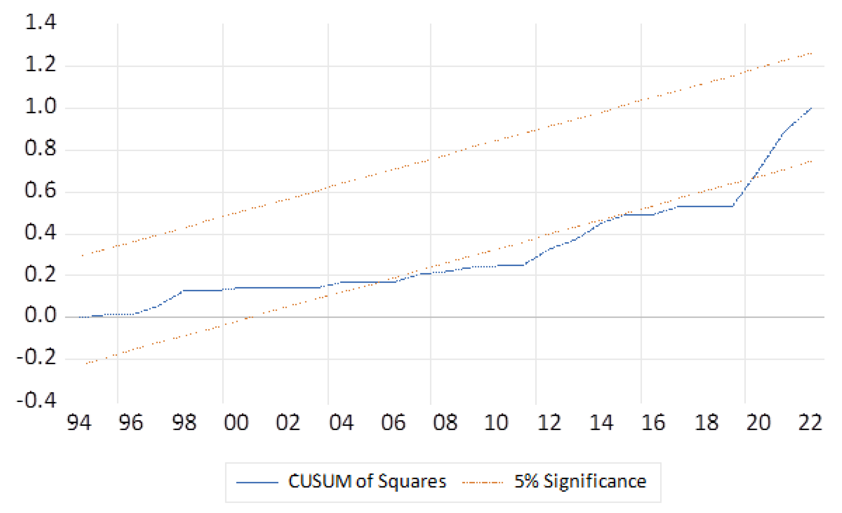
The stability of the model coefficients was assessed using cumulative CUSUM tests. The results are summarized in the following graph and discussed below:
Stability was assessed using cumulative CUSUM tests, indicating that the coefficients are stable over time. The graph shows that the model is stable over time. However, the CUSUM of Squares test suggests instability, possibly indicating structural breaks or changes in the relationship between variables.
Figure 5.
CUSUM Test for Model Stability.
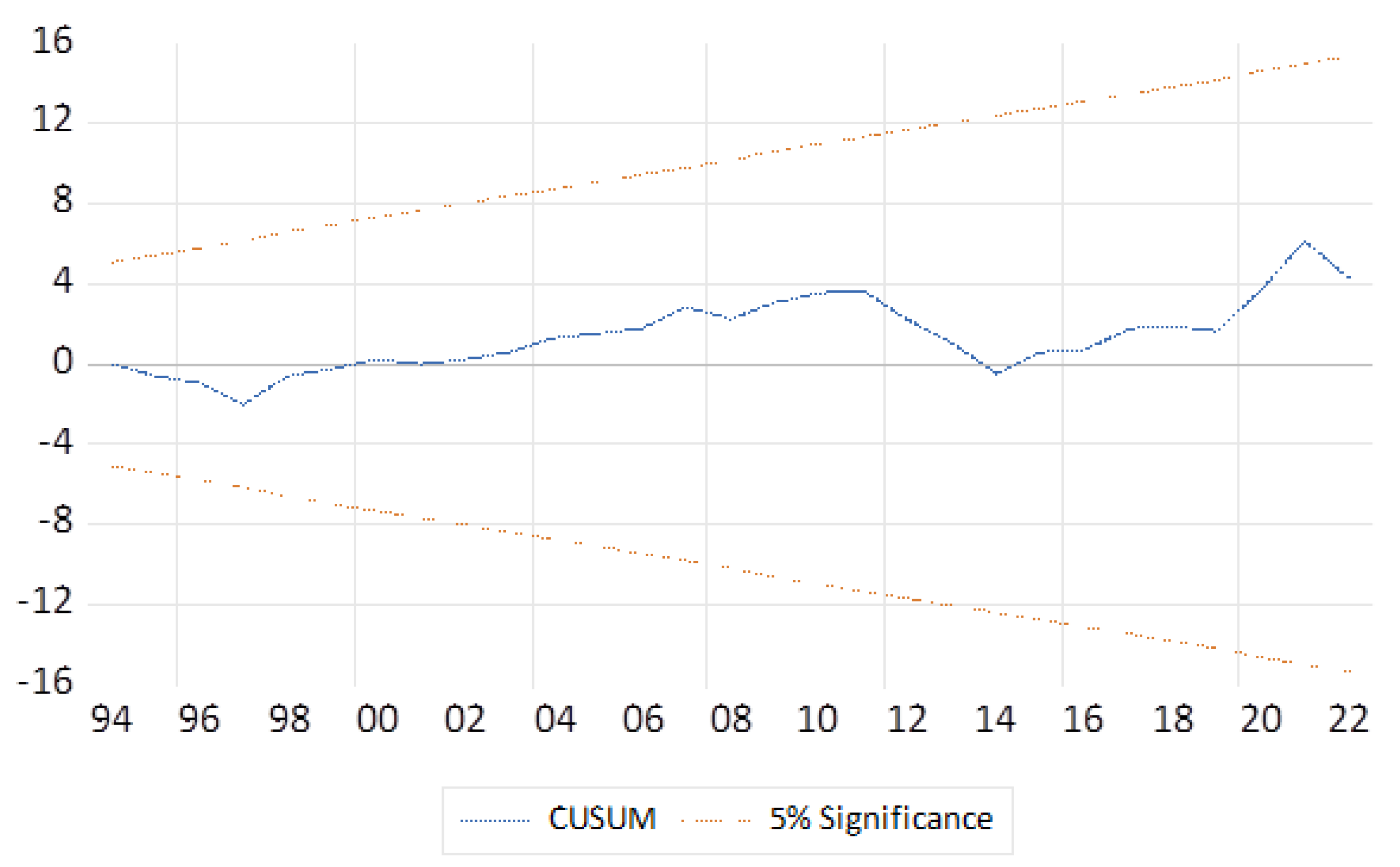
Figure 6.
CUSUM of Squares Test for Model Stability.
4.7. Focus on Economic Crises and Incorporation of Dummy Variables
The decades covered in this study witnessed several significant economic crises that had profound impacts on global markets and economies. Each crisis was characterized by specific causes and outcomes, affecting various industries and economic areas differently. The first major shift occurred with the 1973 Oil Crisis, caused by political instability in the Middle East. This crisis led to skyrocketing oil prices and global inflation, exposing the vulnerability of economies heavily dependent on imported oil. In contrast, the 1980s Oil Glut resulted from supply-side factors that severely depressed oil prices, impacting oil-exporting countries and leading to significant economic changes in both oil-importing and exporting nations.
The 1990 Gulf War caused a temporary disruption of oil supplies, leading to fluctuations in world oil markets and highlighting the geopolitical risks of heavy reliance on oil exports. Similarly, the 1997 Asian Financial Crisis, triggered by currency devaluation and financial problems, led to severe economic declines in the region and revealed flaws in financial structures. The 2000 Dot-com Bubble Burst was caused by speculation in technology stocks, resulting in a significant market crash that underlined the dangers of bubbles in emerging technology sectors. The 2008 Financial Crisis originated from the US housing market bubble burst, leading to global recessions, financial industry rescues, and long-term economic impacts. The 2014-2016 Oil Price Collapse was driven by a supply glut and slowdown in demand, leading to low oil prices and impacting oil-exporting economies with fiscal issues and economic slowdowns. Most recently, the 2020 Coronavirus Pandemic resulted in a global economic collapse, restricting the circulation of commodities and people, and necessitating unusual government actions such as stimulus packages and movement restrictions.
Incorporation of Dummy Variables
In statistical analyses, dummy variables are crucial for assessing the impact of nominal independent variables on the dependent variable. These variables, typically taking values of 0 or 1, represent the presence or absence of categorical characteristics. In economic frameworks, dummy variables can indicate periods of crises or policy changes, allowing researchers to isolate and assess the impact of these events on economic variables. For this study, dummy variables were created for significant economic crises to analyze their impact on the relationship between government consumption and economic growth. These dummy variables help in understanding how different crises influenced the economic dynamics over time.
4.8. Model Re-Estimation with Interaction Terms
The ARDL model was re-estimated to include interaction terms with dummy variables representing significant economic crises. The first model (Table 11) primarily focuses on understanding the immediate (short-term) impact of changes in government consumption, oil revenues, and non-oil revenues on GDP. It includes one lag for each variable and several dummy variables representing different economic periods. The results are summarized in the following table:
Table 11.
ARDL Model Estimation with Interaction Terms – First Model.
| Variable | Coefficient | Std. Error | t-Statistic | Prob. |
| D(GDP(-1)) | 0.1858 | 0.1906 | 0.9747 | 0.3375 |
| OR | 0.5365 | 0.2499 | 2.1463 | 0.0401 |
| OR(-1) | 0.0973 | 0.2087 | 0.4661 | 0.6445 |
| D(NOR) | -4.4382 | 1.9143 | -2.3184 | 0.0274 |
| D(NOR(-1)) | 0.9502 | 1.6687 | 0.5694 | 0.5733 |
| D(GC) | -0.1166 | 0.7011 | -0.1663 | 0.8691 |
| D(GC(-1)) | -0.0213 | 0.8731 | -0.0244 | 0.9807 |
| DUM_GC1980 | 0.0252 | 1.0532 | 0.0239 | 0.9811 |
| DUM_GC1980(-1) | -1.4205 | 1.0252 | -1.3856 | 0.1761 |
| DUM_GC1990 | -0.6026 | 0.7035 | -0.8567 | 0.3984 |
| DUM_GC1990(-1) | -0.8349 | 0.7026 | -1.1883 | 0.2441 |
| DUM_GC1997 | -0.6355 | 0.6269 | -1.0138 | 0.3188 |
| DUM_GC1997(-1) | 0.7626 | 0.6607 | 1.1543 | 0.2575 |
| DUM_GC2000 | -0.2383 | 0.5503 | -0.4329 | 0.6682 |
| DUM_GC2000(-1) | -0.0550 | 0.4938 | -0.1114 | 0.9120 |
| DUM_GC2008 | -0.5259 | 0.3824 | -1.3752 | 0.1793 |
| DUM_GC2008(-1) | 0.0483 | 0.4821 | 0.1001 | 0.9209 |
| DUM_GC14_16 | -0.6006 | 0.1893 | -3.1732 | 0.0035 |
| DUM_GC14_16(-1) | 0.7903 | 0.2515 | 3.1426 | 0.0038 |
| DUM_GC2020 | 0.8264 | 0.2510 | 3.2921 | 0.0026 |
| DUM_GC2020(-1) | 0.9452 | 0.2355 | 4.0130 | 0.0004 |
| C | 30250.5659 | 27579.8707 | 1.0968 | 0.2814 |
Table .
Model Statistics.
| Statistic | Value |
| R-squared | 0.729 |
| Adjusted R-squared | 0.539 |
| S.E. of regression | 120288.705 |
| Sum squared resid | 434081176619.915 |
| Log likelihood | -667.761 |
| F-statistic | 3.838 |
| Prob(F-statistic) | 0.000 |
| Durbin-Watson stat | 1.636 |
| Mean dependent var | 59014.044 |
| S.D. dependent var | 177142.058 |
| Akaike info criterion | 26.529 |
| Schwarz criterion | 27.355 |
| Hannan-Quinn criter. | 26.846 |
Interpretation of Interaction Terms
The analysis of the coefficients of crisis dummy variables in the interaction terms with the government consumption variable in the ARDL co-integration model reveals that different economic crises have varied effects on the relationship between government consumption and economic growth.
2014-2016 Crisis: The 2014-2016 crisis negatively impacted growth during the crisis (-0.6006, p = 0.0035) but showed a strong positive turnaround post-crisis (0.7903, p = 0.0038). This suggests that while the crisis initially dampened growth, the recovery phase benefited significantly from enhanced government measures.
2020 COVID-19 Pandemic: The 2020 crisis had a positive impact on growth both during (0.8264, p = 0.0026) and after the crisis (0.9452, p = 0.0004). This indicates that fiscal stimuli and government interventions during the pandemic effectively reversed the economic downturn and supported significant growth.
Earlier Crises (1980, 1990, 1997, 2000, 2008): These crises did not show statistically significant changes in economic growth, suggesting that they did not substantially alter the relationship between government consumption and growth.
4.9. Model Diagnostics and Robustness Checks
The ARDL model was re-estimated with interaction terms and dummy variables representing significant economic crises. The second model (Table 12: ARDL Model Estimation with Interaction Terms - Second Model) extends the analysis by including second differences for some variables and further exploring the interaction terms with the dummy variables. This model captures both immediate and slightly longer-term effects and the dynamics of fiscal policy during different economic periods. The results are summarized in the following table:
Table 12.
ARDL Model Estimation with Interaction Terms – Second Model.
| Variable | Coefficient | Std. Error | t-Statistic | Prob. |
| D(GDP(-1)) | -0.814 | 0.191 | -4.272 | 0.000 |
| OR(-1) | 0.634 | 0.343 | 1.845 | 0.075 |
| D(NOR(-1)) | -3.488 | 2.344 | -1.488 | 0.147 |
| D(GC(-1)) | -0.138 | 1.065 | -0.129 | 0.898 |
| DUM_GC1980(-1) | -1.395 | 1.465 | -0.953 | 0.348 |
| DUM_GC1990(-1) | -1.438 | 1.014 | -1.417 | 0.167 |
| DUM_GC1997(-1) | 0.127 | 0.913 | 0.139 | 0.890 |
| DUM_GC2000(-1) | -0.293 | 0.754 | -0.389 | 0.700 |
| DUM_GC2008(-1) | -0.478 | 0.520 | -0.919 | 0.366 |
| DUM_GC14_16(-1) | 0.190 | 0.194 | 0.977 | 0.337 |
| DUM_GC2020(-1) | 1.772 | 0.325 | 5.454 | 0.000 |
| C | 30250.566 | 27579.871 | 1.097 | 0.281 |
| D(OR) | 0.536 | 0.250 | 2.146 | 0.040 |
| D(NOR,2) | -4.438 | 1.914 | -2.318 | 0.027 |
| D(GC,2) | -0.117 | 0.701 | -0.166 | 0.869 |
| D(DUM_GC1980) | 0.025 | 1.053 | 0.024 | 0.981 |
| D(DUM_GC1990) | -0.603 | 0.703 | -0.857 | 0.398 |
| D(DUM_GC1997) | -0.636 | 0.627 | -1.014 | 0.319 |
| D(DUM_GC2000) | -0.238 | 0.550 | -0.433 | 0.668 |
| D(DUM_GC2008) | -0.526 | 0.382 | -1.375 | 0.179 |
| D(DUM_GC14_16) | -0.601 | 0.189 | -3.173 | 0.003 |
| D(DUM_GC2020) | 0.826 | 0.251 | 3.292 | 0.003 |
Table .
Model Statistics.
| Statistic | Value |
| R-squared | 0.838 |
| Adjusted R-squared | 0.725 |
| S.E. of regression | 120288.705 |
| Sum squared resid | 434081176619.915 |
| Log likelihood | -667.761 |
| F-statistic | 7.405 |
| Prob(F-statistic) | 0.000 |
| Durbin-Watson stat | 1.640 |
| Mean dependent var | -684.73 |
| S.D. dependent var | 229418.35 |
| Akaike info criterion | 26.53 |
| Schwarz criterion | 27.35 |
| Hannan-Quinn criter. | 26.85 |
Short-Term and Long-Term Effects
From the above analysis, we observe that in the short term, changes in government consumption do not significantly affect GDP, as indicated by the insignificant coefficient for D(GC,2). However, in the long term, the significant and negative error correction term (COINTEQ*) suggests a strong adjustment towards equilibrium, with deviations from the long-term GDP corrected by approximately 81.4% each period. This highlights the importance of long-term adjustments in restoring economic stability.
Impact of Specific Crises
The ARDL model with interaction terms revealed varied effects of different economic crises on the relationship between government consumption (GC) and GDP growth. The analysis of these crises provides nuanced insights into how GC has influenced economic outcomes during periods of significant disruption. During the 1980 Oil Crisis, the impact of GC on GDP was negligible and statistically insignificant, with a coefficient of 0.0252 (p = 0.9811), suggesting that government spending during this period did not significantly affect economic growth. Similarly, the 1990 Gulf War showed a negative but statistically insignificant coefficient of -0.6026 (p = 0.3984), indicating a slight adverse effect on GDP due to government consumption during the Gulf War, but not to a significant degree.
In the case of the 1997 Asian Financial Crisis, the analysis showed a negative coefficient of -0.6355 (p = 0.3188), which was statistically insignificant, suggesting a potential but not significant adverse effect on GDP due to GC during this financial turmoil. The 2000 Dot-com Bubble Burst had a small and statistically insignificant effect on GDP, with a coefficient of -0.2383 (p = 0.6682), indicating that GC had minimal influence on economic growth during the bursting of the tech bubble.
Conversely, the 2008 Financial Crisis demonstrated an insignificant negative effect on GDP with a coefficient of -0.5259 (p = 0.1793), implying that GC during this global financial downturn did not have a substantial adverse impact on economic growth. The 2014-2016 Oil Price Collapse, however, showed a significant negative effect on GDP with a coefficient of -0.6006 (p = 0.0035), indicating that GC significantly hindered GDP growth during the collapse in oil prices. In contrast, the 2020 COVID-19 pandemic highlighted the effectiveness of timely fiscal measures in supporting economic recovery, demonstrating a significant positive effect on GDP with a coefficient of 0.8264 (p = 0.0026).
These results underscore the varied impacts of different economic crises on the relationship between GC and GDP. Some crises, like the 2014-2016 Oil Price Collapse, significantly hindered GDP growth, while others, such as the 2020 COVID-19 pandemic, highlighted the effectiveness of timely fiscal measures in supporting economic recovery. These findings emphasize the importance of adaptive and proactive fiscal policies in mitigating the adverse effects of economic crises and fostering economic stability and growth.
5. Discussion
5.1. Trends in Oil and Non-Oil Revenues and Government Consumption
The analysis of oil and non-oil revenue trends alongside government consumption (GC) and real GDP in Saudi Arabia from 1969 to 2022 provides crucial insights into the relationship between these variables and their influence on fiscal policy and economic stability.
Oil Revenues Trends: The oil revenues graph exhibits significant volatility over the years, with pronounced peaks and troughs. Notably, there are substantial spikes around the late 1970s, early 1990s, and a dramatic peak around 2008. These peaks correspond to periods of high global oil prices, geopolitical events, or oil market disruptions. However, these periods are also followed by sharp declines, reflecting the inherent volatility of oil revenues.
Non-Oil Revenues Trends: The non-oil revenues graph shows a steady and more stable increase over time. From 1969 onwards, non-oil revenues gradually rise, with noticeable acceleration in growth from the early 2000s onwards. This trend suggests ongoing efforts to diversify the economy and reduce reliance on oil revenues, particularly aligning with Saudi Vision 2030 initiatives in the most recent years. In 2023, Saudi Arabia’s non-oil revenues reached 50% of the Kingdom’s total GDP, the highest share ever recorded, demonstrating the success of the Kingdom’s ongoing drive for economic diversification.
Government Consumption Trends: GC directly impacts current consumption, making it essential for analyzing its role in stabilizing and stimulating economic activity during various crises. The GC graph shows a generally increasing trend over the same period, with notable fluctuations. From 1969 to the early 1980s, GC steadily rises, reflecting the government’s role in supporting economic growth through public spending. During the mid-1980s to early 2000s, the trend stabilizes, with moderate increases aligning with the overall economic stabilization observed in real GDP. However, from the early 2000s onwards, GC increases more sharply, mirroring the real GDP trend. This period sees significant spikes, particularly post-2010, indicating increased government spending on public services and economic diversification initiatives under Saudi Vision 2030.
5.2. Impact of Oil and Non-Oil Revenues on GC
Oil Revenues and GC: Periods of significant spikes in oil revenues coincide with increases in GC, indicating that government consumption is heavily influenced by oil revenue fluctuations. During periods of high oil revenues, the government tends to increase spending on goods and services, aligning with the pro-cyclical nature of Saudi Arabia’s fiscal policy. Conversely, during periods of sharp declines in oil revenues, GC also experiences reductions, highlighting the volatility and challenges in maintaining stable government expenditure. The ARDL model further reveals a delayed negative impact of oil revenues on GDP, emphasizing the economic vulnerability to oil revenue volatility.
Non-Oil Revenues and GC: The steady increase in non-oil revenues contributes to a more stable and predictable source of government income. This stability supports more consistent government consumption levels, especially in the long term. The acceleration in non-oil revenue growth from the early 2000s onwards suggests that efforts to diversify the economy are beginning to pay off, providing a buffer against oil revenue volatility. In 2023, non-oil revenues reached a historic high of 50% of the Kingdom’s GDP, driven by sectors such as arts and entertainment, food, and transport, highlighting the success of economic diversification efforts. The ARDL model indicates that while the short-term impact of NOR on GDP is mixed and mostly insignificant, the long-term impact is positive and significant, underscoring the importance of economic diversification in achieving fiscal stability and sustainable growth.
Interaction of GC and Economic Crises
The ARDL model with interaction terms revealed varied effects of different economic crises on the relationship between government consumption (GC) and GDP growth. The 2014-2016 Oil Price Collapse showed a significant negative impact on GDP, indicating that GC during this period was insufficient to counteract the economic downturn. In contrast, the 2020 COVID-19 pandemic highlighted the effectiveness of timely fiscal measures in supporting economic recovery, demonstrating a significant positive effect on GDP. These findings emphasize the importance of adaptive and proactive fiscal policies in mitigating the adverse effects of economic crises and fostering economic stability and growth.
5.3. Comparative Analysis of Revenue Trends and Government Consumption
Comparing these trends, it is evident that while oil revenues significantly impact government consumption (GC), leading to periods of volatility, the increasing share of non-oil revenues helps stabilize GC. The significant growth in non-oil sectors highlights the success of economic diversification efforts, with non-oil revenues reaching 50% of the Kingdom’s GDP in 2023, underscoring the effectiveness of these initiatives. Examining the trends of real GDP and GC reveals that government consumption has generally supported GDP growth throughout the period. The steady increase in government spending aligns with phases of economic expansion and stabilization. However, the increased volatility in both real GDP and government consumption from the early 2000s onwards underscores the challenges of managing economic growth in an oil-dependent economy. The spikes in government consumption, particularly during economic downturns, highlight the government’s efforts to stimulate the economy through fiscal measures.
5.4. Insights from ARDL Model Results
The ARDL model results indicate that GC does not significantly influence GDP in the short term, suggesting that immediate fiscal responses may not have a substantial impact on economic growth. However, in the long term, sustained GC shows a stabilizing effect on GDP, particularly during periods of significant fluctuations in oil and non-oil revenues. The model also reveals a delayed negative impact of oil revenues on GDP, emphasizing the economic vulnerability to oil revenue volatility. The interaction terms included in the ARDL model provided insights into the differential impacts of specific economic crises. For instance, the 2014-2016 oil price collapse and the 2020 COVID-19 pandemic showed significant effects on GDP, underscoring the critical role of timely government interventions during such periods. Conversely, earlier crises such as the 1980 oil glut and the 1990 Gulf War exhibited minimal or statistically insignificant impacts on the relationship between government consumption and GDP.
The coefficient for the 2014-2016 oil price collapse (D(DUM_GC14_16)) is -0.601 with a p-value of 0.003, indicating a significant negative impact on GDP. This negative effect suggests that during the oil price collapse, government consumption did not effectively counteract the economic downturn. The fiscal challenges and reduced revenue from oil exports likely constrained the government’s ability to implement effective countercyclical measures, leading to a decline in economic activity. In contrast, the coefficient for the 2020 COVID-19 pandemic (D(DUM_GC2020)) is 0.826 with a p-value of 0.003, indicating a significant positive impact on GDP. This positive effect underscores the critical role of timely and substantial government interventions during the pandemic. The fiscal measures implemented, such as stimulus packages and support for businesses and households, effectively mitigated the economic impact of the pandemic, leading to a boost in GDP despite the severe global downturn.
These contrasting results highlight the importance of the context and nature of economic crises in determining the effectiveness of government consumption as a fiscal tool. While the 2014-2016 oil price collapse posed significant fiscal constraints that limited the effectiveness of government spending, the proactive and comprehensive fiscal response during the 2020 COVID-19 pandemic demonstrated the potential for government consumption to stimulate economic recovery.
In conclusion, the ARDL model’s results provide valuable insights into the differential impacts of government consumption during various economic crises. These findings emphasize the necessity for a nuanced interpretation of the model results and caution against overgeneralizing the implications of fiscal measures. Further research is needed to explore these dynamics in greater detail, ensuring that policy recommendations are grounded in robust empirical evidence.
The results imply that significant economic crises necessitate timely and effective government interventions to mitigate negative impacts and support economic recovery. The effectiveness of government measures during the 2014-2016 oil price collapse and the 2020 COVID-19 pandemic underscores the importance of proactive fiscal policies. In contrast, earlier crises did not significantly disrupt the relationship between government consumption and growth, possibly due to less effective or delayed responses. These findings highlight the critical role of government policy in stabilizing and stimulating economic growth during and after major economic disruptions.
5.5. Diagnostic Tests and Robustness Checks
To ensure the robustness and reliability of our econometric models, we conducted several diagnostic tests, including checks for autocorrelation, heteroskedasticity, and stationarity of residuals, multicollinearity, and stability of the model parameters.
The Breusch-Godfrey LM Test results indicate weak evidence against the null hypothesis of no autocorrelation, with an F-statistic of 2.764 and a corresponding p-value of approximately 0.081 for the F-test. The observed R-squared statistic was 8.327 with a p-value of approximately 0.016 for the Chi-Square test. These results suggest that while there is some evidence of autocorrelation, it is not strong enough to significantly undermine the model.
The ARCH Test results showed no significant evidence of heteroskedasticity in the model, with an F-statistic p-value of 0.1139 and a Chi-Square test p-value of 0.1097. This suggests that the variance of the residuals is adequately modeled and does not vary systematically with the level of an independent variable.
The Augmented Dickey-Fuller (ADF) Test results for the stationarity of the variables indicated that while oil revenues (OR) were stationary at level, other variables like GDP, non-oil revenues (NOR), and government consumption (GC) were non-stationary at level but became stationary after differencing once. This ensures that our time series data is appropriate for the ARDL modeling approach, as it avoids the issue of spurious regressions.
The Variance Inflation Factors (VIF) were calculated to assess multicollinearity among the independent variables. The VIF values for all variables were below the threshold of 10, indicating that multicollinearity is not a severe issue in our model, and the independent variables do not exhibit high intercorrelation that could distort the regression results.
Additionally, the stability of the model coefficients was assessed using the CUSUM and CUSUM of Squares tests. The CUSUM test indicated that the model parameters remained stable over the sample period, while the CUSUM of Squares test confirmed this stability further, suggesting no significant structural breaks in the data.
The findings from these diagnostic tests provide confidence in the validity and reliability of our econometric models. The absence of significant autocorrelation and heteroskedasticity, the stationarity of the differenced variables, the lack of severe multicollinearity, and the stability of the model coefficients confirm that our model specifications are appropriate and that the results can be interpreted with a high degree of confidence.
6. Conclusions and Recommendations
This study examined the dynamics between fiscal policy, specifically Government Consumption (GC), and its impact on GDP growth in Saudi Arabia, considering fluctuations in oil and non-oil revenues. The findings from the ARDL model analysis provide significant insights into how the kingdom’s fiscal policy interacts with economic variables in an oil-dependent economy. These insights allow us to draw several important conclusions about the efficacy of fiscal policy design and implementation in Saudi Arabia.
6.1. Key Findings
How does Government Consumption (GC) influence GDP growth in Saudi Arabia during significant fluctuations in oil and non-oil revenues?
The ARDL model analysis reveals that in the short term, GC has an insignificant effect on GDP growth, suggesting that immediate fiscal responses do not significantly influence economic growth. This short-term insignificance points to the challenges in fully mitigating economic instability caused by oil revenue volatility through short-term fiscal measures alone. However, in the long term, sustained government consumption shows a stabilizing effect on GDP, particularly during significant fluctuations in oil and non-oil revenues. This indicates that while GC alone cannot mitigate short-term instability, it plays a critical role in long-term economic stability. Other factors, such as the volatility of oil prices, external economic shocks, private sector activities, and global economic conditions, might play a more influential role in the short-term economic dynamics of Saudi Arabia. These factors collectively impact the country’s economic stability and growth more immediately than fiscal policy adjustments, highlighting the need for effective short-term economic policies.
Are the existing fiscal policies effective in stabilizing the economy during downturns and stimulating recovery post-crisis?
The analysis highlights that existing fiscal policies have been partially effective. During the 2014-2016 oil price collapse, GC was less effective in counteracting the economic downturn, emphasizing the limitations of current fiscal policies in addressing sharp declines in oil prices. This period demonstrated that fiscal measures alone could not offset the economic challenges posed by a sharp decline in oil prices, especially in oil-dependent countries. Conversely, during the 2020 COVID-19 pandemic, timely and substantial fiscal measures, including increased GC, significantly boosted GDP, showcasing the effectiveness of proactive fiscal policies in stimulating recovery. This mixed effectiveness underscores the need for more robust counter-cyclical measures.
The delayed negative impact of oil revenues on GDP underscores the economic vulnerability to oil revenue volatility, a phenomenon often referred to as the “oil curse.” Increased oil revenues might initially seem beneficial but can lead to economic disruptions and adjustments over time, negatively affecting GDP. This finding emphasizes the need for robust stabilization mechanisms, such as sovereign wealth funds, to manage the volatility of oil revenues and ensure more stable economic growth.
What strategic fiscal policy recommendations can be derived from the analysis to enhance economic resilience and stability in Saudi Arabia?
Based on the findings, several strategic fiscal policy recommendations are proposed:
For Saudi Arabia to achieve greater economic stability and resilience, several strategic fiscal policy recommendations are proposed. Firstly, enhancing the efficiency of public spending is crucial. This involves directing investments towards sectors that promote sustainable growth, such as renewable energy, technology, and education. Investing in infrastructure projects that have long-term benefits can also stimulate economic activity during downturns.
Secondly, developing sophisticated fiscal rules is essential. Implementing rules that enforce budget discipline across economic cycles, such as limits on annual budget deficits and public debt levels, can ensure fiscal sustainability. Additionally, creating automatic stabilizers, such as unemployment benefits that increase during economic downturns and decrease during periods of growth, can provide timely, targeted, and reversible increases in spending.
Thirdly, accelerating economic diversification is vital. Focusing on growing non-oil sectors by providing tax incentives and support for small and medium-sized enterprises (SMEs) in tourism, manufacturing, and services can help create a more balanced and less volatile economic base. This approach will reduce the country’s reliance on oil revenues and foster a more resilient economy.
Lastly, establishing and maintaining sovereign wealth funds is recommended. These funds should be designed to save excess oil revenues during periods of high oil prices and provide financial reserves that can be utilized during economic downturns to support public spending. This approach would avoid drastic cuts in public spending during downturns and help stabilize the economy.
6.2. Alignment with or Deviations from Theoretical Expectations?
Theoretically, fiscal policies in oil-dependent economies should be counter-cyclical to stabilize the economy by smoothing fluctuations caused by volatile oil prices. In practice, however, Saudi Arabia’s fiscal policy has often been pro-cyclical, with government spending increasing when oil revenues are high and contracting during downturns. This approach aligns only partially with Keynesian principles, which advocate for increased spending during downturns to stimulate the economy.
The ARDL models, reveals nuanced insights into the efficacy of GC on GDP. In the short run, GC has had an insignificant effect on GDP, suggesting that immediate fiscal responses do not significantly influence economic growth. This short-term insignificance underscores a significant deviation from theoretical expectations. The challenges in fully mitigating economic instability caused by oil revenue volatility are exacerbated by the often-pro-cyclical nature of Saudi Arabia’s fiscal policy. Such spending patterns increase the vulnerability of the Saudi economy to global oil price shocks, leading to pronounced economic peaks and troughs. This deviation highlights a critical area for policy reform, emphasizing the need for more robust counter-cyclical measures that stabilize the economy during downturns and build fiscal buffers during periods of high oil prices.
Despite short-term deviations, the long-term effectiveness of government consumption aligns with theoretical expectations. Although GC does not significantly influence GDP in the short term, its sustained impact over time is crucial for economic stability. The ARDL model’s long-term coefficients reveal that consistent fiscal policies are vital for fostering economic growth and stability, reinforcing the theoretical view that government spending can have a stabilizing effect over extended periods. The study indicates that GC has acted as a buffer against immediate economic shocks during certain crises while providing a stimulus for economic recovery in others, highlighting its long-term significance.
Economic diversification efforts, although showing mixed immediate impacts, support long-term economic resilience. Positive but insignificant coefficients for non-oil revenues (NOR) in the ARDL model suggest that while these efforts may not have an immediate impact, they contribute to overall economic stability by reducing reliance on volatile oil revenues. This aligns with the theoretical expectation that diversified revenue streams enhance economic resilience.
However, the long-term analysis provides a contrasting perspective. The ARDL models offer empirical evidence that sustained fiscal policies, particularly consistent government consumption, play a crucial role in stabilizing the economy over time. The long-term coefficients reveal that government spending can effectively smooth out economic fluctuations, aligning with Keynesian economic principles. For instance, during the 2020 COVID-19 pandemic, timely and substantial fiscal measures, including increased GC, significantly boosted GDP. This positive long-term impact underscores the efficacy of proactive and sustained fiscal policies in fostering economic stability and growth in oil-dependent economies like Saudi Arabia.
6.3. Strategic Fiscal Management and Policy Recommendations in Saudi Arabia
For Saudi Arabia, adhering more closely to these theoretical principles could lead to greater economic stability and a more resilient economic structure capable of withstanding global economic shocks. The implications for future policy formulation in Saudi Arabia are evident: the kingdom needs to refine its fiscal strategies to fully leverage the stabilizing potential of fiscal policy. This requires the government to enhance its capacity for implementing more disciplined and responsive fiscal measures.
To achieve these strategic economic goals, several key recommendations are proposed for Saudi Arabia. Firstly, it is vital to enhance the efficiency of public spending. By directing investments towards sectors that promote sustainable growth, such as renewable energy, technology, and education, the country can improve its economic stability and potential for long-term development. Investing in infrastructure projects that have long-term benefits can also stimulate economic activity during downturns.
Secondly, the development of more sophisticated fiscal rules is crucial. These rules should enforce budget discipline across economic cycles. For example, implementing a fiscal rule that sets limits on the annual budget deficit and public debt levels can ensure fiscal sustainability. Additionally, creating automatic stabilizers such as unemployment benefits that increase during economic downturns and decrease during periods of growth can provide timely, targeted, and reversible increases in spending.
Thirdly, Saudi Arabia should accelerate its policies aimed at economic diversification, with a particular focus on non-oil sectors. Encouraging the growth of sectors such as tourism, manufacturing, and services can create a more balanced and less volatile economic base. Providing tax incentives and support for small and medium-sized enterprises (SMEs) in these sectors can stimulate private sector investment and innovation.
Lastly, the establishment and maintenance of sovereign wealth funds or stabilization funds are recommended. These funds should be designed to save excess oil revenues during periods of high oil prices and provide financial reserves that can be utilized during economic downturns to support public spending. For instance, the government could adopt a rule to transfer a fixed percentage of oil revenues to the sovereign wealth fund each year. This approach would avoid drastic cuts in public spending during downturns and help stabilize the economy.
In summary, this study suggests that while government consumption in Saudi Arabia has historically been heavily influenced by oil revenue volatility, the growing contribution of non-oil revenues is playing an increasingly important role in stabilizing GC and supporting long-term economic growth. The ARDL model indicates that GC does not significantly influence GDP in the short term, suggesting that immediate fiscal responses may not have a substantial impact on economic growth. However, in the long term, sustained GC shows a stabilizing effect on GDP, particularly during periods of significant fluctuations in oil and non-oil revenues. To enhance economic stability and resilience, Saudi Arabia must continue to diversify its revenue base and implement robust fiscal policies that can effectively manage the impact of oil price volatility. This approach includes enhancing public spending efficiency, developing sophisticated fiscal rules, and establishing stabilization funds to ensure sustainable long-term economic growth. By refining its fiscal strategies and focusing on diversification, Saudi Arabia can enhance its economic resilience and stability in the face of global economic challenges.
References
- Aghilifar, H., Zare, H., Piraei, K., & Ebrahimi, M. (2023). Does the type of government expenditure affect the cyclicality of fiscal policy? (Case study: Iran). International Journal of Nonlinear Analysis and Applications, 14(4), 139-150.
- Almarzoqi, R., & El Mahmah, A. (2020). Non-Oil Revenue and Economic Growth on major net oil exporters? Evidence from Saudi Arabia.
- Al Rasasi, M., Qualls, J., & Alghamdi, B. (2019). Oil revenues and economic growth in Saudi Arabia. International Journal of Economics and Financial Research, 5(3), 49-55.
- Aslam, N., & Shastri, S. (2019). Relationship between oil revenues and gross domestic product of Oman: an empirical investigation. International Journal of Economics and Financial Issues, 9(6), 195. [CrossRef]
- Auerbach, A. J., & Gorodnichenko, Y. (2012). Measuring the output responses to fiscal policy. American Economic Journal: Economic Policy, 4(2), 1-27. [CrossRef]
- Auty, R. M. (2001). Resource Abundance and Economic Development. Oxford University Press. Retrieved from https://www.ageconsearch.umn.edu/record/295339/files/rfa44.pdf.
- Azmi, F. (2013). An empirical analysis of the relationship between GDP and unemployment, interest rate and government spending. Interest Rate and Government Spending (June 10, 2013).
- Barro, R. J. (1990). Government spending in a simple model of endogeneous growth. Journal of political economy, 98(5, Part 2), S103-S125. [CrossRef]
- Blanchard, O., & Leigh, D. (2013). Fiscal consolidation: At what speed. VoxEU. org, 3.
- Bongers, A., & Díaz-Roldán, C. (2019). Stabilization policies and technological shocks: towards a sustainable economic growth path. Sustainability, 11(1), 205. [CrossRef]
- Bravo, J. M., & Ayuso, M. (2021). Linking Pensions to Life Expectancy: Tackling Conceptual Uncertainty through Bayesian Model Averaging. Mathematics, 9(24), 3307. [CrossRef]
- Byiabani, J., & Mohseni, R. (2014). Fiscal Policy and Economic Growth A Case Study of IRAN. Kuwait Chapter of Arabian Journal of Business and Management Review, 4(1), 48-57.
- Buendía-Martínez, I., Álvarez-Herranz, A., & Moreira Menéndez, M. (2020). Business Cycle, SSE Policy, and Cooperatives: The Case of Ecuador. Sustainability, 12(13), 5485. [CrossRef]
- Caselli, F., Gaspar, V., Hong, G. H., & Medas, P. (2023, April 12). Fiscal Policy Can Promote Economic Stability and Address Risks to Public Finances. IMF Blog. Retrieved from https://chatgpt.com/c/1415f41e-947b-4be7-988e-fd411e4e4bdf.
- Cavallo, M. P. (2005). Government employment and the dynamic effects of fiscal policy shocks. Federal Reserve Bank of San Francisco.
- Efayena, O. O., & Olele, E. H. (2024). Moderating the Effect of Institutional Quality on the Fiscal Policy and Economic Growth Nexus: What Evidence Exists in Sub-Saharan Africa?. Journal of the Knowledge Economy. [CrossRef]
- Fatai, A. F., Cheol, L., A, A. O., & Muhammad, K. (2017). Oil rents and fiscal balance in oil dependent economies: Do fiscal rules matter? Asian Journal of Empirical Research, 7(8), 176–201. [CrossRef]
- Gelb, A. H. (2010). Economic diversification in resource-rich countries. In Beyond the Curse: Policies to Harness the Power of Natural Resources (pp. 55-88). International Monetary Fund. Retrieved from https://www.elibrary.imf.org/view/book/9781616351458/ch004.xml.
- Hamdi, H., & Sbia, R. (2013). Dynamic relationships between oil revenues, government spending and economic growth in an oil-dependent economy. Economic Modelling, 35, 118-125. [CrossRef]
- Hassan, K., & Abdullah, A. (2015). Effect of oil revenue and the Sudan economy: Econometric model for services sector GDP. Procedia-Social and Behavioral Sciences, 172, 223-229. [CrossRef]
- Wu, J. Research on the Impact of International Oil Prices on the Economy of Russia. E3S Web Conf. 2020, 214, 03006. [CrossRef]
- Keynes, J. M. (1936). The General Theory of Employment, Interest, and Money. Palgrave Macmillan.
- Khayati, A. (2019). The effects of oil and non-oil exports on economic growth in Bahrain. International Journal of Energy Economics and Policy, 9(3), 160. [CrossRef]
- Khosravi, A., & Karimi, M. S. (2010). To investigation the relationship between monetary, fiscal policy and economic growth in Iran: Autoregressive distributed lag approach to cointegration. American Journal of Applied Sciences, 7(3), 415.
- Kira, A. R. (2013). The factors affecting Gross Domestic Product (GDP) in developing countries: The case of Tanzania.
- Luan, Z., Man, X., & Zhou, X. (2021). Understanding the interaction of Chinese fiscal and monetary policy. Journal of Risk and Financial Management, 14(9), 416. [CrossRef]
- Marshall, J., & Schmidt-Hebbel, K. Chile: Fiscal Adjustment and. Successful Perrce. Def icits and, 167.
- Meisenbacher, B., & Wilson, D. J. (2023). Recent and Near-Term Fiscal Policy: Headwind or Tailwind?. FRBSF Economic Letter, 2023-29. Retrieved from https://www.frbsf.org/economic-research/publications/economic-letter/2023/november/recent-and-near-term-fiscal-policy-headwind-or-tailwind/.
- Nwoba, M. O. E., & Abah, E. O. (2017). Impact of crude oil revenue (COR) on economic growth in Nigeria (1960-2010). Journal of Humanities and Social Science, 7(22), 5-99.
- Piroli, G., & Calderón, C. (2021). Fiscal Sustainability in Central and Eastern European Countries: A Post-Crisis Analysis. Sustainability, 13(7), 3942. [CrossRef]
- Saudi Central Bank,2024,https://www.sama.gov.sa/en-us/pages/default.aspx,2024.
- Shaheen, R. (2019). Impact of fiscal policy on consumption and labor supply under a time-varying structural VAR model. Economies, 7(2), 57. [CrossRef]
- Sohag, K., Kalina, I., & Samargandi, N. (2024). Oil market cyclical shocks and fiscal stance in OPEC+. Energy, 296, 130949. [CrossRef]
- Spilimbergo, A. (2007). Measuring the performance of fiscal policy in Russia. Emerging Markets Finance and Trade, 43(6), 25-44. [CrossRef]
- Su, C. W., Khan, K., Tao, R., & Umar, M. (2020). A review of resource curse burden on inflation in Venezuela. Energy, 204, 117925. [CrossRef]
- Tulsidharan, S. (2006). Government expenditure and economic growth in India. Government Expenditure and Economic Growth in India (1960 to 2000), 20(1), 169-179.
- Vision 2030 kingdom of Saudi Arabia, Retrieved from http://www.vision2030.gov.sa.
- World Bank,2024,https://www.worldbank.org/en/home,2024.
- World Bank. (2019). Global Economic Prospects, January 2019: Darkening Skies. World Bank Publications. Retrieved from https://www.worldbank.org/en/publication/global-economic-prospects.
Table 2.
Correlation Matrix of Key Economic Variables.
| GDP | OR | NOR | GC | |
| GDP | 1.000 | 0.137 | 0.825 | 0.966 |
| OR | 0.137 | 1.000 | -0.118 | 0.054 |
| NOR | 0.825 | -0.118 | 1.000 | 0.863 |
| GC | 0.966 | 0.054 | 0.863 | 1.000 |
Disclaimer/Publisher’s Note: The statements, opinions and data contained in all publications are solely those of the individual author(s) and contributor(s) and not of MDPI and/or the editor(s). MDPI and/or the editor(s) disclaim responsibility for any injury to people or property resulting from any ideas, methods, instructions or products referred to in the content. |
© 2024 by the authors. Licensee MDPI, Basel, Switzerland. This article is an open access article distributed under the terms and conditions of the Creative Commons Attribution (CC BY) license (http://creativecommons.org/licenses/by/4.0/).
Copyright: This open access article is published under a Creative Commons CC BY 4.0 license, which permit the free download, distribution, and reuse, provided that the author and preprint are cited in any reuse.


