Derivation of Bose’s Entropy Spectral Density from the Multiplicity of Energy Eigenvalues

Arnaldo Spalvieri

doi:10.20944/preprints202405.1050.v1

Preprint

Article

Derivation of Bose’s Entropy Spectral Density from the Multiplicity of Energy Eigenvalues

This version is not peer-reviewed.

Arnaldo Spalvieri^*

This version is not peer-reviewed.

Downloads

Views

Comments

Submitted:

15 May 2024

Posted:

15 May 2024

You are already at the latest version

A peer-reviewed article of this preprint also exists.

Abstract

The modern textbook analysis of the thermal state of photons inside a three-dimensional reflective cavity is based on the three quantum numbers that characterize photon’s energy eigenvalues coming out when the boundary conditions are imposed. The crucial passage from the quantum numbers to the continuous frequency is operated by introducing a three dimensional continuous version of the three discrete quantum numbers, that leads to the energy spectral density and to the entropy spectral density. This standard analysis obscures the role of the multiplicity of energy eigenvalues associated to the same eigenfrequency. In this paper we review the past derivations of Bose’s entropy spectral density and present a new analysis of energy spectral density and entropy spectral density based on the multiplicity of energy eigenvalues. Our analysis explicitly defines the eigenfrequency distribution of energy and entropy and uses it as a starting point for the passage from the discrete eigenfrequencies to the continuous frequency.

Keywords:

Blackbody Radiation

;

Bose-Einstein Distribution

;

Degeneracy of Energy Eigenvalues

;

Multiplicity of Energy Eigenvalues

;

Density of States

Subject:

Physical Sciences - Thermodynamics

1. Introduction

The most important step after the fundamental paper [1] of Planck on the energy spectral density of the balckbody radiation was moved by Bose in [2], whose result was immediately extended by Einstein in [3] to massive particles, leading to the Bose-Einstein distribution of energy. Entropy plays a key role both in Planck’s derivation and in Bose’s derivation of the energy spectral density of the radiation. Today, the entropy calculated by Bose is recognized to be the equal to the thermodynamic entropy of the blackbody radiation.

Bose’s derivation is based on two ingredients. One is the geometric probability distribution of the number of energy quanta that occupy one quantum state, the other is the so-called density of states, that is the infinitesimal number of quantum states in an infinitesimal interval of frequency. Bose’s calculation of the density of states is based on the quantization of the phase space into cells of volume

h^{3}

, where h is Planck’s constant. This approach, where one cell is a quantum state, is today surpassed by the modern quantum approach, where the quantum states used for the calculation of the density of states are the quantum eigenstates obtained by imposing the boundary conditions determined by the spatial boundaries of the body.

In the case of massive particles, the relationship between multiplicity of energy eigenvalues and density of states is well-known and widely discussed, see for instance [4] and 1.4 of [5]. However, in the case of photons, today’s textbook treatment completely skips the multiplicity of energy eigenvalues in the derivation of the density of states and, with it, it skips the discrete energy spectrum at the eigenfrequencies corresponding to the energy eigenvalues.

In this paper we fill this gap. First we derive the discrete spectrum of energy and entropy at system’s eigenfrequencies, then we pass pass from the discrete to the continuous frequency, finding in this way Planck’s energy distribution and Bose’s entropy distribution.

The outline of the paper is as follows. In Section II we discuss the relationship between the multiplicity of energy eigenvalues and the density of states in the continuous frequency domain for photonic systems. Section III introduces the discrete spectrum of energy and entropy and shows that the passage to the continuous frequency leads to Planck’s energy spectral density and Bose’s entropy spectral density. Section IV compares our derivation to other derivations. Section V discusses the difference between the entropy of the thermal state and that of a set of harmonic oscillators at the coherent state with the same energy distribution, showing that the difference between the two is really small. Finally, in Section VI we draw the conclusions.

2. Multiplicity of Energy Eigenvalues and Density of States

Consider photons inside a cubic reflective cavity of side L. By imposing the boundary conditions, one finds by standard arguments that the energy eigenvalues are

ϵ_{i, j, k} = h ν_{i, j, k} = \frac{h c}{2 L} \sqrt{i^{2} + j^{2} + k^{2}}, (i, j, k) \in N^{3} ∖ (0, 0, 0),

where the triple of natural numbers

(i, j, k)

identifies the eigenstate of the photon in the considered polarization,

ν_{i, j, k}

is the eigenfrequency

(i, j, k)

, c is the speed of the light and h is the universal constant that Planck determined in [1] to be equal to

6.55 \cdot 10^{- 34}

J· sec, today

h = 6.62 \cdot 10^{- 34}

J· sec, by imposing compatibility between his theory and the experimental evidence. Let

r_{i, j, k}

be the random occupancy number of eigenstate

(i, j, k)

, i.e. the random number of photons whose eigenstate is

(i, j, k)

. The energy and the frequency of the photon depend not on the specific triple

(i, j, k)

but only on the sum of their squares, that is only on the following integer n:

n = i^{2} + j^{2} + k^{2},

(1)

ϵ_{n} = h ν_{n} = \frac{h c}{2 L} \sqrt{n} .

(2)

Let

M_{n}

be the set of triples

(i, j, k)

that are distinct roots of (1) and let

m_{n}

be the multiplicity, or degeneracy, of

ϵ_{n}

, that is the number of triples in

M_{n}

. For instance,

M_{2} = {(0, 1, 1); (1, 0, 1); (1, 1, 0)}, m_{2} = 3,

M_{7} = \emptyset, m_{7} = 0 .

The first values of

m_{n}

are

m_{1} = m_{2} = m_{4} = m_{6} = m_{8} = 3

m_{3} = 1

m_{5} = m_{9} = 6

(with

9 = 1^{2} + 2^{2} + 2^{2} = 3^{2} + 0^{2} + 0^{2}

m_{7} = 0

. Then the sequence proceeds with wild irregularities. Other examples of

m_{n}

for

n > 9

are

m_{38} = 9

(with

38 = 1^{2} + 1^{2} + 6^{2} = 2^{2} + 3^{2} + 5^{2}

m_{39} = 0

m_{40} = 6

m_{62} = 12

(with

62 = 1^{2} + 5^{2} + 6^{2} = 2^{2} + 3^{2} + 7^{2}

m_{63} = 0

. By Legendre’s three squares theorem, all the natural numbers excepting those of the form

n = 4^{a} (8 b + 7)

(a, b) \in N^{2}

, can be represented as the sum of three squares, therefore

m_{4^{a} (8 b + 7)} = 0

. Also, for convenience in the following we will put

m_{0} = 0

The relationship between the multiplicity of energy eigenvalues and the density of states is well known and widely discussed in the context of massive particles, see, e.g., [4], where the reader can find also the study of non-cubic and non-three-dimensional boxes. These arguments are based on the observation that the number of the points (eigenstates) with non-negative integer coordinates

(i, j, k)

that satisfy the inequality

n = i^{2} + j^{2} + k^{2} \leq N

is equal to the number of points contained in the positive octant of a sphere of radius

\sqrt{N}

. By quantizing the three dimensional space into cubic cells of unit side, hence of unit volume, we recognize that the number of points (eigenstates) that satisfy the above inequality is approximated to the volume of the positive octant of the sphere of radius

\sqrt{N}

\begin{matrix} \sum_{n = 0}^{N} m_{n} \approx \int_{s = 0}^{N} \frac{π}{4} \sqrt{s} d s . \end{matrix}

(3)

Actually, since

\int_{s = 0}^{N} \frac{π}{4} \sqrt{s} d s = \frac{π}{6} \sqrt{N^{3}},

the right hand side of (3) is just the mentioned volume. By uniformly sampling the argument of the integral with unit step, we have the approximation

\begin{matrix} \sum_{n = 0}^{N} m_{n} \approx \sum_{n = 0}^{N} \frac{π}{4} \sqrt{n}, \end{matrix}

(4)

which suggests to regard the argument of the sum in the right hand side as a smooth but still discrete version of the true multiplicity. For

N \to \infty

, the relative error in the approximation (3) becomes vanishingly small, leading to

\begin{matrix} lim_{N \to \infty} \frac{4 \sum_{n = 0}^{N} m_{n}}{π \int_{0}^{N} \sqrt{s} d s} = 1 . \end{matrix}

(5)

The above limit is deeply discussed in 1.4 of [5] in the context of the analysis of multiplicity of energy eigenvalues of massive particles.

The arguments discussed till here can be used both in the analysis of multiplicity of energy eigevalues of systems of massive particles and of systems of photons. The difference between the two cases comes out when we consider equation (2), which is specific for photons and leads us to define the continuous frequency

ν

ν = \frac{c}{2 L} \sqrt{s},

(6)

where, looking at the integral in (3) as at a sum between

n = 0

and

n = N

, we regard the integration variable s as the continuous version of index n. After the change of variables from s to

ν

in the integral (3), we get

\begin{matrix} \sum_{n = 0}^{N} m_{n} \approx \int_{ν = 0}^{\sqrt{N} c / 2 L} \frac{4 π L^{3} ν^{2}}{c^{3}} d ν . \end{matrix}

(7)

The fraction appearing inside the integral is called the density of states per polarization, which, multiplied by

d ν

, is interpreted as the infinitesimal number of quantum states between frequency

ν

and frequency

ν + d ν

per polarization.

3. Energy Spectral Density and Entropy Spectral Density of the Photonic Thermal State

Consider the thermal state and let

r_{n}

be the random number of photons that occupy a quantum eigenstate whose three quantum numbers belong to

M_{n}

. By standard maximization of Shannon entropy with constrained mean value, one finds that, whichever is the specific triple

(i, j, k) \in M_{n}

, the probability distribution of the random occupancy number is geometric:

P_{r_{n}} = (1 - e^{- β h ν_{n}}) e^{- r β h ν_{n}}, r_{n} = 0, 1, \dots,

where

β = {(k_{B} T)}^{- 1}

is the inverse temperature,

k_{B} = 1.38 \cdot 10^{- 23}

J/K is the Boltzmann constant, T is the temperature in Kelvin degrees and

ϵ

is the energy of the photon. The mean value of the random variable

r_{n}

is the Bose statistics

μ_{r_{n}} = \frac{1}{e^{β h ν_{n}} - 1} .

Probability distribution, variance and entropy can be expressed as a function of the mean value:

P_{r_{n}} = \frac{1}{1 + μ_{r_{n}}} {(\frac{μ_{r_{n}}}{1 + μ_{r_{n}}})}^{r_{n}},

σ_{r_{n}}^{2} = μ_{r_{n}} (μ_{r_{n}} + 1),

\begin{matrix} S_{r_{n}} & = log (1 + μ_{r_{n}}) + μ_{r_{n}} log (1 + μ_{r_{n}}^{- 1}) \end{matrix}

\begin{matrix} = \frac{β h ν_{n}}{e^{β h ν_{n}} - 1} - log (1 - e^{- β h ν_{n}}), \end{matrix}

(8)

where the entropy is expressed in

k_{B}

units and the first term in the last line is

β

times the expectation of the sum of the energies of the random number of photons that populate the quantum state at hand. It is easy to see that

S_{r_{n}} \geq μ_{r_{n}} (1 - log (μ_{r_{n}})),

(9)

which holds with equality for

μ_{r_{n}} \to 0

. Assuming independency between the occupancy numbers, the joint probability distribution of vector

\bar{r}

of the occupancy numbers is

P_{\bar{r}} = \prod_{n = 0}^{\infty} P_{r_{n}}^{m_{n}} .

Due to independency of the individual occupancy numbers, the total entropy of the considered polarization is the sum of the entropies of the occupancy numbers of the individual eigenstates

\begin{matrix} S_{\bar{r}} & = \sum_{n = 0}^{\infty} m_{n} S_{r_{n}} \\ = \sum_{n = 0}^{\infty} \frac{m_{n} β h ν_{n}}{e^{β h ν_{n}} - 1} - m_{n} log (1 - e^{- β h ν_{n}}), \end{matrix}

(10)

where the firs term in the second line is

β

times the energy distribution in the eigenfrequencies. Figure 1 reports the cumulative sum

\begin{matrix} \sum_{n = 0}^{N} g_{n} S_{r_{n}}, \end{matrix}

(11)

with the true multiplicity

g_{n} = m_{n}

and with the smooth multiplicity

g_{n} = π \sqrt{n} / 4

, see the right hand side of (4).

Defining the entropy spectral density as the continuous version of the entropy distribution with smooth multiplicity

S_{r_{n}} π \sqrt{n} / 4

, hence as the product between the density of states and the entropy of the geometric distribution expressed as a function of the continuous frequency, that is

entropy spectral density \overset{def}{=} \frac{4 π L^{3} ν^{2}}{c^{3}} S_{r} (ν),

(12)

where, from (8),

S_{r} (ν) = \frac{β h ν}{e^{β h ν} - 1} - log (1 - e^{- β h ν}),

and integrating it, we arrive at Bose’s entropy per polarization:1

\begin{matrix} S_{\bar{r}} & \approx \int_{ν = 0}^{\infty} \frac{4 π L^{3} ν^{2}}{c^{3}} (\frac{β h ν}{e^{β h ν} - 1} - log (1 - e^{- β h ν})) d ν \end{matrix}

\begin{matrix} = \frac{16 π^{5} L^{3}}{45 β^{3} h^{3} c^{3}} = 108.8 \cdot \frac{L^{3}}{β^{3} h^{3} c^{3}}, \end{matrix}

(13)

where the first addend inside the integral is

β

times Planck’s energy spectral density per polarization.2

4. Comparison with Other Derivations

Bose’s approach is semi-classical. He computes the infinitesimal number of quantum states that a photon with frequency between

ν

and

ν + d ν

can occupy as the infinitesimal number of cells of volume

h^{3}

contained in the region of the six-dimensional phase space of the photon where the sum of photon’s three squared momenta is between

{(h ν / c)}^{2}

and

{(h (ν + d ν) / c)}^{2}

. The volume of the mentioned region in the three spatial coordinates is

L^{3}

, while in the domain of the three momenta

(p_{x}, p_{y}, p_{z})

the infinitesimal volume is that of a spherical shell between radia

h ν / c

and

h (ν + d ν) / c

, therefore the sought infinitesimal number of cells is3

\begin{matrix} \frac{L^{3}}{h^{3}} \int_{\sqrt{p_{x}^{2} + p_{y}^{2} + p_{z}^{2}} = h ν / c}^{h (ν + d ν) / c} d p_{x} d p_{y} d p_{z} & = \int_{u = ν}^{ν + d ν} \frac{L^{3} 4 π u^{2}}{c^{3}} d u \\ = \frac{L^{3} 4 π ν^{2}}{c^{3}} d ν, \end{matrix}

(15)

where (15) is just the argument of the integral (7).

Pathria, in chapter 6 of [5], completely skips the discrete domain and basically follows the same approach of Bose, excepting that Pathria refers to (15) as to the Rayleigh expression for the (infinitesimal, we add) number of normal modes of vibration.

The standard modern approach of, among others, [6,7,8,9,10], starts from the three quantum numbers

(i, j, k)

and derives the energy spectral density (the entropy spectral density can be derived in a completely similar manner) by considering a continuous triple

(x, y, z)

in place of

(i, j, k)

\begin{matrix} \sum_{i, j, k} \frac{h ν_{i, j, k}}{e^{β h ν_{i, j, k}} - 1} = \sum_{i, j, k} \frac{h c \sqrt{i^{2} + j^{2} + k^{2}}}{2 L (e^{β h c \sqrt{i^{2} + j^{2} + k^{2}} / 2 L} - 1)} \end{matrix}

\begin{matrix} \approx \int_{x, y, z = 0}^{\infty} \frac{h c \sqrt{x^{2} + y^{2} + z^{2}}}{2 L (e^{β h c \sqrt{x^{2} + y^{2} + z^{2}} / 2 L} - 1)} d x d y d z \end{matrix}

(17)

\begin{matrix} = \frac{1}{8} {(\frac{2 L}{c})}^{3} \int_{ν = 0}^{\infty} \frac{h ν}{e^{β h ν} - 1} 4 π ν^{2} d ν . \end{matrix}

(18)

A very similar derivation can be found in 52 of [11]. An exception is Feynman, who derives the energy spectrum in an inherently continuous manner that is neither based on the discretization of phase space nor on the imposition of the boundary conditions, see 41-2 and 41-3 of [12]. However, Feynman discusses only the expected energy, not the entire probability distribution, so he does not derive the entropy. The approach of Feynman seems to better fit the dense nature of the energy spectrum obtained from the measurements, while the approach based on the imposition of the boundary conditions leads to a spectral distribution of energy and the successive passage to the energy spectral density is justified only for

L \to \infty

. In the case of box of finite size, even if the spectral distribution obtained by imposing the boundary conditions is not dense and the relative frequency spacing between the spectral lines with lower frequency is wide, it happens that the spectral density obtained after the passage from discrete spectrum to dense spectrum fits the experimental evidence, and this is the only reason that, to our opinion, can be invoked to support the approach based on the boundary conditions and on the discrete spectrum.

Exactly as it happens with Bose’s derivation, the use of the triple integral (17) obscures the role of the multiplicity of energy eigenvalues, because the continuous variables

(x, y, z)

lead, through the successive change of continuous variables, to the continuous frequency, skipping at all the discrete frequency and, with it, the multiplicity of energy eigenvalues and the distribution of energy and entropy in the domain of the discrete frequency.

To further substantiate our claim of novelty, we point out that the density of states of massive particles is derived in many papers from the multiplicity of energy eigenvalues but the density of states of photons differs from the density of states of massive particles because, as it is apparent from (6) and as already discussed in one of the previous sections, the continuous version of the discrete energy of the photon, hence the continuous version of its discrete frequency, is proportional to

\sqrt{s}

, while the energy of the massive particle is proportional to s. To our best knowledge, the passage from the discrete index n to the continuous frequency

ν

through (3) and through the successive change of variables (6) is proposed here for the first time. This passage allows to derive energy spectral density and entropy spectral density from energy distribution and entropy distribution in the domain of the eigenfrequencies, hence from the multiplicity of energy eigenvalues.

5. Comparison with the Poisson Distribution of the Occupancy Numbers

The photonic occupancy number of the coherent state follows the Poisson distribution. One could figure out a collection of independent coherent states at the frequencies

{ν_{n}}

. If the expected occupancy number is small at each one of the frequencies, then it is reasonable to expect that the resulting radiation is virtually non-coherent and that the statistics of the photonic occupancy numbers approaches that of the thermal state.

In the following we compare entropies of different probability distributions with the same energy spectral distribution. To this aim, we take for the probability

P_{i, j, k}

that one photon occupies state

(i, j, k)

\begin{matrix} P_{i, j, k} = \frac{μ_{r_{i, j, k}}}{μ_{R}}, \forall (i, j, k) \in M_{n}, \end{matrix}

(19)

where

μ_{R} = \sum_{i, j, k} μ_{r_{i, j, k}} .

The expected energy of the n-th eigenfrequency is

\sum_{(i, j, k) \in M_{n}} μ_{R} h ν_{i, j, k} P_{i, j, k} = μ_{r_{n}} m_{n} h ν_{n},

that is the one already introduced in equation (10).

It is worth observing that the Poisson distribution, besides being the distribution that characterizes the coherent state, is also in strict connection with the multinomial distribution, recently proposed in [13] for the occupancy numbers of the canonical state of the ideal gas. According to [13], the joint probability distribution of the occupancy numbers in the canonical ensemble is multinomial:

\begin{matrix} P_{\bar{r}} = R! \prod_{i, j, k} \frac{P_{i, j, k}^{r_{i, j, k}}}{r_{i, j, k}!}, \end{matrix}

where R is the total number of photons,

\begin{matrix} \sum_{i, j, k} r_{i, j, k} = R, \end{matrix}

(20)

which, in the canonical ensemble approach, is assumed to be fixed and known. However, in the case of photons inside a cavity, R is random, so we take a weighted average of the multinomial distributions with weights equal to the distribution of N:

\begin{matrix} P_{\bar{r}} = P_{R} R! \prod_{i, j, k} \frac{P_{i, j, k}^{r_{i, j, k}}}{r_{i, j, k}!}, \end{matrix}

(21)

where, again, (20) is understood. The actual probability distribution of R is that of the random variable obtained from the sum of geometrically distributed random variables, see [14]. Hower, this distribution is untractable. Assuming that the expectation of R is large, say, greater than 30, and since R is the sum of a large number of discrete random variables, we can approximate its distribution to a Poisson distribution with expected value

μ_{R}

of the Poissonian random variable, see also [15]:

P_{R} = \frac{e^{- μ_{R}} μ_{R}^{R}}{R!} .

Inserting the above distribution and (20) in (21), we see that the distribution of the occupancy numbers is the product of Poisson distributions:

\begin{matrix} P_{\bar{r}} & = e^{- μ_{R}} μ_{R}^{R} \prod_{i, j, k} \frac{P_{i, j, k}^{r_{i, j, k}}}{r_{i, j, k}!} \\ = \prod_{i, j, k} \frac{e^{- P_{i, j, k} μ_{R}} {(P_{i, j, k} μ_{R})}^{r_{i, j, k}}}{r_{i, j, k}!} \\ = \prod_{i, j, k} \frac{e^{- μ_{r_{i, j, k}}} {(μ_{r_{i, j, k}})}^{r_{i, j, k}}}{r_{i, j, k}!}, \end{matrix}

(22)

where, in the last equality, we substitute (19). In practice, the product of geometric distributions that characterize the thermal state becomes here the product of Poisson distributions with the same mean values.

The entropy of the individual Poisson distribution with parameter

μ_{r}

is equal to

\begin{matrix} S_{r} & = μ_{r} (1 - log (μ_{r})) + E {log (r!)}, \end{matrix}

(23)

where

E {\cdot}

is the expectation over the Poisson distribution of the function inside the curly brackets:

\begin{matrix} E {log (r!)} = \sum_{r = 0}^{\infty} \frac{e^{- μ_{r}} μ_{r}^{r} log (r!)}{r!} . \end{matrix}

(24)

When the expected number of photons in a quantum state tends to zero, the expectation in (23) tends to zero, leading to

\begin{matrix} S_{r, g e o} \geq S_{r, p o i} & \geq μ_{r} (1 - log (μ_{r})), \end{matrix}

(25)

where the first inequality is consequence of the maximum entropy property of the geometric distribution, while the rightmost term is obtained by neglecting the non-negative expectation in the entropy of the Poisson distribution (23) and is equal to the right hand side of (9). Figure 2 reports the entropy distribution in the domain of the eigenfrequency calculated with the smooth discrete multiplicity

π \sqrt{n} / 4

for the geometric distribution, the Poisson distribution, and for the rightmost term of (25).

Using again the density of states and the rightmost term of (25), for the total entropy we get5

\begin{matrix} S_{\bar{r}} & \approx \int_{ν = 0}^{\infty} \frac{4 π L^{3} ν^{2}}{c^{3}} (μ (ν) (1 - log (μ (ν))) d ν \\ = \frac{4 π L^{3}}{c^{3} β^{3} h^{3}} (2 ζ (3) + 5.95) = 105 \cdot \frac{L^{3}}{c^{3} β^{3} h^{3}}, \end{matrix}

which is remarkably close to (13).

6. Conclusion

In the paper we have reviewed the past derivations of Bose’s entropy spectral density and presented a new one that is explicitly based on the multiplicity of the energy eigenvalues resulting from the imposition of the boundary conditions on the spatial boundaries of the blackbody. Among the approached mentioned in the paper, the author favor goes to the one of Feynman, which seems to better reproduce the physics of the blackbody. This approach, discussed by Feynman only for energy, not for entropy, is not based on the eigenstates of the photons inside the box and leads directly to the energy spectral density, without any passage from the discrete domain of the eigenfrequencies to the domain of the continuous frequency. The derivation of the entropy spectral density from Feynman’s approach is left to future investigation.

Funding

This research received no external funding.

Data Availability Statement

No new data were created or analyzed in this study. Data sharing is not applicable to this article.

Acknowledgments

The author acknowledges Matteo Albanese for pointing out the reference to Feynman, Guido Gentili and Michele D’Amico for useful discussion on the EM field inside a reflective cavity.

Conflicts of Interest

The authors declare no conflict of interest.

References

Planck, Max. "On the law of distribution of energy in the normal spectrum." Annalen der physik 4.553 (1901): 1.
S. Bose, O. Theimer, and Budh Ram. "The beginning of quantum statistics: A translation of’’Planck’s law and the light quantum hypothesis’’." American Journal of Physics 44.11 (1976): 1056-1057. [CrossRef]
Einstein, Albert. "Quantentheorie des einatomigen idealen Gases, Sitzungsberichte Kgl." Preuss. Akad. Wiss 261-267 (1924). For english translation see see "The collected papers of Albert Einstein: The Berlin years: writings & correspondence, April 1923-May 1925." Vol. 14, Princeton University Press, 1987, Doc. 283, pp. 276-283.
Mulhall, Declan, and Matthew J. Moelter. "Calculating and visualizing the density of states for simple quantum mechanical systems." American Journal of Physics 82.7 (2014): 665-673. [CrossRef]
Pathria, R. K.; Beale, P. D. "Statistical Mechanics, 3^rd edition." Elsevier, 2011.
Kittel, C., and H. Kroemer. "Thermal Physics. WH Freeman." New York (1980).
Huang, K., "Statistical Mechanincs." Second Edition, Wiley, New York (1987).
Sekerka, R. F. "Thermal Physics: Thermodynamics and Statistical Mechanics for Scientists and Engineers." Elsevier, 2015.
Fitzpatrick, R. "Thermodynamics and Statistical Mechanics." World Scientific, 2020.
Kardar, M. "Statistical physics of particles." Cambridge University Press, 2007.
Landau, Lev Davidovich, The classical theory of fields. Vol. 2. Elsevier, 2013.
Feynman, Richard P., Robert B. Leighton, and Matthew Sands. The Feynman lectures on physics, Vol. I: The new millennium edition: mainly mechanics, radiation, and heat. Vol. 1. Basic books, 2011.
Spalvieri, Arnaldo. "Entropy of the Canonical Occupancy (Macro) State in the Quantum Measurement Theory." Entropy 26.2 (2024): 107. [CrossRef]
Girondot, Marc, and Jon Barry. "Computation of the Distribution of the Sum of Independent Negative Binomial Random Variables." Mathematical and Computational Applications 28.3 (2023): 63. [CrossRef]
Schmitt, Julian, et al. "Observation of grand-canonical number statistics in a photon Bose-Einstein condensate." Physical review letters 112.3 (2014): 030401. [CrossRef]

1	Due to an error, the sign of the exponent in the exponential in the second-last equation of [2] is flipped.
2	The calculus of the integral is standard. Specifically, it is based on $\int_{x = 0}^{\infty} \frac{x^{3}}{e^{x} - 1} d x = \frac{π^{4}}{15}, - \int_{x = 0}^{\infty} x^{2} log (1 - e^{- x}) d x = \frac{π^{4}}{45} .$
3	The first equality is based on the change of variables from Cartesian coordinates to spherical coordinates with radial coordinate $h u / c$ : $\sqrt{p_{x}^{2} + p_{y}^{2} + p_{z}^{2}} = \frac{h}{c} u, d p_{x} d p_{y} d p_{z} = \frac{h^{3} 4 π u^{2}}{c^{3}} d u .$ (14)
4	The last equality is obtained by changing the integration variables from Cartesian coordinates to spherical coordinates, that is putting $\sqrt{x^{2} + y^{2} + z^{2}} = \frac{2 L}{c} ν, d x d y d z = {(\frac{2 L}{c})}^{3} 4 π ν^{2} d ν,$ (16) where the radial coordinate $2 L ν / c$ is the continuous version of our $\sqrt{n}$ . Since now only non-negative values of $(x, y, z)$ are allowed, the factor $1 / 8$ in front of the integral restricts the domain of the integral to the positive octant of the three dimensional space spanned by $(x, y, z)$ .
5	$\int_{x = 0}^{\infty} \frac{x^{2}}{e^{x} - 1} d x = 2 ζ (3) \approx 2.4, \int_{x = 0}^{\infty} \frac{x^{2} log (e^{x} - 1)}{e^{x} - 1} d x \approx 5.95 .$

Figure 1. Sum (11) versus N. Temperature 300 Kelvin, side of the box

6 \cdot 10^{- 5}

meters. Asterisks: exact entropy based on the true multiplicity

g_{n} = m_{n}

. Circles: approximation obtained using the smooth multiplicity

g_{n} = π \sqrt{n} / 4

Figure 1. Sum (11) versus N. Temperature 300 Kelvin, side of the box

6 \cdot 10^{- 5}

meters. Asterisks: exact entropy based on the true multiplicity

g_{n} = m_{n}

. Circles: approximation obtained using the smooth multiplicity

g_{n} = π \sqrt{n} / 4

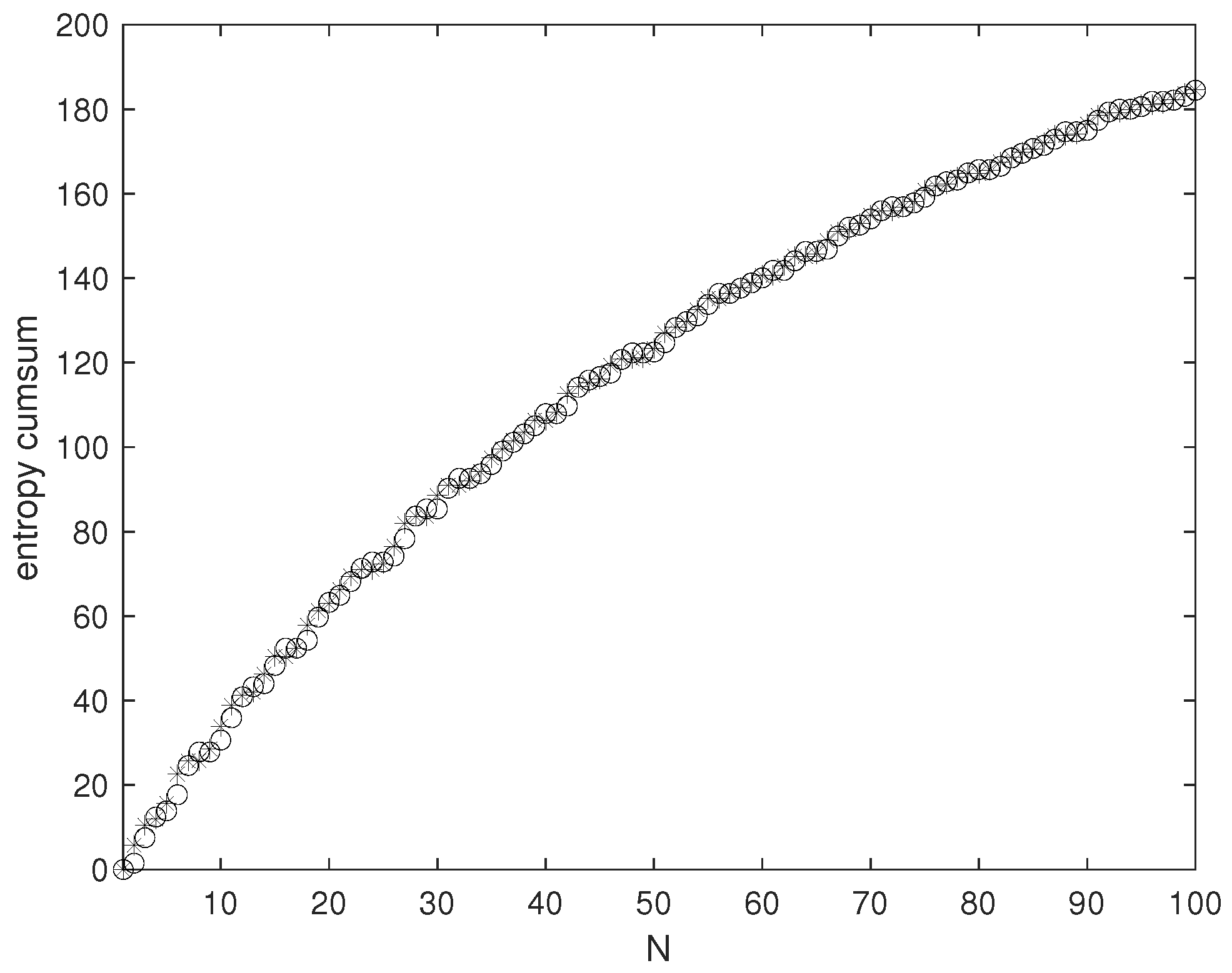
Figure 2. Entropy distribution

S_{r_{n}}

obtained using the smooth multiplicity

g_{n} = π \sqrt{n} / 4

. Temperature 300 Kelvin, side of the box

6 \cdot 10^{- 5}

meters. Asterisks: geometric distribution. Circles: Poisson distribution. Crosses: rightmost term of (25).

Figure 2. Entropy distribution

S_{r_{n}}

obtained using the smooth multiplicity

g_{n} = π \sqrt{n} / 4

. Temperature 300 Kelvin, side of the box

6 \cdot 10^{- 5}

meters. Asterisks: geometric distribution. Circles: Poisson distribution. Crosses: rightmost term of (25).

Disclaimer/Publisher’s Note: The statements, opinions and data contained in all publications are solely those of the individual author(s) and contributor(s) and not of MDPI and/or the editor(s). MDPI and/or the editor(s) disclaim responsibility for any injury to people or property resulting from any ideas, methods, instructions or products referred to in the content.

© 2024 by the authors. Licensee MDPI, Basel, Switzerland. This article is an open access article distributed under the terms and conditions of the Creative Commons Attribution (CC BY) license (http://creativecommons.org/licenses/by/4.0/).

Copyright: This open access article is published under a Creative Commons CC BY 4.0 license, which permit the free download, distribution, and reuse, provided that the author and preprint are cited in any reuse.

Downloads

Views

Comments

Subscription

Notify me about updates to this article or when a peer-reviewed version is published.

MDPI Initiatives

Important Links

Choose an area of interest and we will send you notifications of new preprints at your preferred frequency.

Disclaimer

Derivation of Bose’s Entropy Spectral Density from the Multiplicity of Energy Eigenvalues

Abstract

Keywords:

Subject:

1. Introduction

2. Multiplicity of Energy Eigenvalues and Density of States

3. Energy Spectral Density and Entropy Spectral Density of the Photonic Thermal State

4. Comparison with Other Derivations

5. Comparison with the Poisson Distribution of the Occupancy Numbers

6. Conclusion

Funding

Data Availability Statement

Acknowledgments

Conflicts of Interest

References

MDPI Initiatives

Important Links

Subscribe