Submitted:
14 May 2024
Posted:
16 May 2024
You are already at the latest version
Abstract
The Lobo reservoir designed to supply water to the Daloa city populations (Central west of Côte d'Ivoire) is facing the phenomenon of eutrophication due to the agricultural plots located upstream the reservoir inputs. Studies have highlighted the reservoir pollution and sedimentation problem. This study was initiated to provide a simple and effective solution to the eutrophication problem. The main objective is to determine the potential optimal dimensions of a grassed strip in order to limit the eutrophication phenomenon of the Lobo reservoir. The sizing of this grassed strip was done using the VFSMOD model. The flow from the pollution source plots was simulated and integrated into the model. The different scenarios tested from the band width variation have concerned the return periods of 1 and 2 years. The results obtained revealed that for the one-year return period, the grassed strip to be installed should have a width of 12.70 m in order to reduce by 70% the flow entering the strip considering the diffuse runoff over a length of 300 m. For the two-year return period, a width of 22.95 m should be required with the same length. The scenarios showed that a grassy strip width equal to 3 m should allow a reduction of 75% of upstream sediments.
Keywords:
Grass strip
; eutrophication
; pesticides
; pollution
; protection
; VFSMOD
; Lobo
; Côte d'Ivoire
1. Introduction
Improving the living conditions of populations requires better access to basic services, particularly the availability of drinking water. The State of Côte d’Ivoire, like the States of Sudano-Sahelian Africa, has so well understood the challenges of access to clean water, that it initiated with the support of development partners’ actions aimed at facilitating access to the public drinking water service for the greatest number of Ivoirians. From this political will, numerous dams were built during the 1970s and 1980s [1]. However, in recent years, we have observed for most of these dams, particularly those located in agricultural areas, processes of degradation and filling of the water bodies that they constitute following early eutrophication phenomenon [2]. Indeed, demographic pressure has led to a sharp increase in cultivated areas [3] and has expanded the consumer market for food and industrial products. To meet this strong demand and protect their crops, the State of Côte d’Ivoire, through structures such as ANADER (National Rural Development Support Agency), encourages traditional farmers and even industrialists to use agricultural inputs (fertilizers and pesticides). However, the lack of training on the sustainable use of agricultural inputs and the non-compliance with the principles of environmental protection with regard to these inputs, have caused an exacerbated use of these products which end up in the hydrographic network, causing eutrophication problems [4]. The case of the Lobo reservoir highlighted by Maïga et al. [5] is representative.
Thus, runoff water transports particles, pesticides and fertilizers remaining on the ground, not used by plants. Excess pesticides and agricultural inputs drained by leaching phenomena mainly contain nitrates and phosphates [6] which are nutrients for algae growing on the reservoir. On the one hand, a small increase in algae biomass has no effect on the ecosystem and can even cause an increase in certain fish populations. On the other hand, when there are too many nutrients in the water, too strong stimulation of algae growth can ultimately cloud the water. When the algae die, it is decomposed by numerous bacteria which use the oxygen in the water to breathe, causing a lack of dissolved oxygen in the aquatic environment; which threatens the survival of other living beings and of the reservoir itself [7]. The Lobo reservoir is used by the Cote d’Ivoire Water Distribution Company (SODECI) to supply drinking water to the Daloa town populations and its surrounding areas as well as to meet the water needs of agropastoral activities. The work carried out by Koua et al. [8], Soro et al. [9], N’goran et al. [10] showed a spatial distribution of nutrients from mineral fertilizers applied to plants. This distribution predisposes ivorian reservoirs, particularly the Lobo reservoir to an enrichment of nutrient elements responsible for the observed eutrophication phenomenon in that reservoir. In view of its certain interest, the contamination of this water resource by the use of pesticides and fertilizers used in agriculture, added to poor agricultural practices (slash-and-burn cultivation, soil left bare between two crops, etc.) constitutes a problem worrying for its users. Faced with this situation, it is essential to find more effective systems for reducing pollution and determine the best way to reproduce them in order to preserve water resources, hence the interest of this study using the VFSMOD (Vegetative Filter Strip Modeling) model. The development of grass strip techniques in Cote d’Ivoire is still in its embryonic state. The proposal of this technique for the fight against eutrophication of water bodies in Cote d’Ivoire is one of the research perspectives of the thesis work of Koua [11].
The objective of this study is to determine the optimal dimensions of a grassy strip in order to limit the eutrophication phenomenon of the Lobo.
2. Materials and Methods
2.1. Materials
2.1.1. Study Site
The Lobo reservoir is located 25 km from the town of Daloa between Longitudes 6°2 and 7°55 West and Latitudes 6° and 6°55 North (Figure 1). It belongs to the Lobo watershed with an area of 7280 km2. The city of Daloa represents the economic center of the region [12]. The Lobo River is one of the main tributaries on the left bank of the Sassandra River. The average flow of the river at the Nibéhibé hydrometric station is 12.43 m3.s-1 [13].
The climate of the basin is attenuated transitional equatorial type. The seasons are divided between a rainy season from March to October with a slowdown in precipitation in July and peaks observed in June and September, and a dry season from November to February with some isolated precipitation. Dry and wet seasons alternate with temperatures varying from 25.6°C to 28.65°C on average. Over the period 2000-2017, average interannual rainfall of 1246 mm was observed at the Daloa station.
The relief of the basin is not very rugged and consists of plains and low plateaus [14]. The plains whose altitude varies between 180 and 250 m are located in the south of the basin and correspond to the watercourse route. The hydrographic network of the Daloa region (Figure 2) is dominated by the Sassandra River. The Lobo, the main tributary of the Sassandra, is the second most important river. The large rivers, the Dê and the Gôré complete the hydrographic picture of the Daloa region [12]. All these watercourses have large alluvial plains along their courses suitable for irrigated crops and other off-season vegetable crops. In dry periods, the very sharp drop in water levels and the river beds sometimes leave wide hollows interspersed with puddles. The waters of the Lobo flow mainly in the north-south direction and the period of lowest water is observed during the first months of the year (January and February). The annual maximum rainfall is observed in September or October [12].
The geological formations encountered in this area, mainly made up of magmatic rocks, are of plutonic and volcanic types [15].
Hydrogeologically, the basin is located in a crystalline basement zone. There are two types of aquifers: alterite aquifers (superficial) and fractured aquifers deeper than the previous ones [16]. The estimated annual recharge varies from 66.4 to 84 mm respectively in 2019 and 2020. As for the average direct recharge, it is estimated respectively at 44 mm in 2018 and 57.3 mm in 2019, or respectively approximately 4% and 5% of precipitation [17]
2.1.2. Data
To carry out this study, agronomic, soil and climatic data were used. These are among others:
- the soil properties of the source of pollution (the degree of compaction, grain size and structure of the soil) from the FAO (Food and Agriculture Organization of the United Nations) database [18], the potential location of the grassy strip and land use (different crops grown in the source of pollution area);
- the average concentration of sediment entering the reservoir from April to December 2019 provided by the LSTE (Laboratory of Environmental Sciences and Technology) of Jean Lorougnon Guede University;
- rainfall and temperature data from the Daloa station at daily time intervals from 2000 to 2017 provided by SODEXAM (the Aeronautical and Meteorological Development and Exploitation Company).
2.1.3. Work Tools
The tools used to process the data consist of Microsoft Excel for processing rainfall data and for producing graphs and diagrams, the “Soil Water Characteristics” program included in SPAW (Specially Protected Areas and Wildlife) to simulate conductivity and the water retention capacity of the soil, VFSMOD-W software (Vegetative Filter Strip Modelling, Window system) to model the scenarios and define the optimal dimensions of the grassy strip, Google Earth which allowed the extraction of topographical dimensions along the potential source of pollution and ArcGis 10.4 to produce the different maps and determine the dimensions of the pollution source (contributing area).
2.2. Methods
The methodology adopted in this study is mainly based on the VFSMOD transfer model.
2.2.1. Description of the VFSMOD Model
The VFSMOD model was developed in United States of America by Muñoz-Carpena & Parsons [19]. VFSMOD is a plot-scale storm-based mechanistic model designed to route the incoming hydrograph and sedimentograph from an adjacent plot through a filtering vegetation strip and to calculate its effectiveness on flow, infiltration and trapping of sediments. The model handles time-dependent hyetographs, spatially distributed filter parameters (vegetation roughness or density, slope, infiltration characteristics) and different particle sizes of incoming sediments. Any combination of unstable storm types and incoming hydrographs can be used. VFSMOD consists of a series of modules simulating the behavior of water, sediments and pollutants across the grassy strip. The modules currently available are: i) infiltration module: a module for calculating excess precipitation and water balance at the ground surface for unbounded deep soils or shallow waters; ii) kinematic wave surface flow module: a 1-D module for calculating the depth and flow rates at the surface of the filter soil; iii) sediment filtration module: a module for simulating the transport and deposition of incoming sediments along the vegetative filter (VF). VFSMOD is essentially a 1-D model for describing water transport, sediment deposition, and pollutant trapping along the VF. This model has different components: hydrology, sediment and chemical transport.
- -
- Hydrology
In the hydrological component, it involves solving the kinetic wave approximation of the Saint-Vennant’s (1881) equations for overland flow (KW) for the 1-D case as presented by Lighthill and Whitham [20] such as:
Then, based on the Manning equation, a link between q and h can be established to define a uniform flow equation:
where h is depth of overland flow [L], q is the flow per unit width of the plane [L2T-1], So is the slope of the plane, Sf is the hydraulic or friction slope, and n is Manning’s roughness coefficient [LT-1/3]. The initial and boundary conditions can be summarized as:
where ho can be 0, a constant or a time dependent function, such as the incoming hydrograph from the adjacent field.
It also represents a link to measured data or other water quality models describing incoming runoff and pollutants from the source area..
- -
- Sediment and chemical transport
A filtration of suspended matter model using artificial turf was developed and then tested for field conditions [21,22,23,24,25,26,27]. It is also based on the hydraulics of flow, transport and deposition profiles of sediments in laboratory conditions. The model has the advantage of being developed specifically for the filtration of suspended matter by grass.
The advantage of VFSMOD over other models used to simulate pollution removal is the inclusion of filter hydrology, including flow changes derived from sediment deposition, soil water infiltration depending on time, management of complex sub-models and intensity of storms and variable surface conditions (slope and vegetation) along the filter. The model aims to study VF performance on an event-by-event basis and becomes a powerful and objective design tool. The design paradigm implemented in VFSMOD seeks to identify the optimal constructive characteristics of the filter (length, slope, vegetation) to reduce (to a reduction objective prescribed as Total Maximum Daily Load) the output of pollutants from a given disturbed area (soil, cultivation, management practices, etc.). VFSMOD has been tested in a wide variety of contexts (agroforestry, mining and roads) with good model predictions against measured values of infiltration, runoff and vegetation trapping efficiency for sediments, phosphorus (particulate and dissolved), nitrates and pesticides. Indeed, Sur et al. [28] used it to implement effects of shallow water table on pesticide runoff mitigation effectiveness. Similarly, Minwoo et al. [29] conducted a study on the trapping efficiency of diffuse pollution source in Cheongmi Stream using VFSMOD. In the same direction, Muñoz-Carpena et al. [30] analyzed the effectiveness of the VFSMOD model during long-term exposure of pesticide residues in vegetative filter strips.
2.2.2. Steps
The methodological approach is structured into four (4) main stages:
- Evaluation of runoff from the source of pollution (contributing surface) during a rainy episode;
- Calculation of the incoming sediment load;
- Simulation of runoff reduction and incoming sediments within the grassy filter strip;
- Determination of the optimal dimensions of the grassy strip.
Evaluation of runoff from the pollution source (contributing area) during a rainy episode
This step first begins with determining the geometry of the contributing surface and choosing the rainy event. The length and surface area of the pollution source was determined using the “Measure” tool in ArcMap. Google Earth allowed the extraction of topographic coastlines in the direction of rainwater flow in order to calculate the average slope. For the dimensioning of this buffer strip, one choses the height of the maximum daily rainfall over the period 2000-2017. This height corresponds to 121 mm. Then, the construction of the unit hydrograph (UH) was carried out. Indeed, the Curve Number (CN) is an empirical parameter, used in hydrology to predict direct runoff or infiltration from excess precipitation [31]. The value of the Curve Number is chosen according to the hydrological group of the soil, the land use, the hydrological conditions and the initial humidity conditions of the environment. To simulate the rainy event, the corresponding runoff events from the contributing surface, the use of the “Hydrogram Unit” module in VFSMOD was necessary. This is based on the use of the SCS-CN method to generate the unit hydrograph. The data provided are: the cumulative rainfall amount, the duration of the event, the CN, the dimensions of the pollution source area, the erosion parameters in particular the erodibility of the soil and the soil type. The SCS-CN method was developed by the USDA-NRCS (US Department of Agriculture–Natural Resources Conservation Service) to predict runoff volume [32]. For a given rainfall event, the runoff volume is calculated using Equations (1) and (2):
with:
Q= 0, if P≤ Ia
- Q (mm) is the direct runoff,
- P (mm) is the cumulative precipitation,
- Ia (mm) are the initial losses,
- S (mm) is the soil retention.
Soil retention and initial losses are calculated using the following equations:
In this method the runoff hydrograph (UH) which represents the evolution of the runoff flow as a function of time makes it possible to directly evaluate the runoff from the knowledge of the rainfall and the curve number and the synthetic hydrograph. For this it is necessary to calculate the watershed delay time L, the peak time Tp and the peak flow Qp according to the physical characteristics of the watershed studied. It is not necessary to calculate the concentration time Tc if these three quantities are determined [33].
The watershed delay time L is calculated using the following equation:
with:
- L (h) is the delay time,
- l (m) is the longest hydraulic path,
- S (mm) is the maximum soil retention,
- Y (%) is the average slope of the watershed.
The peak time Tp of the unit hydrograph is calculated using the following equation:
where,
- Tp (h) is the peak time,
- ∆D (h) is the elementary shower duration,
- L (h) is the watershed delay time.
As for the peak flow Qp, it is estimated according to Equation (7):
where A (km²) is the drained area.
The hyetogram (temporal evolution of rain quantities) of net rain was then constructed. It is based on the determination of the volume of net rain associated with each of these elementary showers [33], that is to say the part of rain which will contribute directly to the runoff genesis (the remainder being infiltrated or stored in the microtopography of the soil). For this study, we use the equations of Chow et al. [34]:
with:
Ia = Ia, if P > Ia
- R (mm) is the cumulative net rain,
- P (mm) is the cumulative rain,
- Ia (mm) are the cumulative initial losses,
- F (mm) is the cumulative infiltration.
To determine the net rain associated with each elementary shower, it is sufficient to successively subtract the cumulative values obtained for each time interval [33].
R = P – Ia – F
Ia = P, if P < Ia
Calculation of incoming sediment load
The quantity of sediment entering the strip was calculated from the MUSLE model [35]; it is the modified version of the USLE model (universal soil loss equation) which evaluates water erosion during flooding based on five erosion factors. The equation is given by Equation (12):
where,
A is the sediment load (tons);
α = 11.8 and β = 0.56 are two parameters of the MUSLE model;
Q is the volume of runoff (m3);
qp is the peak flow (m3.s-1) during the flood;
K is the soil erodibility factor (thMJ−1mm−1);
LS is the topographic factor (unitless);
C is the plant cover management factor (unitless);
P is the anti-erosion development factor (unitless).
At the end of all these steps, two (2) files are created and saved. A file containing information on the contributing surface area and another including information on the grassy strip and the soil characteristics of its potential location.
Simulation of runoff and incoming sediments reduction within the grassy strip
Simulation is a technique for explicitly reproducing any process. In this study, the “Grass device (VFS)” module in VFSMOD was used to simulate runoff reduction within the strip. The modeling approach is as follows:
- integrate the runoff previously assessed and the hyetogram of the event into the VFSMOD model;
- provide information on the soil and the incoming sediments properties;
- execute the program for reducing the flow entering the grassy strip.
This simulation based on a width of 3 m will be used for sizing the grass strip.
Determination of the grass strip optimal dimensions
The sizing of the strip was carried out using the “Design Analysis” module in VFSMOD. The two (2) files containing information on the contributing area and the grass strip are used. The scenarios are obtained from several simulations which combine data from the contributing surface area and the infiltration capacities of the simulated grass strip. The parameters to be entered are the duration of the downpour which is one (1) hour recommended by Carluer et al. [33] and the return period. To intercept fairly common events, the choice of return periods of one (1) year and two (2) years is necessary. The estimation of flow rates for the return periods was done by the statistical method using Gumbel’s law. According to Kouassi et al. [36], Gumbel’s law seems well suited to the equatorial transition regime.
The distribution function of Gumbel’s law F(x) is expressed by Equation (13):
with the following reduced variable:
the distribution is then written as follows:
Then,
The expression for a quantile is then linear:
a and b are the parameters of the Gumbel model.
The return time T of an event is defined as being the inverse of the event occurrence frequency:
The calculation of T is done at the watershed scale by retaining the values linked to the study site by extrapolation.
The evaluation of the effectiveness of the grass strip was carried out over an interval of 3 to 30 m of grass strip width with an increment of 1 m. Beyond 30 m, it is considered that the footprint of the device is too large and that it is not likely to respond effectively to the problem of runoff. Thus, the flow of water generated by the contributing zone becomes too large to be “absorbed” by the grassy strip [31]. The scenarios resulting from the sizing are analyzed and the dimensions which allow a significant reduction in runoff according to the desired objective are retained. These dimensions are called optimal dimensions. In our study the objective is to reduce incoming runoff by 70%.
3. Results
3.1. Geometry of the Contributing Surface Area (Source of Pollution)
The source of pollution has an area of 0.135 km2 or 13.5 ha for an average length of 645 m. From upstream to downstream, the slopes vary between 2.7% and 0.4%. The average slope is 2%. The contributing area extends over a width of 210 m on average. The longest hydraulic path is 519 m.
3.2. Unit Hydrograph (UH) of the Contributing Area
The results of the flow variation as a function of time are presented in Figure 3. The flood hydrograph has the shape of an asymmetrical bell curve on which four parts are observed: drying up (before the net rain) AB, flood BC, CD recession and drying up (after the hydro-rainfall survey) DE.
The characteristic times obtained are: the rise time Tm, that is to say the time which elapses between the arrival at the grassy strip of the rapid flow and the maximum of the hydrograph, i.e., 30.97 minutes; the basic time Tb which corresponds to the duration of runoff, i.e., 69.7 minutes. The volume of net rain (runoff volume) is 4680 m3.
Knowing that, the contributing surface area is 0.135 km2, and the total amount of water runoff is 35 mm, or 29% of the rain that fell.
3.3. Hyetogram of the Contributing Area
Figure 4 illustrates the evolution of rain intensity over time. The rain event considered for this study lasts one (1) hour. The maximum intensity is observed at approximately 31 minutes. This distribution describes a normal law with a peak of 13.77.10-5 m.s-1.
3.4. Runoff and Sediment Entering the Grassy Strip Trapping
The results show that a grassy strip 3 m wide reduces the incoming water flow by 1118.52 m3, or a reduction of 24% in the volume (4680 m3) coming from the source of pollution (Figure 5).
3.5. Optimal Dimensions of the Grass Strip under Different Scenarios
Figure 7 presents the effectiveness curves of the grass strip in limiting surface runoff as a function of its width according to the return periods (one year T1 and two years T2). It appears that the greater the width of the strip, the greater the reduction in runoff.
The sediment load goes from 131.75 kg to 32.94 kg, a reduction of 75% in the quantity of sediment entering (Figure 6).
Figure 6.
Reduction of sediment load before simulation.
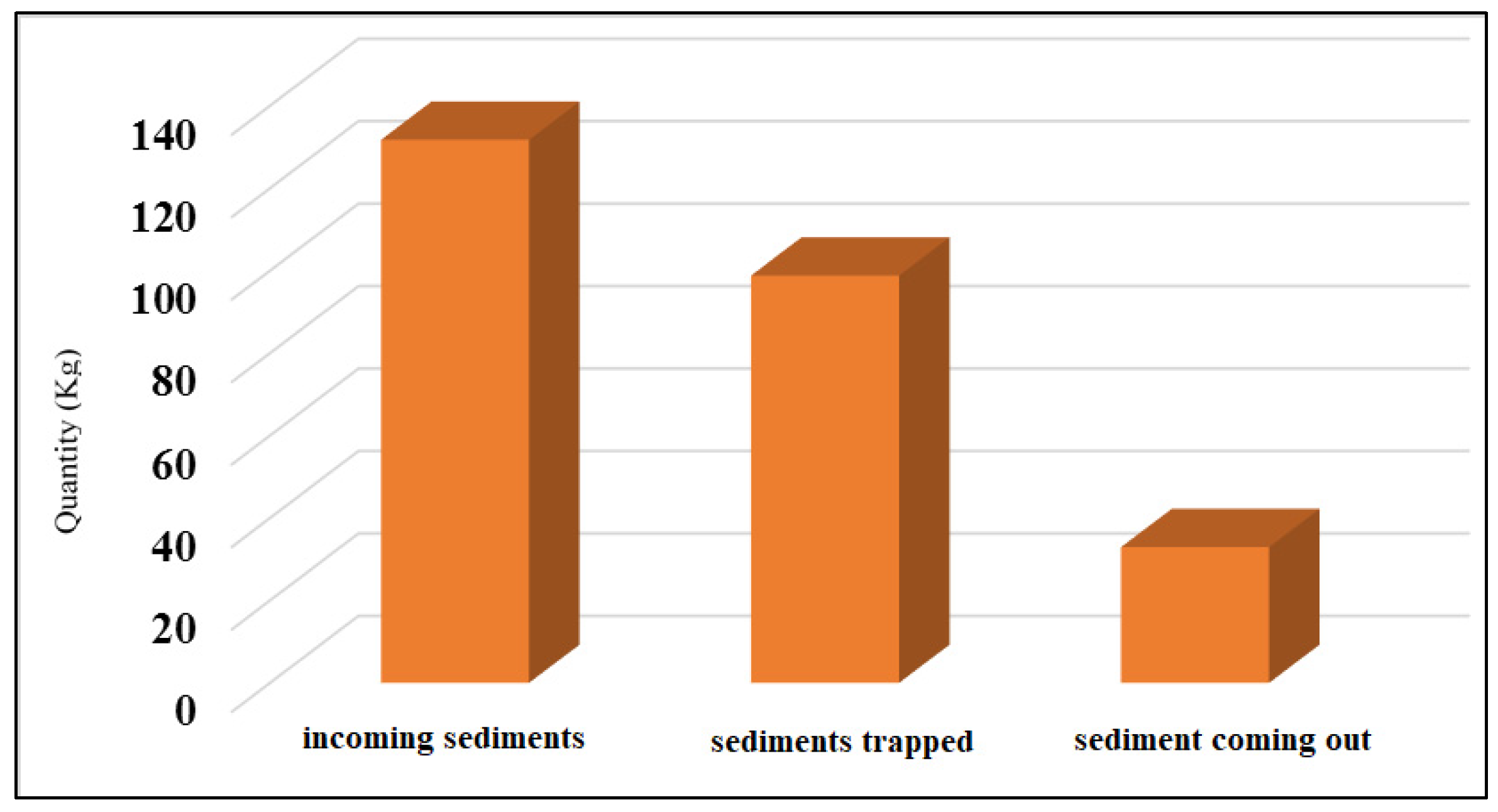
Figure 7.
Evolution of the outgoing runoff ratio as a function of the width of the strip.
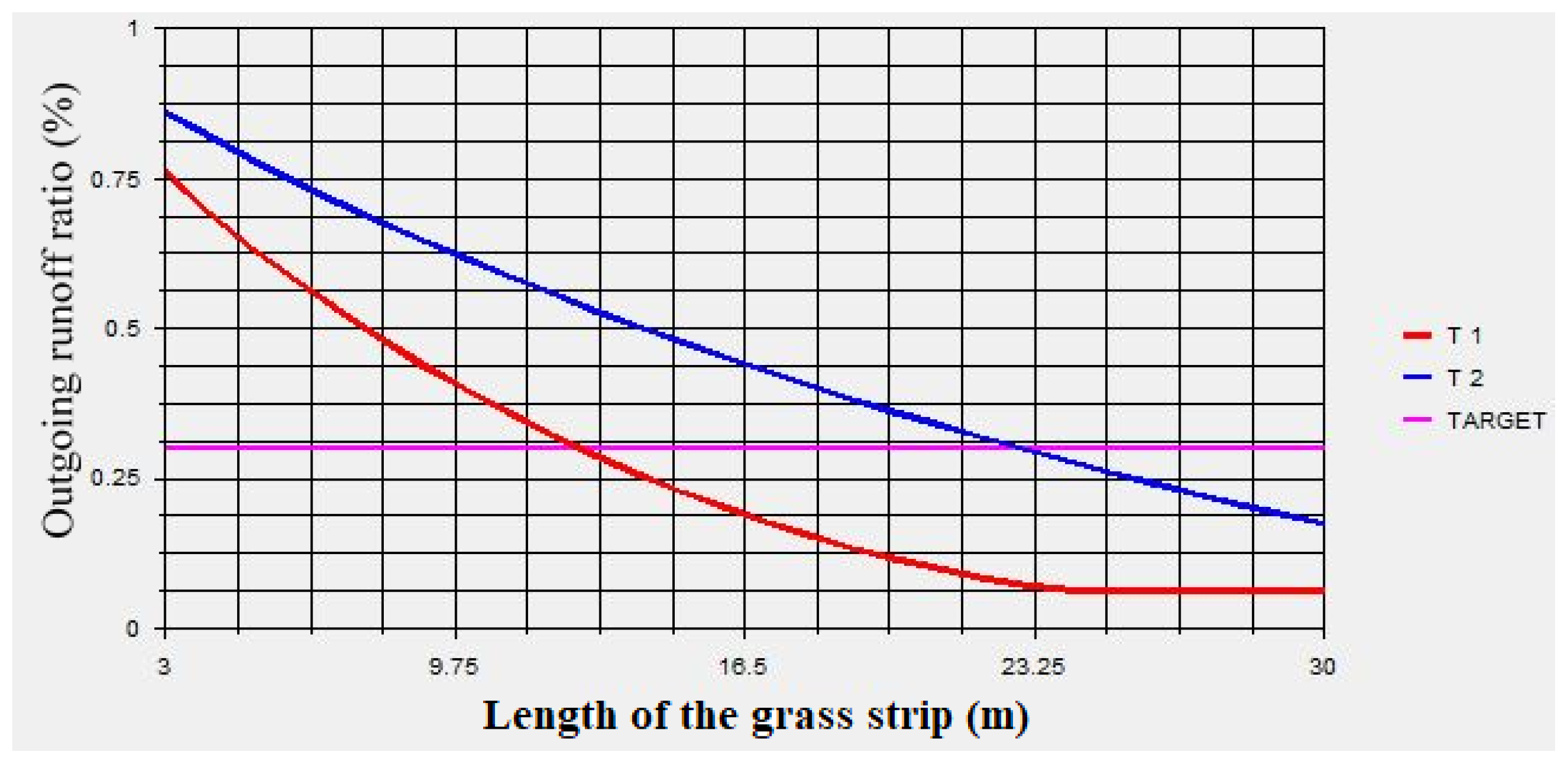
This observation is valid for the two (2) return periods. The T1 curve, however, shows that simulated grassy strips with a width greater than 24 m have an almost identical retention capacity.
The percentage of effectiveness sought in this study was 70%, or an output ratio of 30%. The analysis of the results of each scenario made it possible to find the optimal dimensions of the grassy strip according to the objective sought in this study. These are shown in Table 1.
Figure 8 shows the effectiveness of the grass strip, modeled in this study for the reduction of diffuse runoff and sediment flows. For a runoff of 35 mm, 24.5 mm is infiltrated and 10.5 mm joins the reservoir (Figure 8a); and for a quantity of 131.7 kg of sediment, 128.4 kg is retained by the band and only 3.3 kg comes out (Figure 8b).
4. Discussion
This study is carried out with the aim of modeling a grassy strip effective against the transfer of pollutants by runoff towards the Lobo reservoir. The result is that only 3 m of grassy strip width is needed to reduce the polluting load by 75%. Remember that this runoff occurs diffusely over a length of 300 m. This result differs from that proposed by Dosskey et al. [37]. These authors did not propose a buffer strip width, but rather a buffer area ratio which corresponds to the division of the effective grassy strip area by the area of pollution source. Thus, it is no longer a question of establishing a buffer strip width, but rather the surface area that runoff water must cross for a certain part to be captured [38]. According to Dosskey et al. [37], a ratio of 1% should be used to reduce the volume of water runoff from the plot studied by 60-75% for the same duration of downpour (1 hour), i.e., a width of 4.5 m for a length of 300 m. The width suggested by the latter is greater than that obtained in our study. This difference in value can be explained by the parameters taken into account by each of these models. In regions with a cold climate, such as Quebec, which are distinguished by a specific problem linked to the melting of snow in spring which generates significant water erosion at a time when the vegetation is dormant, their effectiveness is however variable [39,40]. It depends on the type of pollutants, local conditions, their location in the hydrographic network but also their width and composition [41,42]. Unlike the tool proposed by Dosskey et al. [37] which is based on only three parameters, notably the slope, the texture of the soil and the land use type, the VFSMOD model takes into account, in addition to the aforementioned parameters, the coverage plant of the strip. The plant density makes it possible to reduce the speed of runoff [43,44] and therefore the energy available for the transport of particles and to limit erosive phenomena on the grassed device itself, in the soil as well as the sedimentation of particles upstream of the grass strip.
The results also show that for a return period of one (1) year, a width of 12.47 m is necessary to reduce the volume of water runoff by 70%, or 35 mm. On the other hand, for a period of two (2) years, it will be necessary to put in place a strip of 22.95 m to achieve the objective of 70% reduction. We note that the reduction in the solid load is much greater than that of the runoff volume and that a wider band is required to reduce the flow of rainwater runoff. These results confirm the experimental results of Borin et al. [45]; these experiments carried out over 4 years using natural rainfall have shown that the performance of grassed devices in reducing the sediment load is 10-15% higher than that allowing runoff to be reduced with the same filtering width. This difference in performance is explained by the fact that the volume runoff is much greater than the quantity of particles transported. In the case of this study for example, we have 4680 m3 of water arriving on the grassy strip compared to 131.75 kg of sediment.
The different simulation scenarios obtained result from a width range of 3 to 30 m. The observation is that variations in bandwidth lead to variability in performance. Runoff retention ranges from 24 to 93.8%. These results show that the performance of the grass strip in reducing the incoming flow does not evolve in a linear manner. However, the wider the band, the more effective it is; These results are consistent with the assertion of Schmitt et al. [46] according to which doubling the width of the grassy strip, in this case from 7.5 to 15 m, causes a net reduction in the concentrations and fluxes of all dissolved contaminants. Indeed, pesticides are transported mainly in dissolved form [6]. Therefore, the greater the distance traveled by runoff in the grassy area, the higher the infiltration and adsorption potential. This situation is favored by the root system of plants and by the reduction in flow speed due to the roughness of the plant cover [47]. However, beyond 25 m, the efficiency is constant despite the increase in width. This could be explained by the clogging of the grassy system; the available porosity of the soil is less and less important, limiting the infiltration of the runoff water quantity.
The Model used for this work made it possible to determine the possible dimensions for an effective reduction of contaminants transported by runoff towards the Lobo reservoir. However, the fate of phytosanitary products infiltrated into the soil (retention and degradation or deep transfer) is not considered in this work. The model simulates runoff and its interception by the buffer strip for a rainy episode and given initial conditions. It is therefore not possible to carry out a continuous simulation over a succession of episodes based on this model.
5. Conclusions
The different scenarios obtained from the VFSMOD model, have resulted from a variation in the width of the vegetative filter strip (VFS) for each chosen return period. A scenario corresponds to a set of input parameters (characteristics of the contributing surface, incoming flow, soil properties where the strip will be positioned, the slope of the area) for which the vegetative filter strip dimensions were determined, that is to say the width as a function of the reduction rate. The VFS efficiency calculations were carried out for widths varying from 3 to 30 m with an increment of 1 m. It has emerged from the analysis of the results obtained after simulation, that for a return period of one (1) year, the VFS to set up must have a width of 12.70 m in order to reduce the incoming flows by 70% considering diffuse runoff over a length of 300 m. For a return period of two (2) years, a width of 22.95 m is necessary. Regarding particles transported by runoff, the scenarios showed that a 3 m wide grassy strip would allow a 75% reduction in these sediments. This work was able to confirm the effectiveness of a grassy strip in limiting the transfer of pollutants to the Lobo reservoir with the aim of reducing the eutrophication of this important and vital resource for the Daloa’s population and its surroundings.
Author Contributions
Conceptualization, T.J.-J.K.; methodology, T.J.-J.K.; software, T.J.-J.K. and K.A.A; validation, T.J.-J.K., K.H.K. and K.L.K.; writing—original draft preparation, T.J.-J.K.; writing—review and editing, T.J.-J.K., K.H.K. and K.L.K.; supervision, T.J.-J.K.; project administration, K.L.K.; funding acquisition, T.J.-J.K. All authors have read and agreed to the published version of the manuscript.
Funding
This research was funded in part by J. William Fulbright Foreign Scholarship program, grant number PS00285574.
Data Availability Statement
All the data used in this paper can be traced back to the cited references.
Acknowledgments
The authors would like to thank Professor R. Muñoz-Carpena from the University of Florida in Florida (Gainsville, USA), designer of the VFSMOD Model, for his availability and his coaching which enabled the effective use of the model.
Conflicts of Interest
The authors declare no conflict of interest.
References
- Koukougnon, W.G. Milieu urbain et accès à l’eau potable: Cas de Daloa (Centre-Ouest de la Côte d’Ivoire). Thèse Unique de Doctorat, Université Félix Houphouet Boigny Abidjan, Cote d’Ivoire, 2012; 323p. [Google Scholar]
- Komelan, Y. Eutrophisation des retenues d’eau en Côte d’Ivoire et gestion intégrée de leur bassin versant: cas de la Lobo à Daloa. Mémoire de master, École d’Ingénieurs de l’Équipement Rural de Ouagadougou, Ouagadougou, Burkina Faso, 1999; 56p. [Google Scholar]
- Floret, C. (IRD, Dakar, Sénégal); Hien, V. (INERA, Ouagadougou, Burkina Faso); Pontanier, R. Le projet « La jachère en Afrique tropicale ». Personal communication, 1993.
- Koua, T.J.-J.; Dhanesh, Y.; Jeong, J.; Srinivasan, R.; Anoh, K.A. Implementation of the Semi-Distributed SWAT (Soil and Water Assessment Tool) Model Capacity in the Lobo Watershed at Nibéhibé (Center-West of Côte D’Ivoire). J. Geosci. Environ. Prot. 2021, 9, 21–38. [Google Scholar]
- Maïga, A.; Denyigba, K.; Allorent, J. Eutrophisation des Petites Retenues d’eau en Afrique de l’Ouest: Causes et Conséquences: Cas de la Retenue D’eau de la Lobo en Côte d’Ivoire. Sud Sci. Technol. 2001, 7, 16–29. [Google Scholar]
- Lecomte, V. Transfert de produits phytosanitaires par le ruissellement et l’érosion de la parcelle au bassin versant. Thèse de doctorat, École Nationale du Génie Rural des Eaux et des Forêts de Montpellier, Montpellier, France, 1999. [Google Scholar]
- Peter, G.V.; Brussaard, C.P.; Nejstgaard, J.C.; Van Leeuwe, M.A.; Lancelot, C.; Medlin, L.K. Current understanding of Phaeocystis ecology and biogeochemistry, and perspectives for future research. Biogeochemistry 2007, 83, 311–330. [Google Scholar]
- Koua, T.J.-J.; Jeong, J.; Alemayehu, T.A.; Dhanesh, Y.; Srinivasan, R. Spatial Distribution of Nutrient Loads Based on Mineral Fertilizers Applied to Crops: Case Study of the Lobo Basin in Côte d’Ivoire (West Africa). Appl. Sci. 2023, 13, 9437. [Google Scholar] [CrossRef]
- Soro, M.-P.; N’goran, K.M.; Ouattara, A.A.; Yao, K.M.; Kouassi, N.L.; Diaco, T. Nitrogen and phosphorus spatio-temporal distribution and fluxes intensifying eutrophication in three tropical rivers of Côte d’Ivoire (West Africa). Mar. Pollut. Bull. 2023, 186, 114391. [Google Scholar] [CrossRef] [PubMed]
- N’goran, K.M.; Soro, M.-P.; Kouassi, N.L.B.; Trokourey, A.; Yao, K.M. Distribution, Speciation and Bioavailability of Nutrients in M’Badon Bay of Ebrie Lagoon, West Africa (Côte d’Ivoire). Chem. Afr. 2023, 6, 1619–1632. [Google Scholar] [CrossRef]
- Koua, T. Apport de la Modélisation Hydrologique et des Systèmes d’Information Géographique (SIG) dans L’étude du Transfert Des Polluants et des Impacts Climatiques sur les Ressources en eau: Cas du bassin Versant du lac de Buyo (Sud-ouest de la Côte d’Ivoire). Ph.D. Thesis, Felix Houphouet Boigny University of Cocody, Abidjan, Côte d’Ivoire, 11 December 2014. [Google Scholar]
- Yao, A.B. Evaluation des potentialités en eau du bassin versant de la Lobo en vue d’une gestion rationnelle au Centre-Ouest de la Côte d’Ivoire. Thèse de Doctorat, Université Nangui Abrogoua, Abidjan, Côte d’Ivoire, 2015. [Google Scholar]
- Koffi, B.; Kouassi, K.L.; Sanchez, M.; Kouadio, Z.A.; Kouassi, K.H.; Yao, A.B. Estimation de la sédimentation dans la retenue d’eau de la rivière Lobo à l’aide de la théorie des bassins de décantation. In Proceedings of the XVIèmes Journées Nationales Génie Côtier – Génie Civil, Daloa, Côte d’Ivoire, 8–10 Décembre 2020. [Google Scholar]
- Brou, T.; Akindès, F.; Bigot, S. La variabilité climatique en Côte d’Ivoire: entre perceptions sociales et réponses agricoles. Cahiers Agricultures 2005, 14, 533–540. [Google Scholar]
- Delor, C.; Siméon, Y.; Vidal, M.; Zeade, Z.; Koné, Y.; Adou, M.; Dibouahi, M.; Irié, D.B.; N’da, B.D.; et al. Carte géologique de la Côte d’Ivoire à 1/200 000, feuille Nassian. Mémoire n°9 de la Direction des Mines et de la Géologie, Côte d’Ivoire, 1995.
- Yao, A.B.; Bi Tié, A.G.; Kane, A.; Mangoua, J.O.; Kouamé, A.K. Cartographie du potentiel en eau souterraine du bassin versant de la Lobo (Centre-Ouest, Côted’Ivoire): approche par analyse multicritère. Hydrological Sciences Journal 2016, 61, 856–867. [Google Scholar]
- Jean Olivier, K.K.; Brou, D.; Jules, M.O.M.; Georges, E.S.; Frédéric, P.; Didier, G. Estimation of Groundwater Recharge in the Lobo Catchment (Central-Western Region of Côte d’Ivoire). Hydrology 2022, 9, 23. [Google Scholar] [CrossRef]
- Nachtergaele, F.; Velthuizen, H.V.; Verest, L. Harmonized world soil database version1.1. 2009. Available online: http://www.fao.org/3/aq361e/aq361e.pdf.
- Muñoz-Carpena, R.; Parsons, J.E. VFSMOD-W Vegetative Filter Strips Modelling System. MODEL DOCUMENTATION & USER’S MANUAL version 6.x. 2020; 194p. Available online: https://abe.ufl.edu/faculty/carpena/files/pdf/software/vfsmod/VFSMOD_UsersManual_v6.pdf.
- Lighthill, M.J.; Whitham, C.B. On kinematic waves: flood movement in long rivers. Proc. R. Soc. London Ser. A 1955, 22, 281–316. [Google Scholar]
- Barfield, B.J.; Tollner, E.W.; Hayes, J.C. The use of grass filters for sediment control in strip mining drainage. Vol. I: Theoretical studies on artificial media. Pub. no. 35-RRR2-78; Institute for Mining and Minerals Research, University of Kentucky: Lexington, 1978. [Google Scholar]
- Barfield, B.J.; Tollner, E.W.; Hayes, J.C. Filtration of sediment by simulated vegetation I. Steady-state flow with homogeneous sediment. Transactions of ASAE 1979, 22, 540–545. [Google Scholar] [CrossRef]
- Hayes, J.C.; Barfield, B.J.; Barnhisel, R.I. Filtration of sediment by simulated vegetation II. Unsteady flow with non-homogeneous sediment. Transactions of ASAE 1979, 22, 1063–1967. [Google Scholar] [CrossRef]
- Hayes, J.C.; Barfield, B.J.; Barnhisel, R.I. Performance of grass filters under Jackson, S.; Hendley, P.; Jones, R.; Poletika, N.; Russell, M. Comparison of regulatory method estimated drinking water exposure concentrations with monitoring results from surface drinking water supplies. J. Agr. Food Chem. 2005, 53, 8840–8847. Laboratory and field conditions. Transactions of ASAE 1984, 27, 1321–1331. [Google Scholar]
- Tollner, E.W.; Barfield, B.J.; Haan, C.T.; Kao, T.Y. Suspended sediment filtration capacity of simulated vegetation. Transactions of ASAE 1976, 19, 678–682. [Google Scholar] [CrossRef]
- Tollner, E.W.; Barfield, B.J.; Vachirakornwatana, C.; Haan, C.T. Sediment deposition patterns in simulated grass filters. Transactions of ASAE 1977, 20, 940–944. [Google Scholar] [CrossRef]
- Wilson, B.N.; Barfield, B.J.; Moore, I.D. A Hydrology and Sedimentology Watershed Model, Part I: Modeling Techniques; Technical Report; Department of Agricultural Engineering. University of Kentucky: Lexington, 1981. [Google Scholar]
- Sur, R.; Muñoz-Carpena, R.; Reichenberger, S.; Hammel, K.; Meyer, H.; Kehrein, N. Implementation of shallow water table effects on pesticide runoff mitigation efficiency by vegetative filter strips within SWAN-VFSMOD. EGU General Assembly 2021, 2021; 19–30 Apr, EGU21-7829. [CrossRef]
- Minwoo, S.; Jisun, B.; Hyun-Dong, Y.; Tae-Hwa, J. A study on trapping efficiency of the non-point source pollution in Cheongmi Stream using VFSMOD-W. The Journal of Korea Contents Association 2016, 16, 140–150. [Google Scholar] [CrossRef]
- Muñoz-Carpena, R.; Reichenberger, S.; Sur, R.; Hammel, K. Fate of pesticide residues in vegetative filter strips in long-term exposure assessments: VFSMOD development and analysis. EGU General Assembly 2021, 19–30 Apr 2021. 2021; EGU21-1735. [CrossRef]
- Catalogne, C.; Lauvernet, C.; Carluer, N. Guide d’utilisation de l’outil BUVARD pour le dimensionnement des bandes tampons végétalisées destinées à limiter les transferts de pesticides par ruissellement; Rapport de recherche IRSTEA: France, 2018; 66p, Available online: https://hal.inrae.fr/hal-02607260/document.
- USDA-SC. Design hydrographs. In National Engineering Handbook Hydrology, 2nd ed.; Vincent, M., William, O., Robert, R., Eds.; Departement of Agriculture: Whasington, D.C, USA, 1972; Available online: https://www.hydrocad.net/neh/630ch21.pdf.
- Carluer, N.; Fontaine, A.; Lauvernet, C.; Muñoz-Carpena, R. Guide de dimensionnement des zones tampons enherbées ou boisées pour réduire la contamination des cours d’eau par les produits phytosanitaires; Rapport de recherche IRSTEA: France, 2020; 72p, Available online: https://hal.inrae.fr/hal-02595578v1/file/pub00032826.pdf.
- Chow, V.T.; Maidment, D.R.; Mays, L.W. Applied hydrology, International Edition; Mc-Graw-Hill Book Company: USA, 1988; pp. 153–155. Available online: https://wecivilengineers.wordpress.com/wp-content/uploads/2017/10/applied-hydrology-ven-te-chow.pdf.
- Williams, J.R. Sediment-Yield Prediction with Universal Equation Using Runoff Energy Factor. In Proceedings of the Sediment-Yield Workshop, USDA Sedimentation Laboratory, Oxford, Mississippi, 28-30 November 1972. [Google Scholar]
- Kouassi, A.M.; Nassa, R.A.-K.; Yao, K.B.; Kouamé, K.F.; Biémi, J. Modélisation statistique des pluies maximales annuelles dans le district d’Abidjan (Sud de la Côte d’Ivoire). Revue des Sciences de l’Eau 2018, 31, 147–160. [Google Scholar] [CrossRef]
- Dosskey, M.G.; Helmers, M.J.; Eisenhauer, D.E. A design aid for sizing filter strips using buffer area ratio. Journal of soil and water conservation. 2011, 66, 29–39. [Google Scholar] [CrossRef]
- Breune, I.; Audet, M.A.; Parent, G. Le ray-grass intercalaire: Essai de variétés, Essai de semis à différents stades du maïs. Rapport final club agroenvironnemental de l’Estrie, Québec (Canada). 2015; 60p. Available online: https://www.agrireseau.net/documents/Document_90361.pdf.
- Kieta, K.A.; Owens, P.N.; Lobb, D.A.; Vanrobaeys, J.A.; Flaten, D.N. Phosphorus dynamics in vegetated buffer strips in cold climates: a review. Environ. Rev. 2018, 26, 255–272. [Google Scholar] [CrossRef]
- Hénault-Ethier, L.; Gomes, M.P.; Lucotte, M.; Smedbol, É.; Maccario, S.; Lepage, L.; Juneau, P.; Labrecque, M. High yields of riparian buffer strips planted with Salix miyabena ‘SX64’ along field crops in Québec, Canada. Biomass and Bioenergy. 2017, 105, 219–229. [Google Scholar] [CrossRef]
- Lind, L.; Hasselquista, E.M.; Laudona, H. Towards ecologically functional riparian zones: A meta-analysis to develop guidelines for protecting ecosystem functions and biodiversity in agricultural landscapes. Journal of Environmental Management. 2019, 249, 1–8. [Google Scholar] [CrossRef] [PubMed]
- Zhang, X.; Liu, X.; Zhang, M.; Dahlgren, R.A.; Eitzel, M. A Review of Vegetated Buffers and a Meta-analysis of Their Mitigation Efficacy in Reducing Nonpoint Source Pollution. J. Environ. Qual. 2010, 39, 76–84. [Google Scholar] [CrossRef] [PubMed]
- Remaury, A. Effet de la densité de plantation de peupliers à croissance rapide sur l’érosion des sols recouvrant des pentes de stériles miniers en région boréale. (Mémoire de maîtrise), Université du Québec en Abitibi-Témiscamingue, 2017. Available online: https://depositum.uqat.ca/id/eprint/713.
- CORPEN. Les fonctions environnementales des zones tampons – Les bases scientifiques et techniques des fonctions de protection des eaux. 2007, Première édition, Paris, 176p. Available online: https://professionnels.ofb.fr/sites/default/files/pdf/Zones-tampons/CORPEN%20.
- Borin, M.; Vianello, M.; Morari, F.; Zanin, G. Effectiveness of buffer strips in removing pollutants in runoff from a cultivated field in North East Italy. Agr Ecosyst Environ. 2005, 105, 101–114. [Google Scholar] [CrossRef]
- Schmitt, T.J.; Dosskey, M.G.; Hoagland, K.D. Filter Strip Performance and Processes for Different Vegetation, Widths and Contaminants. Journal of Environmental Quality 1999, 28, 1479–1489. [Google Scholar] [CrossRef]
- Mouisat, A.; Douaik, A.; Al Faiz, C.; Harrouni, C.; Derradji, A.; Benaoda, N.-E. Suivi De La Cinétique Du Développement Racinaire Des Plantes Destinées A La Stabilisation Des Talus Marneux De L’axe Autoroutier Fès-Taza (Nord Du Maroc). European Scientific Journal. 2020, 16, 287–311. [Google Scholar] [CrossRef]
Figure 1.
Geographic location of the study site (Lobo reservoir).
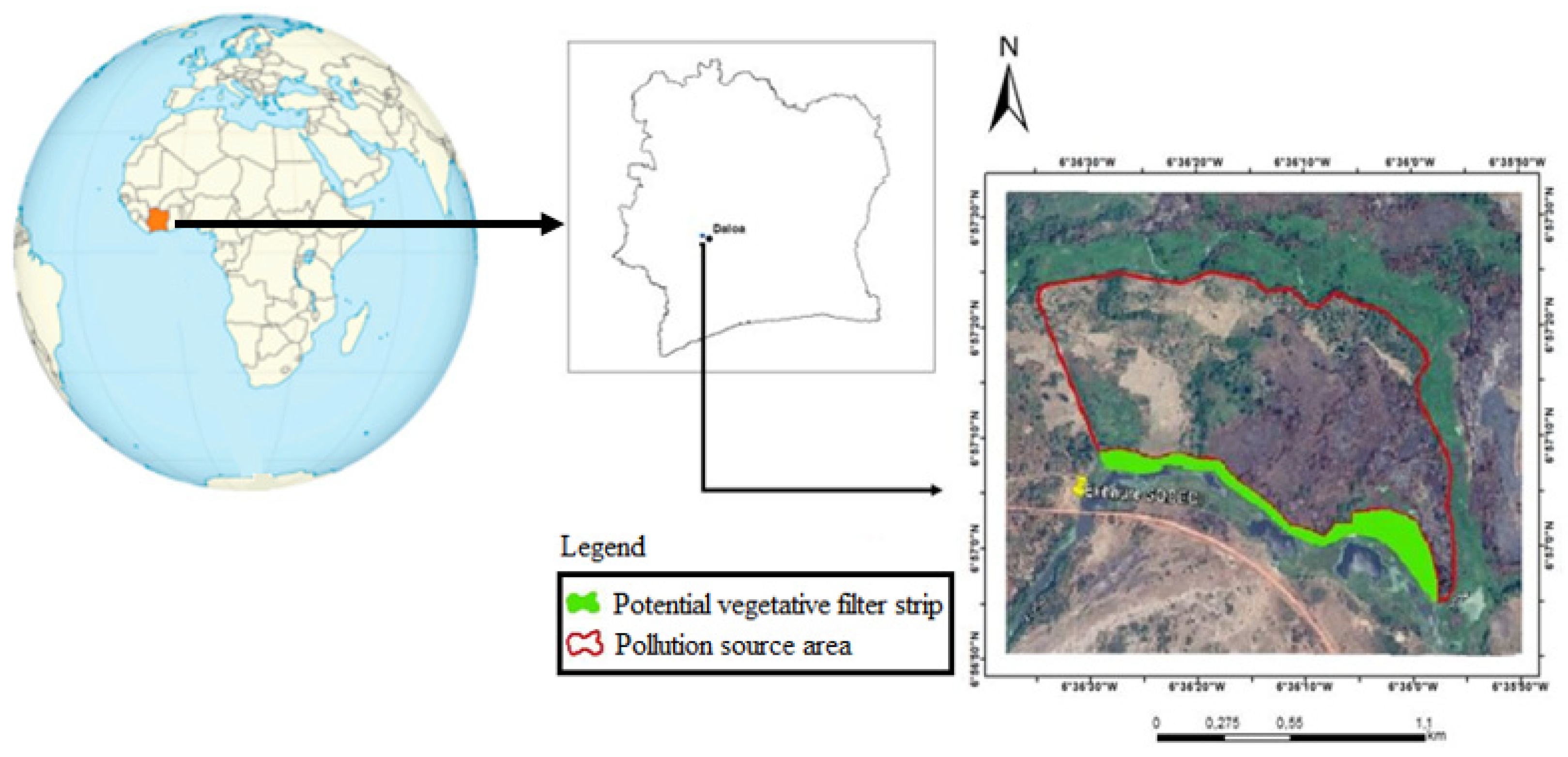
Figure 2.
Hydrographic network of the study site within the Lobo reservoir watershed.
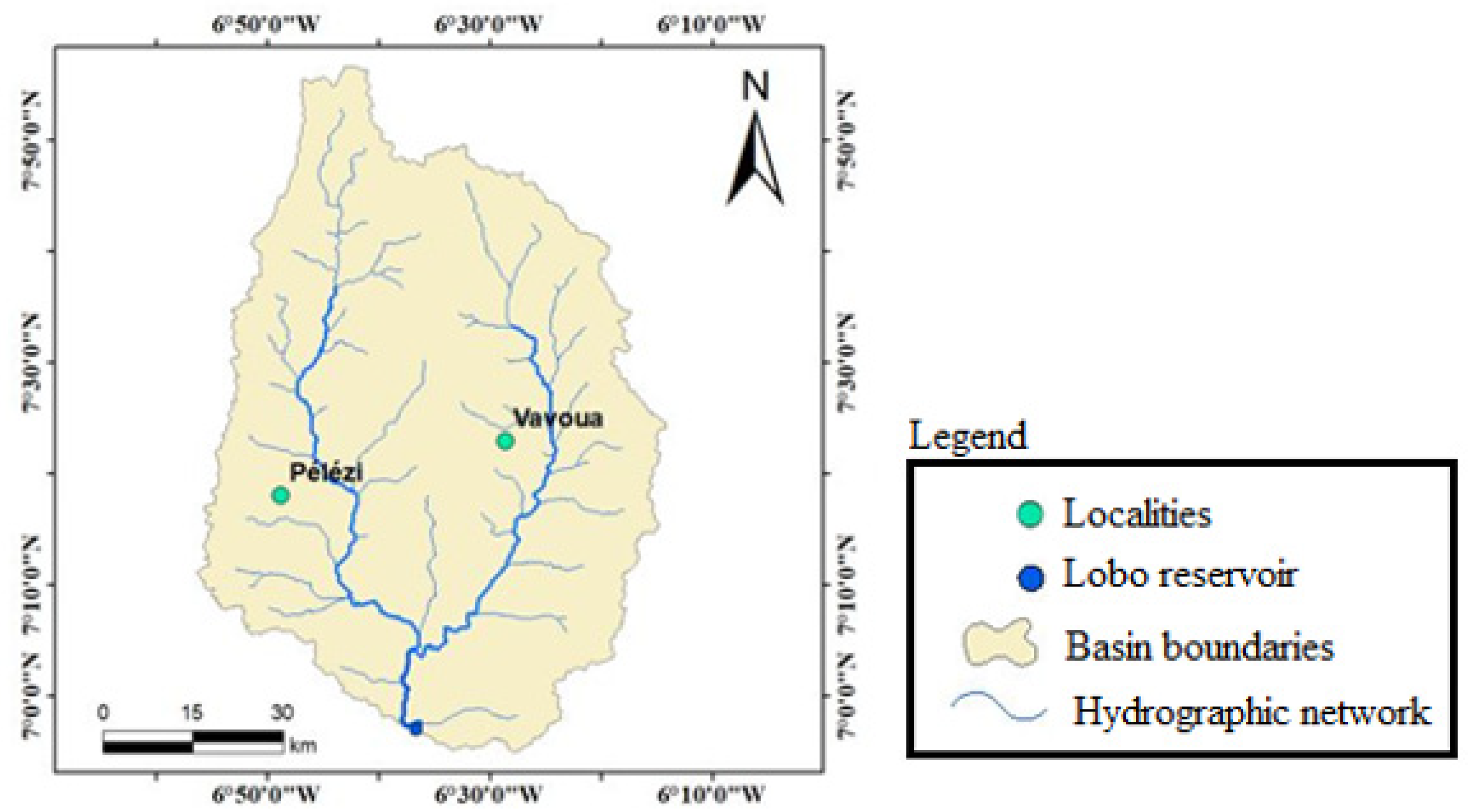
Figure 3.
Hydrograph of the rainy event studied.
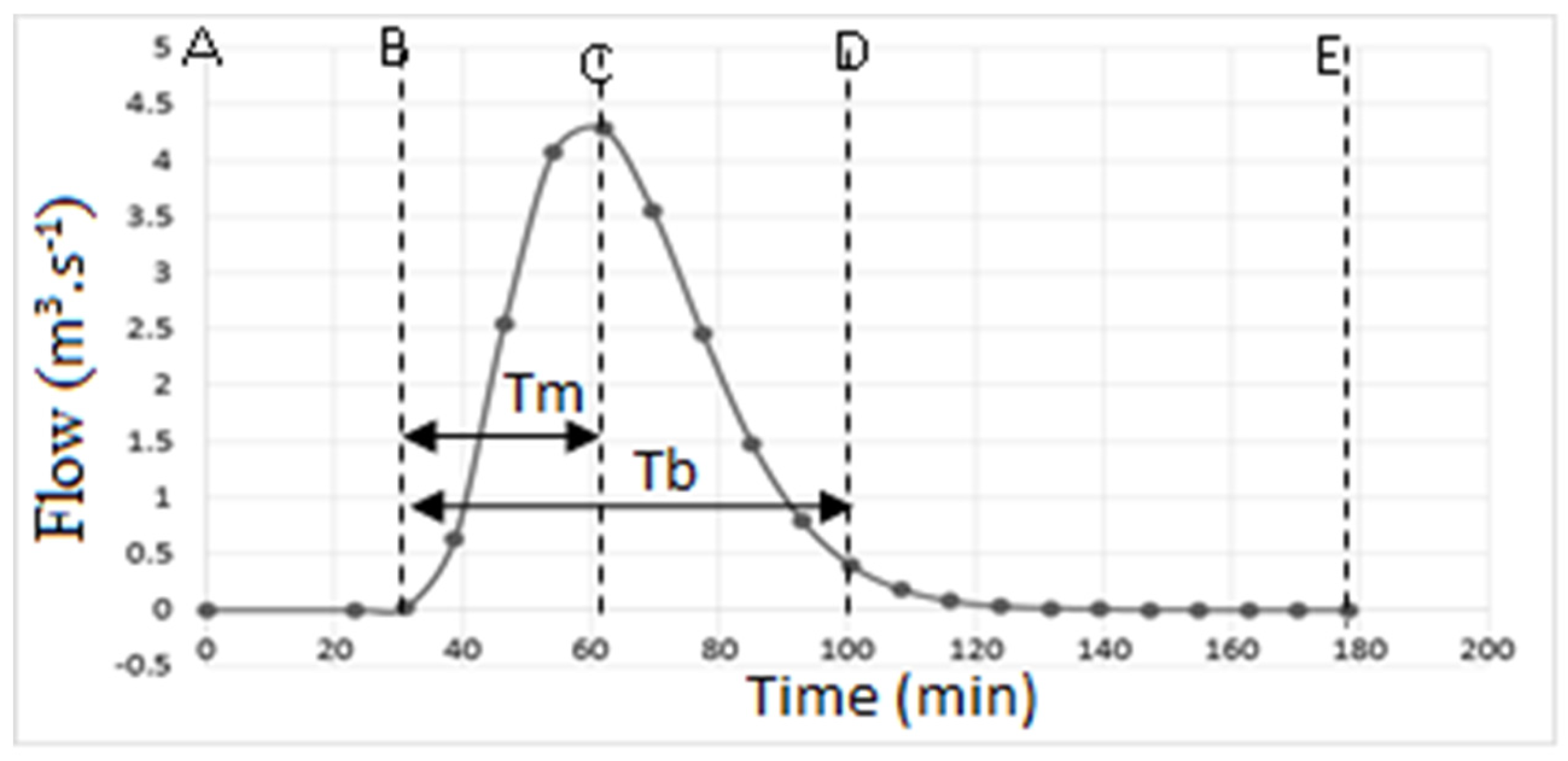
Figure 4.
Hyetogram of the contributing surface area.
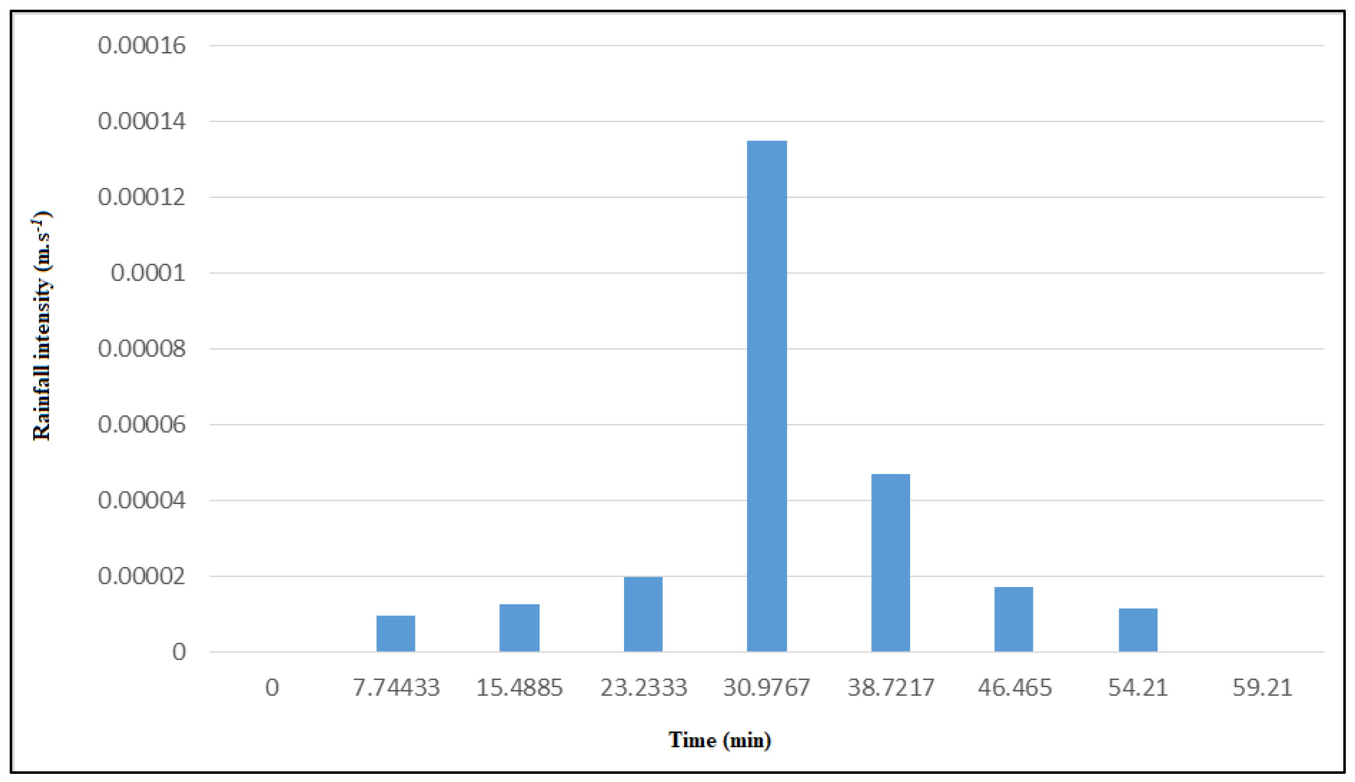
Figure 5.
Runoff reduction before simulation.
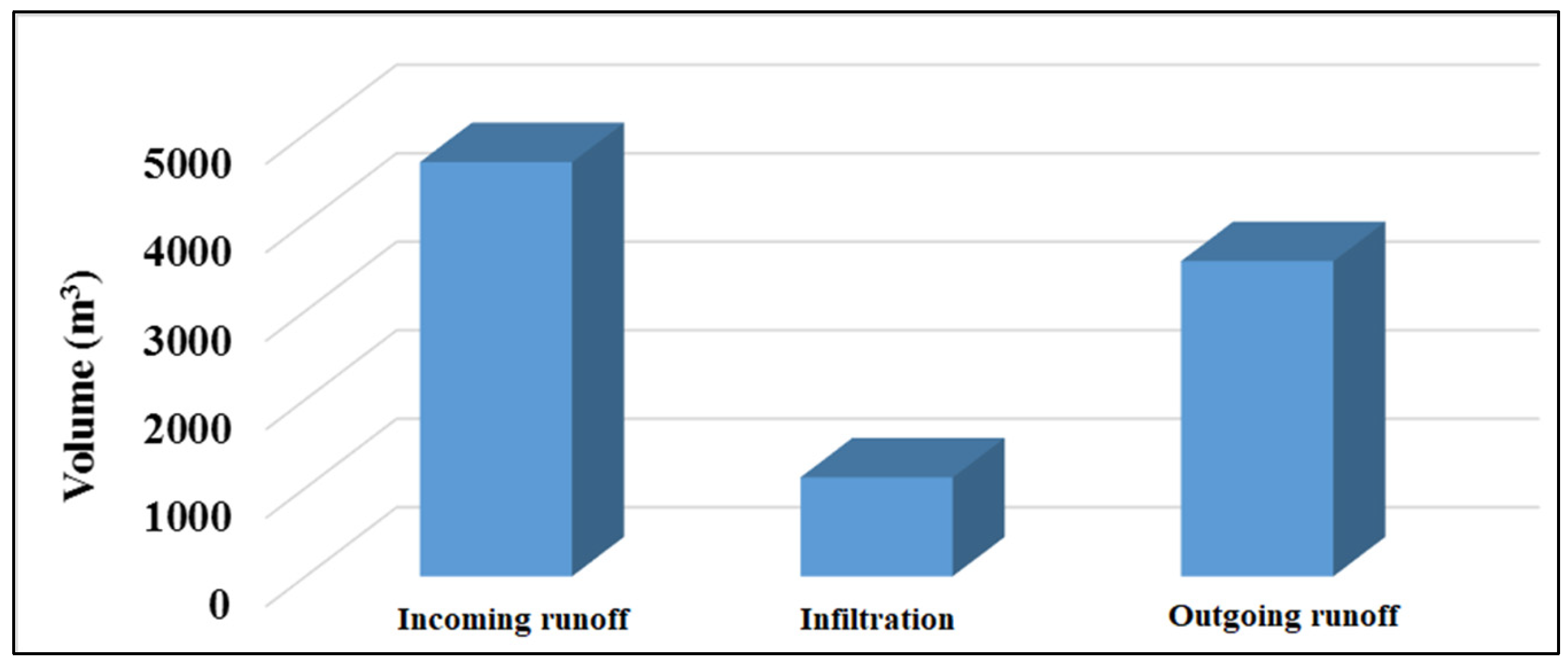
Figure 8.
Reduction of incoming flows and sediments after simulation under different scenarios.
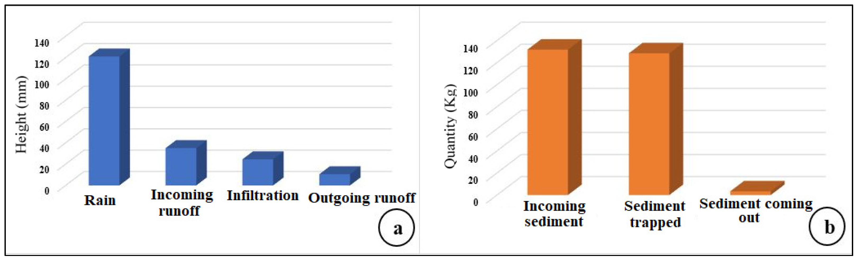

Table 1.
Potential optimal dimensions of the grass strip.
| Event | T1 | T2 | |
|---|---|---|---|
| Potential optimal dimensions | Width (m) | 12.70 | 22.95 |
| Length (m) | 300 | ||
Disclaimer/Publisher’s Note: The statements, opinions and data contained in all publications are solely those of the individual author(s) and contributor(s) and not of MDPI and/or the editor(s). MDPI and/or the editor(s) disclaim responsibility for any injury to people or property resulting from any ideas, methods, instructions or products referred to in the content. |
© 2024 by the authors. Licensee MDPI, Basel, Switzerland. This article is an open access article distributed under the terms and conditions of the Creative Commons Attribution (CC BY) license (http://creativecommons.org/licenses/by/4.0/).
Copyright: This open access article is published under a Creative Commons CC BY 4.0 license, which permit the free download, distribution, and reuse, provided that the author and preprint are cited in any reuse.


