Unraveling Electric Vehicle Preference: A Machine Learning Analysis of Vehicle Choice in Multi-Vehicle Households in the United States

1. Introduction

The United States, home to approximately 5% of the global population, is responsible for 28% of global carbon emissions, with the transportation sector contributing 27% (Zulinski, 2018). Since internal combustion engine vehicles (ICEV) powered by gasoline or diesel are significant contributors to carbon emissions in the transportation sector, it is imperative to augment the usage of vehicles that rely on alternative fuels such as electric vehicles (EVs). EVs include vehicles that are solely powered by electricity, such as battery electric vehicles (BEVs) (U.S. Department of Energy, 2013) or partially powered by electricity such as hybrid electric vehicles (HEVs) and plug-in hybrid electric vehicles (PHEVs) (Sen, 2010). By 2050, 50% of the global light-duty vehicle sector is likely to be made up of EVs, resulting in a 50% reduction in carbon emission levels from the sector (Ghandi and Paltsev, 2020). Understanding the usage pattern of EVs, therefore, lies at the heart of the endeavor to reduce carbon emissions.

EVs have garnered significant interest within the transportation research community. Well before their introduction to the market, researchers predicted the acceptance of EVs as a mode of transport. Several studies analyzing vehicle miles traveled (VMT) data from US households projected that EVs would be more suitable for multi-vehicle households, which were expected to be early adopters of this new technology (Musti and Kockelman, 2011; Sherman, 1980; Tamor and Milačić, 2015). With the introduction of EVs into the market, the projections proved to be accurate; the most recent National Household Travel Survey data (NHTS 2017) shows that majority of EV-owning households are multi-vehicle households (78.7% for HEVs, 83.4% for PHEVs and 92.7% for BEVs) (Li et al., 2019). Since multi-vehicle households represent the major portion of the EV market, it is essential to investigate the usage patterns of these households in relation to their EVs.

Although studies on the usage of EVs in multi-vehicle households with at least one ICEV and one EV are limited in number, they exist. Some recent studies have utilized GPS data to identify factors influencing EV usage and assess their potential for reducing greenhouse gas emissions (Chakraborty et al., 2022; Srinivasa Raghavan and Tal, 2021). Other studies have evaluated how EVs are used when replacing an ICEV in multi-vehicle households (Karlsson, 2020). To evaluate usage, these studies have collectively used metrics like VMT, VKT (vehicle kilometers traveled), utility factor (fraction of VMT electrified), and daily driving distance. Even fewer in number are studies that specifically explore vehicle choice in multi-vehicle households (with at least one EV and one ICEV). This choice holds significance because the use of EVs in multi-vehicle households has cascading effects on the gasoline VMT and carbon emissions from ICEVs (Srinivasa Raghavan and Tal, 2021). Furthermore, gaining a deeper understanding of this choice can assist policymakers in formulating policies based on the motivators and barriers of EV usage. Two European studies have modeled this choice by creating artificial multi-vehicle households (Bucher et al., 2020; Jensen and Mabit, 2015). However, the EV markets in those countries differ significantly from the US EV market. To the best of our knowledge, there have been no studies in the US that model vehicle choices for daily trips in such multi-vehicle households.

This study aims to expand research on vehicle choice in US multi-vehicle households, specifically those with at least one EV and one ICEV. It also addresses some limitations of previous studies on the same topic. Firstly, unlike previous studies, this research incorporates clustering analysis to capture the heterogeneity in trips. To highlight the significance of capturing heterogeneity in trips, consider the following example: Two trips covering the same distance might be regarded as different because they serve completely different purposes (Ozhegov and Ozhegova, 2019). Conversely, two trips with different distances might be considered similar due to other shared attributes. A clustering analysis would be able to capture this heterogeneity by grouping similar trips together based on a number of attributes (instead of only one attribute), something that a simple discrete-choice model fails to do. Secondly, this study utilizes the NHTS 2017 datasets, which provide information on multi-vehicle households in the US that naturally adopted EVs. Consequently, these households offer a more representative sample of the overall population. Thirdly, this study employs interpretable machine learning techniques to capture the non-linear relationships between explanatory variables and household vehicle choice. By doing so, it aims to address the complexity and intricacies of these relationships. With the aforementioned research gaps in mind, this study seeks to answer the following questions:

What type of trips are most likely to be made by EVs in US multi-vehicle households?

How do different socio-demographic and built-environment variables influence the choice of using EVs for individual trips in US multi-vehicle households?

The rest of the article is organized as follows. Section 2 (literature review) summarizes the articles and the findings that are relevant to the research questions of this study. Section 3 (data) provides a description of the dataset used in this study and the data preprocessing steps. Section 4 (methodology) section contains an overview of the models used in this study as well as the metrics used to evaluate and interpret them. The last two sections of the article are section 5 (Results and Discussion) and section 6 (Conclusion), which present this study's findings, implications, and concluding statements.

2. Literature Review

In the context of EVs, previous studies have explored a wide range of topics like vehicle market share (e.g., Vergis and Chen, 2014), user perceptions (e.g., Egbue and Long, 2012), incentives (e.g., Hardman et al., 2017). However, the literature review for this study mainly consists of studies that explored the adoption and usage of electric vehicles in the light-duty vehicle sector (Table 1). The oldest article in the review was from 1998 and the most recent one was from 2022.

2.1. Adoption

The vast majority of studies on EVs are related to “adoption” or the decision to purchase these vehicles. The studies falling under this category used discrete choice models to explore the adoption behavior and its determinants in the market with regard to EVs. These determinants can be broadly classified into four groups namely, demographic, contextual, situational, and psychological (Singh et al., 2020).

Before EVs became widely available in the market, studies relied upon stated preference surveys to explore adoption behavior of potential EV owners. These studies found fuel cost as one of the most important determinants of EV adoption. A study found that Americans were willing to pay $7600 more to own an EV (Tompkins et al., 1998) and American EV adoption was more sensitive to fuel cost reductions and charging availability than Japanese EV adoption (Tanaka et al., 2014). Among the US states, the fuel cost reduction had the greatest impact on consumers’ willingness to pay for EVs in California. In Germany, a stated preference study found that consumers’ willingness to pay was determined by factors such as fuel cost, emission reduction, tax exemptions (Hackbarth and Madlener, 2013). The results from a study in Ireland, which explored similar factors, showed that respondents place a higher utility on fuel cost reduction compared to tax exemption and emission reduction (Caulfield et al., 2010). Similar results were drawn from a systemic literature review study, which concluded that consumers state the cost components (fuel cost and purchase cost) as the most important determinant of adoption (Carlucci et al., 2018).

The more recent studies used revealed preference data to explore the determinants of EV adoption. Although these studies reiterate some of the findings from the stated preference surveys, they find a wider range of determinants. These determinants and their impact on EV adoption were found to vary widely across the different states in the US (Liu et al., 2019). Nevertheless, the results from the revealed preference studies suggest the use of a combination of social, economic, infrastructural and policy tools to increase EV adoption. Socio-economic determinants such as age, education, income, household size, number of vehicles in the household, marital status, and political affiliation were deemed significant in some studies (Shin et al., 2019). Infrastructural and policy factors such as publicly available charging stations, gasoline and electricity prices, HOV lane access, and the presence of purchase incentives were also found important determinants of EV market share (Vergis and Chen, 2014). A study exploring EV market share in different US states found that electricity price affects electric vehicle adoption rate the most (Soltani-Sobh et al., 2017).

2.2. Usage

Although it is important to understand the adoption of EVs, their impact on GHG emission reduction is determined by their usage patterns within the households that own them. With regard to EV usage, the existing studies (on single and multi-vehicle households) mostly explore determinants of EV usage by modeling vehicle miles travelled (VMT) or vehicle kilometers travelled (VKT). But there exists a shortage in the number of studies on vehicle choice in multi-vehicle households. The studies on EV usage that were reviewed for this study are presented in Table 1.

Before the availability of EVs in the market, several studies have assessed the potential acceptability of EVs in both single and multi-vehicle households. The studies used a combination of metrics (e.g., VMT, range, number of days daily driving distance exceeds EV range) and performed their assessments in different scenarios (e.g., gas cost $5 per gallon, gas cost $7 per gallon). Assessments from the studies lead to the conclusion that EVs are technically and economically better suited to multi-vehicle households (Booz and Hamilton, 1980; Jakobsson et al., 2016a; Musti and Kockelman, 2011; Tamor and Milačić, 2015). As compared to single vehicle household driving requirements, multi-vehicle household driving requirements supported the adoption of EVs with a lower range (Jakobsson et al., 2016a). Replacing one vehicle in a multi-vehicle instead of replacing the only vehicle in a single-vehicle household was expected to electrify roughly twice as many miles (Tamor and Milačić, 2015). More specifically, EVs were found to be better suited as the second car (the car with lower annual VMT) in multi-vehicle households because of the more frequent driving and shorter distances covered by these second cars (Jakobsson et al., 2016a).

Given the potential acceptability of EVs in multi-vehicle households, the researchers became interested in monitoring EV usage in such households. To study EV usage during the early adoption phase, some researchers provided an EV as a replacement for a ICEV in multi-vehicle households. They often found that the owners adapt their driving behavior (e.g., take alternative routes) to suit the new EV in their household (Jakobsson et al., 2022; Jakobsson et al., 2016). The studies collectively suggest that there exists a large heterogeneity in the EV driving patterns; some household drive their EVs more than the replaced car and some drive it less. Some recent studies, however, did not provide an EV as a replacement but collected data from EV owning households instead (Chakraborty et al., 2022; Mandev et al., 2022; Srinivasa Raghavan and Tal, 2021). They find that a range of factors can cause heterogeneity in EV driving patterns such as population density, attitudes towards technology and lifestyle preferences. These studies underscore the importance of charging infrastructure (especially the availability of level 2 charging at home) as a determinant of eVMT (Electrified Vehicle Miles Travelled) in multi-vehicle households. Moreover, PHEVs were found to have a higher total VMT and a higher share of household VMT compared to BEVs.

To the best of our knowledge, only two European studies have explored the vehicle choice in multi-vehicle households (with at least one electric and one internal combustion engine vehicle). A Danish study found that the number of trip legs, the drivetime, requirement to charge the vehicle all had negative effects on the probability of choosing EV. On the other hand, precipitation, urban area had positive effects on the choice (Jensen and Mabit, 2015). A study in Switzerland modeled household vehicle choice as a function of trip attributes, socio-demographic variables, and spatio-temporal variables. After a comparison of different vehicle choice models, they suggest that trip duration, trip distance, weekend (indicator) are some of the most important determinants, negatively influencing the choice. However, they conclude that the choice cannot be predicted easily by the features considered in the study.

Table 1. Reviewed Articles on Electric Vehicle usage (From 2015 to 2022).

Serial	Title (Year)	Data	Variables Considered	Method(s)	Key Findings
1	Modelling real choice between conventional ad electric cars for homebased journeys (2015)	Data from 667 Danish households	Journey time, driving time, number of trip legs, journey distance, at least one charge, windspeed, precipitation, Citroen dummy, number of driving licenses, city dummy, first week dummy.	Logit model	The number of trip legs, the drivetime, requirement to charge the vehicle all had negative effects on the choice of EV. While precipitation, urban area had positive effects on the choice.
2	Electric vehicles in multi-vehicle households (2015)	Data from 446 vehicles in the Puget Sound Region in Washington	Range, DRA (days requiring adaptation)/Threshold for inconvenience	Trip Counting, Analytic estimations	Electric vehicles of the same range if deployed as a second car in two vehicle households would be electrify roughly twice as many miles as the deployment into one car households (replacing their only vehicle).
3	Are multi-car households better suited for battery electric vehicles? – Driving patterns and economics in Sweden and Germany (2016)	German household survey data (from 6339 vehicles) and Swedish GPS data (from 700 vehicles)	VKT (vehicles kilometers traveled), DRA (days requiring adaptation), range, capital expenditure, operating expenditure	Extrapolation and economic analysis	From the economic analysis, it was also found that BEVs are best suited for multi-car households. Secondary household cars in these households are better suited to be replaced by a BEV.
4	How are driving patterns adjusted to the use of a battery electric vehicle in two-car households? (2016)	GPS data from 10 Swedish households	DRA (days requiring adaptation), annual VKT, daily driving distance	Extrapolation	For most households, the EV is driven more than the replaced car. There exists a large heterogeneity in the usage and adaptation among the households. The EVs mainly replace the 40-70 km trips of the replaced car.
5	What are the value and implications of two-car households for the electric car? (2017)	GPS logging data for both cars in 64 commuting Swedish two-car households	VKT(vehicles kilometers traveled), SOC (State of Charge), TCO (Total Cost of Ownership)	Mixed integer quadratically constrained programming (MIQCP)	Two-car households in Sweden could derive a value of $7000 from the flexibility of owning an EV. This is because they can drive more on electricity, which is cheaper, and rely on their internal combustion engine vehicles for longer trips.
6	Exploring Factors that Influence Individuals' Choice Between Internal Combustion Engine Cars and Electric Vehicles (2020)	A dataset of 129 Swiss drivers over a period of 1 year	weekday/weekend, temperature, precipitation, sex, age, number of cars in household, work status, household size, long-distance trip leg, duration of activity, trip duration, household income, hour of day, month of year	Random Forest and Logit Model	The duration, distance, weekday/weekend has a larger effect than household size, but these variables do not possess a high predictive power. This indicated that the range of the vehicles is not a deciding factor in this choice.
7	Utilization of battery-electric vehicles in two-car households: Empirical insights from Gothenburg Sweden (2020)	GPS data from 20 Swedish two-car households	Range, VKT (vehicles kilometers traveled), Flexibility Utilization Index	Ex-post analysis	The electric vehicles performed a major share of the below range driving during the weekends.
8	Electrification of Vehicle Miles Traveled and Fuel Consumption within the Household Context A Case Study from California, U.S.A. (2022)	A dataset of 650 vehicles from 287 Californian households	range, charging frequency, frequency of long-distance travel, frequency of overlaps, household VMT, ICEV mileage	Statistical Analysis and Regression	A short-range PHEV can electrify up to 70% of the eVMT of long-range BEVs (Bolt and Model S). Hence, PHEVs with 35-mile all-electric range can be used as tools to decarbonize the transport sector.
9	How do users adapt to a short-range battery electric vehicle in a two-car household? Results from a trial in Sweden (2022)	GPS data from 25 Swedish two-car households	DRA (days requiring adaptation), daily driving distance	Quantitative, qualitative, and mixed methods	There exists a large heterogeneity in driving adaptation and behavior; some households use the electric vehicle more than the replaced car; some use it less. Some households change their driving style when they use the electric vehicle.
10	Integrating plug-in electric vehicles (PEVs) into household fleets- factors influencing miles traveled by PEV owners in California (2022)	Survey data of 4125 Californian Households with BEVs or PHEVs	PEV characteristics, other household vehicle characteristics, built environment variables, household characteristics, respondent characteristics, other factors influencing PEV use	OLS Regression, SUR Model, Hypothesis Tests	eVMT is correlated with traditional factors such as population density, attitudes towards technology and lifestyle preferences. PEVs are driven as much as ICEVs. The availability of level 2 charging at home greatly influences the eVMT.

Table 1. Reviewed Articles on Electric Vehicle usage (From 2015 to 2022).

Serial	Title (Year)	Data	Variables Considered	Method(s)	Key Findings
1	Modelling real choice between conventional ad electric cars for homebased journeys (2015)	Data from 667 Danish households	Journey time, driving time, number of trip legs, journey distance, at least one charge, windspeed, precipitation, Citroen dummy, number of driving licenses, city dummy, first week dummy.	Logit model	The number of trip legs, the drivetime, requirement to charge the vehicle all had negative effects on the choice of EV. While precipitation, urban area had positive effects on the choice.
2	Electric vehicles in multi-vehicle households (2015)	Data from 446 vehicles in the Puget Sound Region in Washington	Range, DRA (days requiring adaptation)/Threshold for inconvenience	Trip Counting, Analytic estimations	Electric vehicles of the same range if deployed as a second car in two vehicle households would be electrify roughly twice as many miles as the deployment into one car households (replacing their only vehicle).
3	Are multi-car households better suited for battery electric vehicles? – Driving patterns and economics in Sweden and Germany (2016)	German household survey data (from 6339 vehicles) and Swedish GPS data (from 700 vehicles)	VKT (vehicles kilometers traveled), DRA (days requiring adaptation), range, capital expenditure, operating expenditure	Extrapolation and economic analysis	From the economic analysis, it was also found that BEVs are best suited for multi-car households. Secondary household cars in these households are better suited to be replaced by a BEV.
4	How are driving patterns adjusted to the use of a battery electric vehicle in two-car households? (2016)	GPS data from 10 Swedish households	DRA (days requiring adaptation), annual VKT, daily driving distance	Extrapolation	For most households, the EV is driven more than the replaced car. There exists a large heterogeneity in the usage and adaptation among the households. The EVs mainly replace the 40-70 km trips of the replaced car.
5	What are the value and implications of two-car households for the electric car? (2017)	GPS logging data for both cars in 64 commuting Swedish two-car households	VKT(vehicles kilometers traveled), SOC (State of Charge), TCO (Total Cost of Ownership)	Mixed integer quadratically constrained programming (MIQCP)	Two-car households in Sweden could derive a value of $7000 from the flexibility of owning an EV. This is because they can drive more on electricity, which is cheaper, and rely on their internal combustion engine vehicles for longer trips.
6	Exploring Factors that Influence Individuals' Choice Between Internal Combustion Engine Cars and Electric Vehicles (2020)	A dataset of 129 Swiss drivers over a period of 1 year	weekday/weekend, temperature, precipitation, sex, age, number of cars in household, work status, household size, long-distance trip leg, duration of activity, trip duration, household income, hour of day, month of year	Random Forest and Logit Model	The duration, distance, weekday/weekend has a larger effect than household size, but these variables do not possess a high predictive power. This indicated that the range of the vehicles is not a deciding factor in this choice.
7	Utilization of battery-electric vehicles in two-car households: Empirical insights from Gothenburg Sweden (2020)	GPS data from 20 Swedish two-car households	Range, VKT (vehicles kilometers traveled), Flexibility Utilization Index	Ex-post analysis	The electric vehicles performed a major share of the below range driving during the weekends.
8	Electrification of Vehicle Miles Traveled and Fuel Consumption within the Household Context A Case Study from California, U.S.A. (2022)	A dataset of 650 vehicles from 287 Californian households	range, charging frequency, frequency of long-distance travel, frequency of overlaps, household VMT, ICEV mileage	Statistical Analysis and Regression	A short-range PHEV can electrify up to 70% of the eVMT of long-range BEVs (Bolt and Model S). Hence, PHEVs with 35-mile all-electric range can be used as tools to decarbonize the transport sector.
9	How do users adapt to a short-range battery electric vehicle in a two-car household? Results from a trial in Sweden (2022)	GPS data from 25 Swedish two-car households	DRA (days requiring adaptation), daily driving distance	Quantitative, qualitative, and mixed methods	There exists a large heterogeneity in driving adaptation and behavior; some households use the electric vehicle more than the replaced car; some use it less. Some households change their driving style when they use the electric vehicle.
10	Integrating plug-in electric vehicles (PEVs) into household fleets- factors influencing miles traveled by PEV owners in California (2022)	Survey data of 4125 Californian Households with BEVs or PHEVs	PEV characteristics, other household vehicle characteristics, built environment variables, household characteristics, respondent characteristics, other factors influencing PEV use	OLS Regression, SUR Model, Hypothesis Tests	eVMT is correlated with traditional factors such as population density, attitudes towards technology and lifestyle preferences. PEVs are driven as much as ICEVs. The availability of level 2 charging at home greatly influences the eVMT.

2.3. Summary

From the literature review, it was observed that studies on the vehicle choice within multi-vehicle households with an EV and a ICEV are rarely found in the US. The studies that did explore this topic were conducted in two European markets (Denmark and Switzerland), where the driving needs are very different from those in the US. The studies were limited in certain aspects. Firstly, the households considered in the existing studies may not be representative of the broader population of multi-vehicle households adopting EVs . This is due to the fact that the household samples in these studies did not previously own EVs and were provided with one solely for research purposes. Secondly, although Bucher et al. (2020) hinted at the existence of non-linear effects of explanatory variables on vehicle choice, none of the studies reported or discussed these effects. Thirdly, the studies on this topic incorporated trip attributes in their models, but they considered these attributes in isolation. This approach introduces bias in the results since it fails to capture the heterogeneity in trips, as highlighted by Ozhegov and Ozhegova (2019). It is important to recognize that a trip's similarity or dissimilarity to another trip is based on multiple attributes rather than just a single attribute. This study fulfills the research gaps by modeling the vehicle choice of a representative sample of multi-vehicle households and employing machine learning techniques that capture the heterogeneity in trips and the non-linear effects of variables on vehicle choice.

3. Data

3.1. NHTS 2017

This study uses the 2017 National Household Travel Survey (NHTS) datasets, which contain travel information for US residents in all 50 states and the District of Columbia (U.S. Department of Transportation, 2017). These surveys employ professional processing procedures (e.g., weighted response rates to account for disproportionate sampling across a region) to capture travel behavior and its seasonal variation over 12 months (Liu et al., 2019; U.S. Department of Transportation, 2017). The 2017 NHTS consists of 4 datasets namely, household, vehicle, person, and trip datasets.

3.2. Data Cleaning

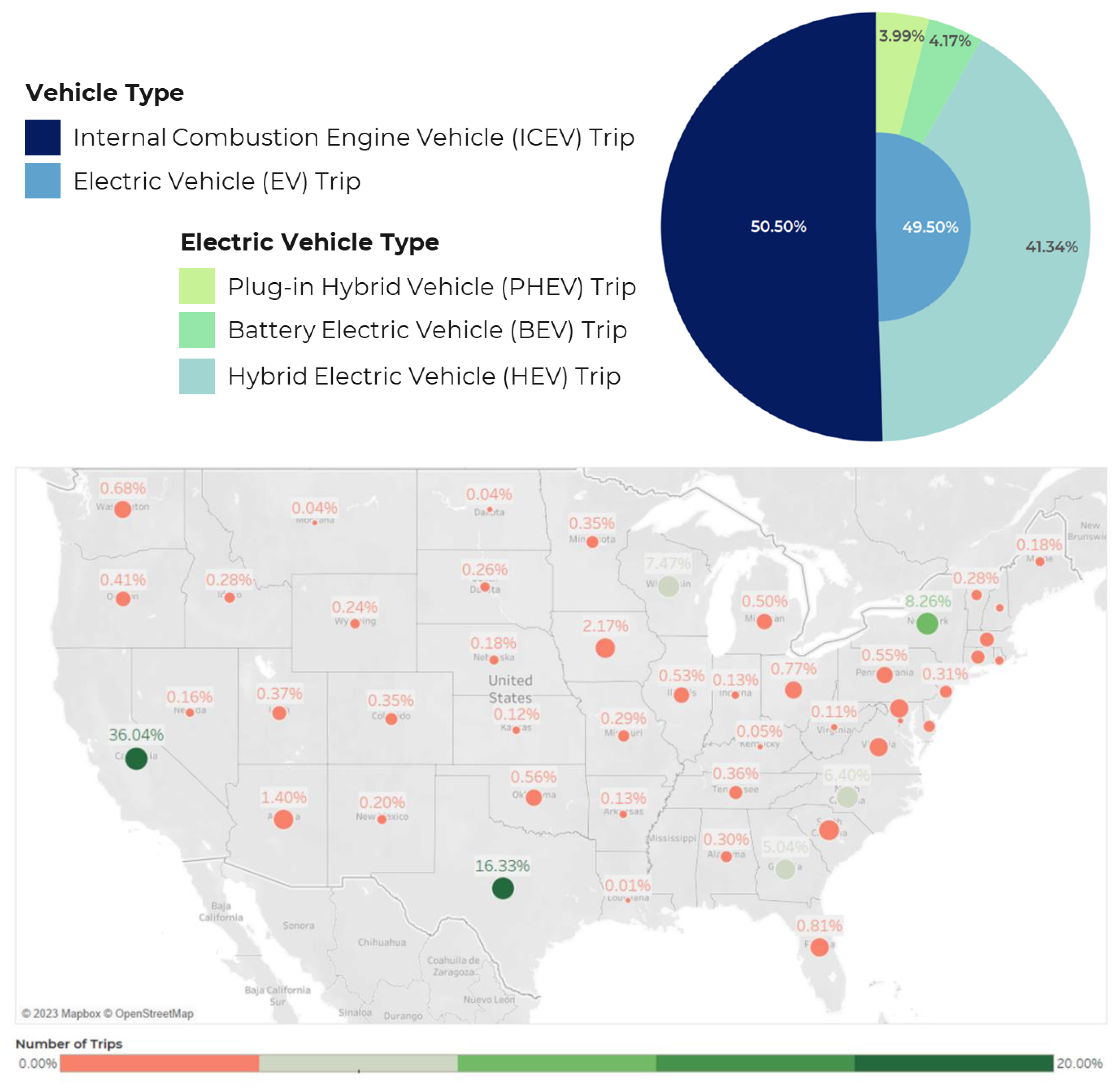
The NHTS trip dataset is an inventory of all trips taken within a specified 24-hour period by household members older than 5. It contains 923,572 trips made by 117,222 households. Among them, 81,913 (69.88% of all households) households owned multiple vehicles. They made a total of 589,750 trips (63.86% of all trips). The trip data for the multi-vehicle households were merged with the vehicle and person datasets to retrieve the vehicle, household, and driver attributes. This study deals with households owning at least one ICEV and at least one EV. Hence, trips made by households owning only EVs or only ICEVs were taken out. As this study is only interested in the household vehicle choice for a trip from their vehicle holdings, trips involving non-household vehicles were discarded. Observations with missing/unknown values for important variables were also taken out. To drop observations with excessive average trip speeds (e.g., 1495 mph) (derived from trip distance and duration), the top speed of the fastest model for each vehicle manufacturer was checked (Perez, 2020). Lastly, observations with return trips (trips where the destination is home) were excluded. This data cleaning step is justified because household members are bound to use the vehicle for return trips that they chose when leaving home. Since there is not vehicle choice involved for these trips, they were not considered in this study. The cleaned dataset contained a total of 19,825 trips made by 3917 households. Figure 1 (top) shows the proportion of EV trips and ICEV trips in the dataset. It can be observed that the cleaned dataset is balanced with regard to the proportion of EV trips (49.5%) and ICEV trips (50.5%), which is conducive to the performance of machine learning models (Jia, 2019). Among the EV trips, most of the trips were made by HEVs. Figure 1 (bottom) also contains a symbol map showing the spatial distribution of trips across the different states. The cleaned dataset contains trips from 49 states (except Mississippi) and the district of Columbia. Major shares of the trips are from the states highlighted with green and light green symbols (California, Texas, New York, Wisconsin, North Carolina, and Georgia).

Figure 1. The percentages of trips made by different vehicle types and fuel types (top) and number of trips from 50 states in the US (bottom).

Figure 1. The percentages of trips made by different vehicle types and fuel types (top) and number of trips from 50 states in the US (bottom).

3.3. Variable Selection

The variable selection for this study was informed by existing studies on EVs and multicollinearity assessment. Since the study intends to identify the type of trips that are most likely to be made by EVs in multi-vehicle households, individual trip attributes (e.g., trip purpose, trip distance, number of passengers) were considered in the modeling framework. Trip attributes have been previously used in studies that modeled EV usage (Bucher et al., 2020; Jensen and Mabit, 2015). Based on these studies a number of trip attributes were considered to be included in the model. In addition to trip attributes, the models also included household attributes which have been commonly linked to EV usage and adoption (Chakraborty et al., 2022; Jia, 2019; Liu et al., 2019; Shin et al., 2019). Existing EV studies also identified the effects of person attributes (Bucher et al., 2020; Caulfield et al., 2010; Li et al., 2019; Tompkins et al., 1998), built-environment variables (Musti and Kockelman, 2011; Vergis and Chen, 2014) and gas price (De Borger et al., 2016). Based on previous studies, an initial list of variables was produced. Some of these variables had multi-collinearity, which were excluded from the list. The final subset of variables selected for modeling had VIFs below 4. Table 2 shows the variables which were included in the final modeling framework and their descriptive statistics.

Table 2. The descriptive statistics of the variables used in this study.

	Variable		Categories	Distribution
Household Attributes	Home Ownership (Binary)		Rent's a House	91.26%
			Own's a House	8.74%
	Household Income (Discrete)		Low (<$50,000)	9.73%
			Medium ($50,000 - $150,000)	57.24%
			High (>$150,000)	33.03%
	Number of Household Workers (Discrete)		0	17.53%
			1	25.61%
			2	45.92%
			3	8.49%
			4	2.12%
			5	0.33%
	Children (Binary)		No children	90.42%
			1 or more children	9.58%
Driver Attributes	Driver's Age (continuous)		-	52.49 ± 15.65*
	Driver's Education Level (Discrete)		No high school degree	8.64%
			High school or associate degree	19.31%
			Bachelor's degree or higher	72.06%
	Driver's Sex (Binary)		Female	43.54%
			Male	56.46%
Built Environment Variables	Employment Density in Workers Per 0.01 Square Miles (Continuous)		-	3.74 ± 4.52*
	Population Density in Persons Per 0.01 Square Miles (Continuous)		-	1.54 ± 1.52*
**Trip Day Gas Price in cents per gallon (Continuous)			-	246.86 ± 25.64*
Trip Attributes		Weekday/Weekend (Binary)	Weekday	77.42%
			Weekend	22.58%
		Starting Time (Discrete)	12 AM - 6 AM	2.53%
			6 AM - 10AM	30.06%
			10 AM - 3 PM	38.06%
			3 PM - 7 PM	24.44%
			7 PM - 12 AM	4.9%
		Home/Non-home Based (Binary)	Home-based trip	49.42%
			non-home-based trip	50.58%
		Trip Purpose (Discrete)	Errands	16.01%
			Others	10.41%
			Shopping or Dining	38.28%
			Social or recreational	14.81%
			Work	20.49%
		Dwelling time (Discrete)	1-15 minutes	29.31%
			15-50 minutes	24.04%
			50-150 minutes	25.08%
			More than 150 minutes	21.57%
		Trip Distance (Discrete)	0-2 miles	27.82%
			2-5 miles	28.41%
			5-15 miles	27.35%
			More than 15 miles	16.41%
		Number of Passengers (Discrete)	1 passenger	56.92%
			2-4 passengers	41.42%
			5 - 10 passengers	1.66%

Note: The distributions of continuous variables are presented as mean ± standard deviation. ** Note: The NHTS 2017 contains gas price data on the Petroleum Administration for Defense District (PADD) level.

Table 2. The descriptive statistics of the variables used in this study.

	Variable		Categories	Distribution
Household Attributes	Home Ownership (Binary)		Rent's a House	91.26%
			Own's a House	8.74%
	Household Income (Discrete)		Low (<$50,000)	9.73%
			Medium ($50,000 - $150,000)	57.24%
			High (>$150,000)	33.03%
	Number of Household Workers (Discrete)		0	17.53%
			1	25.61%
			2	45.92%
			3	8.49%
			4	2.12%
			5	0.33%
	Children (Binary)		No children	90.42%
			1 or more children	9.58%
Driver Attributes	Driver's Age (continuous)		-	52.49 ± 15.65*
	Driver's Education Level (Discrete)		No high school degree	8.64%
			High school or associate degree	19.31%
			Bachelor's degree or higher	72.06%
	Driver's Sex (Binary)		Female	43.54%
			Male	56.46%
Built Environment Variables	Employment Density in Workers Per 0.01 Square Miles (Continuous)		-	3.74 ± 4.52*
	Population Density in Persons Per 0.01 Square Miles (Continuous)		-	1.54 ± 1.52*
**Trip Day Gas Price in cents per gallon (Continuous)			-	246.86 ± 25.64*
Trip Attributes		Weekday/Weekend (Binary)	Weekday	77.42%
			Weekend	22.58%
		Starting Time (Discrete)	12 AM - 6 AM	2.53%
			6 AM - 10AM	30.06%
			10 AM - 3 PM	38.06%
			3 PM - 7 PM	24.44%
			7 PM - 12 AM	4.9%
		Home/Non-home Based (Binary)	Home-based trip	49.42%
			non-home-based trip	50.58%
		Trip Purpose (Discrete)	Errands	16.01%
			Others	10.41%
			Shopping or Dining	38.28%
			Social or recreational	14.81%
			Work	20.49%
		Dwelling time (Discrete)	1-15 minutes	29.31%
			15-50 minutes	24.04%
			50-150 minutes	25.08%
			More than 150 minutes	21.57%
		Trip Distance (Discrete)	0-2 miles	27.82%
			2-5 miles	28.41%
			5-15 miles	27.35%
			More than 15 miles	16.41%
		Number of Passengers (Discrete)	1 passenger	56.92%
			2-4 passengers	41.42%
			5 - 10 passengers	1.66%

Note: The distributions of continuous variables are presented as mean ± standard deviation. ** Note: The NHTS 2017 contains gas price data on the Petroleum Administration for Defense District (PADD) level.

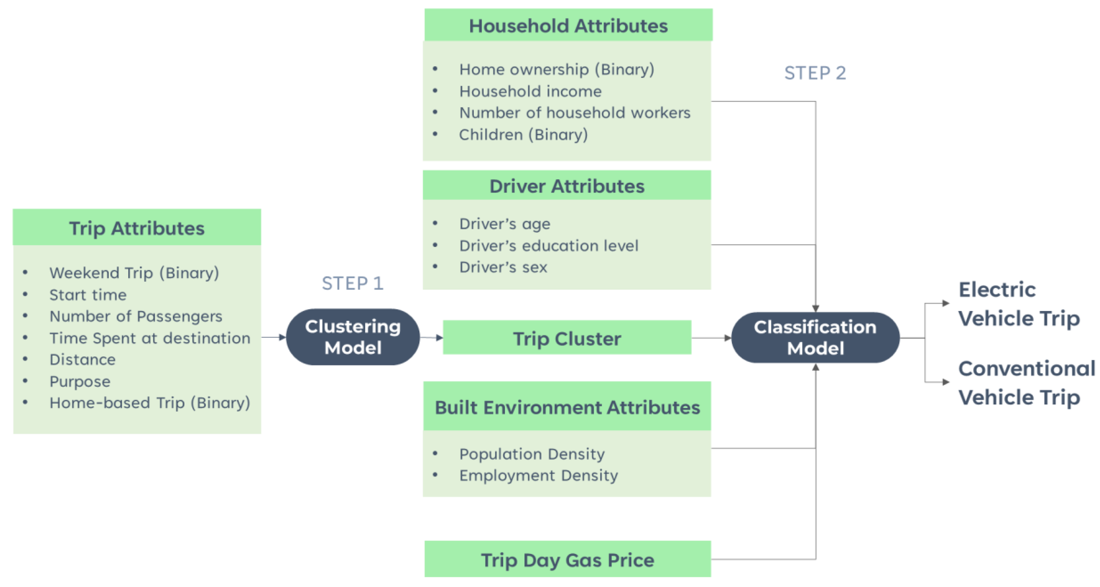
4. Methodology

This study used a combination of two machine-learning techniques to model household vehicle choice (Figure 2). The first model (clustering model) captured the heterogeneity in trips by clustering them based on trip attributes. The second model (classification model) predicted vehicle choice. It was hypothesized that individuals in multi-vehicle households make a choice between their electric and internal combustion engine vehicles based on the type of trip they are making. Hence, the classification model accepted the trip cluster from the clustering model as an input variable. In addition, the classification model also captured the effects of household attributes, driver attributes, gas price and built-environment variables by accepting them as inputs. The following subsections describe the two models in detail.

Figure 2. Two-step modeling framework used to predict vehicle choice.

Figure 2. Two-step modeling framework used to predict vehicle choice.

4.1. Clustering Model

Since these trips can vary based on a number of attributes (e.g., trip distance, starting time, trip purpose), a k-modes clustering analysis (Huang, 1998) was performed to cluster the trips. The clustering analysis maximized the homogeneity within the same trip cluster and minimized the homogeneity between different trip clusters. The trips were clustered based on seven attributes namely, weekend/weekday trip, starting time, number of passengers, dwelling time at destination, distance, trip purpose, home-based/non-home-based trip. The k-modes clustering approach, used in this study, is less vulnerable to the local optima compared to statistical approaches such as the latent class analysis (Chaturvedi et al., 2001). K-modes clustering was chosen over k-means clustering because some of the variables of interest were unordered categorical variables (e.g., trip purpose, home-based/non-home-based trip). The continuous variables of interest (e.g., dwelling time at destination, trip distance) were converted into categorical variables before applying the k-modes clustering analysis. Although k-prototype clustering may make more sense for mixed data (with categorical and continuous variables), the k-modes clustering approach was found to provide clearer delineation among clusters for this specific dataset. Apart from the delineation among clusters, the model results are easier to interpret when the variable types are the same. Hence, the k-modes clustering was chosen over other the k-prototype clustering approach.

The k-modes clustering analysis in this study consisted of the following steps:

(1)

A set of observations from the dataset Q = [Q₁, Q₂, Q₃ ….. Q_k] is initialized as the cluster centroids using a density-based initialization algorithm (Cao et al., 2009). This initialization method helps avoid the necessity of running the algorithm multiple times to search for an effective solution. The observation with the maximum density is initialized as the first centroid. The remaining centroids are initialized based on density as well as the distance from other centroids.

(2)

Every trip/observation (denoted by X) outside Q, is assigned to a cluster from Q whose centroid had the smallest hamming distance (Pandit and Gupta, 2011) from X. Hamming distance can be defined as follows:

$$d\left(X,Q\right)=\sum _{j=1}^J\delta (x_j,q_j)\mathrm{where}\delta (x_j,q_j)=\left\{\begin{array}{c}0(x_j=q_j)\\ 1(x_j\ne q_j)\end{array}\right.$$

(3)

After every trip is assigned to a cluster, the cluster centroids in Q are updated based on the newly assigned trips. The hamming distances for each trip are recalculated and trips are assigned to new clusters based on the newly calculated hamming distances.

(4)

Step 3 is repeated until no trip in the dataset changes clusters. And the cost or the sum of the hamming distances for all the observations were recorded for the model with k clusters.

Models with clusters ranging from 2 to 10 were assessed. To assist the selection of the final clustering model, the elbow plot, the Silhouette Score (Rousseeuw, 1987) and cluster separation were evaluated. Moreover, the trip attributes for different clusters were observed. The model that provided the best scores for the evaluation metrics and a clear delineation among the clusters was selected as the final model.

4.2. Classification Model

Household vehicle choice (ICEV or EV) was modeled as a function of trip cluster (from the clustering model), household attributes, driver attributes, built-environment attributes, trip-day gas price. To accomplish this, 4 different modeling techniques were tested and compared. The first three models were tree-based machine learning models (decision tree, random forest, extreme gradient boosting). These models were chosen as candidate models because previous studies have found tree-based machine learning models to be highly accurate in predicting mode choice (Kim, 2021; Zhao et al., 2020). The last one among the four models was a logit model, which has been the most popular method applied to mode choice modeling. In order to generate training and testing subsets for the models, the cleaned dataset underwent random shuffling, followed by a split of 85% for training and 15% for testing purposes. The four modeling approaches were then compared based on cross-validation accuracy (10 fold cross-validation) (Zhao et al., 2020) and testing accuracy. Assessment of both cross-validation and testing accuracies ensures the maximum generalizability of the models. The most accurate model was then chosen to draw interpretations. The following sections provide a general overview of the four modeling techniques and the specific configurations used for this study.

4.2.1. Decision Tree

A decision tree performs classification by recursively partitioning the dataset based on its features (Myles et al., 2004). These partitions are also called “decisions”. The decision tree model takes a series of consecutive decisions to form a tree structure, which lead to its final predictions. For this study, a decision tree was implemented using the “DecisionTreeClassifier” class in python’s scikit-learn library. This class implements the CART version of the decision tree introduced by (Breiman, 1984). The mathematical formulation can be described as follows:

Given training vectors x_i ∈ R, i =1,2,3….l and a label vector y ∈ R^l, a decision tree performs partitioning such that observations with the same labels fall in the same group. The data at node m is represented by Q_m where the number of observations is n_m. For each candidate split, Ɵ=(j, t_m) consisting of a feature j and a threshold value t, the data is split into Q_m^left(Ɵ) and Q_m^right(Ɵ) subsets such that,

$$Q_m^{left}\left(\theta \right)=\left\{\left(x,y\right)|x_j<t_m\right\}$$

$$Q_m^{right}\left(\theta \right)=Q_m\backslash Q_m^{left}\left(\theta \right)$$

After a split is performed, the quality of the split is assessed based on the gini impurity function and the candidate split which provides the minimum impurity is selected as the final split for node m. In this way, subsets Q_m^left(Ɵ) and Q_m^right(Ɵ) are recursively produced until n_m=1. Since the set of features considered in this study consist of categorical features, they were converted into dummy variables as suggested by Breiman (2001).

4.2.2. Random Forest

A random forest is an ensemble technique that is applied to decision trees to improve generalization (improve the prediction accuracy for unseen data) (Myles et al., 2004). The technique is referred to as random forest because it combines a number of randomized decision trees (Biau and Scornet, 2016). The “RandomForestClassifier” class in python’s scikit-learn library was used to implement the random forest model in this study. The class implements the version of random forests introduced by Breiman (2001). The random forest algorithm for this study and the hyperparameters involved in each step are discussed below:

(1)

At first a subset of the data is formed by bootstrapping (Breiman, 1996). In this step, a random sample of the data is drawn with replacement. This implies that some observations may be duplicated, and others may be left out of the sample.

(2)

Next, a decision tree is constructed using the bootstrapped sample and a set of randomly selected features. As recommended by previous studies (Liaw and Wiener, 2002), the number of randomly selected features was set as the square root of the total number of features rounded to the nearest integer. The decision tree is grown until the number of observations at a node reaches 1.

(3)

The number of decision trees to be grown was set to 1000; the first two steps were repeated 1000 times.

(4)

To make a prediction for a new observation, each decision tree in the forest is traversed and the predictions from each tree are recorded. Finally, the majority vote of predictions is taken as the final prediction.

4.2.3. Extreme Gradient Boosting

Extreme Gradient Boosting model (XG Boost) is another ensemble technique applied to decision trees which is based on the gradient boosting model (Friedman, 2001). It grows a sequence of decision trees with low depth and each tree is trained by putting more weight on the incorrect predictions of the preceding trees (Chen and Guestrin, 2016). The technique minimizes a loss function using gradient descent. It works by iteratively adding decision trees to the model, with each new tree attempting to correct the errors made by the previous trees. At each iteration, the algorithm calculates the gradient and the hessian of the loss function with respect to the current model and uses this information to create a new decision tree that minimizes the loss function. The gradient and hessian are used to split the data into regions, with each region corresponding to a specific leaf node in the decision tree. The algorithm assigns weights to each region based on the objective function and the current model and uses these weights to make predictions. The XGBoost package in python was used to implement the model.

4.2.4. Binary Logit

This study also employed a binary logit model, which served as a baseline for comparison. The binary logit has been applied in a wide number of studies to model mode choice (Bhat, 1997; Yang et al., 2018). The dependent variable of the model Y_i could take either of the values 1 (for EV) or 0 (for ICEV). The probability that the dependent variable equals 1 for an observation i is given by:

$$\mathrm{Pr}(Y_i=1\left|X_i\right)=\mathrm{e}\mathrm{x}\mathrm{p}\left(X_i\beta \right)/(1+\mathrm{e}\mathrm{x}\mathrm{p}(X_i\beta \left)\right)$$

(3)

X_i is a matrix of features; $\beta$ is a vector of unknown coefficients estimated via maximum likelihood estimation (MLE) on Stata 16. Robust standard errors were used in the process to account for possible heteroskedasticity (Cameron and Trivedi, 2010). The base case in this model (Kim and Gudmundur F. Ulfarsson, 2004) was the mode choice alternative ICEV.

4.2.5. Classification Model Interpretation

Although machine learning models have been widely successful in terms of their predictive accuracy, they have been criticized for the lack of interpretability compared to traditional discrete choice models such as the binary logit. However, some recent studies have utilized a number of interpretation methods to make machine learning models interpretable (Kim, 2021; Wang and Ross, 2018). Two such methods were used to interpret the best performing classification model. Firstly, the impurity-based variable importance of the predictors were estimated using the gini index (Zhao et al., 2020). This metric provided a measure of the predictive powers of the variables in the model. In addition, the accumulated local effects (ALE) (Apley and Zhu, 2020) were estimated to decipher the marginal effects of the independent variables on EV choice. ALE plots are able to illustrate any type of relationship (e.g., linear, multi-linear, non-linear) between a variable and the predicted outcome.

5. Results and Discussion

This section discusses the results from each of the two steps in the modeling framework. For each step, different model specifications are compared, and interpretations are drawn from the best model.

5.1. Clustering Model

5.1.1. Model Comparison

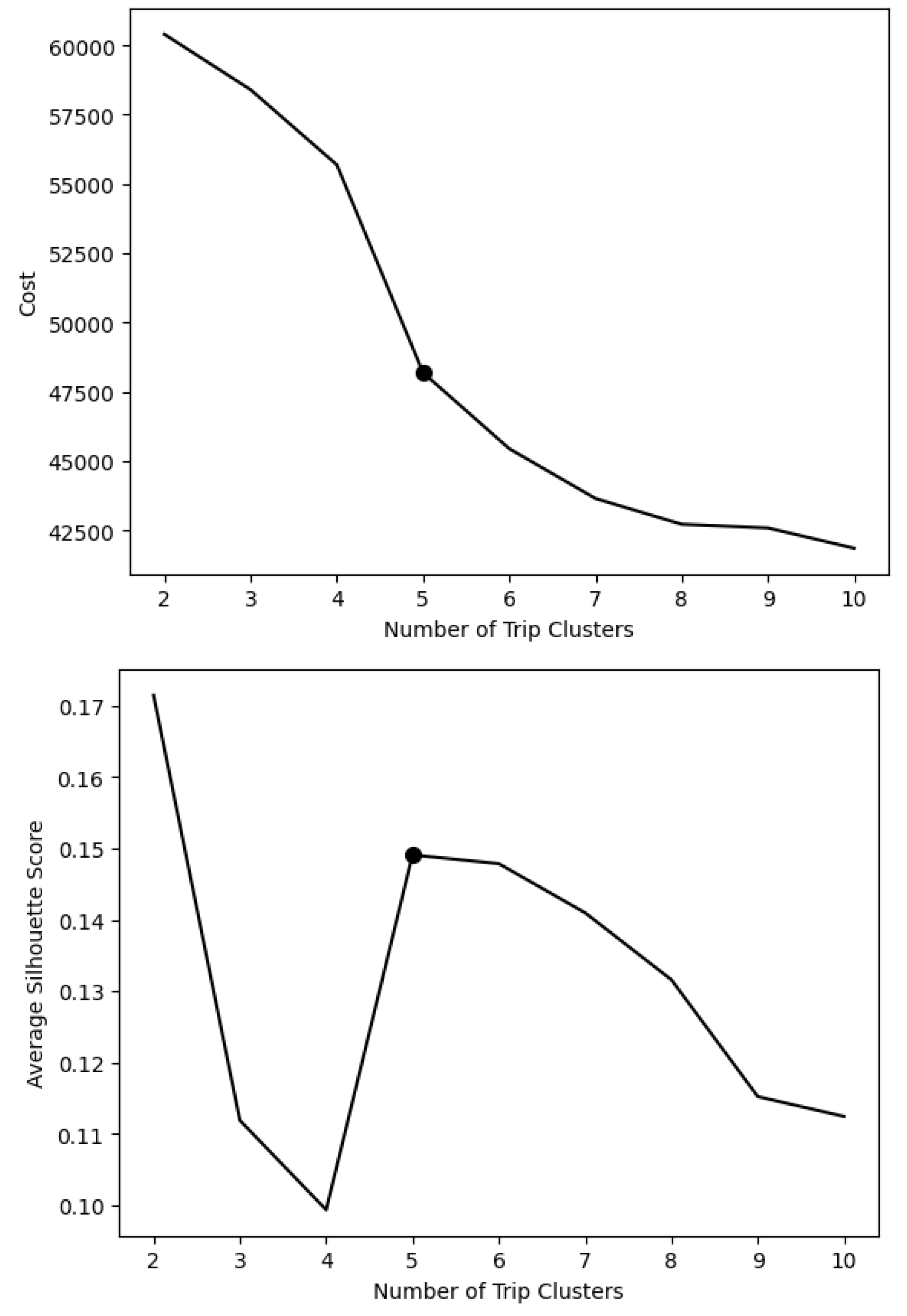
As mentioned earlier, k-modes clustering models with clusters ranging from 2 to 10 were tested and compared based on the elbow plot, silhouette score (Rousseeuw, 1987) and cluster separation. Figure 3 shows the elbow plot and the silhouette scores. An “elbow” (the point with the most significant reduction in cost) in the elbow plot and a higher value for the silhouette score indicates the optimal number of clusters. The silhouette score indicates that there are two candidate models: the 2-cluster model and the 5-cluster model. Even though the 2-cluster model rank higher based on the silhouette score, its cost is also higher in the elbow plot. And it was found that there wasn’t a clear separation between the 2 clusters based on the trip attributes used for clustering. Hence, based on the elbow plot and upon closer inspection of the cluster separation, the 5-cluster model was selected as the final model.

Figure 3. Comparison of k-modes clustering models based on the elbow plot (left) and Silhouette score (right).

Figure 3. Comparison of k-modes clustering models based on the elbow plot (left) and Silhouette score (right).

5.1.2. Model Interpretation

Table 3 shows the names of the 5 trip clusters resulting from the final model and the proportions of different trip attributes for the clusters. Every trip cluster had a dominant characteristic (represented by bold typeface in ) for each trip attributes.

Table 3. Proportion of different trip attributes for the 5 trip clusters.

Trip Attribute		Trip Clusters
		Cluster 1	Cluster 2	Cluster 3	Cluster 4	Cluster 5
		(8060 trips)	(4956 trips)	(2075 trips)	(2249 trips)	(2485 trips)
Weekday/Weekend	Weekday trip	86%	90%	88%	74%	20%
	Weekend trip	14%	10%	12%	26%	80%
Starting time	10 AM - 3 PM	60%	11%	17%	19%	56%
	12 AM - 6 AM	1%	7%	2%	1%	1%
	3 PM - 7 PM	18%	6%	64%	60%	17%
	6 AM - 10 AM	15%	75%	14%	13%	17%
	7 PM - 12 AM	6%	2%	3%	6%	8%
Home-based/non-home based	Home-based trip	22%	81%	76%	25%	75%
	non-home-based trip	78%	19%	24%	75%	25%
Trip Purpose	Errands	19%	6%	47%	10%	6%
	Others	7%	13%	13%	11%	12%
	Shopping or Dining	58%	6%	23%	24%	64%
	Social or recreational	6%	12%	15%	51%	16%
	Work	9%	63%	2%	4%	2%
Dwelling time (time spent at destination)	1-15 minutes	51%	9%	32%	10%	16%
	15-50 minutes	29%	8%	49%	16%	25%
	50-150 minutes	14%	18%	16%	60%	52%
	More than 150 minutes	5%	66%	4%	14%	8%
Trip Distance	0-2 miles	33%	29%	13%	27%	21%
	2-5 miles	43%	17%	19%	19%	19%
	5-15 miles	15%	28%	62%	16%	49%
	More than 15 miles	9%	26%	6%	38%	11%
Number of Passengers	1 passenger	67%	82%	63%	11%	11%
	2-4 passengers	32%	17%	35%	86%	86%
	5 - 10 passengers	2%	1%	1%	3%	3%

Note: The bold typeface indicates the dominant characteristic of the corresponding cluster.

Table 3. Proportion of different trip attributes for the 5 trip clusters.

Trip Attribute		Trip Clusters
		Cluster 1	Cluster 2	Cluster 3	Cluster 4	Cluster 5
		(8060 trips)	(4956 trips)	(2075 trips)	(2249 trips)	(2485 trips)
Weekday/Weekend	Weekday trip	86%	90%	88%	74%	20%
	Weekend trip	14%	10%	12%	26%	80%
Starting time	10 AM - 3 PM	60%	11%	17%	19%	56%
	12 AM - 6 AM	1%	7%	2%	1%	1%
	3 PM - 7 PM	18%	6%	64%	60%	17%
	6 AM - 10 AM	15%	75%	14%	13%	17%
	7 PM - 12 AM	6%	2%	3%	6%	8%
Home-based/non-home based	Home-based trip	22%	81%	76%	25%	75%
	non-home-based trip	78%	19%	24%	75%	25%
Trip Purpose	Errands	19%	6%	47%	10%	6%
	Others	7%	13%	13%	11%	12%
	Shopping or Dining	58%	6%	23%	24%	64%
	Social or recreational	6%	12%	15%	51%	16%
	Work	9%	63%	2%	4%	2%
Dwelling time (time spent at destination)	1-15 minutes	51%	9%	32%	10%	16%
	15-50 minutes	29%	8%	49%	16%	25%
	50-150 minutes	14%	18%	16%	60%	52%
	More than 150 minutes	5%	66%	4%	14%	8%
Trip Distance	0-2 miles	33%	29%	13%	27%	21%
	2-5 miles	43%	17%	19%	19%	19%
	5-15 miles	15%	28%	62%	16%	49%
	More than 15 miles	9%	26%	6%	38%	11%
Number of Passengers	1 passenger	67%	82%	63%	11%	11%
	2-4 passengers	32%	17%	35%	86%	86%
	5 - 10 passengers	2%	1%	1%	3%	3%

Note: The bold typeface indicates the dominant characteristic of the corresponding cluster.

For instance, in trip cluster 1, 58% of trips are made for shopping or dining purposes, occurring mainly on weekdays (86%). These trips typically involve spending little time at the destination (1-15 minutes for 51% of the trips) and cover short distances (43% between 2-5 miles).

Trip cluster 2 is primarily made up of work trips (63%), typically starting between 6 AM and 10 AM (75%). As expected from work trips, these trips often involve longer durations at the destination (over 150 minutes in 66% of cases).

Trip cluster 3 contains trips that are mostly made to run some errands 47% of the time. They are usually home-based trips (76%) that take place during the weekdays (88%).

Trip cluster 4 is predominantly made up of social or recreational trips (51%). As expected for most social and recreational trips, these trips usually have 2-4 passengers (86%) and involve spending 50-150 minutes at the destination in 60% of the cases. The majority of the trips in this cluster are greater than 15 miles (38%).

Trip cluster 5, similar to Cluster 1, also has shopping or dining as the dominant trip purpose. However, there are some key distinctions. Unlike cluster 1, the trips in luster 5 mostly have 2-4 passengers (86%) and they are primarily made during the weekends (80%). Since people have more time to spare during the weekends, these trips involve spending a longer time (50-150 minutes dwelling time) at the destination in 52% of the cases. On the other hand, majority (51%) of the trips in cluster 1 involve spending 1-15 minutes at the destination. These distinctions (between trips in clusters 1 and 5) have been captured by the clustering model (as highlighted in Table 3), which underscores the importance of capturing trip heterogeneity with a two-step modeling framework.

5.2. Classification Model

5.2.1. Model Comparison

As previously mentioned, the classification models were evaluated based on cross-validation accuracy, and testing accuracy. Table 4 presents the results of these metrics. Among the models, the decision tree demonstrated superior performance. While the accuracies of the three machine learning models were quite similar, there was a notable decrease in accuracy for the binary logit model. This discrepancy in accuracy further supports the preference for a machine learning model over traditional discrete choice models in the context of this study. Additionally, the significant difference in accuracy suggests the presence of non-linear relationships that the binary logit model failed to capture. For this specific study, ensemble techniques (random forest and XG boost) did not improve the prediction accuracy of a decision tree for unseen data, as suggested by the cross-validation and testing accuracies. However, if more complex relationships were modeled or a higher dimensional dataset was used, then the ensemble techniques would likely outperform the decision tree. In the following section, the best-performing machine learning model (the decision tree) will be examined in terms of its interpretation. This analysis aims to confirm the existence of non-linear relationships and provide insights into their nature.

Table 4. Comparison of accuracies of the classification models.

Model	Cross-validation Accuracy	Training Accuracy	Testing Accuracy
Decision Tree	88%	98.9%	87.3%
Random Forest	84.5%	98.9%	82.6%
XG Boost	87.1%	97.2%	86.2%
Binary Logit	57.7%	57.6%	57.8%

Table 4. Comparison of accuracies of the classification models.

Model	Cross-validation Accuracy	Training Accuracy	Testing Accuracy
Decision Tree	88%	98.9%	87.3%
Random Forest	84.5%	98.9%	82.6%
XG Boost	87.1%	97.2%	86.2%
Binary Logit	57.7%	57.6%	57.8%

5.2.2. Model Interpretation

5.2.2.1. Variable Importance

The variable importance generally represents the change in the performance of the model in response to the change in the value of an input variable. The metric represents the predictive power of a variable in the model. The importance of the variables used in the decision tree is shown in Figure 4. Upon initial inspection, it can be noticed that the continuous variables (trip day gas price, driver’s age, employment density and population density) contribute more to the predictive power of the model as compared to the discrete variables. The trip day gas price (0.331) is the most important continuous predictor in the model. Among the discrete variables, the trip clusters (0.073) was found to be the most important, which underscores the importance of clustering the trips in the modeling framework.

Figure 4. The variables in the decision tree model arranged in ascending order of variable importance.

Figure 4. The variables in the decision tree model arranged in ascending order of variable importance.

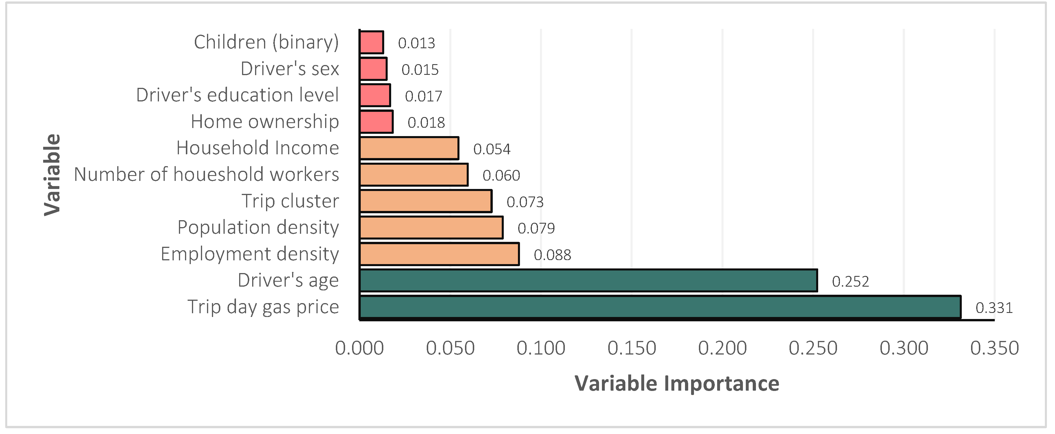
Among the driver attributes, the age (0.252) of the driver was significantly more important than the sex (0.015) and education level (0.017) of the driver in predicting the vehicle choice of a driver in a multi-vehicle household. Among the household attributes, the number of household workers (0.054) was found to be the most important. While variable importance offers insights into the contribution of each variable to the model's accuracy, it is important to note that it does not provide information about the magnitude and direction of their effects on vehicle choice.

5.2.2.2. Accumulated Local Effects

Accumulated local effects (ALE) allow for the estimation of the marginal effects of variables on vehicle choice. ALE is the main effect of a variable at a specific value, relative to the average prediction value of the data. Through this method, complex non-linear relationships between variables can be captured. Figure 5 and Figure 6 shows the ALE plots of each of the variables in the model. The plots show the marginal effects on the choice probability of EV for different values of the variables.

Figure 5. The accumulated local effect (ALE) plots of the trip cluster and household attributes for the decision tree model. The black dots (joined by the broken lines or continuous lines) indicate the effect of the variables at a specific value. The light blue bars indicate number of observations for a specific value of a variable.

Figure 5. The accumulated local effect (ALE) plots of the trip cluster and household attributes for the decision tree model. The black dots (joined by the broken lines or continuous lines) indicate the effect of the variables at a specific value. The light blue bars indicate number of observations for a specific value of a variable.

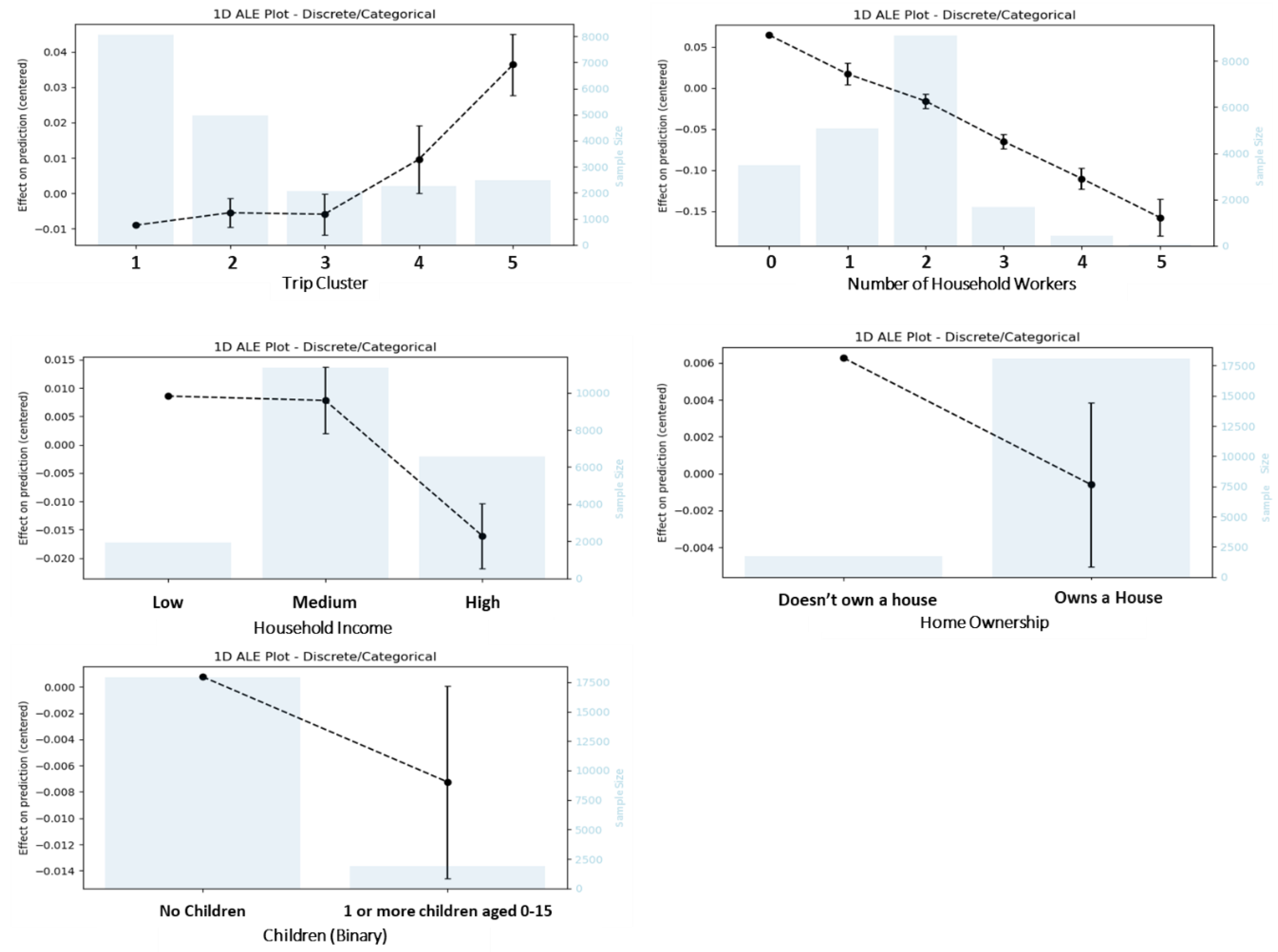
From the ALE plot of trip clusters, we can see that the first three trip clusters have a negative effect on EV choice probability, implying that multi-vehicle households prefer their CVs for making a trip from these trip clusters. On the other hand, trip Clusters 4 and 5 have positive effects (ALE of 0.009 and 0.037 respectively) on the choice probability of EV. This trip-making behavior has some important implications. Firstly, it implies that multi-vehicle households prefer to reserve their EVs for trips that are less frequent, less time-sensitive and discretionary in nature. For instance, both trip clusters 4 and 5 (which have positive effects on EV choice probability) include carpooling (2-4 passengers) trips. These trips are less common in the US compared to the single occupancy trips observed in cluster 1,2, and 3; the average car occupancy in 2017 was 1.5 passengers per vehicle (U.S. Department of Energy (DOE) Oak Ridge National Laboratory, 2022). Additionally, trip cluster 5 (which has the largest positive effect on EV choice probability) primarily serve the discretionary purposes of shopping and dining (Table 3). Although trip cluster 1 also predominantly serve shopping and dining purposes, it has a negative effect on EV choice probability. This may be because trips in cluster 1 are more time-sensitive in nature (mostly involve spending 1-15 minutes at the destination compared to 50-150 minutes for trip cluster 5). Moreover, trip cluster 5 (which has the largest positive effect on EV choice probability) are made during the weekends 80% of the time (Table 3). This finding aligns well with a Swedish study on two-car households (Karlsson, 2020), which found that the driving distance of EVs is 80% greater than CVs during the weekends. The discretionary nature of EV trips can be partly explained by the disparity between the charging time for EVs and CVs (at least 30 minutes for HEVs compared to 5 minutes for a CV) (K. V. Singh et al., 2019). Moreover, EVs are usually associated with higher insurance payments (Parker et al., 2021) and greater sensitivity to external environments. Given the disparity in charging time, sensitivity and higher insurance payments, multi-vehicle households might prefer to reserve their EVs for trips that are less frequent, less time-sensitive and discretionary in nature. Secondly, the trip-making behavior also has some implications on recharging/refueling station locations. If government agencies and other stakeholders want to keep station locations consistent with trip-making behavior, then there should be active efforts to place more charging stations near discretionary trip attractors (e.g., shopping malls, restaurants). On the other hand, if government agencies intends to change people’s behavior and encourage more frequent trips from EVs, placing stations near frequent trips attractors could be a possible course of action.

As the number of household workers goes up, the choice probability of EV goes down steadily (Figure 5). This may be attributed to the higher number of ICEVs (compared to EVs) in households with higher number of workers. For instance, an analysis of the dataset used in this study shows that the average number of ICEVs in households with 3 or more workers is 3. In the same households, the average number of EVs is 1.

From the ALE plot of household income (Figure 5), it is evident that households falling under the low income (ALE = 0.0057) and medium-income categories (ALE = 0.0058) are more likely to choose their EV for a trip than households in the high-income category (ALE = 0.0155). The lower-income households might be inclined to use EVs more because of their fuel efficiency. Previous studies have shown that EVs can be expected to achieve cost-effectiveness in multi-vehicle households within six years (Jakobsson et al., 2016a) as they make up for their high purchase price through their fuel efficiency. Given the effects of income and number of household workers, the policy makers should have dedicated EV incentives for households with lower income and lower number of workers. Currently, households with a higher income are more likely to own EVs (Liu et al., 2019). If incentives reduce the purchase price of EVs for lower-income households, we can expect more EV usage.

The ALE plot of children indicates that households with one or more children prefer ICEVs and households with no children prefer EVs (Figure 5). This could be true because households with children are likely to have more members, thereby need higher occupancy vehicles (e.g., minivans). Most of these higher occupancy vehicles in the NHTS 2017 dataset are ICEVs, which explains their preference for ICEVs over EVs. Hence households with one or more children may represent a segment of the market that EV manufacturers can further tap into by producing higher occupancy light-duty vehicles.

Figure 6. The accumulated local effect (ALE) plots of driver attributes, gas price and built environment variables for the decision tree model. The black dots (joined by the broken lines or continuous lines) indicate the effect of the variables at a specific value. The light blue bars indicate number of observations for a specific value of a variable.

Figure 6. The accumulated local effect (ALE) plots of driver attributes, gas price and built environment variables for the decision tree model. The black dots (joined by the broken lines or continuous lines) indicate the effect of the variables at a specific value. The light blue bars indicate number of observations for a specific value of a variable.

Observing the ALE plot for driver age (Figure 6) tells us that age has a multi-linear relationship with EV choice. It is clear from the plot that EV choice probability linearly goes up as age goes up until 30. However, the relationship is no longer clear after 30 years. Even though age was the second most important predictor, the marginal effect of age above 30 is not discernible. It is possible that the effect of age on vehicle choice in these households may also vary geographically within the US, similar to the effect of age on adoption (Liu et al., 2019). This might be a reason why the national sample could not capture a clear relationship between EV choice and age beyond 30.

As indicated by the ALE plot of driver’s education level (Figure 6), the probability of a driver choosing the EV is higher when he/she has a bachelor’s degree or higher education (ALE=0.03). This is consistent with the findings from studies on EV adoption which suggest that education level has a positive effect on adoption (Liu et al., 2019). A higher level of education is generally associated with a higher concern for the environment, which might cause people to choose their EVs.

The ALE plots of driver’s sex indicate that the women in multi-vehicle households are more likely to drive EVs compared to men (Figure 6). This finding may be attributable to vehicle access in these households. A previous study on car deficient households (houses with a lower number of cars than drivers) has found that men have more access to the household car than women (Tiikkaja and Liimatainen, 2021). In multi-vehicle households with EVs and ICEVs, the same phenomenon may apply to ICEVs; the female members may have lower access to the ICEVs, which may make them more likely to drive EVs.

Trip day gas price, similar to age, has a multi-linear relationship with EV choice probability (Figure 6). Trip day gas price had the highest predictive power among all the variables. The ALE plot indicates that the gas price does not have a clear effect on EV choice as long as the gas price is below 2.80 USD per gallon. However, when the gas price goes above 2.80 USD per gallon, we start to notice a clear positive effect on EV choice probability. Previous studies have suggested making conventional fuels more expensive as a strategy to promote EV use (Parker et al., 2021). The threshold of $2.80 for gas price can be used to implement such strategies. However, this threshold has to be adjusted for inflation since the data for this study is from 2017. Nevertheless, this valuable information could not have been extracted from a discrete-choice model that assumes a linear relationship.

The ALE plots of the built environment variables (employment density and population density) appear to have opposite effects on vehicle choice (Figure 6). The marginal effects for the built environment variables do not show a steady increase or decrease. In general, the larger values of employment density have positive effects on EV choice probability, while the smaller values have negative effects. Whereas for the larger values of population density, the marginal effects on EV choice probability are negative. Population density was also found to have a negative effect on the VMT of PEVs in multi-vehicle households (Chakraborty et al., 2022). This negative effect might be explained by the higher number of publicly available charging stations in suburban areas compared to urban areas (Brown et al., 2022).

6. Conclusion

This study investigates the factors that influence vehicle choice for trips in multi-vehicle households in the US, specifically those with at least one EV and one ICEV. A two-step machine learning modeling framework was employed, starting with k-modes clustering to identify 5 distinct trip clusters that captured the heterogeneity in trips. Subsequently, a decision tree model was employed to predict vehicle choice (EV or ICEV). A comparison of four different modeling approaches was performed before the decision tree was chosen as the final model in the modeling framework. The comparison of the models revealed that the decision tree (cross-validation accuracy of 88%) outperformed the binary logit (cross-validation accuracy of 57.7%) by a large margin. Notably, trip day gas price and the driver's age were found to be major contributors to decision tree's predictive power. Both of these variables had non-linear effects on EV preference, which the binary logit model would be unable to capture. This further underscores the significance of employing machine learning approaches, such as decision trees, within the context of this study.

ALE plots were produced to analyze the effects of different variables on vehicle choice, as captured by the decision tree model. The analysis revealed that weekend trips primarily intended for shopping and dining were most likely to be made using EVs, indicating the discretionary use of EVs within multi-vehicle households. To keep the locations of charging stations consistent with travel behavior, these stations may be placed near popular shopping and dining destinations. Conversely, these stations may be placed near frequent trip attractors (e.g., locations with high employment density) if the policymakers intend to encourage owners to use EVs for non-discretionary/frequent trips. Other factors such as the number of household workers, income, and trip day gas price also exhibited noticeable effects on vehicle choice. Overall, multi-vehicle households with lower income and fewer workers were more inclined to choose EVs for their daily trips. However, these households face challenges in adopting EVs initially due to the higher purchase prices. To promote higher EV usage, targeted incentives should be implemented to make EVs more affordable for these households. Additionally, gas prices exceeding $2.80 USD per gallon were found to discourage the use of ICEVs within multi-vehicle households, suggesting that gas prices can serve as a tool to increase EV usage.

It is important to acknowledge a few limitations of this study. Due to the limited number of trips made by PHEVs and BEVs, they were considered in a single category along with HEVs. This may potentially overlook differences between these vehicle types. Furthermore, the NHTS 2017 dataset predominantly includes older EV models, which are gradually being replaced by newer models with extended ranges. These limitations of the study should be taken into account by decision makers and the findings of this study should be complemented with those from future studies before taking policy decisions. Such future studies can leverage datasets that encompass trip data from newer EV models, enabling the modeling of vehicle choices for different EV categories separately.

References

- Apley, D.W., Zhu, J., 2020. Visualizing the effects of predictor variables in black box supervised learning models. J R Stat Soc Series B Stat Methodol 82. [CrossRef]
- Bhat, C.R., 1997. Work Travel Mode Choice and Number of Non-Work Commute Stops. Transportation Research Part B: Methodological 31, 41–54ode Choice and Number of Non-Work Commute Stops. Transportation Research Part B: Methodological 31, 41–54. [CrossRef]
- Biau, G., Scornet, E., 2016. A random forest guided tour. Test 25, 197–227. [CrossRef]
- Breiman, L., 2001. Random Forests. Mach Learn 45, 5–32.
- Breiman, L., 1984. Classification and Regression Trees, 1st ed. Chapman and Hall/CRC.
- Brown, A., Cappellucci, J., Schayowitz, A., White, E., Heinrich, A., Cost, E., 2022. Electric Vehicle Charging Infrastructure Trends from the Alternative Fueling Station Locator: First Quarter 2022.
- Bucher, D., Martin, H., Hamper, J., Jaleh, A., Becker, H., Zhao, P., Raubal, M., 2020. Exploring Factors that Influence Individuals’ Choice Between Internal Combustion Engine Cars and Electric Vehicles. AGILE: GIScience Series 1, 1–23. [CrossRef]
- Cameron, A.C., Trivedi, P.K., 2010. Microeconometrics using stata. Stata press, College Station, TX.
- Cao, F., Liang, J., Bai, L., 2009. A new initialization method for categorical data clustering. Expert Syst Appl 36, 10223–10228. [CrossRef]
- Carlucci, F., Cirà, A., Lanza, G., 2018. Hybrid electric vehicles: Some theoretical considerations on consumption behaviour. Sustainability 10. [CrossRef]
- Caulfield, B., Farrell, S., McMahon, B., 2010. Examining individuals preferences for hybrid electric and alternatively fuelled vehicles. Transp Policy (Oxf) 17, 381–387. [CrossRef]
- Chakraborty, D., Hardman, S., Tal, G., 2022. Integrating plug-in electric vehicles (PEVs) into household fleets- factors influencing miles traveled by PEV owners in California. Travel Behav Soc 26, 67–83. [CrossRef]
- Chaturvedi, A., Green, P.E., Caroll, J.D., 2001. K-modes Clustering. J Classif 18, 35–55.
- Chen, T., Guestrin, C., 2016. XGBoost: A scalable tree boosting system, in: Proceedings of the ACM SIGKDD International Conference on Knowledge Discovery and Data Mining. Association for Computing Machinery, pp. 785–794. [CrossRef]
- De Borger, B., Mulalic, I., Rouwendal, J., 2016. Substitution between cars within the household. Transp Res Part A Policy Pract 85, 135–156. [CrossRef]
- Egbue, O., Long, S., 2012. Barriers to widespread adoption of electric vehicles: An analysis of consumer attitudes and perceptions. Energy Policy 48, 717–729. [CrossRef]
- Friedman, J.H., 2001. Greedy Function Approximation: A Gradient Boosting Machine. The Annals of Statistics 29, 1189–1232.
- Ghandi, A., Paltsev, S., 2020. Global CO2 impacts of light-duty electric vehicles. Transp Res D Transp Environ 87. [CrossRef]
- Hackbarth, A., Madlener, R., 2013. Consumer preferences for alternative fuel vehicles: A discrete choice analysis. Transp Res D Transp Environ 25, 5–17. [CrossRef]
- Hardman, S., Chandan, A., Tal, G., Turrentine, T., 2017. The effectiveness of financial purchase incentives for battery electric vehicles – A review of the evidence. Renewable and Sustainable Energy Reviews 80, 1100–1111. [CrossRef]
- Huang, Z., 1998. Extensions to the k-Means Algorithm for Clustering Large Data Sets with Categorical Values. Data Min Knowl Discov 12, 283–304he k-Means Algorithm for Clustering Large Data Sets with Categorical Values. Data Min Knowl Discov 12, 283–304.
- Jakobsson, N., Gnann, T., Plötz, P., Sprei, F., Karlsson, S., 2016a. Are multi-car households better suited for battery electric vehicles? - Driving patterns and economics in Sweden and Germany. Transp Res Part C Emerg Technol 65, 1–15. [CrossRef]
- Jakobsson, N., Karlsson, S., Sprei, F., 2016b. How are driving patterns adjusted to the use of a battery electric vehicle in two-car households?, in: Electric Vehicle Symposium.
- Jakobsson, N., Sprei, F., Karlsson, S., 2022. How do users adapt to a short-range battery electric vehicle in a two-car household? Results from a trial in Sweden. Transp Res Interdiscip Perspect 15. [CrossRef]
- Jensen, A.F., Mabit, S.L., 2015. MODELLING REAL CHOICES BETWEEN CONVENTIONAL AND ELECTRIC CARS FOR HOME-BASED JOURNEYS, in: Annual Transport Conference at Aalborg University.
- Jia, J., 2019. Analysis of Alternative Fuel Vehicle (AFV) Adoption Utilizing Different Machine Learning Methods: A Case Study of 2017 NHTS. IEEE Access 7, 112726–112735. [CrossRef]
- Karlsson, S., 2020. Utilization of battery-electric vehicles in two-car households: Empirical insights from Gothenburg Sweden. Transp Res Part C Emerg Technol 120. [CrossRef]
- Kim, E.J., 2021. Analysis of Travel Mode Choice in Seoul Using an Interpretable Machine Learning Approach. J Adv Transp 2021. [CrossRef]
- Kim, S., Gudmundur F. Ulfarsson, 2004. Travel mode choice of the elderly- effects of personal, household, neighborhood, and trip Characteristics. Transp Res Rec 1894, 117–126. [CrossRef]
- Li, X., Liu, C., Jia, J., 2019. Ownership and usage analysis of alternative fuel vehicles in the United States with the 2017 National Household Travel Survey data. Sustainability 11. [CrossRef]
- Liaw, A., Wiener, M., 2002. Classification and Regression by randomForest.
- Liu, J., Khattak, A.J., Li, X., Fu, X., 2019. A spatial analysis of the ownership of alternative fuel and hybrid vehicles. Transp Res D Transp Environ 77, 106–119. [CrossRef]
- Mandev, A., Sprei, F., Tal, G., 2022. Electrification of Vehicle Miles Traveled and Fuel Consumption within the Household Context: A Case Study from California, U.S.A. World Electric Vehicle Journal 13. [CrossRef]
- Musti, S., Kockelman, K.M., 2011. Evolution of the household vehicle fleet: Anticipating fleet composition, PHEV adoption and GHG emissions in Austin, Texas. Transp Res Part A Policy Pract 45, 707–720. [CrossRef]
- Myles, A.J., Feudale, R.N., Liu, Y., Woody, N.A., Brown, S.D., 2004. An introduction to decision tree modeling. J Chemom. [CrossRef]
- Ozhegov, E.M., Ozhegova, A., 2019. Heterogeneity in demand and optimal price conditioning for local rail transport. arXiv:1905.12859v1 [econ.EM]. arXiv:1905.12859v1 [econ.EM].
- Pandit, S., Gupta, S., 2011. A comparative study on distance measuring approaches for clustering. International Journal of Research in Computer Science 2, 29–31. [CrossRef]
- Parker, N., Breetz, H.L., Salon, D., Conway, M.W., Williams, J., Patterson, M., 2021. Who saves money buying electric vehicles? Heterogeneity in total cost of ownership. Transp Res D Transp Environ 96D Transp Environ 96. [CrossRef]
- Perez, J., 2020. The Fastest Cars You Can Buy From Every Automaker [WWW Document]. URL https://www.motor1.com/features/428317/fastest-cars-from-every-automaker/.
- Rousseeuw, P.J., 1987a. Silhouettes: a graphical aid to the interpretation and validation of cluster analysis, Journal of Computational and Applied Mathematics.
- Rousseeuw, P.J., 1987b. Silhouettes: a graphical aid to the interpretation and validation of cluster analysis. J Comput Appl Math 20, 53–65.
- en, Chitradeep., 2010. Performance analysis of batteries used in electric and hybrid electric vehicles. University of Windsor, Windsor, Ontario, Canada.
- Sherman, L., 1980. Implications of current household vehicle ownership and use patterns on the feasibility of electric cars. Transportation (Amst) 9, 209–227. [CrossRef]
- Shin, H.-S., Farkas, Z.A., Nickkar, A., 2019. An Analysis of Attributes of Electric Vehicle Owners’ Travel and Purchasing Behavior: The Case of Maryland, in: International Conference on Transportation and Development 2019: Innovation and Sustainability in Smart Mobility and Smart Cities. American Society of Civil Engineers, Reston, VA, pp. 77–90.
- Singh, Virender, Singh, Vedant, Vaibhav, S., 2020. A review and simple meta-analysis of factors influencing adoption of electric vehicles. Transp Res D Transp Environ 86. [CrossRef]
- Soltani-Sobh, A., Heaslip, K., Stevanovic, A., Bosworth, R., Radivojevic, D., 2017. Analysis of the Electric Vehicles Adoption over the United States. Transportation Research Procedia 22, 203–212212. [CrossRef]
- Srinivasa Raghavan, S., Tal, G., 2021. Behavioral and technology implications of electromobility on household travel emissions. Transp Res D Transp Environ 94. [CrossRef]
- Tamor, M.A., Milačić, M., 2015. Electric vehicles in multi-vehicle households. Transp Res Part C Emerg Technol 56, 52–60. [CrossRef]
- Tanaka, M., Ida, T., Murakami, K., Friedman, L., 2014. Consumers’ willingness to pay for alternative fuel vehicles: A comparative discrete choice analysis between the US and Japan. Transp Res Part A Policy Pract 70, 194–209. [CrossRef]
- Tiikkaja, H., Liimatainen, H., 2021. Car access and travel behaviour among men and women in car deficient households with children. Transp Res Interdiscip Perspect 10. [CrossRef]
- Tompkins, M., Bunch, D., Santini, D., Bradley, M., Vyas, A., Poyer, D., 1998. Determinants of alternative fuel vehicle in the continental united states choice. Transp Res Rec 1641, 130–138. [CrossRef]
- U.S. Department of Energy, 2013. Alternative Fuels Data Center.
- U.S. Department of Transportation, 2017. 2017 National Household Travel Survey.
- ergis, S., Chen, B., 2014. Understanding variations in U.S. plug-in electric vehicle markets, Transportation Research Board 94th Annual Meeting. Transportation Research Board, Davis, CA.
- Wang, F., Ross, C.L., 2018. Machine Learning Travel Mode Choices: Comparing the Performance of an Extreme Gradient Boosting Model with a Multinomial Logit Model. Transp Res Rec 2672, 35–45. [CrossRef]
- Yang, Y., Wang, C., Liu, W., Zhou, P., 2018. Understanding the determinants of travel mode choice of residents and its carbon mitigation potential. Energy Policy 115, 486–493. [CrossRef]
- Zhao, X., Yan, X., Yu, A., Van Hentenryck, P., 2020. Prediction and behavioral analysis of travel mode choice: A comparison of machine learning and logit models. Travel Behav Soc 20, 22–35. [CrossRef]
- Zulinski, J., 2018. U.S. Leads in Greenhouse Gas Reductions, but Some States Are Falling Behind [WWW Document]. URL https://www.eesi.org/articles/view/u.s.-leads-in-greenhouse-gas-reductions-but-some-states-are-falling-behind.
Disclaimer/Publisher’s Note: The statements, opinions and data contained in all publications are solely those of the individual author(s) and contributor(s) and not of MDPI and/or the editor(s). MDPI and/or the editor(s) disclaim responsibility for any injury to people or property resulting from any ideas, methods, instructions or products referred to in the content. |
© 2024 by the authors. Licensee MDPI, Basel, Switzerland. This article is an open access article distributed under the terms and conditions of the Creative Commons Attribution (CC BY) license (http://creativecommons.org/licenses/by/4.0/).
Copyright: This open access article is published under a Creative Commons CC BY 4.0 license, which permit the free download, distribution, and reuse, provided that the author and preprint are cited in any reuse.