
Submitted:
10 May 2024
Posted:
12 May 2024
You are already at the latest version
Abstract
An Oscillating Water Column device, specifically a Savonius turbine, underwent comprehensive testing within an air duct to evaluate its performance under varying rotational speeds, flow directions, and the presence of power augmenters positioned both in front of and behind the device. The experimental setup involved the utilization of load cells and pressure transducers, with their data utilized to calculate pressure differentials across the turbine and torque. Subsequently, a predictive model based on decision trees was developed using Machine Learning. This model was then used to analyze the influence of various features on predicting the pressure difference, considered as the output. The results of the validation (10-fold cross-validation) and test phases were thoroughly investigated. Moreover, obtaining a predictive model allows for the exploration of different scenarios without relying solely on physical experimentation, thereby broadening the scope for further testing.
Keywords:
OWC
; Machine Learning
; Savonius
; Predictive Model
1. Introduction
The energy and environmental challenges stand as major issues that humanity faces in the 21st century [1]. The escalating demand for energy, propelled by population growth and economic development, has led to a surge in greenhouse gas emissions, climate change, environmental degradation, and the depletion of natural resources.
At the forefront of global challenges lie climate change, resource scarcity—particularly in terms of energy—and environmental pollution. The former is inextricably linked to the surge in greenhouse gas emissions, predominantly driven by the widespread utilization of fossil fuels [2,3,4,5,6], resulting in climate shifts such as rising sea levels, intensified weather events, and ecosystem disruptions.
Moreover, the energy demand, currently heavily reliant on oil, coal, and natural gas, has precipitated a gradual depletion of resources. Simultaneously, the use of fossil fuels has engendered significant pollution, detrimentally impacting the environment and human health.
Addressing the environmental repercussions of energy consumption necessitates a fundamental shift in the energy landscape towards renewable energy sources, efficient energy carriers [7,8,9,10,11,12] and different manufacturing processes [13,14].
Optimizing energy use through enhanced energy efficiency in end-use applications plays a crucial role in mitigating adverse climate impacts. Another compelling strategy to reduce dependency on traditional energy sources and mitigate environmental harm is tapping into ocean energy, notably wave energy. Despite its initial high installation costs and relatively lower efficiency, wave energy extraction presents a promising avenue for energy supply.
Among various wave energy conversion technologies, Oscillating Water Column (OWC) systems have emerged as particularly promising options [15,16]. These systems comprise a partially submerged chamber with an underwater opening on its front side and an air turbine. When waves interact with the device, the water column within the chamber undergoes oscillations, thus earning the system its name. These oscillations act akin to a piston, causing airflow alternation between exiting and entering the chamber's upper section. This cyclic airflow propels the turbine, thereby generating power.
The Savonius turbine can serve as an effective power take-off mechanism in OWC systems for efficient wave energy harnessing at a low cost [17,18].
In this study, experimental tests were made, and the data was processed using machine learning algorithms to assess the factors influencing turbine performance. The utilization of Machine Learning (ML) techniques allowed for a comprehensive evaluation of various parameters affecting turbine efficiency. The outcome of this evaluation can be used to set an optimization process to enhance performance or efficiency as it’s already being done in different engineering fields [19,20,21].
The performance of the turbine can be influenced by deflectors positioned upwind or downwind of the turbine [22,23,24].
In this research, the Bell-Metha polynomial law was used to design power augmenters that act as convergent ducts. These augmenters can be strategically placed both upwind and downwind of the turbine to enhance its performance. By employing this approach, the rotational speed of the turbine increases, thereby influencing its overall efficiency. A Machine Learning (ML) algorithm based on decision trees was subsequently implemented to extract insights into the parameters exerting the most significant influence on turbine power production. Furthermore, the utilization of a ML regression model enables the exploration of diverse configurations of the used parameters without necessitating alterations to the setup. The advantage in applying this ML algorithm is the ability to predict the value of the pressure drop (between the upwind and downwind size of the turbine) generated by through new configurations without the use of sensors and to vary the configuration of the real system. The ML approach allows to get the digital part of
Therefore, what can be defined as a partial digital twin of the system is obtained, with which it is possible to test different combinations of parameters to achieve the best performance.
2. Materials and Methods
2.1. Experimental Setup
The experimental tests were conducted in a test tube at the University of Messina (Figure 1). The upper portion of the test tube is constructed with plexiglass walls, forming an internal square cross-section measuring 100×100 mm and extending 1000 mm in length. The turbine is positioned at the midpoint of the upper section.
The lateral regions comprise two curved sections, also with square cross-sections. In the lower section, there are a fan that generates the airflow and a diverter. The diverter can rotate at a preset frequency f, enabling the redirection of airflow towards one of the two curves. When f=0 the flow is mono-directional; when f>0 the flow is bi-directional and the inversion velocity can be controlled.
The layout of the test tube is presented in Figure 2.
The turbine was 3D printed in PLA. The principal characteristics are listed in Table 1.
The airflow is generated by a centrifugal fan, the EBM Papst G1G133-DE19-15, powered by a 24-volt DC voltage. This fan operates at a rotational speed of 2000 r/min and has an outlet section measuring 59x71 mm. In the present study, both mono-directional and bi-directional tests have been conducted. For this purpose, the diverter swings around its hinge, directing the airflow from the fan towards one of the lateral sections depending on its position. The diverter is actuated by a stepper motor and is presented in Figure 3. The bi-directional flow simulates the rising and falling of waves in the sea.
2.1.1. Power Augmenters
The power augmenters have been designed according to the Bell-Metha polynomial.
is the height of the ramp, a generic length expressed in millimeters, the total length of the ramp and the dependent variable defined as x/L (Figure 4).
Depending on the frequency of the diverter, the turbine can be tested both in mono and bi-directional flow conditions.
Different distances between the turbine and the power augmenters have been tried. In mono-directional test cases, only the upwind power augmenter has been placed since the flow has only one clear direction; in the bi-directional tests the power augmenters have been placed both upwind and downwind. In Figure 5, the positioning of the power augmenter with a distance of D/8 in a mono-directional test has been represented.
2.1.2. Measurement Devices
The measurements are made through two velocity sensors, a load cell and two pressure sensors. The analogic board used to process signals from the sensors is the NI cDAQ 9171. These signals are processed and managed using the software LabView on the computer.
The diverter is rotated using a stepper motor and it is operated via an Arduino code, which allows setting the desired rotation frequency.
The connections between all the devices are represented in Figure 6.
Torque Measurement
To measure the torque developed by the turbine, a belt brake composed of a pulley, a nylon wire, a suspended mass and a load cell was employed (Figure 7).
The nylon wire is connected at one end to the load cell fixed to the ground, runs along the pulley, and at the other end, there is a hook with which it is possible to suspend a mass. Since the pulley is keyed to the turbine shaft, its rotation speed varies depending on the suspended mass. Figure 7 shows a schematic of the system used and the balance of dynamic forces.
- : weight force.
- : friction force acting on the pulley.
- : force measured by the load cell.
Under static conditions, since :
However, under dynamic conditions, the force measured by the cell will be:
Pitot Tubes
To calculate the fluid velocity inside the test tube, two Pitot tubes were placed, each at 100 mm from the two bends of the upper section. These are two tubes immersed in the fluid, one facing upstream and the other downstream. Both are equipped with a hole at the front that serves as a total pressure (or stagnation pressure) port. Additionally, longitudinally, at a certain distance, there are additional holes acting as static pressure ports.
The relationship between pressure and velocity is expressed by Bernoulli equation.
The data collected from the Pitot tubes and the pressure taps upstream and downstream of the rotor (ΔP) were processed by a pressure transmitter. Three DeltaOhm HD420T devices were used: two for the Pitot tubes and one to determine the pressure drop near the turbine.
Rotary Encoder
To measure the turbine rotational speed, a rotary encoder was used. Positioned in front of a ring with alternating black and white bands, this device produces a voltage corresponding to the band aligned with the sensor. The resulting signal is a square wave.
Each time the encoder detects a white band, it generates a peak in the signal. The pulses per second (PPS) can be calculated using Eq. 5.
are the total pulses recorded during the test and the recording period in seconds.
Knowing that there are 8 white bands in the encoder, once the pulses per second are calculated, the rotational speed in r/min of the turbine can be calculated.
Data Acquisition
Data collection is divided into two phases: one with the fan turned on and one with the fan turned off. By comparing the data from these two phases, it's possible to evaluate the turbine's torque and effective power since in the second phase, the friction force on the pulley, is zero.
The software used to record the tests is LabView. A recording duration of 20 seconds was set with a sampling frequency of 0.001 s. The force detected by the load cell, the pressure drop measured by the Pitot tubes and the encoder signal in volts were acquired.
Furthermore, to ensure accurate analysis, it was necessary to reset the load cell so that it did not consider the mass of the screw, nylon wire, and hook connected to it, thus evaluating the torque without taking external elements into account.
Since each acquisition has 20,000 data points, it's necessary to calculate the mean of all values obtained to determine the mean value of the airflow velocity , the mean value of between upstream and downstream of the turbine, and the mean value of the applied load .
In particular, the airflow velocity and the applied load can be obtained using Eq. 7-8.
With:
: number of registered data;
load measured with the fan on;
load measured with the fan offThe torque T, the power W of the turbine, and the available power Pin are expressed in Nm and Watt, respectively.
Once these parameters are obtained, the value of the power coefficient and the tip speed ratio are determined.
2.1.3. Tested Configurations
Different configurations have been tested, varying the number and the positioning the Power Augmenters (PA). A complete summary of the conducted tests is presented in Table 2.
The test on a certain configuration is repeated at least five times, to check and ensure the repeatability of the measurement.
2.2. Machine Learning
Machine Learning (ML)[25,26] is a branch of artificial intelligence (AI). It originated in the 1950s in Hanover [27] and focuses on systems that perform tasks that, to an external observer, would appear to be exclusively within the domain of human intelligence. ML emerged as a subset of AI following various schools of thought that defined an "intelligent" system as one capable of learning from experience and improving its performance [28]. This distinctive trait sets ML algorithms apart from conventional computer programming, as they can operate even under conditions for which they haven't been explicitly programmed.
The main objective of testing the physical model with different configurations (frequency, load, number of power augmenters, and power augmenter distance) is to maximize the power output of the turbine. With the same input power (fan), the aim is to maximize the output power (generated by the turbine). As mentioned earlier, one of the fluid parameters measured by dedicated sensors during the various tests is the pressure difference (ΔP) created between the upstream and downstream stages of the turbine. The investigation aimed to identify which parameters, when varied within the different system configurations, had the greatest impact on the generation of ΔP. Understanding which parameters most significantly influence the value of ΔP would allow for coherent modification of the setup to maximize the turbine power output. To recap, the parameters varied during the different tests are applied load, presence/absence of power augmenters, number of power augmenters, flow feed frequency, and distance between the power augmenters. Among these parameters, the presence/absence of power augmenters and the number of power augmenters are categorical variables, unlike all the others which are continuous variables. Table 3. summarizes the setup variables along with a description and range of variation.
The ΔP is evidently a continuous quantity with a variability range of [-151.9606, 85.0614] Pa. This range of ΔP is determined by computing the pressure difference between measurements taken downstream and upstream of the turbine. Thus, the negative sign denotes instances where the downstream pressure surpasses that measured upstream of the turbine (with consideration for potential variations in fluid flow direction). However, for power generation considerations, the absolute value of ΔP is paramount, given the self-aligning property of the Savonius turbine, which rotates unidirectionally regardless of fluid flow direction. Therefore, ΔP is evaluated in absolute terms, as power production remains unaffected by fluid flow direction.
With the available dataset, derived from the measurements taken, it was decided to train a Machine Learning (ML) algorithm for two main reasons:
- To identify the parameters that most influence ΔP.
- To obtain a model capable of hypothesizing new scenarios without the constraint of necessarily intervening on the physical system.
As is well known, an ML algorithm is capable of learning a relationship between the features and the output, even under conditions it has never encountered before, unlike in traditional programming.
The dataset consists of 5 input variables (referred to as "features") and one output variable (ΔP), comprising 1044 instances, or observations. This dataset was then split to obtain three distinct datasets, each for one of the three phases required to develop a robust ML model: training, validation, and testing. Approximately 10% of the dataset (100 instances selected randomly) was reserved for the testing phase, while the remaining data underwent a 10-fold cross-validation. Table 4. provides an overview of the datasets and the number of instances they contain.
This practice is employed to enhance the model's performance, especially when the dataset is not extensive. Consequently, the remaining 90% of the dataset is divided into 9 sections. Ten training and validation sessions are conducted, using 9 sections for training and 1 section for validation during each session.
In each phase, a different section will be used for validation. During validation, the model's performance is evaluated and improved. The unique aspect of using cross-validation is that it not only estimates the performance of the trained model but also provides a measure of how accurate its predictions are (through evaluation of the standard deviation) and how reproducible they are. Finally, the test dataset simulates a real application of the model, aiming to observe its behavior with data it has never seen during training. The test results provide a measure of the model's goodness.
The choice of the ML model to implement fell on decision trees, which are a predictive model based on a tree structure for decision-making. The advantages of this model for the problem addressed in this work will be discussed later.
A decision tree model is a structure composed of nodes and leaves. Each node represents a question or condition about a data attribute, and each leaf represents a class or output value, depending on whether it is a classification or regression problem.
At the beginning of the tree is the root node, which contains the entire training data set. From here, the tree branches into child nodes, each of which represents a possible response to the question or condition posed by the parent node. Each child node is connected to the parent node by a branch, indicating the hierarchical relationship between them. Descending along the tree, encounters with intermediate nodes occur, which continue to pose questions or conditions on the data based on previous answers. This process continues until reaching the tree's leaves, where a final decision is made, or a predictive output is provided. Figure 8. show a schematization of a decision tree.
The algorithm underlying the operation of decision trees is called Classification and Regression Tree (CART). It is used for both classification and regression problems. The problem addressed in this work falls within the realm of regression. Indeed, the output variable is a continuous variable (unlike a classification problem where the output is a class). Therefore, in this case, the model will predict continuous values, and to assess the model's performance, the error in estimating these values is measured.
CART constructs a decision tree by splitting the dataset into two subsets of data according to a feature (k) and a certain threshold (t). The feature is chosen by carefully evaluating the k-t pairs that minimize a certain function. In the case of regression, the goal is not to determine a class but to obtain a value. The cost function to be minimized is based on the Mean Square Error (MSE) and is as follows [29]:
Where:
- MSE is calculated as the average of the squares of the differences between the values predicted by the tree () and the corresponding actual values in the training data (). Minimizing the MSE during tree construction helps find optimal splits that reduce the overall prediction error.
- is the total number of instances in the training dataset.
- represents the number of instances contained in the node of interest.
- The number of instances to the right () and left () refers to the number of training samples ending up in the right and left subtree respectively during the tree splitting process.
This aspect is crucial because during the tree construction phase, the goal is to find splits that minimize predictive error while simultaneously avoiding overfitting. Therefore, the splits must be chosen to minimize the MSE and ensure that each subtree has a sufficient number of instances to make accurate predictions.
Overfitting occurs when a model excessively fits the training data, capturing the noise present in the data rather than just the relevant patterns. In this way, the decision tree runs the risk of becoming too complex, with many splits and nodes, to the point of effectively memorizing the training data instead of being able to generalize correctly to new, unseen data. As a result, the model may fail to generalize, meaning it cannot properly evaluate new data, as it has overfit to the training data.
The choice of a decision tree-based ML algorithm to address the problem proposed in this work is supported by a series of motivations outlined below.
This ML model is capable of working with mixed variables (continuous and categorical) without needing to convert categorical ones into binaries through a process called one-hot encoding. Moreover, they can achieve good performance even with relatively small datasets (on the order of thousands of data points as in the case of the dataset used in this work). The computational burden required for training a decision tree model is very low since they are quickly implementable and do not require data normalization. The most important characteristic of decision trees, for the purposes of this work, is that they behave like white boxes. Unlike many other ML methods such as neural networks, which behave like black boxes, a decision tree model is highly interpretable. Therefore, it is possible to understand how the model makes its prediction. This allows for the identification of the most influential input variables on the output.
To analyze the model's performance, that is, to obtain a quantitative value of the trained model's goodness, various metrics are calculated using the results of the validation and test. In particular:
- MSE, as already defined, calculates the average of the squares of the differences between the model's predicted values and the actual values in the validation (or test) dataset. This metric is particularly sensitive to outliers.
- Root Mean Square Error (RMSE) is the square root of the MSE and provides a measure of the average prediction error in units of the output variable. It corresponds to the Euclidean norm [29].
Where is the predicted value.
- The coefficient R2, also known as the coefficient of determination, provides a measure of how well the model fits the data. R2 varies between 0 and 1 and represents the percentage of variation in the output variable explained by the model. A value closer to 1 indicates a better model fit.
- Mean Absolute Error (MAE) calculates the average of the absolute differences between the predicted values and the actual values and is less sensitive to outliers compared to MSE [29].
The ML model was trained using the "Regression Learner" app of MATLAB (MathWorks, v. R2023b). The chosen algorithm type is "Optimizable Tree", which explores different combinations of hyperparameters to achieve the best performance of the model.
Hyperparameters are configuration settings external to the model and cannot be directly estimated from data. They are set before the training process and govern the behavior of the learning algorithm. Unlike parameters, which are learned during training, hyperparameters are typically chosen based on heuristics, prior knowledge, or through a process of trial and error [30,31]. In particular, the hyperparameter used are the minimum leaf size, the maximum number of splits, and the minimum parent size. The minimum leaf size is the minimum number of observations per tree leaf. Smaller values may lead to more complex trees, potentially prone to overfitting. The maximum number of splits allowed in each tree. This parameter can control the complexity of the tree. The minimum number of observations per tree parent. Smaller values may lead to more splits and potentially more complex trees.
As regard the interpretation of the results with the aim of understanding the weight of each feature (or predictor) on the output, a prediction importance was conducted. The prediction importance is evaluated by looking at how much the risk of a node changes when a split is made based on that predictor. This change in risk is measured as the difference between the risk at the parent node and the combined risk at the two child nodes created by the split. For example, if a tree divides a parent node (like node 1) into two child nodes (nodes 2 and 3), the importance of the predictor involved in this split is boosted by:
Where represents the node risk of node , and is the total number of branch nodes. Node risk is determined by multiplying the node probability () by the related MSE:
In which the node probability () proportion of observations in the original dataset that meet the conditions for each node in the tree.
3. Results and Discussions
3.1. Experimental Results
To characterize the turbine behavior, the CP-λ curves (see Eq. 13-14) were extracted from the experimental results. Since multiple results will be compared, for better clarity and visualization, the results points for every experimental test were fitted with a quadratic curve. In Figure 9 an example of fitting for the f=1 Hz and 0 PA test is shown.
The resulting fitted curves were grouped based on the frequency of the flow generated by the fan f (Figure 10, Figure 11, and Figure 12).
The area under a CP-λ curve provides an estimate of the energy that can be recovered from the wave motion. This area can be increased either by speeding up the rotation of the turbine or by improving the power coefficient.
Figure 10 shows that with a mono-directional flow, as expected, the biggest improvement is given by the 1-PA configurations. As the PA gets closer to the turbine, there is an improvement both in terms of power coefficient and tip speed ratio. The 2-PA configurations don’t give an improvement in terms of power, since the downwind PA disturbs the wake of the turbine generating turbulence. However, an increase of the tip speed ratio is registered due to the presence of the upwind PA.
Figure 11 shows the case for f=0.1 Hz. When the flow isn’t mono-directional, like in this case and for f=1 Hz, the condition with only 1 PA isn’t considered, since the flow would find a convergent duct in one direction only. Adding 2 PA led to a sensible increase only in tip speed ratio for a distance of d/4. For a distance of d/8, a relevant increase in power coefficient is registered, making this the best condition performance-wise among the tested ones.
Figure 12 is referred to the cases with f=1 Hz. For this condition, as for f=0.1 Hz, the best condition performance-wise is with 2 PA at d/8 from the turbine. The increase in terms of power coefficient and tip speed ratio referred to the case with no PA, however, are not as big as in the f=0.1 Hz condition.
The areas under the CP-λ curves for all tested configurations have been plotted in Figure 13. Every curve has an inflection point in correspondence of the maximum value of the tip speed ratio; therefore, after that point, the value of the area remains stable. The final value of the area is proportional to the energy that can be harvested with a certain configuration.
3.2. ML Results
The ML model based on decision trees, described in the previous section, underwent the phases of train, validation (using 10-fold cross-validation), and test. The results are presented in Table 5. showing the values of MSE, RMSE, R2, and MAE obtained both during the validation and test phases.
As previously mentioned, the metric to minimize is the MSE. From Figure 14., it can be seen that, during the 30 iterations conducted while varying the hyperparameters (during training and validation), the MSE was evaluated, reaching its minimum value at iteration number 15.
In this case, the minimum MSE coincides with the best combination of hyperparameters. Therefore, the model was constructed using this combination of hyperparameters, which are summarized in Table 6.
They are respectively depicted by blue dots (True) and yellow dots (Predicted). Additionally, prediction errors are shown through red lines. Since cross-validation was performed, validation was conducted on all 944 instances.
It's also possible to have a graphical representation similar to the previous one but evaluated for each single feature. . and Figure 17 show a comparison between true and predicted instances.
Figure 16.
Comparison between true and predicted responses for each Load value.
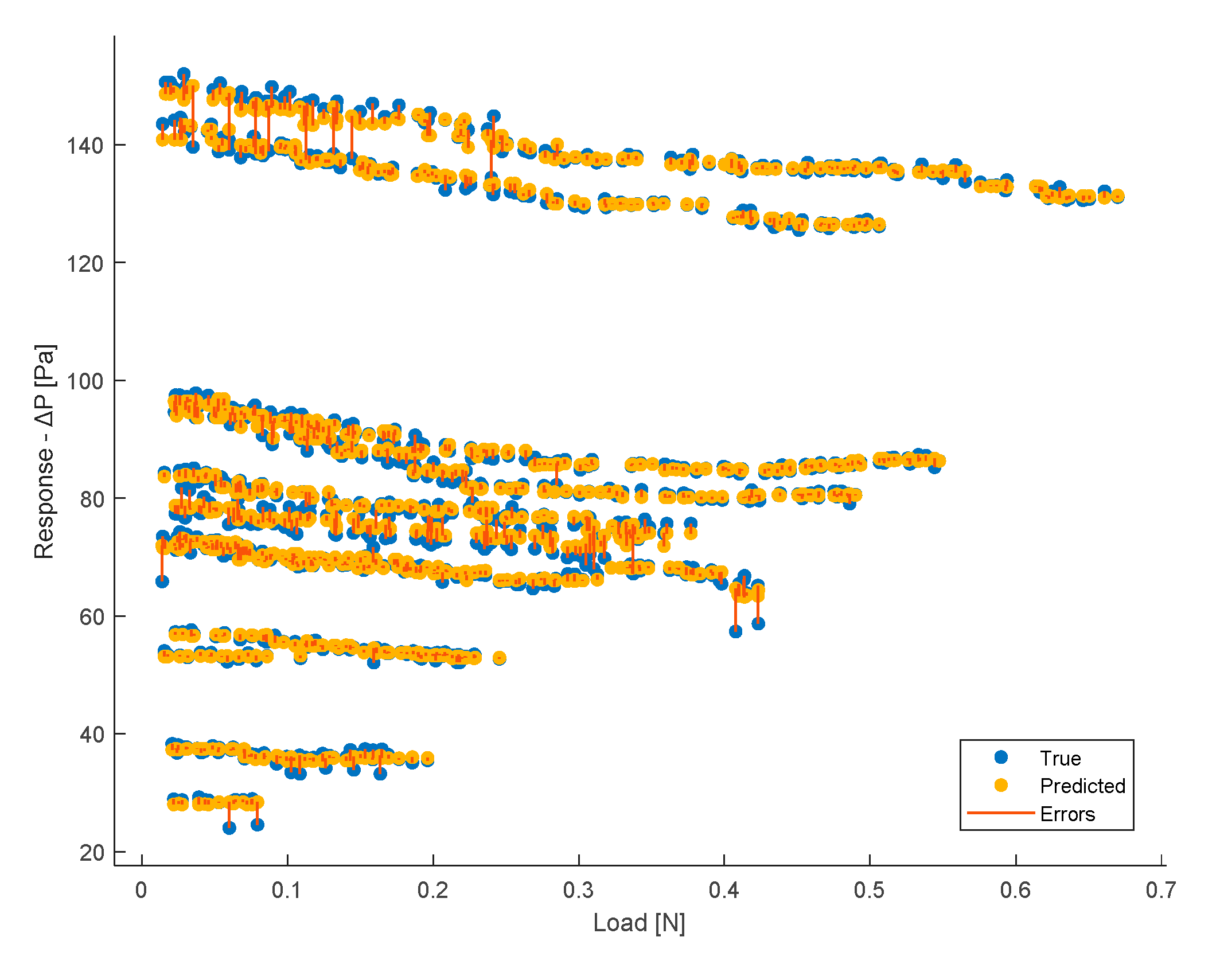
Figure 17.
Comparison between true and predicted responses for each No. PA (a) and PA (yes/no) (b) categories and for each frequency (c) and PA distance (d) values.
Figure 17.
Comparison between true and predicted responses for each No. PA (a) and PA (yes/no) (b) categories and for each frequency (c) and PA distance (d) values.
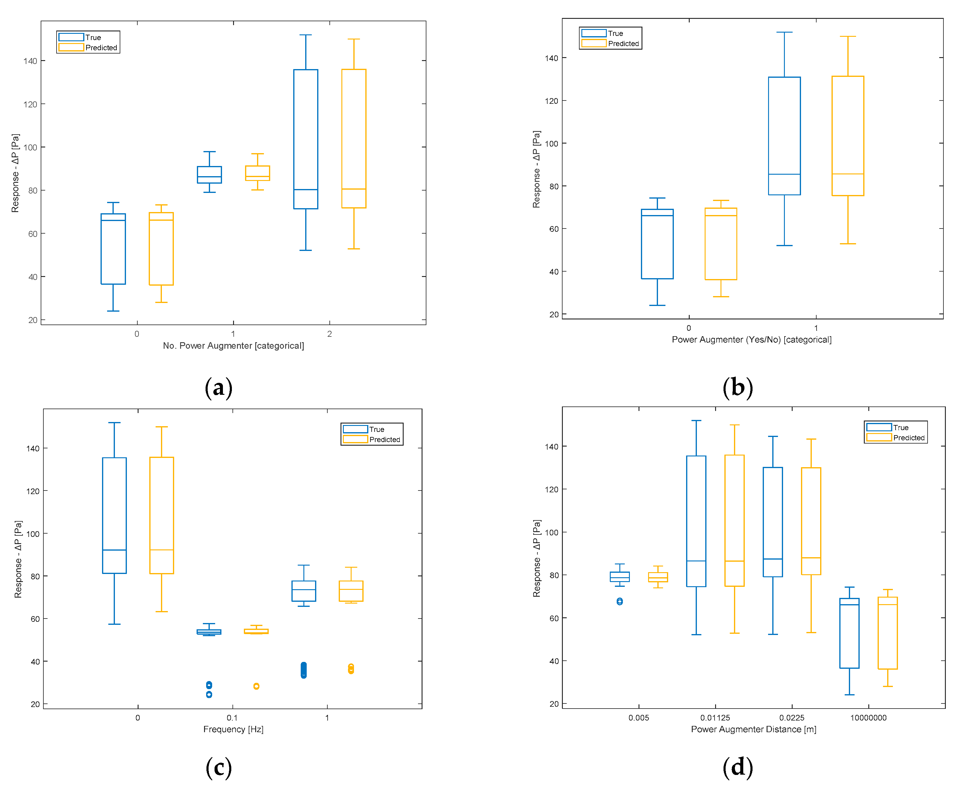
In the previous figures, therefore, the model's responses in terms of ΔP are compared to the true ones. It is possible to observe a sufficient level of closeness, ensuring the goodness of the model as already indicated by the evaluation metrics shown earlier. In the ideal case (R2 = 1, perfect predictions), the box plot of the true responses and that of the predicted ones should be exactly the same. The values being compared are those of ΔP. Therefore, for example in Figure 16, the red line indicating the error depicts exactly the difference between the predicted values and the actual values. As regard the box plot, the central mark denotes the median, while the lower and upper edges of the box represent the 25th and 75th percentiles, respectively. Vertical lines extend from the boxes to the most extreme data points that are not considered outliers. Outliers are individually plotted using the 'o' symbol.
Figure 18(a) displays the correlation between the actual ΔP values (X-axis) and the predicted ones (Y-axis) in the validation phase. The plot is summarized by the R2 coefficient, which, as shown in Table 5, is sufficiently high.
In the ideal case, the predicted ΔP values coincide with the actual ones. In this scenario, all points lie on the line, resulting in an R2 coefficient equal to 1.
Figure 18 (b) displays the residual plot for the 944 observations (the difference between predicted and true values of ΔP). It exhibits a certain symmetry around the axis 0, except for some outliers in the negative part of the plot, and no pattern could be observed. This indicates good performance during the validation phase.
Below, some graphs obtained as a result of the test phase will be shown. Figure 19 (a) displays the correlation plot between the predicted and actual values of ΔP.
In the test phase, there are 100 instances, and from the distribution, it is noticeable how the observations approximate the line of perfect predictions better. This is also evident from the fact that the test R2 is closer to 1 compared to that of validation. This can be interpreted as a good performance of the model, as it has managed to achieve a prediction level comparable to that of validation. This means that the model has generalized well enough to predict new instances with the same level of accuracy. Therefore, hyperparameter optimization has, as expected, reduced the occurrence of overfitting.
Figure 19 (b) displays the residual plot of the test data. Again, apart from an outlier value, the plot exhibits values distributed around zero.
Now, the graphs of partial dependencies of individual features on the response (ΔP) are shown.
The partial dependence plot illustrates the marginal effect that one or two features have on the prediction of a machine learning model [32]. A partial dependence plot can show whether the relationship between the output and a feature is linear, monotonic, or more complex.
In the partial dependence plot of the Load (Figure 20), it can be observed that as the load applied to the turbine increases, the ΔP decreases in a quadratic manner. This can be justified by the fact that as the braking load increases, the turbine generates a progressively lower ΔP.
The partial dependence plot of frequency (Figure 21) shows that for a frequency equal to zero (continuous flow), the ΔP has a high value, while when the flow becomes alternating, there is a rapid decrease in ΔP, which, however, increases as it moves from lower to higher frequencies. However, the highest ΔP value during bidirectional flow remains significantly below the ΔP value at continuous flow (0 Hz).
From the following graph (Figure 22), it is evident that increasing the PA distance and the turbine results in a significant decrease in ΔP from small to large distances (distance values of 106 denote, in practice, the absence of PA).
In the case of categorical features, the partial dependence is obtained by forcing all data instances to belong to the same category. Therefore, a value will be obtained for each class.
Figure 23 displays the partial dependence plot concerning the presence/absence of PA. As can be seen, neither of the two categories prevails over the other in terms of influence on ΔP. Consequently, this feature appears to be irrelevant in determining ΔP. This was partly predictable since, for example, in the previous graph (Figure 22), the PA distance=107 had already been appropriately chosen to represent the absence of PA. Additionally, the feature No. PA encompasses both the absence and presence of PA, providing additional information. However, it was decided to verify this hypothesis. Discarding this feature will not affect the obtained result. It is clarified that what has just been said does not imply that the presence or absence of ramps does not influence ΔP (as evidenced by Figure 22 and Figure 23), but only that it does not make sense to use this type of predictor in the model, as it is correlated with two other predictors.
From the partial dependence plot regarding the No. PA present (Figure 24), it can be observed that the presence of even one ramp has a positive impact on ΔP. With two PA present, ΔP increases significantly compared to the previous case. It is therefore inferred that the presence of PAs, especially two PA, leads to a higher ΔP.
Furthermore, it is possible to extract the importance of the selected features (predictors) in determining the ΔP (as shown in Eq. 18). Figure 25 displays, in descending order, the predictors importance.
The most important features observed during model training are the number of ramps and frequency, which are of comparable importance. A lower weight is associated with the PA distance and the applied load. The feature regarding the presence/absence of PA appears to have no weight. This is consistent with the previous consideration about Figure 23.
Figure 26 shows the counts of the feature used to generate the tree.
The Figure 26 shows a complementary graph of Figure 25. The high counts of splits for the Load [N] denote a great difficult of the algorithm to minimize the cost function (MSE) with this feature, while with the other ones the algorithm needs very low splits count to minimize the MSE. As expected, the binary predictor PA (yes/no) was never utilized to create a split within the tree. An inverse trend between the frequency of a feature's use and its importance is observable (Figure 25). This confirms the general understanding that the most frequently used feature does not always have the greatest influence on determining the output (ΔP).
4. Conclusions
The experimental part of this study aimed to characterize turbine behavior by extracting CP-λ curves from experimental results. These curves represent the relationship between power coefficient (CP) and tip speed ratio (λ). The area under a CP-λ curve gives an estimate of the energy recoverable from wave motion. This area can be increased by either accelerating turbine rotation or improving the power coefficient.
For a flow frequency of 0 Hz, results show that with a unidirectional flow, the greatest improvement occurs with 1-PA configurations, particularly as the proximity of the PA to the turbine increases. However, 2-PA configurations do not improve power due to downwind PA disturbance, though they do increase tip speed ratio.
For a frequency of 0.1 Hz, adding 2 PAn significantly increases the power coefficient at a distance of d/8, making it the optimal configuration among those tested.
Similarly to the 0.1 Hz condition, when f=1 Hz the best performance is achieved with 2 PA at d/8 from the turbine, though the improvements in power coefficient and tip speed ratio compared to the no-PA case are not as substantial.
Regarding the development of the predictive model, it was observed that among the features used, the greatest importance in determining ΔP is attributable to No. PA. Another feature of comparable importance is the fluid flow frequency. It was also noted that one of the selected features, the presence of PA (yes/no), has no impact on determining the output as it is inherently correlated with two other features (PA distance and No. PA). Therefore, it does not affect the model training and can be excluded. Obtaining a predictive model opens up the possibility of conducting further tests without the need to resort to the physical system, allowing for the evaluation of different scenarios. As future developments, training the model under additional conditions could be considered, always subject to obtaining experimental data, such as at different speeds.
Author Contributions
For research articles with several authors, a short paragraph specifying their individual contributions must be provided. The following statements should be used “Conceptualization, E.B., S.B., M.C., and F.S.; methodology, E.B., S.B., M.C., and F.S; software, E.B.; validation, E.B., M.C. and F.S.; formal analysis, E.B. and M.C.; investigation, S.B. and F.S.; resources, S.B.; data curation, E.B., G.B., and M.C.; writing—original draft preparation, E.B. and M.C.; writing—review and editing, F.S.; visualization, E.B. and M.C.; supervision, F.S.; project administration, F.S.; funding acquisition, S.B. All authors have read and agreed to the published version of the manuscript.”.
Informed Consent Statement
Not applicable.
Data Availability Statement
Data available upon request.
Conflicts of Interest
The authors declare no conflicts of interest.
References
- Lamb, W.F.; Wiedmann, T.; Pongratz, J.; Andrew, R.; Crippa, M.; Olivier, J.G.J.; Wiedenhofer, D.; Mattioli, G.; Khourdajie, A. Al; House, J.; et al. A Review of Trends and Drivers of Greenhouse Gas Emissions by Sector from 1990 to 2018. Environmental Research Letters 2021, 16, 073005. [Google Scholar] [CrossRef]
- Lunde Hermansson, A.; Hassellöv, I.M.; Moldanová, J.; Ytreberg, E. Comparing Emissions of Polyaromatic Hydrocarbons and Metals from Marine Fuels and Scrubbers. Transp Res D Transp Environ 2021, 97, 102912. [Google Scholar] [CrossRef]
- Cucinotta, F.; Barberi, E.; Salmeri, F. A Review on Navigating Sustainable Naval Design: LCA and Innovations in Energy and Fuel Choices. Journal of Marine Science and Engineering 2024, Vol. 12, Page 520 2024, 12, 520. [Google Scholar] [CrossRef]
- Yusuf, A.A.; Yusuf, D.A.; Jie, Z.; Bello, T.Y.; Tambaya, M.; Abdullahi, B.; Muhammed-Dabo, I.A.; Yahuza, I.; Dandakouta, H. Influence of Waste Oil-Biodiesel on Toxic Pollutants from Marine Engine Coupled with Emission Reduction Measures at Various Loads. Atmos Pollut Res 2022, 13, 101258. [Google Scholar] [CrossRef]
- Cucinotta, F.; Raffaele, M.; Salmeri, F. A Well-to-Wheel Comparative Life Cycle Assessment Between Full Electric and Traditional Petrol Engines in the European Context. Lecture Notes in Mechanical Engineering 2021, 188–193. [Google Scholar] [CrossRef]
- Bilgili, L. Comparative Assessment of Alternative Marine Fuels in Life Cycle Perspective. Renewable and Sustainable Energy Reviews 2021, 144, 110985. [Google Scholar] [CrossRef]
- Rial, R.C. Biofuels versus Climate Change: Exploring Potentials and Challenges in the Energy Transition. Renewable and Sustainable Energy Reviews 2024, 196, 114369. [Google Scholar] [CrossRef]
- Garg, R.; Sabouni, R.; Ahmadipour, M. From Waste to Fuel: Challenging Aspects in Sustainable Biodiesel Production from Lignocellulosic Biomass Feedstocks and Role of Metal Organic Framework as Innovative Heterogeneous Catalysts. Ind Crops Prod 2023, 206, 117554. [Google Scholar] [CrossRef]
- Ershov, M.A.; Savelenko, V.D.; Makhova, U.A.; Makhmudova, A.E.; Zuikov, A. V.; Kapustin, V.M.; Abdellatief, T.M.M.; Burov, N.O.; Geng, T.; Abdelkareem, M.A.; et al. Current Challenge and Innovative Progress for Producing HVO and FAME Biodiesel Fuels and Their Applications. Waste Biomass Valorization 2023, 14, 505–521. [Google Scholar] [CrossRef]
- Huang, W.; Zulkifli, M.Y. Bin; Chai, M.; Lin, R.; Wang, J.; Chen, Y.; Chen, V.; Hou, J. Recent Advances in Enzymatic Biofuel Cells Enabled by Innovative Materials and Techniques. Exploration 2023, 3, 20220145. [Google Scholar] [CrossRef]
- Zhang, L.; Jia, C.; Bai, F.; Wang, W.; An, S.; Zhao, K.; Li, Z.; Li, J.; Sun, H. A Comprehensive Review of the Promising Clean Energy Carrier: Hydrogen Production, Transportation, Storage, and Utilization (HPTSU) Technologies. Fuel 2024, 355, 129455. [Google Scholar] [CrossRef]
- Prestipino, M.; Salmeri, F.; Cucinotta, F.; Galvagno, A. Thermodynamic and Environmental Sustainability Analysis of Electricity Production from an Integrated Cogeneration System Based on Residual Biomass: A Life Cycle Approach. Appl Energy 2021, 295, 117054. [Google Scholar] [CrossRef]
- Puleio, F.; Rizzo, G.; Nicita, F.; Giudice, F. Lo; Tamà, C.; Marenzi, G.; Centofanti, A.; Raffaele, M.; Santonocito, D.; Risitano, G. Chemical and Mechanical Roughening Treatments of a Supra-Nano Composite Resin Surface: SEM and Topographic Analysis. Applied Sciences (Switzerland) 2020, 10. [Google Scholar] [CrossRef]
- Di Bella, G.; Alderucci, T.; Salmeri, F.; Cucinotta, F. Integrating the Sustainability Aspects into the Risk Analysis for the Manufacturing of Dissimilar Aluminium/Steel Friction Stir Welded Single Lap Joints Used in Marine Applications through a Life Cycle Assessment. Sustainable Futures 2022, 4, 100101. [Google Scholar] [CrossRef]
- Xu, C.; Huang, Z. Three-Dimensional CFD Simulation of a Circular OWC with a Nonlinear Power-Takeoff: Model Validation and a Discussion on Resonant Sloshing inside the Pneumatic Chamber. Ocean Engineering 2019, 176, 184–198. [Google Scholar] [CrossRef]
- Ning, D.Z.; Wang, R.Q.; Zou, Q.P.; Teng, B. An Experimental Investigation of Hydrodynamics of a Fixed OWC Wave Energy Converter. Appl Energy 2016, 168, 636–648. [Google Scholar] [CrossRef]
- Devin, D.; Halim, L.; Arthaya, B.M.; Chandra, J.; Devin, D.; Halim, L.; Arthaya, B.M.; Chandra, J. Design and CFD Simulation of Guide Vane for Multistage Savonius Wind Turbine. Journal of Mechatronics, Electrical Power, and Vehicular Technology 2023, 14, 186–197. [Google Scholar] [CrossRef]
- Mauro, S.; Brusca, S.; Lanzafame, R.; Messina, M. CFD Modeling of a Ducted Savonius Wind Turbine for the Evaluation of the Blockage Effects on Rotor Performance. Renew Energy 2019, 141, 28–39. [Google Scholar] [CrossRef]
- Zaki, M.B.; Al-Quraishi, Y.; Sarip, S.; Fairul Izzat, M. TAGUCHI OPTIMIZATION OF WATER SAVONIUS TURBINE FOR LOW-VELOCITY INLETS USING CFD APPROACH. Journal of Energy and Safety Technology (JEST) 2023, 6, 1–7. [Google Scholar] [CrossRef]
- Chillemi, M.; Cucinotta, F.; Passeri, D.; Scappaticci, L.; Sfravara, F. CFD-Driven Shape Optimization of a Racing Motorcycle. Lecture Notes in Mechanical Engineering 2024, 488–496. [Google Scholar] [CrossRef]
- Cucinotta, F.; Raffaele, M.; Salmeri, F. A Topology Optimization Method for Stochastic Lattice Structures. Lecture Notes in Mechanical Engineering 2021, 235–240. [Google Scholar] [CrossRef]
- Brusca, S.; Galvagno, A.; Mauro, S.; Messina, M.; Lanzafame, R. Bell-Metha Power Augmented Savonius Turbine as Take-off in OWC Systems. J Phys Conf Ser 2023, 2648, 012015. [Google Scholar] [CrossRef]
- Saikot, M.M.H.; Rahman, M.; Hosen, M.A.; Ajwad, W.; Jamil, M.F.; Islam, M.Q. Savonius Wind Turbine Performance Comparison with One and Two Porous Deflectors: A CFD Study. Flow Turbul Combust 2023, 111, 1227–1251. [Google Scholar] [CrossRef]
- Aboujaoude, H.; Bogard, F.; Beaumont, F.; Murer, S.; Polidori, G. Aerodynamic Performance Enhancement of an Axisymmetric Deflector Applied to Savonius Wind Turbine Using Novel Transient 3D CFD Simulation Techniques. Energies 2023, Vol. 16, Page 909 2023, 16, 909. [Google Scholar] [CrossRef]
- Udousoro, I.C. Machine Learning:A Review. Semiconductor Science and Information Devices 2020, 2. [Google Scholar] [CrossRef]
- Jordan, M.I.; Mitchell, T.M. Machine Learning: Trends, Perspectives, and Prospects. Science (1979) 2015, 349, 255–260. [Google Scholar] [CrossRef]
- Marquis, P.; Papini, O.; Prade, H. Elements for a History of Artificial Intelligence. In A Guided Tour of Artificial Intelligence Research; Springer International Publishing: Cham, 2020; pp. 1–43. [Google Scholar]
- Muggleton, S. Alan Turing and the Development of Artificial Intelligence. AI Communications 2014, 27, 3–10. [Google Scholar] [CrossRef]
- Géron, A. Hands-On Machine Learning with Scikit-Learn, Keras, and TensorFlow: Concepts, Tools, and Techniques to Build Intelligent Systems; 2nd Edition.; O’Reilly, 2019.
- Mantovani, R.G.; Horvath, T.; Cerri, R.; Vanschoren, J.; de Carvalho, A.C.P.L.F. Hyper-Parameter Tuning of a Decision Tree Induction Algorithm. In Proceedings of the 2016 5th Brazilian Conference on Intelligent Systems (BRACIS); October 2016; pp. 37–42. [Google Scholar]
- Yang, L.; Shami, A. On Hyperparameter Optimization of Machine Learning Algorithms: Theory and Practice. Neurocomputing 2020, 415, 295–316. [Google Scholar] [CrossRef]
- Friedman, J.H. Greedy Function Approximation: A Gradient Boosting Machine. The Annals of Statistics 2001, 29. [Google Scholar] [CrossRef]
Figure 1.
Test tube in the UNIME lab.
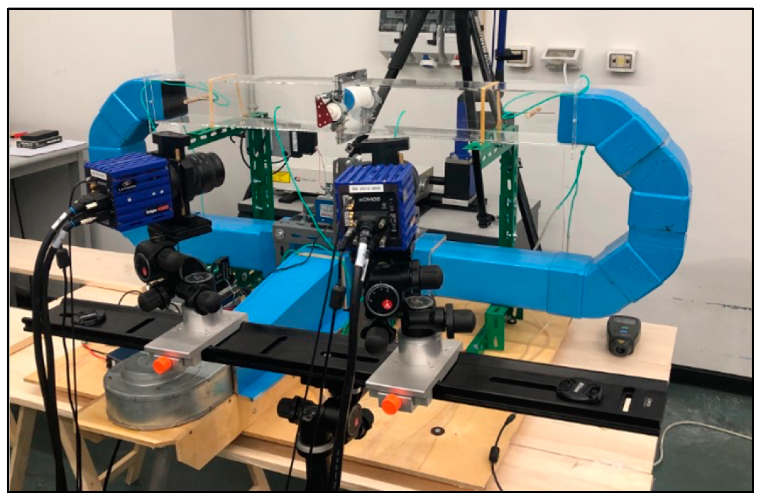
Figure 2.
Layout of the test tube.
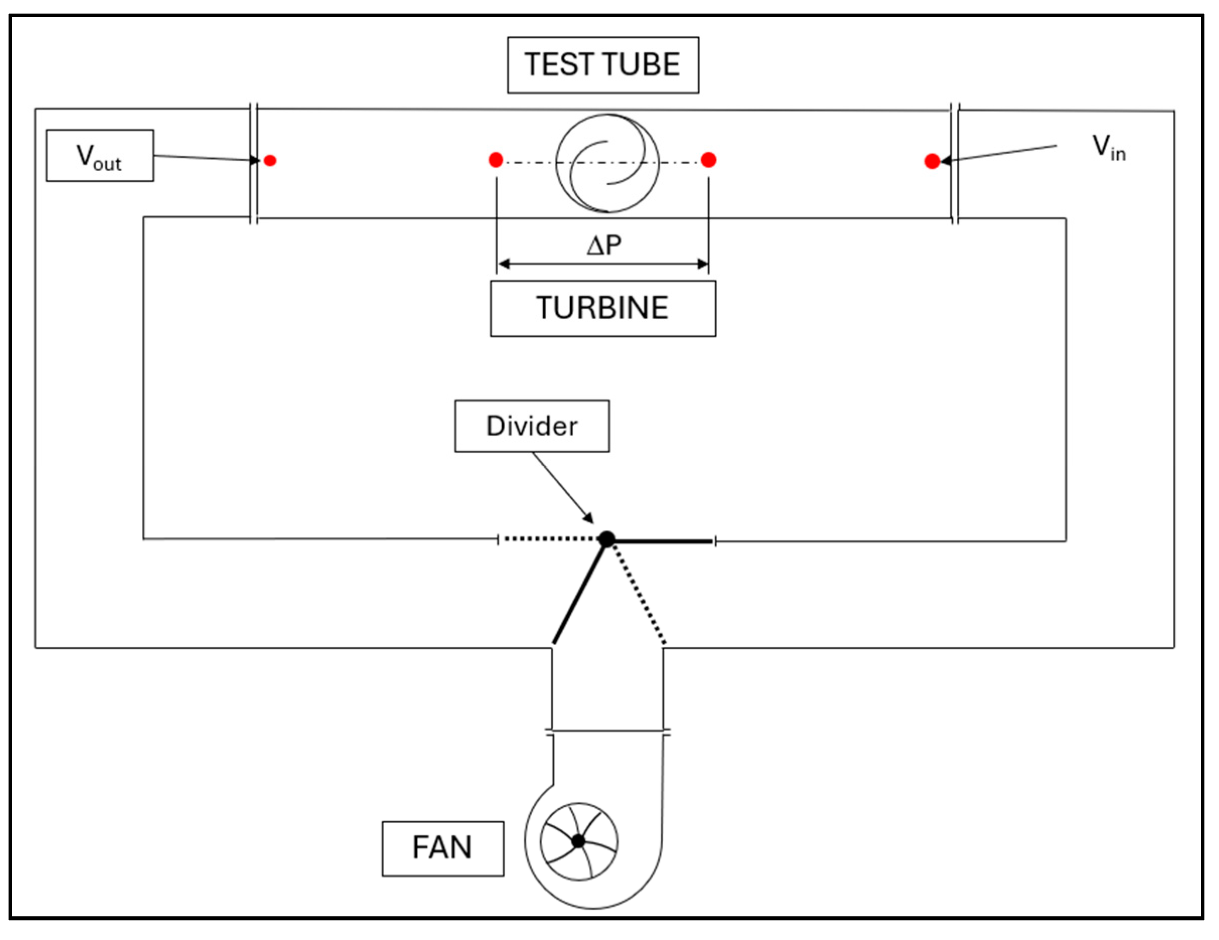
Figure 3.
Mobile diverter.
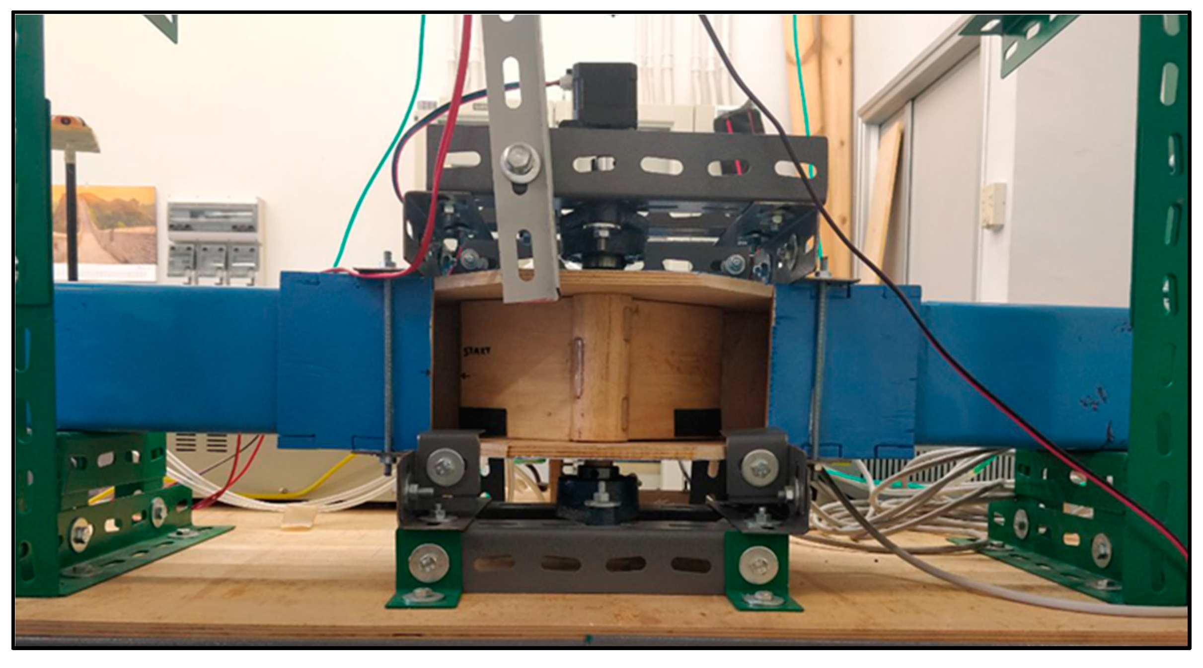
Figure 4.
Power augmenter dimensions.
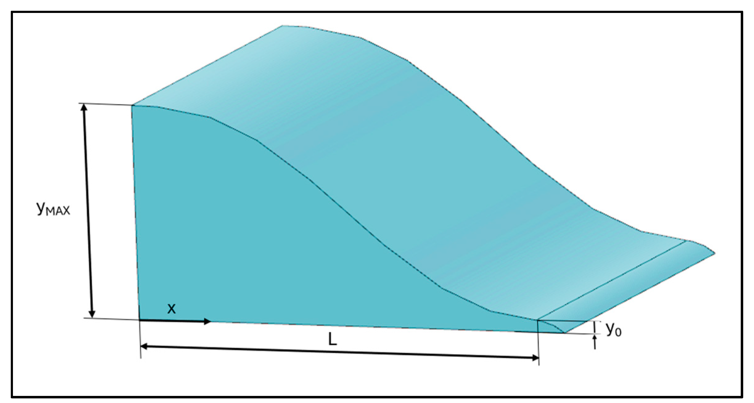
Figure 5.
Example of upwind power augmenter positioning (f=0 Hz).

Figure 6.
Connections between measurement devices and control systems.
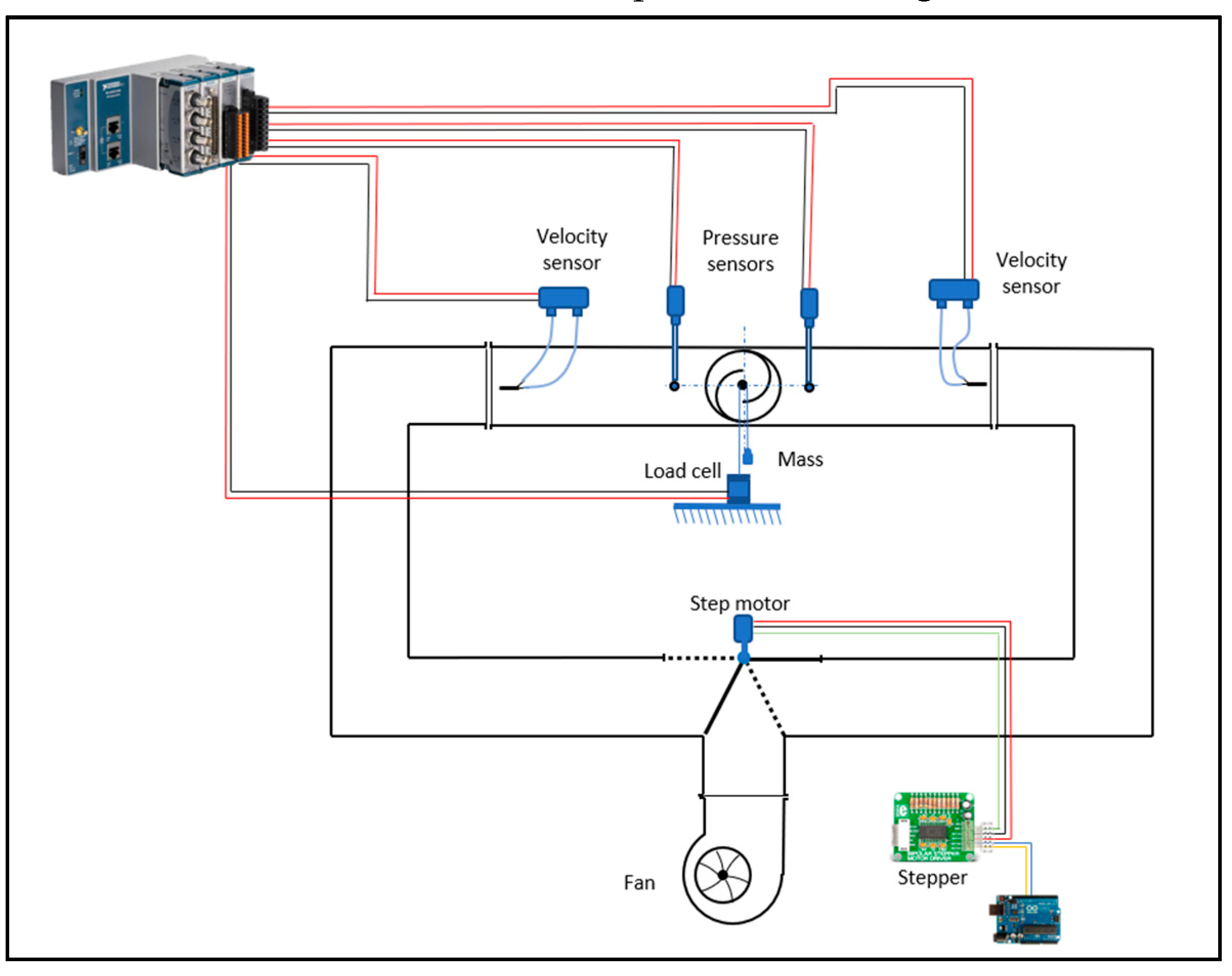
Figure 7.
Torque measurement system.
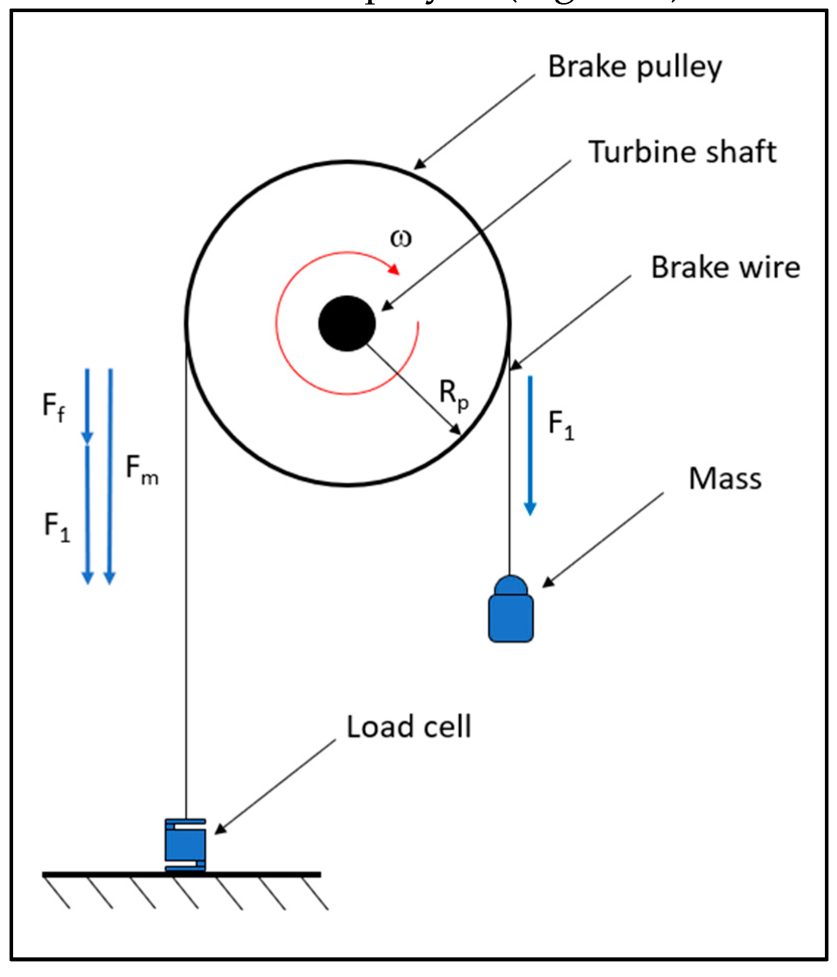
Figure 8.
Schematization of a decision tree.
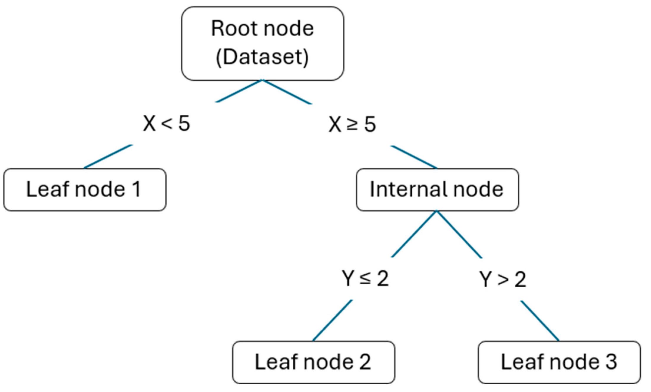
Figure 9.
Example of experimental points curve fitting.
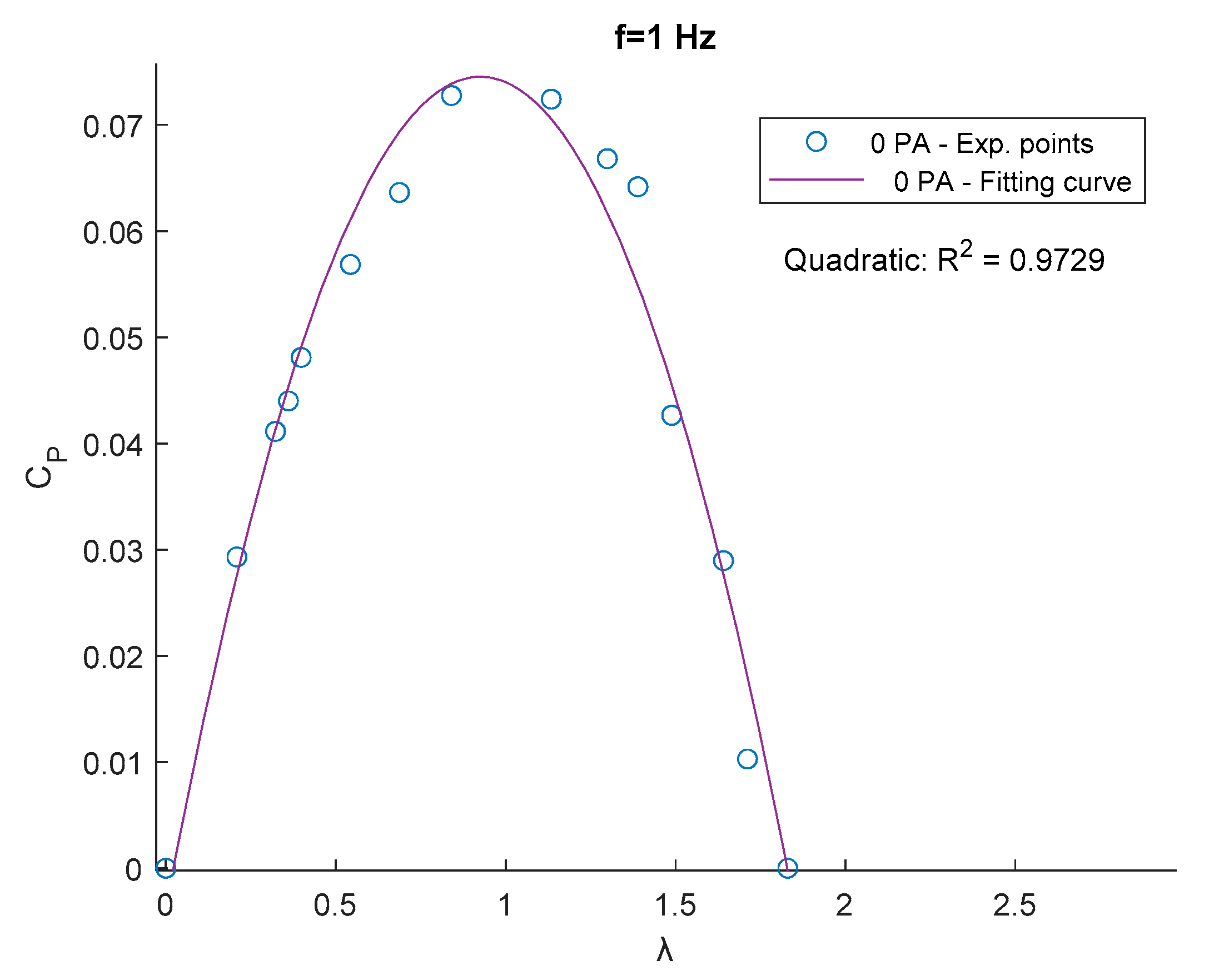
Figure 10.
CP-λ curves for f=0 Hz.
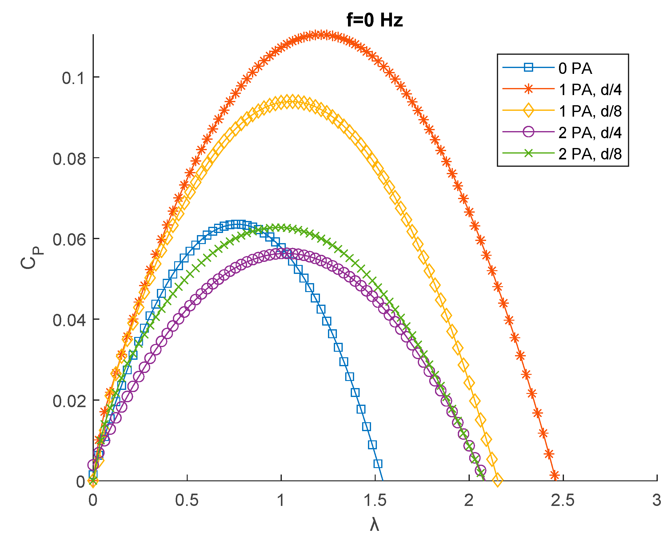
Figure 11.
CP-λ curves for f=0.1 Hz.
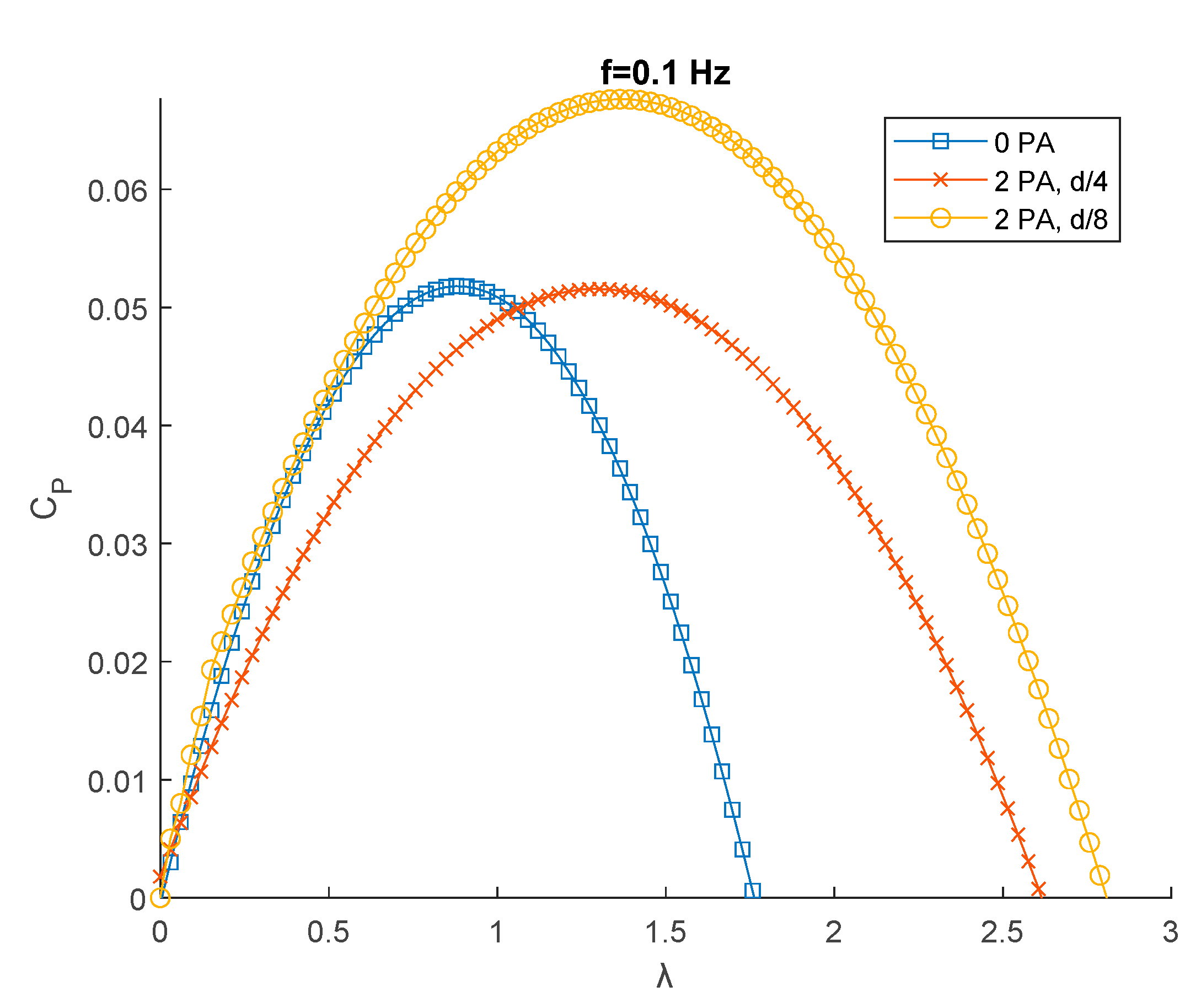
Figure 12.
CP-λ curves for f=0.1 Hz.
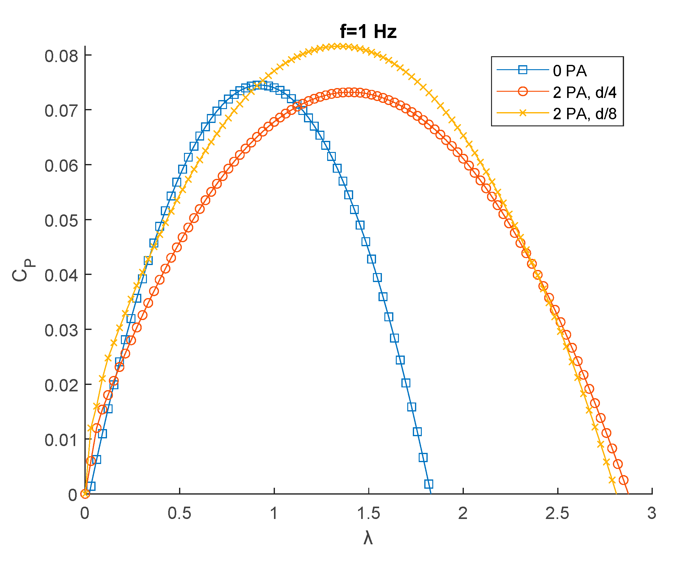
Figure 13.
Comparison of area values between different configurations.
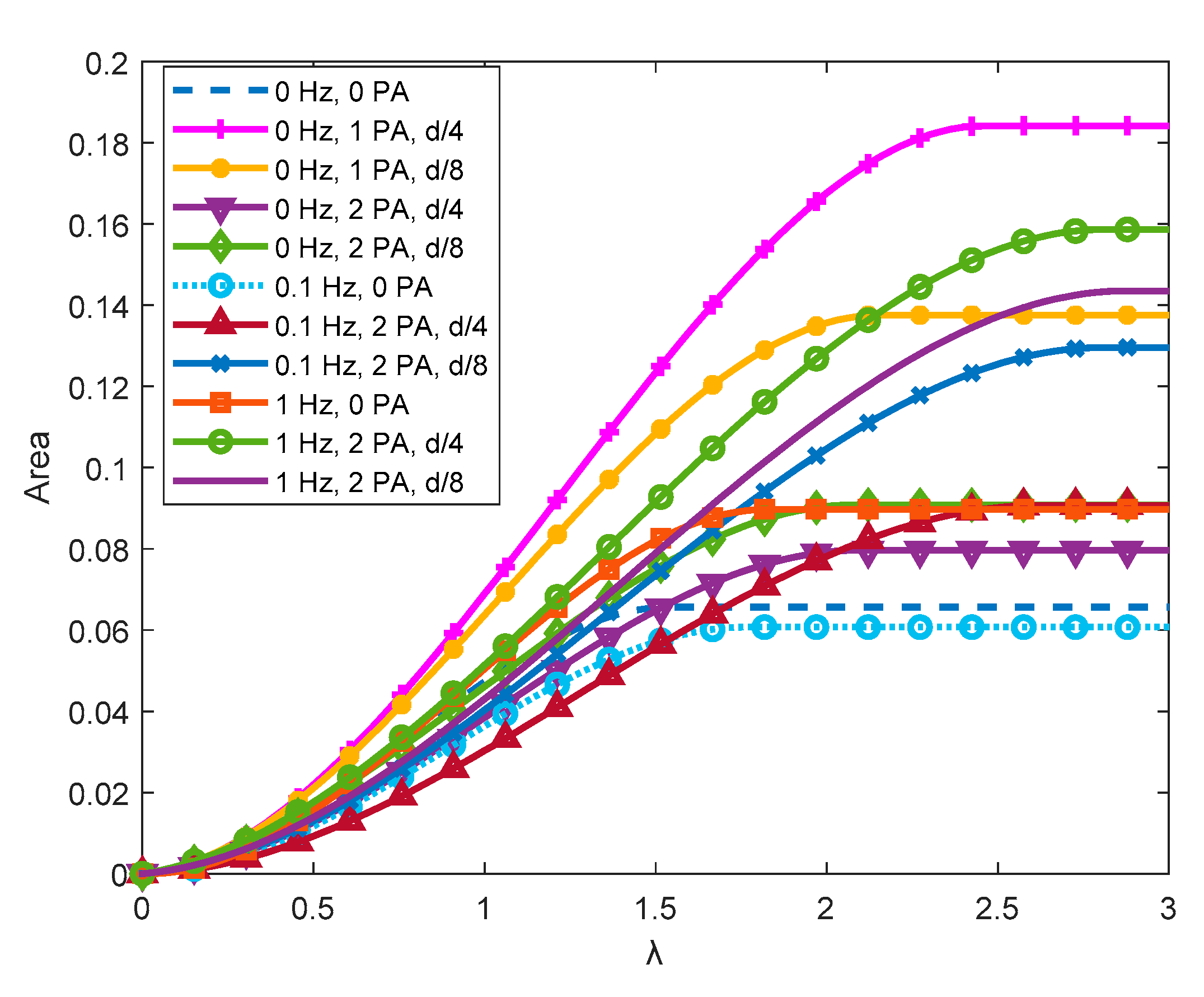
Figure 14.
Minimum MSE values during the iterations and best point hyperparameters.
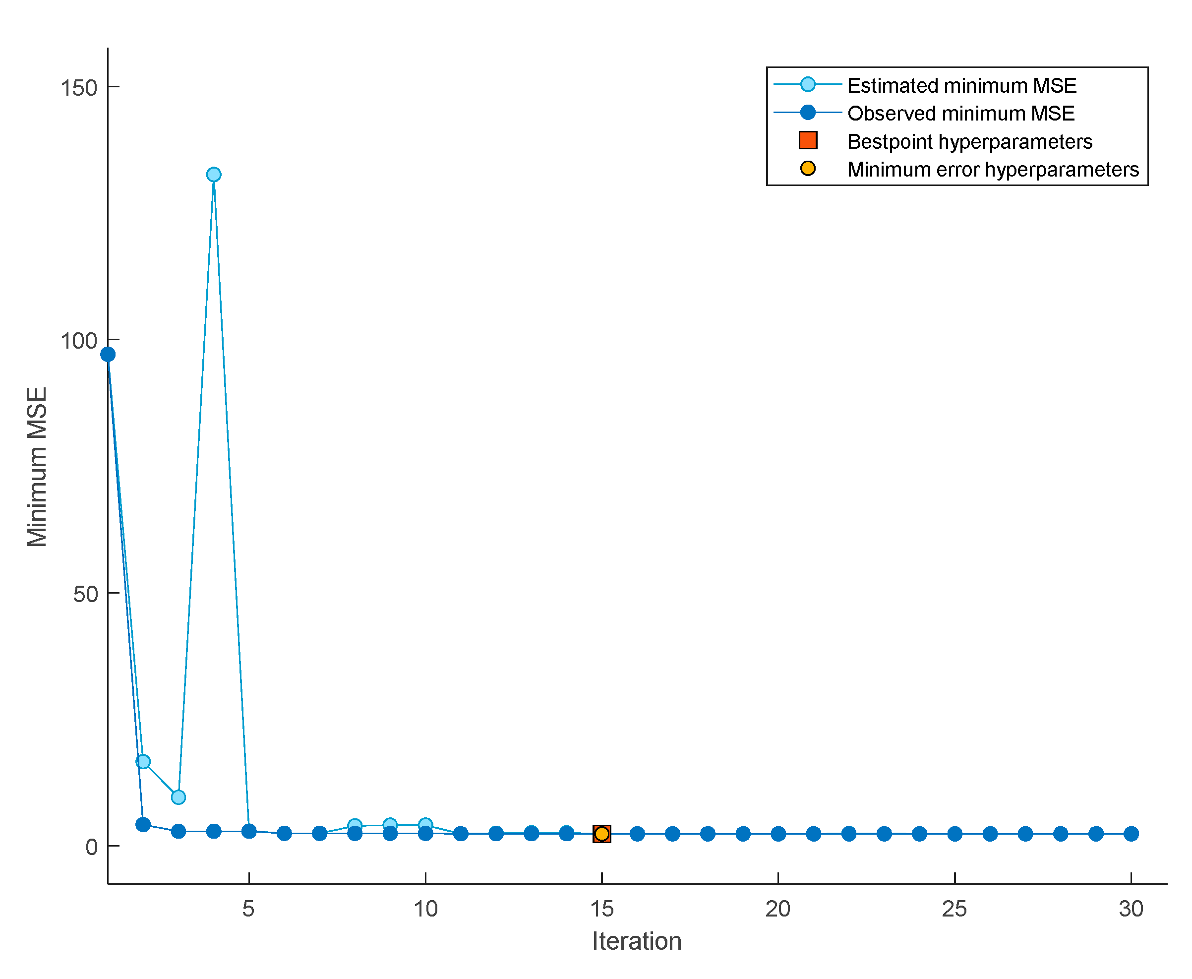
Figure 15.
Comparison between true and predicted responses for each instance.
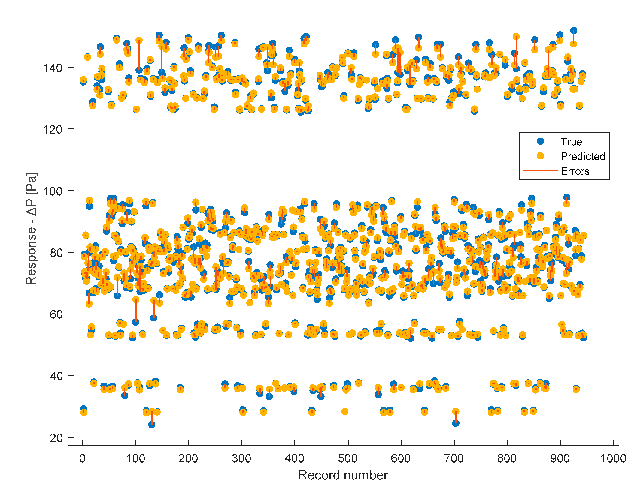
Figure 18.
Prediction accuracy (R2 = 0.99767 ) (a) and residual plot (b) of the validation phase.
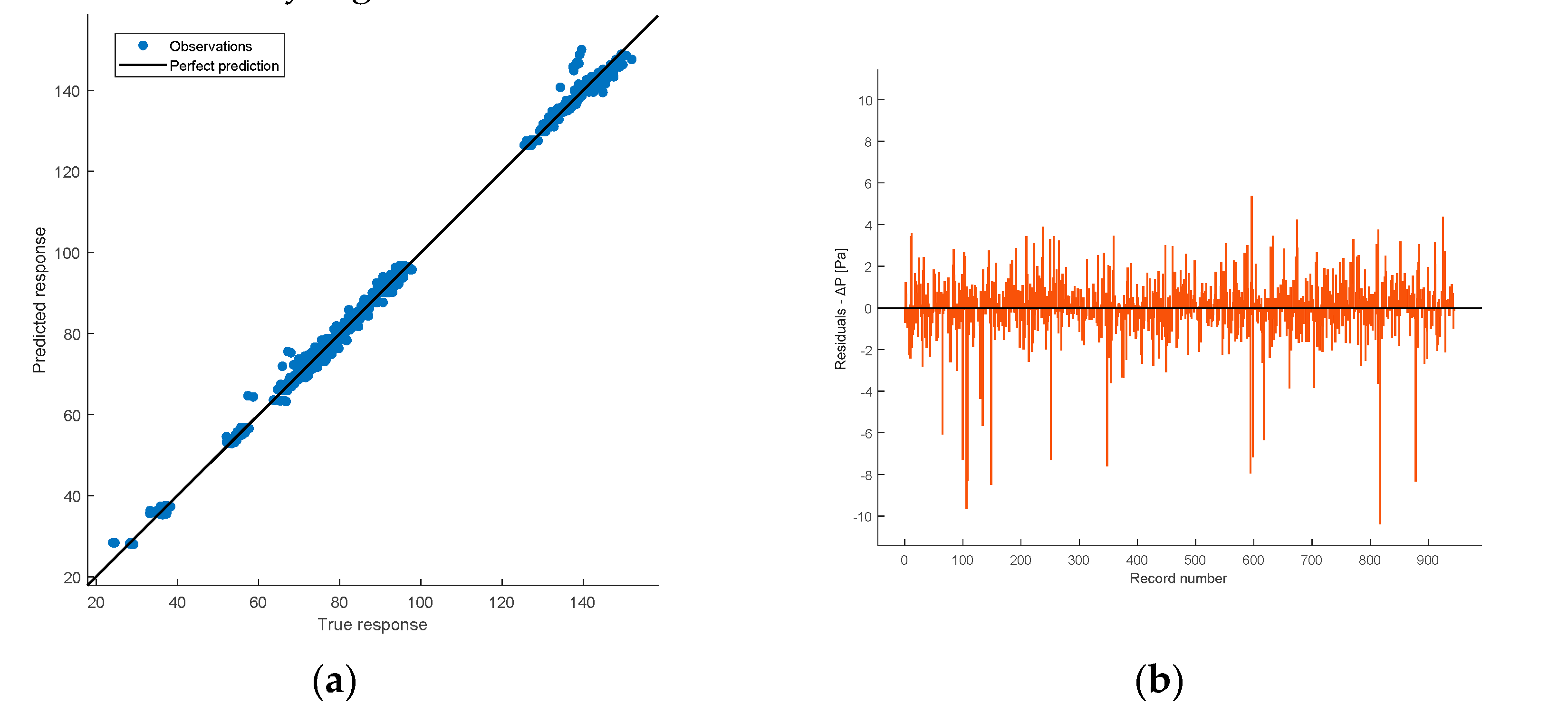
Figure 19.
Prediction accuracy (R2 = 0.99801) (a) and residual plot (b) of the test phase.
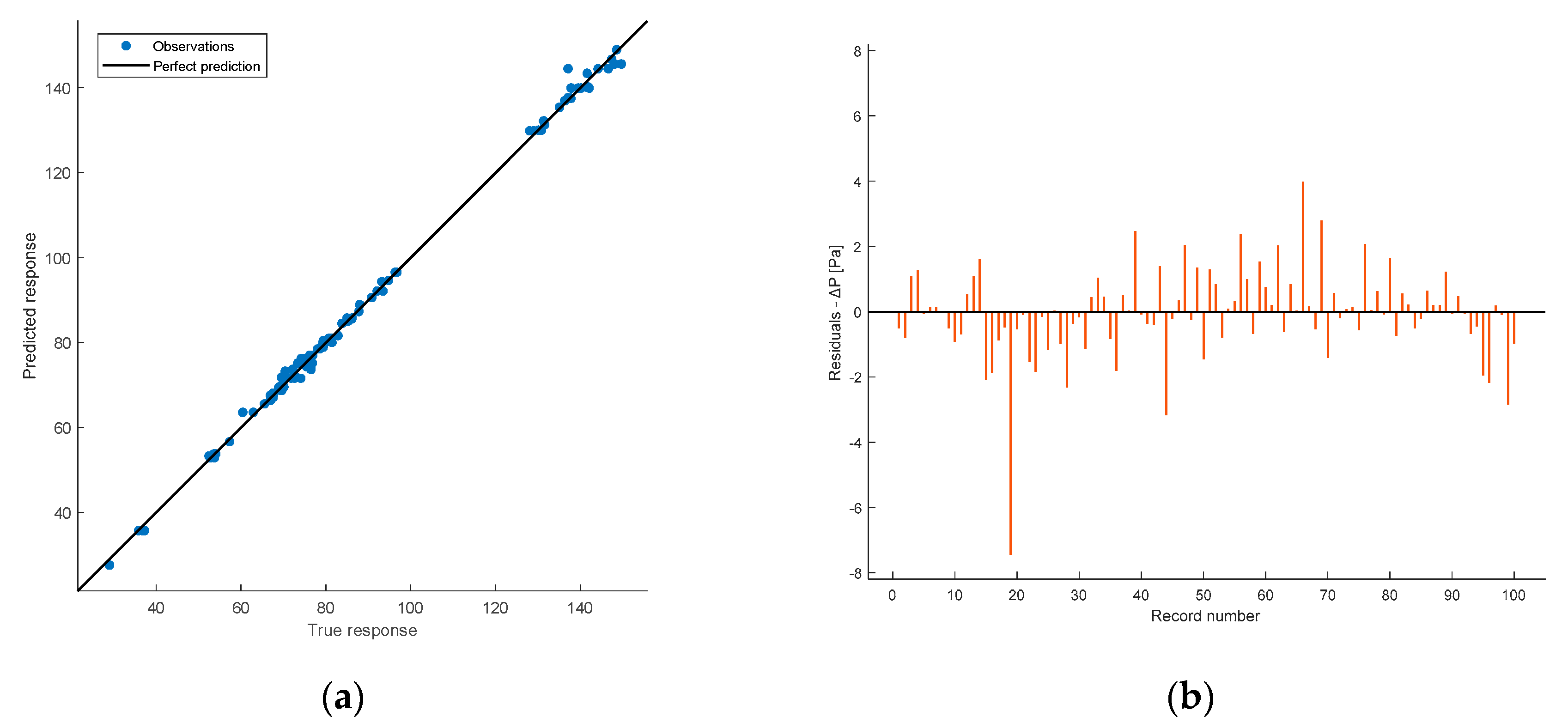
Figure 20.
Partial dependence plot of the Load.
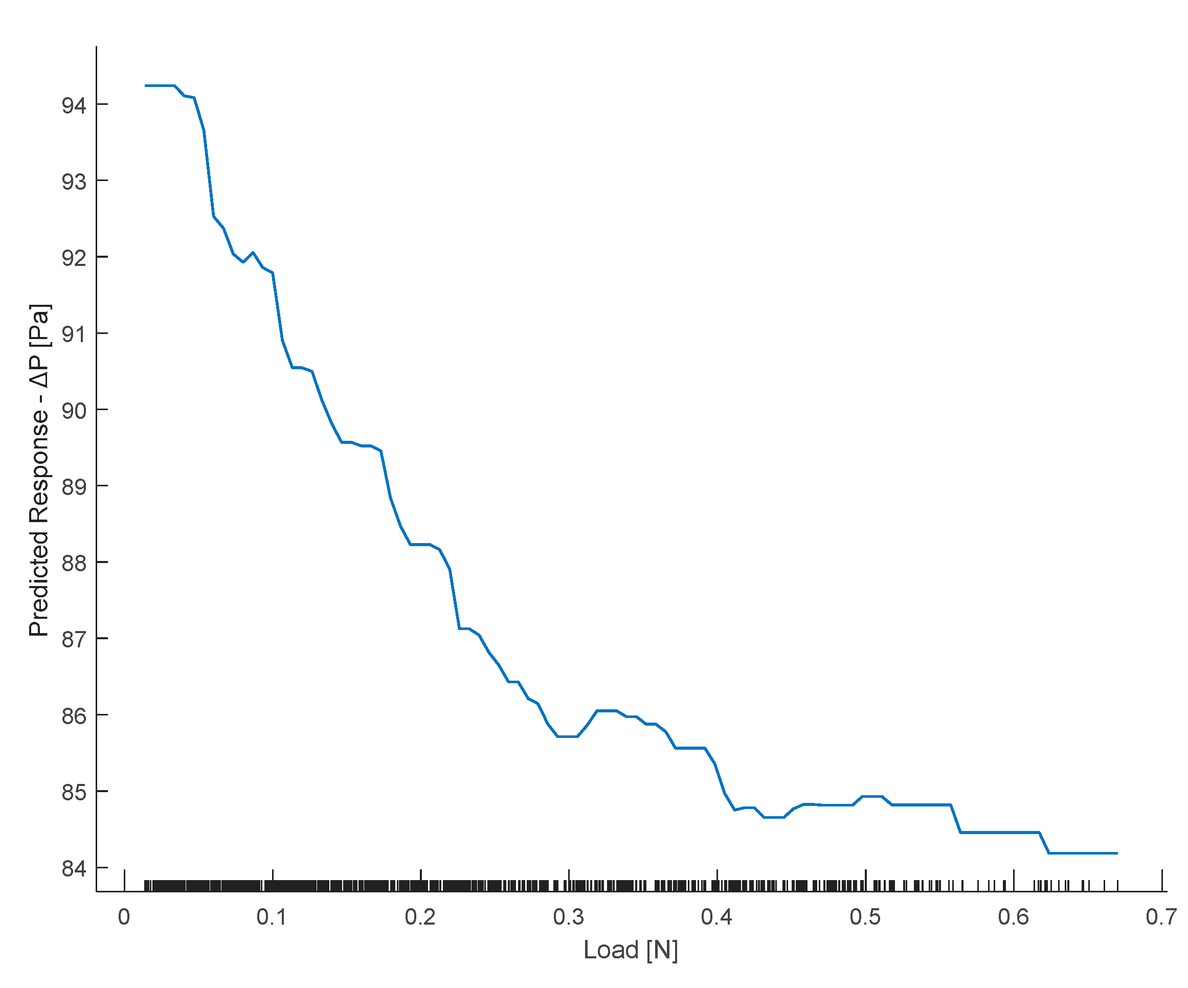
Figure 21.
Partial dependence plot of the Frequency.
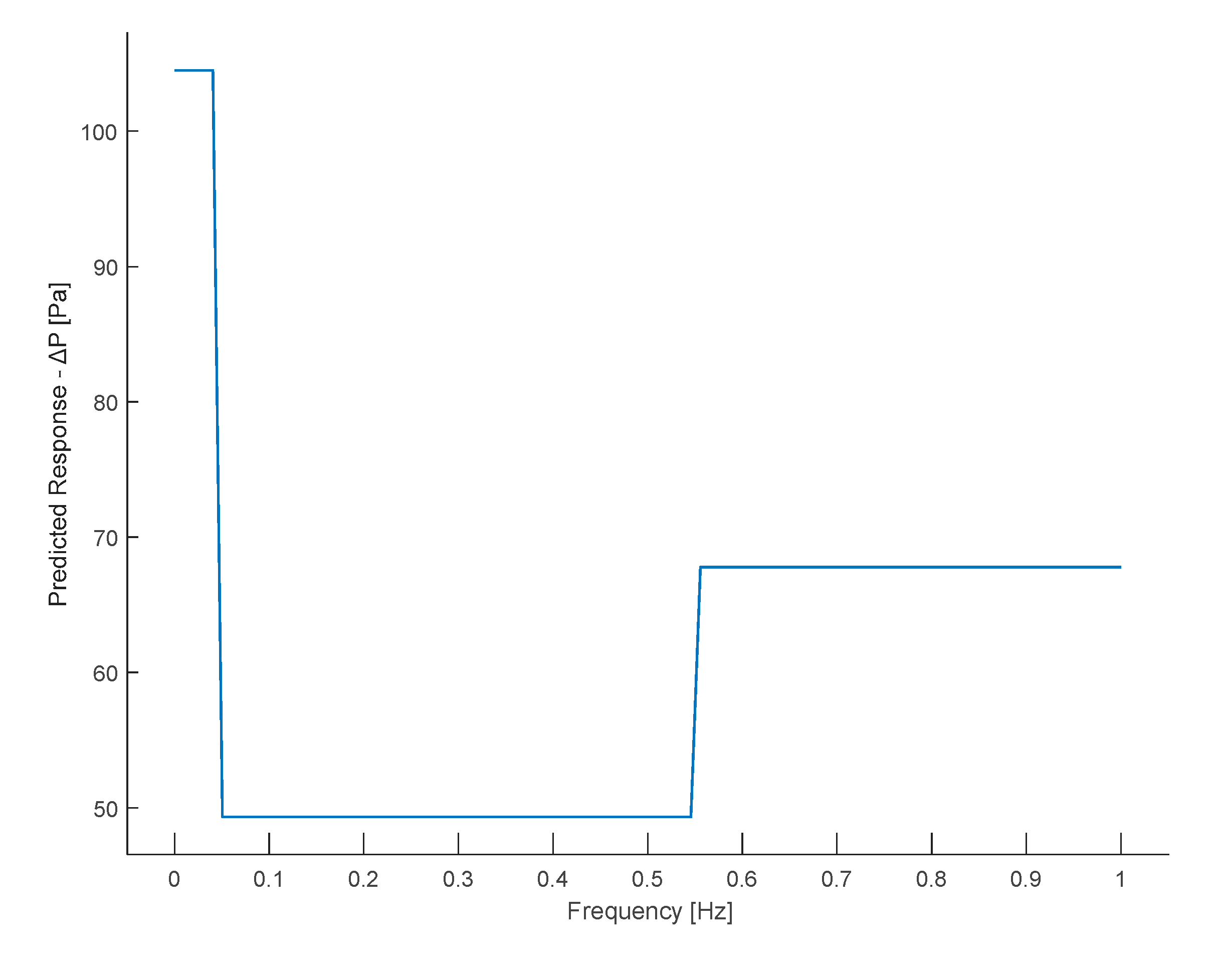
Figure 22.
Partial dependence plot of the PA distance.
Figure 23.
Partial dependence plot of the PA (yes/no).
Figure 24.
Partial dependence plot of the No. PA.
Figure 25.
Predictor importance bar plot.
Figure 26.
Count of the features used to split nodes.
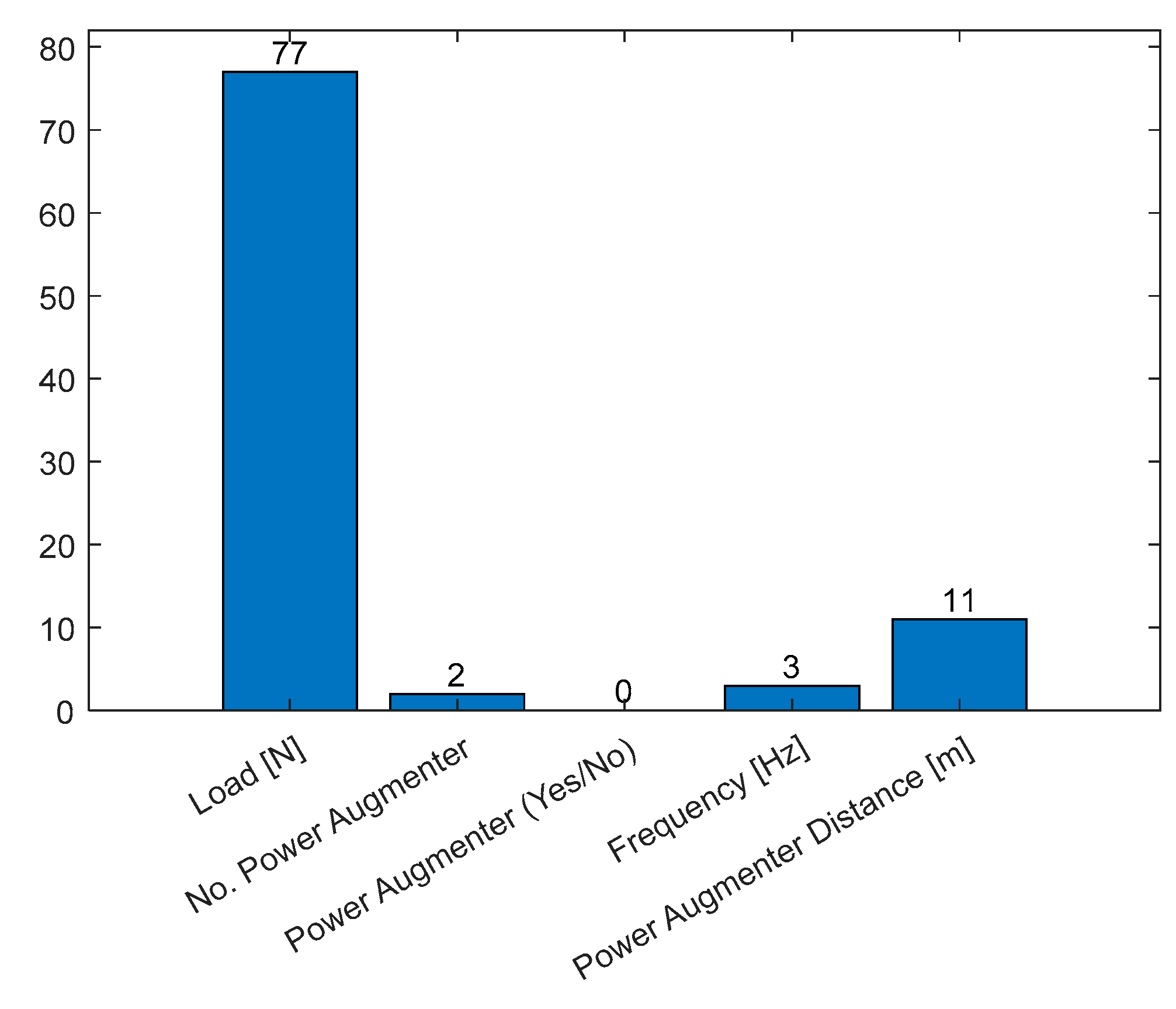

Table 1.
Turbine characteristics.
| Parameter | Symbol | Value |
|---|---|---|
| Diameter [mm] | Dturbine | 90 |
| Height [mm] | h | 90 |
| Overlap Ratio | OR | 1/3 |
| Aspect Ratio | AR | 1 |
| Spacing Ratio | SR | 0 |
| Axis diameter [mm] | AD | 10 |
| Axis length [mm] | AL | 60 |
| Weight [kg] | W | 0.635 |
Table 2.
Tested configuration.
| Configuration number | Number of PA | PA distance | Frequency [Hz] |
|---|---|---|---|
| 1 | 0 | 0 | |
| 2 | 0 | 0.1 | |
| 3 | 0 | 1 | |
| 4 | 1 | D/4 | 0 |
| 5 | 1 | D/8 | 0 |
| 6 | 2 | D/4 | 0 |
| 7 | 2 | D/4 | 0.1 |
| 8 | 2 | D/4 | 1 |
| 9 | 2 | D/8 | 0 |
| 10 | 2 | D/8 | 0.1 |
| 11 | 2 | D/8 | 1 |
Table 3.
Setup variables with description and range of values.
| Load [N] | No. PA | PA (Presence/Absence) | Fan Frequency [Hz] | Distance PA – Turbine [mm] | |
|---|---|---|---|---|---|
| 0.0138 – 0.6701 (continuous) |
0, 1, 2(categorical) | 1,0 (categorical) | 0 – 1(continuous) | 0.0117 – 107(continuous) |
Table 4.
Datasets and number of instances.
| Dataset | No. Instances |
|---|---|
| Total | 1,044 |
| Train/Validation | 944 |
| Test | 100 |
Table 5.
Performance (validation and test) of the trained ML model.
| MSE | RMSE | R2 | MAE | |
|---|---|---|---|---|
| Validation | 2.3773 | 1.5419 | 0.99767 | 1.0226 |
| Test | 1.9539 | 1.3978 | 0.99801 | 0.93791 |
Table 6.
Best combination of the hyperparameters selected.
| Hyperparameter | Value |
|---|---|
| Minimum Leaf Size | 8 |
| Maximum No. Split | 943 |
| Minimum Parent Size | 16 |
Disclaimer/Publisher’s Note: The statements, opinions and data contained in all publications are solely those of the individual author(s) and contributor(s) and not of MDPI and/or the editor(s). MDPI and/or the editor(s) disclaim responsibility for any injury to people or property resulting from any ideas, methods, instructions or products referred to in the content. |
© 2024 by the authors. Licensee MDPI, Basel, Switzerland. This article is an open access article distributed under the terms and conditions of the Creative Commons Attribution (CC BY) license (http://creativecommons.org/licenses/by/4.0/).
Copyright: This open access article is published under a Creative Commons CC BY 4.0 license, which permit the free download, distribution, and reuse, provided that the author and preprint are cited in any reuse.


