Predictive Analytics Performance on Oil and Gas: A Significant Review

Enhancing the management and monitoring of oil and gas processes demands developing precise predictive analytics techniques. Over the past two years, oil and its prediction have advanced significantly using conventional and modern Machine Learning techniques. Several review articles detail the developments in predictive maintenance and technical and non-technical aspects of influencing the uptake of big data. The absence of references for machine learning techniques impacts the effective optimization of predictive analytics in the oil and gas sector. This review paper offers readers thorough information on the latest machine learning methods utilized in this industry's predictive analytical modelling. The review covers forms of Machine Learning techniques used in predictive analytic modelling from 2021 to 2023 (91 articles). It provides an overview of the details of the papers that were reviewed, comprising of the model’s categories, the data's temporality, field, and name, the dataset's type, predictive analytics (classification or clustering or prediction), the models' input and output parameters, performance metrics, optimal model, and benefits and its drawbacks. Additionally, suggestions for future research directions are provided to raise the potential of the associated knowledge and increase the accuracy of oil and gas predictive analytics models.

Keywords:

classification

;

clustering

;

machine learning

;

oil and gas

;

predictive analytics

Subject:

Computer Science and Mathematics - Artificial Intelligence and Machine Learning

1. Introduction

As stated in the International Energy Agency's 2020 report, the oil and gas (O&G) sector plays an important role in the global economy and substantially contributes to fulfilling the world's energy needs. Efficient management and optimization of operations within this sector are important for ensuring a dependable energy supply, mitigating environmental impacts, and maximizing economic returns [1,2]. Predictive analytics uses statistical modelling, data mining, and ML to predict outcomes based on past data. This approach has gained popularity and facilitates decision-making by considering qualitative and quantitative data. The practice involves evaluating several factors to determine the relevance of predictions, as highlighted by Sharma and Villányi [3]. Various well-known predictive analytics models, such as classification, clustering, and prediction models, are utilized in this context [4]. Predictive analytics is crucial in real-world scenarios within the O&G industry. Examples include its application in optimizing drilling operations, which is employed to adapt to the detection and identification of drill pipe stuck-up events [5]. In pipeline risk assessment, predictive analytics also validates a precise computation efficient computational technique for calculating the need for strain in a pipe [6]. Furthermore, predictive analytics is employed in exploration and production to detect and classify events to minimize downtime, reduce maintenance costs, and prevent damage to installations in oil wells [7].

Predictive analytics in O&G can be better understood by in-depth knowledge of its past, present, and future situations. This includes pipelines, wells, gas, and oil models. They all aimed to develop a plan for O&G maintenance and planning that will ensure that the resources and natural gas supply remain sustainable. Several review articles describe the advancements in predictive maintenance and the technical and non-technical factors affecting significant data implementation. The review article recommended further research on integrating AI with other state-of-the-art technologies. AI has the potential to revolutionize maintenance techniques, and its ongoing development will indeed influence how the O&G sector develops in the future [8]. The other study recommends further research on soft computing and the advancements in combining AI with conventional methods. This is because there are still issues with AI methods and tools, such as overfitting, coincidence effects, and overtraining [9].

Furthermore, many studies have been done using various simulation methodologies for O&G's quantitative and qualitative predictive analytics of O&G in terms of classification, clustering, and prediction. In the last two years, ML models have been extensively applied to O&G predictive analytics to address the shortcomings of traditional numerical models. Figure 1 presents the pie chart of the distribution of the predictive analytics model.

Figure 1 illustrates the three categories of predictive analytics applied in the study using ML and AI techniques. A little over 13% of clustering studies have employed modelling methods. Many of these do not require clustering studies because there is enough supervised labelling data, which leads to 53% of researchers favouring classification.

Recently, this has been in addition to using modern artificial intelligence models, such as ANN, Deep Learning (DL), Fuzzy Logic, Decision Tree (DT), RF, and hybrid models have been implemented for modelling the O&G domain. For example, a review of 91 publications and a bibliography on the use of AI in O&G. Figure 2 shows that in recent decades, this field of research has seen a substantial rise. Nevertheless, additional studies based on predictive analytics models, the temporality of the dataset, and their advantages and disadvantages are needed to identify the suitability of the model and dataset for incorporating diverse mathematical and statistical elements alongside heuristic and arithmetic methods. The use of AI has been widely utilized across various fields, such as science [10,11,12], energy [13,14,15], and economics [16,17,18]. Some examples include ML techniques [19,20,21], ensemble techniques [22,23,22,23], soft computing techniques [24,25], statistical techniques [26], and fuzzy-based systems [27]. The effective application of AI in several O&G domains, such as gas [28], pipeline [29], crude oil [30], oxyhydrogen gas retrofit [31], and transformer oil [32], have increased interest in the last few years.

Predicting the performance and production of O&G has consistently provided a challenge. The imperative to create resilient prediction methods is driven by the desire for enhanced financial viability and superior technical outcomes [33]. As a critical sector, the O&G industry faces complex challenges ranging from volatile market conditions to operational uncertainties and safety concerns. Its transformative potential is to revolutionize operations, enhance efficiency, and mitigate risks.

It can benefit the O&G engineers by making a better preventive solution from predictive analytics. Predictive analytics offers a powerful toolset to address these challenges and unlock numerous benefits. For instance, proactive decision-making by O&G engineers is made possible by operational efficiency from real-time data analysis. This helps organizations spot problems before they escalate, optimize resource utilization, and streamline processes. Other than that, cost reduction can help O&G companies be cost-effective by optimizing resource allocation, reducing waste, and enhancing overall resource efficiency from the insights of predictive analytics. Numerous studies have explored and documented AI's effectiveness in modelling O&G over the last three years. Many initial efforts comprised basic and conventional AI techniques, including perceptron-based Artificial Neural Network (ANN) [34,35,36].

The subsequent sections furnish thorough descriptions and in-depth analyses of the utilization of ML models for O&G prediction. Given the detailed exploration in these sections, providing additional information on this topic in the form of a literature review would be redundant and unnecessary. While some comprehensive analyses of O&G modelling utilizing ML models have been conducted, like the most current research conducted by Taha and Mansour [37], it suggested that optimized machine learning techniques and data transformation methods can increase the precision of the faulty power transformer prediction according to Dissolved Gas Analysis (DGA) in O&G. Additionally, the aim of this paper is on the most recent advancement, progress, constraints, and difficulties related to complex AI techniques for O&G data management. Because of this, researchers, petroleum engineers, and environmentalists attracted by the possible uses of AI within the oil and gas industry represent the target audience for this article.

2. Predicted Analytics Models for O&G

2.1. Application of Artificial Neural Network Models

This model is a computational framework that imitates how data is processed and analyzed in the cognitive structure of humans [38]. Neural networks accumulate their understanding by identifying patterns and relationships in data through experiential learning [39]. The ANN’s architecture consists of three essential elements, including input, process, and output, and its functionality is predominantly determined by the interconnections between these elements and the role of connections in natural processing [40]. An ANN aims to convert inputs into meaningful outputs [41]. Before being transmitted to the output layer, data is initially introduced into the layer of input, which processes it before forwarding it to the layer of hidden. Each layer is made up of neurons that resemble computational units. These neurons use activation functions like sigmoid, linear, tanh, and relu to analyze each data record. Several optimizers are available to improve neural network performance by iteratively adjusting network weights based on training data, such as sgd, rmsprop, adam, nadam, and ftrl. [41,42].

The research has extensively explored the versatile application of ANN models for predicting O&G properties across diverse domains. Qin et al. [43] thoroughly explored non-temporal data from a buried gas pipeline, employing various algorithms with a combination of ANN and metaheuristics models such as Quantum Particle Swarm Optimization-Artificial Neural Network, Weighted Quantum Particle Swarm Optimization-Artificial Neural Network (QPSO-ANN), and Levy Flight Quantum Particle Swarm Optimization-Artificial Neural Network (LWQPSO-ANN). The study focused on predicting crater width, with the important parameters for the prediction of buried pipelines such as pipe diameter (mm), operating pressure (MPa), cover depth (m), and crater width (m). The proposed method LWQPSO-ANN outperforms other methods by more than 95%.

Meanwhile, in another study on non-temporal pipeline conditions, deploying a range of ML algorithms, including ANN, Support Vector Machine (SVM), Ensemble Learning (EL), and Support Vector Regression (SVR) [44]. Their investigation included elements impacting corrosion defect depth, such as CO2 levels, temperature, pH, liquid velocity, pressure, stress, glycol concentration, H2S levels, organic acid content, oil type, water chemistry, and hydraulic diameter. The emphasis on ANN was evident, indicating that it is a skilled navigator of the complex network of variables affecting pipeline corrosion. In the complicated landscape of well data analysis, Sami and Ibrahim [45] navigated non-temporal datasets from Middle East fields, concentrating on vertical wells. Random Forest (RF), k-Nearest Neighbors (KNN), and ANN were enlisted to predict the bottom-hole pressure that is flowing (Pwf) of vertical petroleum wells. The preference for ANN spotlighted its efficacy in modelling intricate relationships within well data, as underscored by evaluation metrics such as Mean Squared Error (MSE) and Coefficient of Determination (R²). The proposed model R² for training and testing are 97% and 93%, respectively, significantly higher than the other models.

Moreover, Qayyum Chohan et al. [46] constructed non-temporal datasets using ML algorithms like ANN, Least Square Boosting (LSB), and Bagging for the prediction of oil using 2,600 samples from oil shale. The input parameters used for this study are air molar flowrate, illite silica, carbon, hydrogen content, feed preheater temp, and air preheater temp. Through a coefficient of correlation of 99.6% for oil yield and 99.9% for carbon dioxide, the Root Mean Squared Error (RMSE) evaluation metric was highlighted, emphasizing the applicability of ANN in interpreting the complex factors influencing oil yield and carbon dioxide emissions in complex processes. The suggested model outperformed other models in terms of accuracy. In a different area, 769 samples of temporal data surrounding ocean slick signatures where the exploration incorporated a suite of ML algorithms, encompassing NB+KNN, DT, RF, SVM, and ANN [47]. The study's emphasis on ANN amidst this array of algorithms underscored its pivotal role in discerning Sea-Surface Petroleum Signatures. Though the specific parameters of the ocean slick signature were not explicitly stated, the study spotlighted ANN's prowess in unravelling patterns related to oil detection in dynamic ocean conditions with an accuracy of 90%. However, the proposed model did not give significant results for classifying ocean slick signatures.

The study worked on a non-temporal analysis of long-distance pipelines using various ML models such as Partial Least Squares (PLS), Deep Neural Network (DNN), Feature Projection Model (FPM), Feature Projection-Deep Neural Network (FP-DNN), and Feature Projection-PLS (FP-PLS) [48]. The dataset consisted of 2,093 samples, and the prediction task included characteristics such as the beginning Combined oil length, inner dimensions, and pipeline length. Reynolds quantity, comparable length, and actual combined oil length. The assessment parameter employed was RMSE, and the DNN model displayed an RMSE of 146%. The research showed that the error rate was the highest and least convincing, indicating that the model's prediction accuracy must be increased. Utilizing the ASPEN HYSYS V11 process simulator, Mendoza et al. [49] used non-temporal analysis in crude oil processes. The study used ANN and Genetic Algorithm (GA) to predict critical variables such as feed flow rate, gas product pressure, interstage gas discharge pressure, and centrifugal compressor isentropic efficiency, aiming to increase oil production. The ANN+GA model improved the performance of the predicted variable.

Shifting the focus to gas-phase pollutants, Sakhaei et al. [50] performed non-temporal research using proprietary data. The study used ANN to estimate methanol, α-pinene, and hydrogen sulphide concentrations for gas-phase contamination removal in OLP-BTF and TLP-BTF. The ANN+PSO model, which used 104 samples, got an amazing R² of over 99%, indicating its effectiveness. The authors were prompted to contemplate possible improvements for practical implementations when the suggested model showed encouraging outcomes. In reservoir engineering, ANN, Least Square Support Vector Machine (LSSVM), and Multi-Gene Genetic Programming (MGGP) in temporal analysis for gas-aided gravity drainage (GAGD) (Hasanzadeh and Madani [51]. Compared to the suggested strategy, with various input parameters and 223 samples, the ANN’s model showed 976% of R² and 0.0520 of RMSE. In contrast, MGGP returned 89% (R²) and 0.0846 (RMSE). The study demonstrates the superiority of the ANN technique in reservoir prediction tasks.

Mao et al. (2022) investigated DGA datasets combining multivariate time series clustering approaches and graph neural networks (GNNs), moving on to transformer fault diagnosis in the temporal domain. The study concentrated on clustering H2, CH4, C2H6, C2H4, C2H2, CO, and CO2 using 1,408 samples to diagnose power transformer defects. The MTGNN model attained an impressive 92% accuracy, demonstrating its efficacy in the spatiotemporal area of power transformer problem detection. In the context of non-temporal analysis within the field of crude oil, X. Wang et al. [30] studied contemporary research, employing ANN and a hybrid Multilayer Perceptron with Backpropagate for prediction. The model used 172 samples and a variety of characteristics to estimate diffusion coefficients, including temperature, pressure, liquid viscosity, gas viscosity, liquid molar volume, gas molar volume, liquid molecular weight, gas molecular weight, and interfacial tension. Though the training and testing R²s were 88% and 89%, respectively, the proposed Multilayer Perceptron with Backpropagate model had less accuracy, and the hybrid technique did not deliver the expected improvement.

In the temporal domain, X.-Q. Zhang et al. [52] explored the crude oil collecting and transportation system, using the GA with a backpropagation neural network for prediction. The model produced outstanding results with 509 samples, including numerous factors linked to the system's temperature, pressure, and consumption, achieving 99% accuracy for energy and heat and 97% for power. The GA with backpropagation neural network was highly influential in predicting the complicated dynamics of the crude oil system. In cooperation with the Egyptian General Petroleum Corporation (EGPC), A. Ismail et al. [53] conducted a temporal study of drilling activities. The model used Multilayer Perceptron (MLP) and ANN for grouping and classification tasks based on epochs, age, formation, lithology, and fields for predicting gas routes and chimneys. Surprisingly, the MLP model achieved an RMSE of 0.10, indicating decreased error rates and surpassing other approaches for predicting drilling-related occurrences.

Extreme Learning Machine (ELM), Elastic Net Linear, Linear Support Vector Regression (Linear-SVR), Multivariate Adaptive Regression Spline, Artificial Bee Colony, Particle Swarm Optimization (PSO), Differential Evolution, Simple Genetic Algorithm, Grey Wolf Optimizer (GWO), and Exponential natural evolution strategies (xNES) are some of the models that Goliatt et al. [54] used in the temporal domain of shale gas exploration within the YuDong-Nan shale gas field. To estimate total organic carbon, the DE+ELM hybrid model produced an acceptable RMSE of 0.497 when predicting factors such as clay, K-feldspar, pyrite, and other elements. Nevertheless, GWO did not outperform the other approaches. In the temporal field of reservoir engineering, specifically within the North Sea's "Gullfaks," Amar et al. [55] proposed an MLP-LMA model for predicting in the context of water alternating gas, the injection of water percentage, injection of gas percentage, half-cycle duration, and shutdown. The proposed approach outperformed the other two proxy models, achieving higher accuracy and much shorter simulation times. Table 1 lists research articles on predictive analytics in O&G using ANN models.

2.2. Application of Deep Learning Models

The DL framework appears to beat several complex models based on DL and ML regarding prediction accuracy [57]. It is more frequently utilized in algorithms for life prediction of O&G equipment [58]. A layer of input, hidden layers, and an output layer contribute to a DL model. The parameters are assigned a value in the output layer using a neural network [40]. The most often used deep learning algorithms in gas pipeline research are Conventional Neural Network (CNN) and LSTM [58]. Figure 3 shows the processes of the input series in both backward and forward directions. Bi-LSTM models can learn from the entire sequence context by collecting information about each sequence element from the past and future. They are highly suited for temporal data and producing precise predictions of ions of the sequence [59].

This interest in deep learning is exemplified by a series of significant studies showcasing its applications. The success of MLSTM in this context was evident through robust evaluation metrics such as MAE and RMSE. Building on this, Werneck et al. [60] extended the 301 samples of temporal analysis to oil wells from the Metro Interstate Traffic Volume, The Appliances Energy Prediction, and UNISIM-II-M-CO datasets, utilizing LSTM, Gated Recurrent Unit (GRU), and LSTM + Seq2Seq architectures for predicting oil production and pressure. The parameters used in the study to predict the oil production and pressure are pressure (bottom-hole), water cut, gas-oil ratio, and gas-liquid ratio, which are considered in the ratios between fluid production (oil, gas, and water). Symmetric Mean Absolute Percentage Error (SMAPE), RMSE, and MAE are evaluation measures that demonstrate how well the models capture the dynamic characteristics of reservoirs. The LSTM + Seq2Seq and GRU2architectures are the best models the researchers have proposed because of the higher accuracy achieved. Nevertheless, the researchers recommend that future studies include another metaheuristic method, such as the GA.

In 2022, Wang et al. [58] shifted the focus to the Longmaxi Formation of the Sichuan Basin with 90,000 data samples for predicting the real-time pipeline crack. The study proposed DCNN + LSTM, ANN, LSTM, Recurrent Neural Network (RNN), and SVR models for natural gas pipelines. The model showcases the impressive performance of DCNN + LSTM with an accuracy of 99.37%, emphasizing the significance of LSTM in predicting shale gas production with robust evaluation metrics in the temporal well data setting. Antariksa et al. [59] utilized the West Natuna Basin dataset, which contains 11,497 data input, aligned with the few input parameters to deep and shallow resistivities (LLD and LLS), sonic (Vp), neutron-porosity (NPHI), density (RHOB), and gamma-ray (GR), and one output, which is well log data imputation, to apply LSTM and RF models to predict hydrocarbon production in the Gas sector. This demonstrates that LSTM may be applied to the gas output forecast using metrics like R2, RMSE, and MSE. The suggested model provides 94% more accuracy.

Another study explored the classification of non-temporal oil transformers using the DGA local power utilities and IEC TC10 datasets with 1,530 samples. This study employed KNN, SVM, and Extreme Gradient Boosting (XGBoost) with performance evaluation of accuracy, precision, and recall. This shows the combination of the oversampling method Synthetic Minority Oversampling Technique (SMOTE) and KNN (KNN+SMOTE) shows the performing accuracy of DGA and IEC TC10 with 98% and 97%, respectively [61]. Barjouei et al. [62] focused on non-temporal data from the Soroush and South Iran oil fields with 7,245 samples data with parameters to predict choke size (D64), wellhead pressure (Pwh), oil specific gravity (γo), and gas/liquid ratio are the wellhead choke for rates. This study proposed a few models of DL, which are DL, DT, RF, ANN, and SVR, revealing the superior performance of DL with an accuracy of R² (99%) higher than the other models. The combined research of these studies highlights the adaptability of deep learning methods to handle temporal and non-temporal data in various O&G sector applications. The insights derived from these endeavours, specifically focusing on deep learning, contribute significantly to optimizing operations and decision-making processes in this critical industry.

The time domain of the reservoir focuses on the Volve and UNISIM-IIH oilfields, utilized Long Short-Term Memory (LSTM) and GRU models for the classification of 3,257 samples based on oil, gas, water, or pressure levels [63]. Regarding O&G forecasting, the GRU model emerged as the frontrunner, with an amazing R² of 99%. This exceptional accuracy demonstrates the effectiveness of the suggested GRU model in predicting O&G activity within the given reservoir setting. In the analysis of non-temporal within the well domain, Z. B. Wang et al. [64] applied various Faster R-CNN models, including Faster R-CNN_Res50, Faster R-CNN_Res50_DC, and Faster R-CNN_Res50_FPN, along with methods involving Edge detection and Cluster+Soft-NMS, utilizing Google Earth Imagery encompassing 439 samples. Their goal was to organize oil wells depending on breadth and height. The Faster R-CNN model with ClusterRPN obtained 71% precision. It is important to note that the suggested approach was less than 90% accurate and required more time to run than other models. Table 2 includes the published research on deep learning models for O&G predictive analytics.

2.3. Application of Fuzzy Logic and Neuro-Fuzzy Models

Neuro-fuzzy model is a hybrid model that leverages the respective advantages of both algorithms by combining two paradigms: fuzzy logic (FL) and ANNs [40]. Throughout several consecutive generations, FL’s function is to dynamically modify the crossover and mutation rates [65]. ANN and FL were utilized to develop the renowned Adaptive Neuro-Fuzzy Inference Systems (ANFIS) model. [66]. In ANFIS, a neural network receives input from a fuzzy inference system, and ANFIS is also computationally feasible, reducing the training time of the neural network [66].

The use of the ANFIS model to forecast the ruptured pressure of a faulty pipe utilizing the diameter of pipeline, burst pressure, thickness of pipe wall, defect depth, and defect width and reported acceptable results, with corresponding RMSE, Mean Absolute Error (MAE), and R² values of 98%, 69%, and 99%. [67]. The ANFIS+Principal Component Analysis (PCA) is a proposed method that outdistanced other models and significantly improved the model accuracy. Another study on O&G predictive analytics focused on clustering proposed ANN, SVR, and ANFIS in their prediction extraction of oil from a heterogeneous reservoir using a 5-spot waterflood [41]. This study uses 9,000 non-temporal samples from the reservoir in Saudi Arabia, including the degree of reservoir heterogeneity (V), mobility ratio (M), permeability anisotropy ratio (kz/kx), wettability indicator (WI), production water cut (fw), and oil/water density ratio (DR) data to predict the waterflood's mobile oil recovery efficiency (RFM). ANN has better accuracy than the other models with MAPE, MAE, MSE, and R² of 5.1666%, 0.0093, 0.0003, and 0.997, respectively, saving the runtime cost by 0.8470 minutes.

In contrast, the literature analysis discovered that just several research examined using ANFIS in predictive analytics in the O&G area (Hamedi et al., 2023) delved into alternative ML models such as ANFIS to model and employ an ML approach to maximize the oil adsorption capacity of functionalized magnetic nanoparticles. Other than ANFIS, this study also employed the Least Squares Support Vector Machine (LSSVM) with the hybridization of metaheuristic model study, which is the Cuckoo Search Algorithm (LSSVM-CSA), and Gene Expression Programming for non-temporal predictions in oil data. The study addressed parameters like mixing time (min), MNP dosage (g/L), and oil concentration (ppm) to predict oil adsorption capacity (mg/g adsorbent). A comparative performance investigation of the ANFIS, LSSVM-CSA, and Gene Expression Programming showed that the highest accuracy achieved was LSSVM-CSA. Considering R², which shows the acceptable range of 99% for the best model, the suggested strategy outperforms the other two models. A study revealed the viability of the Control Chart and RF for failure detection [68]. The temporal 50,000 samples from the 3W dataset were utilized. The parameters "normal," "fault," and "high fault" in this dataset are derived from the sensor's real-time well and consist of P-PDG, T-PDG, and T-PCK. Combining the control chart and RF method has shown higher sensitivity (99%) and specificity (100%). The summary of previously published research on fuzzy logic and neuro-fuzzy modelling in predictive analytics in O&G is in Table 3.

2.4. Application of Decision Tree, Random Forest, and Hybrid Models

Considerable attention has been drawn to integrating AI and a variety of ML models within the O&G sector, which has implications for reservoir engineering, pipeline integrity, drilling, and transformer defect prediction. DT can handle category and numerical information [75]. In several research publications, DT is used to develop models that predict output variable values based on multiple input variables, and this algorithm produces decisions depending on the training data it was trained on [76]. Regarding the area of pipeline failure risk prediction, Mazumder et al. [77] extended non-temporal applications by employing an array of models, including KNN, DT, RF, Naïve Bayes (NB), AdaBoost, XGBoost, Light Gradient Boosting Machine (LGBM), and CatBoost. This study focused on crucial parameters like failure-risk pipelines, which are classified based on their diameter, wall thickness, defect depth, fault length, yield strength, final tensile strength, and operational pressure. Critical Resilient Interdependent Infrastructure Systems and Processes from the National Science Foundation have 959 data samples. The meticulous evaluation based on precision, recall, and mean accuracy identified XGBoost as the preferred model. The proposed model needs to improve its accuracy by 85%.

S. Liu et al. [78] researched a variety of models to address non-temporal pipeline failure defects with 1,500 samples from well log data from North China, including LR, Stochastic Gradient Descent, SVM, Gaussian Process Regression (GPR), Binary Search Tree Ensemble, Binary Decision Tree, Sine Window, and ANN. Their assessment criteria included MAE, MSE, and RMSE, with ANN achieving an ideal R² performance of 99% for training and 96% for testing, proving the efficiency of these models in resolving pipeline integrity problems based on accuracy. Shifting to reservoir engineering, Taha & Mansour [37] utilized 542 samples of temporal well log data from North China, featuring parameters like C2H2, C2H6, CH4, and H2. Their exploration incorporated ELM, SVM, KNN, DT, RF, and EL, specifically focusing on classifying the power transformer fault. Within this context, EL with training and testing accuracy are 78% and 84%, respectively. Thus, the performance accuracy is not above 90%. The researchers found that the best model’s results contributed significantly to the research. In the non-temporal domain, using the 3,147 data from DGA, Saroja et al. [79] applied an array of models for transformer fault classification, encompassing DT, Linear Discriminant Analysis (LDA), Gradient Boosting (GB), Ensemble Tree, LGBM, RF, KNN, NB, ANN, and LR. The accuracy of the aimed study is based on the gas parameters from the DGA dataset, which are C2H2, C2H4, C2H6, and CH4. Considering an accuracy rating of 99.29%, the Quadratic Discriminant Analysis (QDA) model is the performed model. In conclusion, for this research, the proposed model got the best precision for the classifier model.

Extending the scope to gas type classification in transformer fault scenarios, Raj et al. [80] employed the DT model with no comparison of the other model. Their classification efforts centered around fault types using features like H2, CH4, C2H6, C2H4, and C2H2, with the accuracy of the DT at 62.9%, emerging as the model based on accuracy and Area Under Curve (AUC). For predicting faults in transformer oil, the current model exhibits potential, and the researcher recommends exploring opportunities for refinement to enhance overall efficacy. In drilling applications, Aslam et al. [81] navigated 1,984 non-temporal data from the 3W public database using several models, including LR, DT, RF, KNN, SMOTE, Explainable Artificial Intelligence (XAI), Shapley Additive Explanation (SHAP), and Local Interpretable Model-Agnostic Explanations (LIME). Relevant characteristics included P-PDG, P-TPT, T-TPT, P-MON-PCK, T-JUS, PCK, P-JUS-CKGL, T-JUS-CKGL, and QGL. The thorough examination encompassed accuracy, recall, precision, F1-score, and AUC, eventually selecting RF as the best performance since the results for accuracy, recall, precision, F1-Score, and AUC were, in order, 1.00%, 99.6%, 99.64%, 99.91%, and 99.77%. The proposed model yielded remarkable results.

Turan and Jaschke [82] study used a dataset of 2,000 samples labeled with undesirable events, including P-PDG, P-TPT, T-TPT, P-MON-CKP, and T-JUS-CKP, to classify the 3W dataset using various algorithms such as LDA, QDA, Linear SVC, Logistic Regression (LR), Decision Trees (DT), RF, and Adaboost with a temporal perspective. The assessment measures used were F1-score and Accuracy, with a particular emphasis on DT, which reached a significant accuracy of 97%. However, feature selection increased training time rather than improved accuracy. Remarkably, the proposed technique struggled to classify class 2 due to limited data availability and label disputes based on estimated attributes. The other study focused on using the same dataset utilized one-directional, CNN, RF, Graph Neural Network (GNN), and QDA [83]. RF achieved a mean accuracy of 95%. The evaluation measures used were F1 score, accuracy, precision, and recall. Specifically, this study discovered that increasing the number of time frames enhanced mean accuracy. On the other, temporal analysis of well data was completed by Brønstad et al. [84] focused on 3W wells. The work employed ML models, namely RF and PCA. The combination of RF and PCA achieved 90% accuracy. The accuracy of the suggested strategy was over 95% in each of the distinct classes, indicating that it is a valuable way for identifying several anomalous occurrences in well data.

Ben Jabeur et al. [85] used LGBM, CatBoost, XGBoost, RF, and a neural network to assess a dataset of 2,687 samples connected to the temporal characteristics of WTI crude oil prices. The categorization challenge involved forecasting the movement of numerous financial indicators in connection to oil prices, including green energy resources, metals such as gold, silver, petroleum, soybeans, platinum, copper, the Dollar Index, the Volatility Index, the Euro, the USD, and Bitcoin. Accuracy and Area Under the Curve (AUC) were utilized as assessment criteria. LGBM and RF fared better than the other algorithms in the research. The data implies that the suggested strategy is superior to established methods in forecasting complicated connections. Hassan Baabbad et al. [86] investigated the prediction of CO2 levels in shale gas reserves, emphasizing non-temporal factors. The study used ML algorithms like GB, RF, and Multiple Linear Regression (MLR) on a dataset of 1,400 samples with a variety of features such as horizontal wellbore length, hydraulic fracture length, reservoir length, SRV fracture porosity, SRV fracture permeability, SRV fracture spacing, total production time, and fracture pressure. The performance was examined using MSE, and RF outperformed other ML algorithms. The study emphasizes the usefulness of RF as a superior approach in ML for forecasting CO₂ levels in shale gas reserves compared to other methods.

The study was evaluated by Alsaihati et al. using RF, ANN, and Fuzzy Networks (FN) on real-time well data with 8,983 samples of data [87]. The classification was to estimate torque and drag using attributes including weight-on-bit, rotating velocity, standpipe tension, hook load, and penetration rate. The assessment measures used were the correlation coefficient (R) and average absolute error percentage (AAPE). From this study, the recommended approach predicted torque and drag during drilling operations more correctly, and the RF model outperformed the other two models. Next, A. Kumar and Hassanzadeh [88] work to focus on the temporal elements of reservoir modeling utilizing a 2D STARS simulation. The study's goal was to forecast the efficacy of shale barriers in the context of reservoir dynamics, and the ML technique used was RF. The dataset included 240 samples, including predictor factors such as effective formation compressibility, volumetric heat capacity, and thermal conductivity for rock, water, oil, and gas. The assessment measures used were R² and RMSE, with RF indicating effectiveness. The author offered enhancements to the proposed technique by including more training data and features, highlighting the prospect of improving the model's prediction performance with a larger dataset and more relevant characteristics.

In addition, H. Ma et al. [89] completed a non-temporal analysis to forecast burst pressure in full-scale corroded O&G pipelines. The study utilized RF, XGBoost, SVM, and LGBM. The dataset included 314 samples with predictor factors such as depth, length, breadth, wall thickness, pipe diameter, steel grade, and burst pressure. The assessment measures employed were R², RMSE, MAE, and MAPE. XGBoost achieved an R² of 99% in training and 98% in testing. The data suggested that the hybrid proposed model, presumably a blend of two models, attained much higher levels. The research by Canonaco et al. [90], performed classification aimed at predicting internal corrosion, considering variables such as odometry, latitude, longitude, elevation, length, flow regime, pressure, mass flow rates, velocity, shear stress, and temperature on pipeline dataset included 1,700 samples with geometrical and fluid dynamical variables related to pipeline infrastructure. A non-temporal analysis was performed on pipeline data using ML models, specifically XGBoost, SVM, and Neural Network (NN). XGBoost achieved an accuracy of 62%. The study suggests that the proposed model's accuracy needs improvement, indicating the potential for enhancements in accurately predicting internal corrosion in pipeline infrastructures.

Several studies have been done on the crude oil domain, such as on corrosion and oil. The researchers used RF and CatBoost to forecast corrosion rates focused on non-temporal pipeline and crude oil datasets. It consists of 3,240 samples, including predictors such as stream composition (NO2, NH2S, NCO2), pressure, velocity, and temperature. The assessment measures used were R², MSE, MAE, and MSE [91]. CatBoost outperformed other models in training and testing, achieving an impressive 99.9% accuracy. The results reveal that the proposed model is more accurate in estimating corrosion rates for the given pipeline data.

Meanwhile, the other study uses the same domain, primarily using data from prior studies on CO2-oil Minimum Miscibility Pressure [92]. The researchers used many ML models, such as XGBoost, CatBoost, LGBM, RF, Deep Multilayer Network, Deep Belief Network, and Convolutional Neural Network (CNN). These 310 samples were included in the collection, which contained data on the N2 and C1 (mole percent of volatile) and CO2, H2S, and C2-C5 intermediate crude oil fractions, reservoir temperature, average critical injection temperature of the gas, and molecular weight of the C5+ oil fraction. Determining the CO2 crude oil system's lowest miscibility pressure was the goal. CatBoost outperformed other models, as evidenced by its R² score of 99%. The results demonstrate that the slightest miscibility pressure for the CO2-crude oil system can be precisely computed using the suggested model.

Non-temporal analysis of a lithology dataset originating in the Pearl River Mouth Basin was completed throughout the work by Zhu et al. [93]. An assortment of ML’s models were employed to classify different lithologies, including Deep Forest (DF), DF + K-means, RF, SVM, and Deep Neural Network (DNN). The collection included 601 samples from six classes: limestone, mudstone, sandy mudstone, sandstone, siltstone, and grey siltstone. Based on precision, recall, and Fβ measurements, DF + K-means obtained 90% accuracy. The study identified shortcomings in the baseline method, pointing out problems such as noisy data, unsatisfactory minority class prediction, and insufficient labeled data. The findings show the usefulness of DF + K-means in overcoming these issues and improving lithology identification.

The employment of temporal DGA datasets focuses on transformer faults. The researchers used RF and KNN to categorize defect types using the 11,400 sample input parameters [32]. The KNN model attained an accuracy of 88%. Another study was conducted utilizing the same dataset with the employment of a combination of the gaining-sharing knowledge-based algorithm (GSK) and XGBoost (GSK-XGBoost) model for the classification [94]. The GSK-XGBoost model scored 50% on accuracy, precision, recall, f-measurement, and beta-factor using 128 samples of gas compositions. One of the factors that affected the performance of the model could be the involvement of various gas components and their compositions, such as ammonia, acetaldehyde, acetone, ethylene, ethanol, toluene acetylene, ethylene, ethane, methane, and hydrogen in the DGA dataset. The study discovered an increase in processing time, and even after using a devised approach. The proposed model's accuracy from both studies did not reach 90%. The findings show a trade-off between computing efficiency and accuracy, emphasizing the necessity for a better optimization solution.

The same DGA processes, considering non-temporal analysis and classification of fault type, reported an accuracy of 87.06% when using LGBM [95]. This work's dataset consisted of 796 samples with gases such as H2, CH4, C2H2, C2H4, and C2H6. LGBM outperformed other ML models, including XGBoost, RF, LR, SVM, NB, KNN, and DT, for the classification task concerning fault type identification. F1 score, accuracy, precision, and recall were among the evaluation measures for model performance, and LGBM achieved an accuracy of 87.06%. The study concluded that the model, particularly LGBM, demonstrated a high level of competence in fault-type classification based on the DGA data. However, enhancement of the model's accuracy is necessary.

The non-temporal analysis study by Tewari et al. [5] was focused on drilling operations, particularly drill bit selection in Norwegian Wells. The researchers used several ML models, including Adaboost, RF, KNN, NB, MLP, and SVM. A wide range of drilling-related features were included in the dataset, including 4,312 samples with the following characteristics: torque, standpipe pressure, mud weight, real vertical depth, weight on bit, measured dimension, penetration rate, and rounds every minute, bit type, bit size, d-exponent, total flow area, mechanical specific energy, depth of cut, and aggressiveness of the drill bit. The primary classification focused on drill bit selection, and the RF model demonstrated an impressive accuracy of 91% in testing and 97% in training. The study's significant finding states that the suggested approach exhibits greater stability, accuracy, and dependability than other models used in drill bit selection in Norwegian Wells.

The research by Santos et al. [96] overtook a temporal exploration centered around well data, specifically focusing on 3W wells. The researcher's approach involved the application of an RF model for classification, utilizing a dataset encompassing 1,984 data inputs. The dataset includes crucial parameters such as the gas lift choke pressure, downstream temperature, and gas lift flow. Their model's performance was evaluated using metrics like accuracy, Faulty-normal accuracy (FNACC), and Real faulty-normal accuracy (RFNACC), showcasing an impressive accuracy rate of 94%. The study concludes by emphasizing the efficacy of their proposed method in successfully identifying early faults in the well data.

The hybrid technique, KMeans+RF, performed admirably with R² values ranging from 92% to 98%, outperforming various baseline approaches in the study, such as using SVM, Local Outlier Factor (LOF), Local Factor, and RF. This study performed a temporal analysis of reservoir data [97] to cluster Sonic (DTC) using the 37 sample data from the well log. The features include depth, gamma ray, shallow resistivity, deep resistivity, neutron, density, and CALI. Moving on to temporal analysis of well data from the United States, which has a large field and well scale, RF is used for clustering barrels of oil equivalent [98]. This experiment uses 934 samples, and the features included API, stream date, surface latitude and longitude, formation thickness, tvd, lateral length, total proppant mass, total injected fluid volume, API gravity, porosity, permeability, toc, vclay, rate of oil production, gas production, water production, gpi, and frac fluid. Nonetheless, the research brought attention to the necessity of increasing accuracy since the RF model's testing and training RMSE values were 17.49% and 7.25%, respectively, suggesting potential overfitting.

This study uses various prediction models through temporal research, including LSTM, AdaBoost, LR, SVR, DNN, RF, and adaptive RF (Ali Salamai, 2023), focusing on crude oil data. The employment of adaptive RF in this study shows the model performed with MAPE, MAE, MSE, RMSE, R², and Explained Variance Score (EVS), which are 112.31%, 52%, 53%, 73%, 99%, and 99%, respectively beating other models. The finding from this study is to consider the trade-off, as the proposed model has a longer operating duration than alternative models. Another study employed RF in their experiment to classify the decommissioning options in O&G and utilized 1,846 samples from the public O&G dataset [99]. The study was divided into two types of accuracy, with a comparison between RF, KNN, NB, DT, and NN. The higher accuracies gathered from RF for full and redundant features removed are 80.06% and 80.66%, respectively. However, the suggested approach must be improved because the accuracy is less than 90%.

Following the experiment non-temporal analysis of well-logging data, RF with Analog-to-digital converters was used for clustering, with 100 samples and features including neutron (CNL), gamma ray (GR), density (DEN), and compressional slowness (DTC) [100]. The findings indicated RMSE (9%), MAE (6%), MAPE (0.031%), and MSE (86%), indicating that the clustering task's accuracy might be improved. Further, into pipeline data with climate change components, the study used KNN, Multilayer Perceptron Neural Network, multiclass SVM, and XGBoost to classify temporal analysis [101]. The features included temperature, humidity, and wind speed from 81 samples. XGBoost model’s accuracy outperformed other models by 92%, leaving space for additional improvement.

Al-Mudhafar et al. [102] worked on well data using LogitBoost, GB, XGBoost, AdaBoost, and KNN for classification with lithofacies and a well-log dataset of 399 samples which take into account the parameters are Gamma Ray (GR), Caliper (CALI), Neutron (NEU), Sonic Transit-Time (DT), Bulk Density (DEN), Deep Resistivity (RES DEP), Shallow Resistivity (RES SLW), Total Porosity (PHIT) and Water Saturation (SW). The XGBoost model performed admirably, surpassing other techniques with a Total Percentage of Correct (TPC) of 97%. Subsequently, Wen et al. [103] study on a non-temporal pipeline dataset used recursive feature elimination and particle swarm optimization-AdaBoost for clustering. The collection included 3,986 samples with information about landslide risk and long-distance pipelines and consisted of a few parameters, which are landslide susceptibility area (km2) percentage (%) and historical landslides (number). The model attained 90% accuracy during training and 83% accuracy during testing, indicating that the proposed clustering strategy must be improved in terms of accuracy.

The research from Otchere et al.’s study (Otchere al., 2022), which focuses on analysis in the reservoir domain, specifically using the non-temporal Equinor Volve Field datasets, two models employed Bayesian Optimization with XGBoost (BayesOpt-XGBoost) and XGBoost. The dataset comprised 2,853 samples, and the classification task involved DT, GR, NPHI, RT, and RHOB as features, aiming to predict vshale, porosity, and water saturation (Sw). The evaluation metrics encompassed RMSE and MAE. The BayesOpt-XGBoost model achieved an overall accuracy of 93%, with a precision of 98%, a recall of 86%, and a combined F1-score of 93%. Despite these encouraging outcomes, the research indicates that there may be room for improvement in the model's performance as the suggested approach may not be reliable enough to forecast every output variable. Lastly, a study in the temporal drilling analysis, which uses RF and DT, emphasizes the need for data confidentiality [105]. The prediction task uses weight on drill string rotation speed, rate of penetration, and pump rate as secret features to forecast rock porosity. The RF model performs exceptionally well, with an accuracy of 99% in training and 90% in testing, demonstrating its durability and dependability in handling sensitive drilling data. The literature on the use of DT, RF, and hybrid models is compiled in Table 4.

2.5. Application of Interrelated AI Models

The O&G industry has seen a significant spike in implementing AI models for more robust predictive capabilities and better decision-making processes. As a kernel-based ML approach, the SVR algorithm has an excellent non-linear modeling capacity and is frequently employed for predictive analytics O&G [109]. The method of finding a quantity's reliance on a set of independent factors that are among the most extensively used and ancient is MLR analysis. MLR has several advantages: its interpretability, simplicity, and capacity for varied adjustment over time. Additionally, it permits inference based on homogeneity, normalcy, and the intercorrelation between predictor variables and error εp [110]. Expanding the AI applications, Guo et al. [111] ventured into non-temporal gas well data, utilizing MLR, SVR, and GPR to predict gas well parameters. This study uses 129 samples of M6COND and M6GAS datasets to cluster the output variable, which is the gas well, from the input parameters, including fluid volume, proppant amount, cluster counts, stage counts, total horizontal lateral length, gas saturation, total organic carbon content, and condensate-gas ratio. GPR emerged as the preferred model based on metrics, including RMSE and R². However, the proposed method needs an improvement in accuracy.

Ibrahim et al. [112] delved into the temporal prediction of corrosion defect depth in pipelines by classification of the oil, gas, and water from 1,968 samples from O&G production Saudi Aramco of five well reservoirs with few parameters location, contact, permeability average, volume, production, wellhead and bottom hole pressure, and ratio. This study uses a variety of AI models, including XGBoost, ANN, RNN, MLR, Polynomial Linear Regression (PLR), SVR, Decision Tree Regression (DTR), and RF Regression (RFR). Evaluation measures, including R², MAE, MSE, and RMSE, revealed that RNN properly categorized oil, gas, and water at 98%, 87%, and 92%, respectively. The suggested model's output needs to be improved. In the non-temporal domain of O&G production classification, they are using 149,940 samples input, a history record of pipeline failure [113] by using an MLP, RF, and SVR with a few characteristics, including the influence of transportation disruption, safety, health, environmental and ecological, and equipment maintenance. The researchers suggested approaches produce the best-fitting results and use the least computation time.

The dataset of non-temporal study of reservoir data has 147 samples, including reservoir temperature, oil composition, and gas composition [114], with the objective variable being the minimal miscibility pressure between CO2 and crude oil. The assessment statistic used was MSE. The POLY kernel-based SVM model outperformed other models' accuracy, as seen by its outperformance. The data reveal that the SVM model with the POLY kernel is excellent in identifying minimal miscibility pressure based on the supplied reservoir. The other temporal analysis focuses on the well study by Marins et al. [19] using various ML models. This includes RF, ANN, LSTM, Independent Recurrent Neural Network, and CatBoost with the use of 1,984 sample data to classify faults in oil wells production, including the involvement of features P-PDG, T-TPT, P-TPT, Initial Normal, Steady-state, and transient events. The ARN model accuracy was 96%, accuracy was 88%, recall was 84%, and an F-measure of 85%. However, this research noted that the best model was not robust due to misclassifications for undesirable events of type 3 and type 8 fault classifications. This indicates the need for further refinement to enhance the model's robustness in fault detection and classification for these specific events.

Regarding temporal pipeline analysis with an emphasis on Iranian Oilfields, Naserzadeh and Nohegar [115] presented an in-depth study that made use of several SVR models enhanced by GA, PSO, Firefly Algorithm (FA), Bat Algorithm, Cuckoo Optimization Algorithm (COA), Grey Wolf Optimizer (GWO), Harmony Search (HAS), Imperialist Competitive Algorithm (ICA), Shuffled Frog-Leaping Algorithm (SFLA), and Simulated Annealing (SA). The models were intended to forecast carbon steel corrosion rates using 340 samples and various characteristics such as pit depths, exposure period, operating pressure, and chemical concentrations. The results showed that the SVR-GA-PSO model outperformed exceptionally, with R² of 99%, RMSE of 0.0099, MSE of 9.84*10⁻⁵, MAE of 0.008, RSE of 0.001, and EVS of 0.955. This model outperformed its contemporaries.

Gradient Boosting DT, ANN, Physics-Based Bayesian Linear Regression (PBBLR), Bayesian Linear Regression (BLR), and ANN were used in a study by Yuan et al. [116] to cover non-temporal analysis within the pipeline domain. With 728 samples from the Supervisory Control and Data Acquisition (SCADA) system, the models attempted to predict factors such as beginning length of mixed oil, transportation distance, diameter, and Reynolds number. Though PBBLR is regarded as state-of-the-art, the assessment metrics RMSE, MAE, and R² indicate that accuracy should be improved. The proposed model could benefit from additional improvements. These collective studies showcase the versatile applications of AI models in addressing crucial challenges within the O&G industry, encompassing diverse aspects such as predicting pipeline corrosion, gas well parameters, natural gas pipeline failures, and O&G production outcomes. Incorporating innovative optimization techniques underscores the industry's commitment to harnessing advanced technologies for enhanced operational efficiency and robust risk management strategies. Table 5 contains previous research published on interrelated AI models for predictive analytics in O&G.

2.6. Application of Statistical Models

The statistical model's behavior is a system simulated mathematically representing the relationships between one or more parameters. Regression and temporal analysis are two statistical modeling techniques that take advantage of this minimizing process. Bivariate time-series analysis is different from regression analysis, which uses time as an independent or predictor parameter. On the other hand, a bivariate analysis is carried out on two or more statistically linked variables in regression. Furthermore, the bivariate regression model assumes the independence of each measure. As stated differently, bivariate regression does not care about the sequence of the predictor-predict and data pairs. However, time-series analysis does identify and make use of time dependency to improve prediction accuracy or understanding of the underlying physical processes. [40]. Therefore, identifying temporal patterns requires a deep understanding of mathematics. Temporal modeling techniques that are commonly employed include autoregressive (AR), moving average (MA), autoregressive moving average (ARMA), autoregressive Integrated Moving Average (ARIMA), and seasonal autoregressive Integrated Moving Average (SARIMA). [117], [118]. Several studies have explored diverse approaches in the domain of statistical methods for predictive analytics in the O&G industry.

J. Liu et al. [119] delved into applying seasonal autoregressive SARIMA, LSTM, and autoregressive (AR) models. They focused on transformer 610 samples DGA data, considering parameters like H2, CH4, C2H4, C2H6, CO, CO2, and total hydrocarbon (TH) to predict dissolved gas concentrations. The evaluation metric, Accuracy Relative Error (ARE), highlighted the SARIMA model's efficacy in capturing seasonal variations and long-term dependencies within the transformer DGA dataset. Yang et al. [120] extended the exploration of statistical methods in wells, employing LSTM and ARIMA models. Concentrating on the Longmaxi Formation of the Sichuan Basin with 3,650 data samples, they used date and daily production data to forecast shale gas production. Evaluation metrics, including MAE, RMSE, and R², demonstrated the effectiveness of LSTM in capturing temporal dependencies and ARIMA in handling time-series forecasting tasks. However, the model's accuracy is 63% and needs more improvement. Moreover, Xuemei Li et al. [121] contributed to the field of statistical methods, specifically examining Grey Model (GM), Fractional Grey Model (FGM), Data Grouping-Based Grey Modelling Method (DGGM), ARIMA, PSO for Grey Model (PSOGM), and the PSO-based data grouping grey model with a fractional order accumulation (PSO-FDGGM). Their study, focusing on natural gas in China, aimed to predict natural gas production during training. MAPE served as the evaluation metric, with PSO-FDGGM showcasing its effectiveness in optimizing the statistical models for accurate predictions with 3.19%. The model’s performance is noteworthy and reliable to the research.

Collectively, these studies underscore the diverse applications of statistical methods in predictive analytics for the O&G sector. SARIMA, LSTM, ARIMA, GM, FGM, DGGM, AR, PSOGM, and PSO-FDGGM are recognized as effective tools for handling temporal dependencies, forecasting production, and optimizing model parameters. The specifics of the data and the nature of the predictive analytics work determine which statistical approaches are best, highlighting the need for a customized strategy in the O&G sector. Table 6 highlights previous studies on a statistical model for predictive analytics modeling in O&G.

2.7. Alternative ML Models Utilized for Predictive Analytics in the O&G

Several researchers have investigated various methods to develop ML models for predictive analytics in the O&G sector. Rashidi et al. [122] investigated Multi-Ensemble Learning Machine-Genetic Algorithm, Multi-Ensemble Learning Machine-Particle Swarm Optimization (MELM-PSO), Least Squares Support Vector Machine-Genetic Algorithm (LSSVM-GA), and Least Squares Support Vector Machine-Particle Swarm Optimization (LSSVM-PSO) for non-temporal predictions in crude oils. Their considerations included temperatures (T), solution gas-oil ratio (Rs), gas concentration (γg), and oil viscosity (API), with an emphasis on the pressure at the bubble point and oil production volume factor, with 638 samples of data from the crude oil database. Evaluation metrics, including RMSE, highlighted the superiority of MELM-PSO in optimizing model performance. The hybrid proposed model outperforms the empirical method. The temporal analysis was centered on a gas leakage dataset from the research by Gong et al. [123]. For the classification of estimating gas pipeline leakage, the researchers used a variety of ML models, including CNN, Linear Support Vector Machine (Linear SVM), Gaussian Support Vector Machine (Gaussian SVM), and a combination model SVM+CNN. This study utilized a dataset of 1,000 samples of gas types such as methane, ethane, propane, isobutane, butane, helium, nitrogen, hydrogen sulfide, and carbon dioxide. The assessment criteria were accuracy, and the SVM scored 95.5%. The study noted the model's excellent performance, claiming that the SVM model stands out for accurately estimating gas pipeline leakage using the available information.

Furthermore, Chung et al. [124] investigated PCA, SVM, and LDA for temporal predictions in oil. Their study utilized real-time oil samples, where the pore size (R) remained constant, and the capillary flow rate (l2/t) was a function of interfacial properties (γLG and θ) and viscosity (μ) to predict oil types and 30 samples from real-time oil samples. Accuracy served as the evaluation metric, emphasizing the capability of SVM in capturing the underlying patterns in the temporal dataset with 90% accuracy predicted. In the experiment made by Mohamadian et al. [125], the analysis focused on non-temporal well-log from three drilled wellbores. The researchers employed ML models, specifically Multilayer Perceptron with PSO (MLP-PSO) and Multilayer Perceptron with GA (MLP-GA), for the prediction task involving variables such as Depth, DTC (Vp), DTS (Vs), RHOB (ρ), and Pp, with the target being the probable depth of casing collapse. The dataset included 22,323 samples, and the evaluation metrics comprised R² and RMSE. The outperformance of the proposed method indicates that the accuracy of the MLP-PSO model outperformed that of the other models.

Next, research by Sabah et al. [126] concentrates on drilling activity utilizing non-temporal data from 305 wells drilled and located in the Marun oil field. The researchers tested several ML models, including the hybridization of Least-Square Support Vector Machine (LSSVM) with COA, PSO, and GA, MLP-COA, MLP-PSO, MLP-GA, LSSVM, and MLP, for predicting parameters such as northing, easting, depth, meterage, time of drilling, formation type, size of hole, weight on bit, flow rate, weight of mud, MFVIS, retort solid, pore pressure, fracture pressure, fan 600/fan 300, Gel 10min/Gel 10s, pump pressure, and rpm. The goal variable was the severity of mud loss. The MLP-GA model had an RMSE of 93%, while the suggested model was accurate. Shi et al. [127] used a Hybrid-Physics Guided-Variational Bayesian Spatial-Temporal Neural Network to analyze natural gas across time. The study aimed to forecast natural gas concentrations using a dataset of 600 samples. The predictor variables were geometry size, release point position, release diameter, released gas, volumetric release rate, duration, and sensor placement. The R² value was used as an evaluation metric, and the Hybrid-Physics Guided-Variational Bayesian Spatial-Temporal Neural Network received 99%. The experiment concludes that the proposed integration improves.

Furthermore, the temporal analysis focused on well data, specifically within the context of 3W wells by Machado et al. [128]. The research involved the application of LSTM and One-Class Support Vector Machine (OCSVM) models for classification, utilizing a dataset comprising 1,984 samples. The classification task aimed to identify two types of faults: P-PDG, P-TPT, T-TPT, P-MON-CKP, and T-JUS-CKP. Evaluation metrics included Recall, Specificity, and Accuracy, with OCSVM achieving an accuracy of 91%. The study found that feature selection did not improve classifier accuracy, and the proposed model demonstrated a lack of robustness in effectively classifying the two types of faults in the well data. The temporal analysis of the research by B. G. Carvalho et al. [7] focused on well data, specifically 3W wells. The study used ML models such as Ordered Nearest Neighbors, Weighted Nearest Neighbors, LDA, and QDA to perform a classification job with 1,984 data. The classification sought to forecast flow instability by detecting events like P-PDG, P-TPT, T-TPT, P-MON-CKP, T-JUS-CKP, and CLASS. The evaluation measures included recall, specificity, and accuracy, with ONN reaching an accuracy of 81%. However, the study's author recommends looking into different metaheuristic methodologies, indicating a possibility for better performance in forecasting flow instability from well data.

The study by Zhou et al. [129], analysis in the reservoir domain employed DT and SVM on high-resolution non-temporal Formation Micro-Imager (FMI) data. The classification task aimed to categorize how logging units react to sedimentary pyroclastic rock, regular pyroclastic rock, and pyroclastic lava for lithologically classifying pyroclastic rocks. The SVM’s model has an impressive accuracy of 98.6%, surpassing the threshold of 95%. The study emphasizes the efficacy of the suggested model in lithologic classification by highlighting its significantly superior performance. Moving to G. Zhang et al.'s [130] study, which involves a temporal analysis in the pipeline domain, CNN, SVM, and SVM+CNN models were applied to a leakage dataset containing 1,000 samples. The prediction task focused on length, outer diameter, wall thickness, and location in the model to predict leakage in tight sandstone reservoirs. The SVMCNN model achieved a high accuracy of 95.5%, outperforming other methods. This highlights the advantages of the suggested methodology over other methods for anticipating leaks in tight sandstone reservoirs. Collectively, these studies highlight the application of alternative ML models, specifically SVM and MLP, in addressing various predictive analytics challenges in the O&G industry. The selection of model depending on the nature of data and specific predictive task at hand, showcasing the versatility and effectiveness of these models in optimizing predictions for different parameters and scenarios.

Zuo et al. [131] addressed natural gas leakage in SCADA data using network and OCSVM hybrid with a few other ML models includes Basic Autoencoder (BAE), Convolutional Autoencoder (CAE), LSTM with Autoencoder (AE), RF, PCA, Variational Autoencoders (VAE), and LSTM-AE- isolation forest (IF), with 9,980 samples of input data, to demonstrate the efficiency of DL models for managing complicated and time-varying gas data to ensure precise categorization. The proposed model LSTM- AE-OCSVM gets a greater accuracy of 98%, and the researcher proposed using anomalous data in future studies. Meanwhile, Martinez & Rocha [63] focused on reservoirs and used 3,257 samples from the Volve and UNISIM-IIH oilfields to examine LSTM and GRU models. With an impressive R² of 99%, the GRU model demonstrated its superiority in O&G forecasting when classifying oil, gas, water, or pressure. Within the field of reservoir clustering, Z. Chen et al. [132] applied K-Means Clustering and KNN models to a range of shale reservoirs, including Antrim, Barnett, Eager Ford, Woodford, Fayetteville, Haynesville, and Marcellus. With 55,623 data involving well location, depth, length, and production starting year, the K-MC model beat its alternatives with an R² of 0.18. For well classification in the 3W oil wells dataset, Fernandes et al. [133] explored models including OCSVM, LOF, Elliptical Envelope, and AE with feedforward and LSTM focusing on fault detection with parameters like P-PDG and T-JUS-CKGL, the LOF model demonstrated an F1 score of 85%. Although deemed acceptable, the accuracy of the suggested approach might be increased.

In the domain of non-temporal well analysis in the Middle East utilized the oil fields, Gao et al. [134] utilized the group method of data handling (GS-GMDH) model with 2,748 samples. The researcher predicted pore pressure based on various parameters such as gamma-ray (spectral) (SGR), density (RHOB), gamma-ray (corrected) (CGR), and sonic transit time (DT). The GS-GMDH model exhibited an RMSE of 1.88 psi and an R² of 0.9997, showcasing higher accuracy. Using geological data from 180 samples, Cirac et al. [135] investigated a few models, including RF, Gradient Boosting Regressor, bagging, CNN, KNN, and Deep Hierarchical Decomposition, in their investigation of temporal reservoir analysis. They aimed to classify a variety of parameters, including porosity, fracture porosity, fracture permeability, rocky type, net gross, matrix permeability, water relative permeability, formation volume factor, rock compressibility, pressure dependence of water viscosity, gas density, water density, vertical continuity, relative permeability curves, oil-water contact, and fluid viscosity. The Deep Hierarchical Decomposition model decreased computing speed, with the MAE for oil production at 0.76%. Within the framework of gas analysis, Dayev et al. [136] employed the M5P tree model, RF, Random Tree, Reduced Error Pruning Tree (REPT), GPR, SVM, and Multivariate Adaptive Regression Splines (MARS) models with 201 samples from a Coriolis flow meter. They aimed to classify wet gas flow rate (kg/h) and absolute gas humidity (g/m3) for the estimation of dry gas flow rate (kg/h). The GPR-RBKF model outperformed other models with an MAE of 163.3266 kg/h and an RMSE of 483.1359 kg/h. Table 7 summarizes previous work on applying ML models for predictive analytics modeling in O&G fields.

3. Literature Review Assessment

Analyzing and evaluating existing literature is crucial for survey research, as it provides readers with an in-depth discussion that will be helpful. Considering the previously reported review of ML-based models for predictive analytics modelling for O&G fields, this section abstracts and discusses numerous key points.

Table 1, Table 2, Table 3, Table 4, Table 5, Table 6 and Table 7 provides a comprehensive overview of the reviewed papers, presenting essential details such as author names, applied AI model types, the temporality of the dataset, field of the O&G involved, dataset sources and the number of samples of data, parameters for input and output, measures for performance employed, the best models found, and the advantages or drawbacks of the performing models. Researchers consistently focused on carefully selecting input combinations for O&G predictive analytics modelling.
ANN models can be expanded from binary to multiclass cases. Furthermore, the complexity of ANN models may be easily changed by modifying model structure and learning methods and assigning transfer functions using empirical evidence or correlation analysis. The findings revealed that ANN could effectively predict, classify, or cluster O&G cases, including crater width in buried gas pipelines, corrosion defect depth, flowing bottom-hole pressure in vertical oil wells, concentrations of gas-phase pollutants for contamination removal, drilling-related occurrences based on epochs, age, formation, lithology, and fields, as well as predicting gas routes and chimneys in drilling activities, and DGA datasets. ANN may be compared to various models, like SARIMA and QDA.
Reviewed articles from 2021 to 2023. RF has become much more popular in the predictive analytics O&G than other modeling techniques like MLP, DT, and LSTM because it prevents overfitting and is more accurate in prediction. In the O&G sector, RF appears to be a typical, flexible, and effective ML framework because of its capacity to handle complicated O&G datasets that may be fragmented. The O&G industry has become another data scarcity for modeling. In pipeline failure risk prediction and transformer fault classification, RF is included in model ensembles to help achieve good results. Its use in drilling, well data analysis, lithology identification, crude oil data analysis, and burst pressure prediction demonstrates RF's robust application performance. RF stands out for its dependability, obtaining excellent accuracy, precision, and recall values in many applications within the O&G area, emphasizing its applicability for multiple data formats such as binary or multi-class cases.
The O&G industry has seen a rise in the use of DL, an effective subset of ML, especially for predicting the lifespan of equipment and modeling groundwater levels. DL frameworks, especially CNN and LSTM, outperform other models in prediction accuracy. Industry uses of DL include assessing algorithm performance, integrating data into DL algorithms, and developing simulation frameworks. Significant studies demonstrate DL's efficacy in estimating oil output and pressure in wells, identifying pipeline fractures, and producing hydrocarbons in the gas sector. Evaluations of hybrid models, such as DCNN+LSTM and LSTM+Seq2Seq, show outstanding accuracy, indicating DL's potential for optimizing operations and decision-making processes in the O&G field. The hybrid model is more efficient due to feature extraction and the capacity to learn patterns in extended data sequences.
AI models are swiftly employed in the O&G sector to deliver predictive analytics. In non-linear modeling, SVR is a kernel-based ML method often used to translate data to a higher-dimensional space. This makes it an effective tool for regression problems with complicated input and interaction of target variables. MLR is still an excellent approach for examining dependencies since it is a powerful tool for analyzing the connection between dependent and several independent variables. Non-temporal gas well data is analyzed using MLR, SVR, and GPR models because they provide a good blend of interpretability, simplicity, performance, and adaptability. However, the decision between these models is ultimately determined by the dataset's particular properties and the problem's needs. The other research focused on the temporal prediction of corrosion in pipes using several AI models, with RNN showing promise but requiring improvement. Non-temporal O&G production categorization, reservoir data analysis, and transformer fault prediction were all explored using various AI models, demonstrating industry flexibility.
According to the previous literature, the O&G sector replicates real-world system behavior with mathematical models, namely regression and time-series analysis. Statistical models such as SARIMA, AR, and ARIMA are more accurate since they account for temporal relationships. Research validated the efficacy of SARIMA in forecasting DGA gas concentration in transformers, highlighting its ability to capture seasonal fluctuations based on each temporal data point. These techniques forecast shale gas output, producing a satisfactory mean outcome. It is proved that statistical approaches are adaptable to dealing with temporal dependencies and forecasting concerns in the O&G area.

According to the previously reviewed publications, there are just a few input characteristics employed in the studies they conducted to detect defects in wells utilizing various sensors in predictive analytics models, whether classed, clustered, or forecasted. Because of the data's accessibility and availability, researchers regularly employ P-PDG, P-PDG, P-TPT, T-TPT, and P-MON-CKP (5 parameters) as input parameters. Data limitations are widespread due to the difficulty of digging wells in severe environments such as the deep sea. However, in some other models, such as RF, data such as T-JUS-CKP, T-JUS-CKGL, P-JUS-CKGL, P-CKGL, and QGL, which totals 15 input parameters, were used as input parameters, and the results were compared to those models that only used the five input parameters mentioned previously. The outcomes of employing the 15 input parameters with the DT model were superior to the five input parameter models. Table 8 outlines the input parameters utilized by the researchers in their research papers.

Table 8. Input Parameters of Undesirable Well Events from 3W Datasets.

Input Parameter of Undesirable Well Events	[82]	[68]	[19]	[96]	[128]	[83]	[84]	[7]	[81]	[133]
P-PDG	ü	ü	ü	ü	ü	ü	ü	ü	ü	ü
P-TPT	ü		ü	ü	ü	ü	ü	ü	ü	ü
T-TPT	ü		ü	ü	ü	ü	ü	ü	ü	ü
P-MON-CKP	ü			ü	ü	ü	ü	ü	ü	ü
T-JUS-CKP	ü			ü	ü	ü		ü	ü	ü
T-JUS-CKGL				ü					ü	ü
P-JUS-CKGL				ü		ü				ü
P-CKGL				ü
QGL				ü		ü			ü	ü
T-PDG		ü
T-PCK		ü					ü

Detecting internal transformer failures is another O&G-related topic that has been the subject of several previous studies. Specifically, a few gas compositions were used as input variables, including acetylene (C2H2), ethylene (C2H4), ethane (C2H6), methane (CH4), and hydrogen (H2), which are mainly applied across the studies because of the high correlation between the input variables and the target variables in detecting the fault in the transformer. However, the detection of other parameters such as total hydrocarbon (TH), carbon monoxide (CO), carbon dioxide (CO2), ammonia (NH3), acetaldehyde (CH3CHO), acetone (CH32CO), toluene (C6H5CH3), oxygen (O2), nitrogen (N2), and ethanol (CH3CH2OH) vary between studies. The selection of the parameters is because the ranking of the correlation between the target and input variables is not strong, so not all studies implemented the gas compositions mentioned earlier. The comparison of the models in the study article employed few input variables such as C2H2, C2H4, C2H6, CH4, and H2 (5 variables) revealed that there are few models used such as KNN, QDA, and LGBM, with accuracies of 88%, 99.29%, and 87.06%, respectively. In contrast, the accuracies of MTGNN, KNN+SMOTE, and RF with 92%, 98%, and 96.2%, respectively, were obtained when the models employed C2H2, C2H4, C2H6, CH4, H2, TH, CO, CO2, NH3, CH3CHO, CH32CO, C6H5CH3, O2, N2, and CH3CH2OH (15 variables) in their research. As can be observed from the average accuracies, the use of 15 variables produces superior outcomes than five variable models. Previous research publications may be found in Table 9.

Table 9. Input Parameters for Fault Detection of Transformer Oil from DGA Dataset.

Input Parameter of Internal Transformer Defect	[32]	[119]	[37]	[79]	[94]	[95]	[56]	[137]	[61]	[107]
Acetylene (C2H2)	ü		ü	ü		ü	ü	ü	ü	ü
Ethylene (C2H4)	ü	ü		ü	ü	ü	ü	ü	ü	ü
Ethane (C2H6)	ü	ü	ü	ü		ü	ü	ü	ü	ü
Methane (CH4)	ü	ü	ü	ü		ü	ü	ü	ü	ü
Hydrogen (H2)	ü	ü	ü			ü	ü	ü	ü	ü
Total Hydrocarbon (TH)		ü
Carbon Monoxide (CO)		ü					ü	ü	ü	ü
Carbon Dioxide (CO2)		ü					ü	ü	ü	ü
Ammonia (NH3)					ü
Acetaldehyde (CH3CHO)					ü
Acetone (CH32CO)					ü
Nitrogen (N2)										ü
Ethanol (CH3CH2OH)					ü

Table 10 summarizes the input parameters for a well-logging predictive analytics model. Researchers commonly use 14 parameters for well-logging, including Gamma Ray (GR), Sonic (Vp), Deep and Shallow Resistivities (LLD and LLS), Neuro-porosity (NPHI), Density (RHOB), Calliper (CALI), Neutron (NEU), Sonic, Transit-Time (DT), Bulk Density (DEN), Deep Resistivity (RD), True Resistivity (RT), Shallow Resistivity (RES SLW), Total Porosity (PHIT), and Water Saturation (SW). The correlation coefficient between the input parameters and the target variables is essential to determine which parameters are appropriate for predictive analytics and the data type, whether numerical or categorical. This way, a few important variables can be chosen to construct the best model for increased accuracy. However, the model using 14 variables produced a substantial result of 97% by including XGBoost in their research, but the study that utilized just GR, Vp, LLD&LLS, NPHI, and RHOB and used LSTM achieved a slightly lower result of 94%. These three well-known datasets utilized in recent research on the O&G sector demonstrate the importance of determining the correlation between target and input parameters to compare which variables are appropriate for models to provide significant outcomes in the research.

Table 10. Input Parameters of Well-Logging.

Input Parameter of Well-logging	[59]	[102]	[100]	[138]	[97]	[104]
Gamma Ray (GR)	ü	ü	ü	ü	ü	ü
Sonic (Vp)	ü			ü
Deep and Shallow Resistivities (LLD and LLS)	ü			ü
Neuro-porosity (NPHI)	ü					ü
Density (RHOB)	ü			ü	ü	ü
Calliper (CALI)		ü		ü	ü
Neutron (NEU)		ü	ü		ü
Sonic Transit-Time (DT)		ü		ü	ü	ü
Bulk Density (DEN)		ü	ü
Deep Resistivity (RD)					ü
True Resistivity (RT)						ü
Shallow Resistivity (RES SLW)		ü			ü
Total Porosity (PHIT)		ü
Water Saturation (SW)		ü
Compressional Slowness (DTC)			ü
Depth					ü

The assessment of O&G research revealed an increase in published papers over time. As seen in Figure 2, the rise in O&G discoveries due to the dependence of technological advancements on the usage of gas and petroleum, as well as the annual progress of ML and AI tools, has resulted in more studies in this field utilizing AI-based models. According to Figure 2, there was an increase in growth throughout 2021, with 32 research publications published in this field. However, the number of articles released in 2022 decreased by seven, with just 25 published research papers. This reduction can be attributed to the continued development of AI and the gradual progression of interest in O&G research. It exhibits a positive trend, with 34 articles published in this field by 2023. This increase may be impacted by recognizing the necessity for improvement in the AI-based model in the O&G area. Many O&G companies have followed the IR4.0 road to integrate their organization with AI and reduce the likelihood of future expense utilization by forecasting future events.
Throughout the research period, developments in AI models resulted in more complicated and interconnected models, giving researchers tools to construct more exact and resilient models. A similar finding was reached while investigating the use of various models in predictive analytics in the O&G industry during the last three years. Figure 4 (a) depicts a thorough breakdown, illustrated by a pie chart, of the most common model types used for predictive analytics in the O&G industry. The chart shows that the most widely used models, 37%, are classified as "others," which primarily include foundational models such as SVR, GRU, MLP, and boosting-based models (shown in Figure 4 (b)). Due to their improved efficiency, accuracy, and capacity to handle non-linear datasets, these models have become quite popular. Due to their improved efficiency, accuracy, and capacity to handle non-linear datasets, these models have become quite popular. This selection of models shows that there is still a lot of remaining potential in this field.

Figure 4. Preferred AI Model Types in the Research Articles about Predictive Analytics in O&G: (a) The overview of the AI models used in publications. (b) The extended “others” section.

Figure 4. Preferred AI Model Types in the Research Articles about Predictive Analytics in O&G: (a) The overview of the AI models used in publications. (b) The extended “others” section.
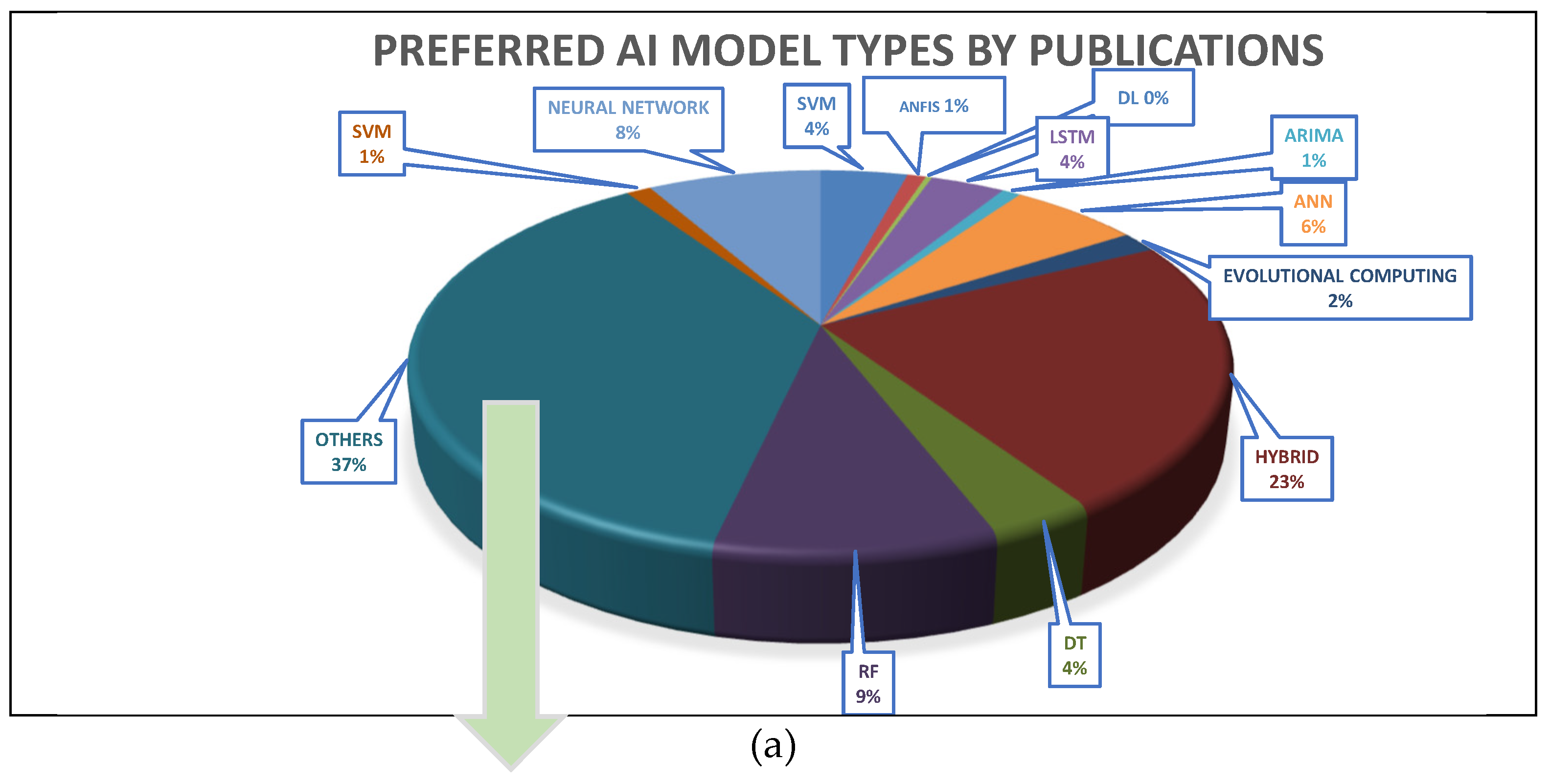
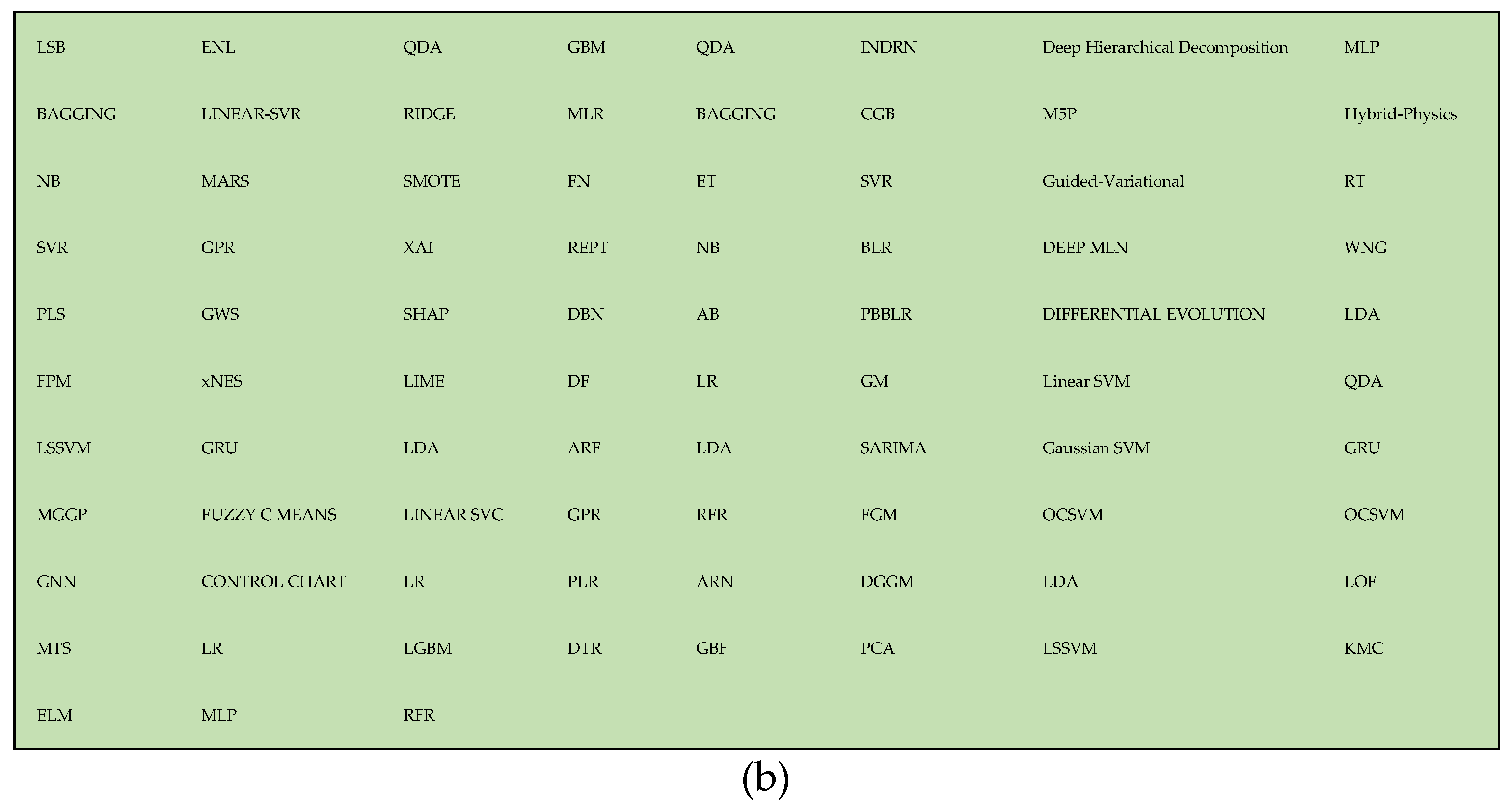
The analysis of predictive analytics research publications from 2021 to 2023 focuses heavily on several areas of the O&G sector. Crude oils (7), oil (5), reservoirs (16), pipelines (16), drilling (5), wells (20), transformers (10), gas (10), and lithology (2) all appear as recurring topics in various research. The frequency of these terms demonstrates the industry's strong interest in using predictive analytics to optimize operations and decision-making in various sectors, including reservoir management, drilling procedures, pipeline integrity, and transformer health. This trend represents a deliberate effort in the O&G industry to use sophisticated analytics for greater efficiency, risk management, and overall operational excellence. Figure 5 is the graphical summary of the types of O&G sectors in research articles.

Figure 5. Types of O&G Sectors in Research Articles from 2021 to 2023.

Figure 5. Types of O&G Sectors in Research Articles from 2021 to 2023.
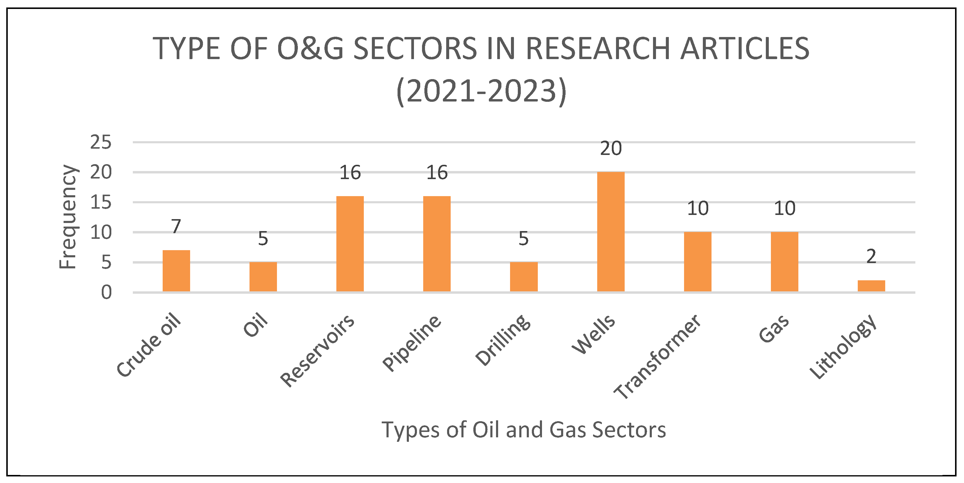
Several performance measures have been utilized in O&G sector research, demonstrating diverse assessment criteria for predictive analytics models (see Figure 6). The performance metrics help understand the models' performance since they might show many model characteristics. Figure 6 (a), which shows the various performance measures used in the research, demonstrates that accuracy (49) was the most preferred for calculating the correctly predicted value versus the actual. This performance measure is appropriate for categorical data types and classification predictive analysis because it is simple to grasp and indicates whether all classes are balanced. However, utilizing accuracy for unbalanced classes has limitations since it can be deceptive; alternative measures like precision, recall, F1-score, or area under the AUC may be more helpful. Aside from that, the researchers' second chosen performance indicator in their research is R2 (41). This performance indicator is commonly employed in regression analysis and numerical data since it measures the relationship between the independent and dependent variables.

Figure 6. Preferred Performance Metrics by Researcher: (a) Combination of Performance Metrics used in publications. (b) Display all the other performance metrics beyond the most common ones.

Figure 6. Preferred Performance Metrics by Researcher: (a) Combination of Performance Metrics used in publications. (b) Display all the other performance metrics beyond the most common ones.
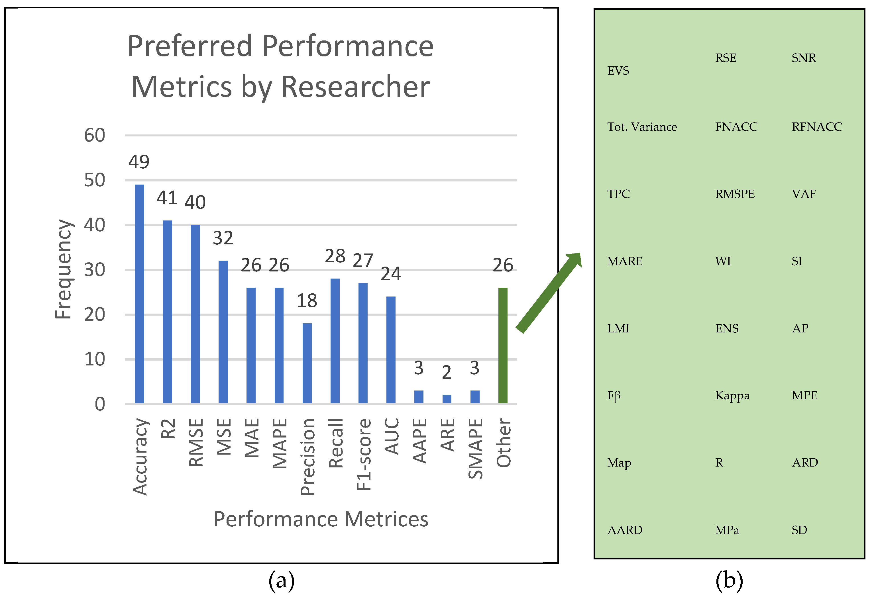
Furthermore, R2 is simple to read because it ranges from 0 to 1, with closer results to 1 indicating perfect variability between independent and dependent variables. However, there is a disadvantage to using only R2 to demonstrate how effectively the model reacts. One of the disadvantages is that it is vulnerable to outliers; even a single outlier might alter the results. Figure 6 (b) is an expansion of "others" that depicts the additional performance indicators used in the previous studies.

4. Future Research Direction

As predictive analytics in the O&G industry continues to evolve, several avenues for future research and development emerge. Firstly, exploring the integration of advanced deep learning techniques, such as RNN and LSTM networks, could enhance the temporal predictive capabilities of existing models. These architectures are adept at capturing sequential dependencies and time-series patterns, which could prove invaluable for forecasting dynamic aspects like O&G production rates or pipeline conditions. Secondly, investigating explainability and interpretability in complex models, such as ensemble techniques and deep learning networks, remains a meaningful direction. Developing methods to elucidate the decision-making processes of these models can enhance the trust and acceptance of predictive analytics in decision support systems within the O&G domain.

Furthermore, there is potential for extending research into the optimization of hybrid models, focusing on refining parameter-tuning strategies and evaluating the robustness of these approaches across diverse datasets and scenarios. For instance, understanding how QPSO or FDGGM parameters impact model performance could lead to more effective and efficient hybrid predictive systems. Additionally, exploring predictive analytics for emerging challenges in the industry, such as sustainability, environmental impact, and safety, could open new avenues for research. Predicting the environmental consequences of O&G activities or developing models for proactive safety monitoring could contribute significantly to the industry's responsible and sustainable practices.

Finally, comprehensive benchmarking studies are needed to compare the performance of various predictive models under many circumstances and datasets. This could facilitate the identification of the most suitable models for specific applications within the O&G sector, providing practitioners with insightful information for making decisions. In conclusion, future research in predictive analytics for the O&G industry should delve into advanced deep learning architectures, enhance model interpretability, optimize hybrid approaches, address emerging challenges, and conduct systematic benchmarking studies to advance the state-of-the-art in this critical domain.

5. Conclusions

The present study was initiated to provide a thorough overview of the utilization of ML models in simulating predictive analytics within the O&G sectors. From 2021 to 2023, the research study collected data from respectable journals indexed in Web of Science, Science Direct, Scopus, and IEEE. The analysis revealed that seven iterations of ML models had been employed in predictive analytics modelling for the O&G industry. The survey identified key components within existing predictive analytics models for O&G, encompassing model types, temporal aspects of data, field, and name of the data, dataset types, predictive analytics methodologies (classification, clustering, or prediction), input and output parameters of the model, performance metrics, optimal models, and associated advantages and limitations. Rigorous scientific assessments and evaluations were conducted on the surveyed studies, leading to detailed discussions on numerous findings. The study also highlights various potential future research directions based on the current state of literature, providing insightful information to interested professionals in this sector.

Author Contributions

P.A.; writing—original draft preparation, visualization; M.Y.; review and editing, supervision; M.T.; funding acquisition. All authors have read and agreed to the published version of the manuscript.

Funding

This research was funded by Petronas Research Sdn. Bhd. (PRSB), grant number 20220801012.

Institutional Review Board Statement

Not applicable.

Informed Consent Statement

Not applicable.

Data Availability Statement

The study did not report any data.

Conflicts of Interest

The authors declare no conflicts of interest.

Abbreviations

Table 11. A list of abbreviations and their descriptions used in this study.

Abbreviations	Definition	Abbreviations	Definition
RF	Random Forest	DNN	Deep Neural Network
GAM	Generalized Additive Model	MELM	Multivariate Empirical Mode Decomposition
NN	Neural Network	ANFIS	Adaptive Neuro-Fuzzy Inference System
SVR-GA	Support Vector Regression with Genetic Algorithm	SOM	Self-Organizing Map
SVR-PSO	Support Vector Regression with Particle Swarm Optimization	ANN	Artificial Neural Network
SVR-FFA	Support Vector Regression with Firefly Algorithm	MRGC	Maximum Relevant Gain Clustering
GB	Gradient Boosting	CatBoost	Categorical Boosting
LSSVM-CSA	Least Squares Support Vector Machine with Cuckoo Search Algorithm	MLR	Multiple Linear Regression
AHC	Agglomerative Hierarchical Clustering	SVM	Support Vector Machine
XGBoost	Extreme Gradient Boosting	FN	Fuzzy Network
GPR	Gaussian Process Regression	LDA	Linear Discriminant Analysis
LWQPSO-ANN	Linearly Weighted Quantum Particle Swarm Optimization with Artificial Neural Network	LSSVM	Least Squares Support Vector Machine
PCA	Principal Component Analysis	DL	Deep Learning
MLP-ANN	Multilayer Perceptron with Artificial Neural Network	MLSTM	Multilayer Long Short-Term Memory
MLP-PSO	Multilayer Perceptron with Particle Swarm Optimization	GRU	Gated Recurrent Unit
DT	Decision Tree	AdaBoost	Adaptive Boosting
LSTM	Long Short-Term Memory	LSTM-AE-IF	Long Short-Term Memory Autoencoder with Isolation Forest
KNN	k-Nearest Neighbors	DNN	Deep Neural Network
NB	Naive Bayes	CNN	Convolutional Neural Network
GP	Genetic Programming	O&G	Oil and Gas
ELM	Extreme Learning Machine	AI	Artificial Intelligence
DF	Deep Forest	MSE	Mean Squared Error
QDA	Quadratic Discriminant Analysis	MAPE	Mean Absolute Percentage Error
ML	Machine Learning	AAPE	Arithmetic Average Percentage Error
DGA	Dissolved Gas Analysis	SMAPE	Symmetric Mean Absolute Percentage Error
RMSE	Root Mean Squared Error	RSE	Relative Squared Error
MAE	Mean Absolute Error	RFR	Random Forest Regression
AUC	Area Under the Curve	FNACC	Faulty-normal accuracy
ARE	Absolute Relative Error	TPC	Total Percent of Correct
EVS	Explained Variance Score	VAF	Variance Accounted For
DTR	Decision Tree Regression	WI	Weighted Index
PLR	Polynomial Linear Regression	LMI	Linear Mean Index
SNR	Signal-to-Noise Ratio	AP	Average Precision
RFNACC	Real Faulty-Normal Accuracy	MAP	Mean Average Percentage
RMSPE	Root Mean Square Percentage Error	ARD	Absolute Relative Difference
MARE	Mean Absolute Relative Error	Mpa	Megapascal
SI	Severity Index	P-JUS-CKGL	Pressure downstream of gas lift choke
ENS	Energy Normalized Score	P-CKGL	Pressure downstream of gas lift choke CKGL
MPE	Mean Percentage Error	QGL	Gas lift flow rate
R	Correlation of Coefficient	T-PDG	Temperature at the permanent downhole gauge sensor
AARD	Average Absolute Relative Deviation	T-PCK	Temperature downstream of the production choke
P-PDG	Pressure at permanent downhole gauge PDG	LSB	Least Square Boosting
P-TPT	Pressure at temperature/pressure transducer TPT	PLS	Partial Least Squares
T-TPT	Temperature at TPT	FPM	Feature Projection Model
P-MON-CKP	Pressure upstream of production choke CKP	FP-DNN	Feature Projection-Deep Neural Network
T-JUS-CKP	Pressure downstream of CKP	GNN	Graph Neural Network
T-JUS-CKGL	Temperature downstream of CKGL	MLP	Multilayer perceptron
FP-PLS	Feature Projection-PLS	Bi-LSTM	Bidirectional Long Short-Term
MGGP	Multi-Gene Genetic Programming	SHAP	Shapley Additive Explanation
xNES	Exponential natural evolution strategies	LR	Logistic Regression
RNN	Recurrent Neural Network	LOF	Local Outlier Factor
LGBM	Light Gradient Boosting Machine	ICA	Imperialist Competitive Algorithm
SMOTE	Synthetic Minority Oversampling Technique	SFLA	Shuffled Frog-Leaping Algorithm
LIME	Local Interpretable Model-Agnostic Explanations	SA	Simulated Annealing
XAI	Explainable Artificial Intelligence	PBBLR	Physics-Based Bayesian Linear Regression
GSK	Gaining-sharing knowledge-based algorithm	ARIMA	Autoregressive Integrated Moving Average
BayesOpt-XGBoost	Bayesian optimization XGBoost	GM	Generalized Method of Moments
FA	Firefly Algorithm	PSO-FDGGM	PSO-based data grouping grey model with a fractional order accumulation
COA	Cuckoo Optimization Algorithm	PSOGM	PSO for Grey Model
GWO	Grey Wolf Optimizer	LSSVM	Least-Square Support Vector Machine
HAS	Harmony Search	GA	Genetic Algorithm
BLR	Bayesian Linear Regression	OCSVM	One-Class Support Vector Machine
SARIMA	Seasonal Autoregressive Integrated Moving Average	BAE	Basic Autoencoder
GM	Grey model	CAE	Convolutional Autoencoder
FGM	Fractional grey model	AE	Autoencoder
DGGM	Data Grouping-Based Grey Modelling Method	VAE	Variational Autoencoders
GPR	Gaussian Process Regression	MARS	Multivariate Adaptive Regression Splines

References

J. Liang et al., “Activation of mixed sawdust and spirulina with or without a pre-carbonization step: Probing roles of volatile-char interaction on evolution of pyrolytic products,” Fuel Process. Technol., vol. 250, no. July, p. 107926, 2023. [CrossRef]
L. Xu, Y. Wang, L. Mo, Y. Tang, F. Wang, and C. Li, “The research progress and prospect of data mining methods on corrosion prediction of oil and gas pipelines,” Eng. Fail. Anal., vol. 144, no. June 2022, p. 106951, 2023. [CrossRef]
R. Sharma and B. Villányi, “Evaluation of corporate requirements for smart manufacturing systems using predictive analytics,” Internet of Things (Netherlands), vol. 19. Elsevier B.V., Aug. 01, 2022. [CrossRef]
K. Henrys, “Role of Predictive Analytics in Business,” SSRN Electron. J., no. March, 2021. [CrossRef]
S. Tewari, U. D. Dwivedi, and S. Biswas, “A novel application of ensemble methods with data resampling techniques for drill bit selection in the oil and gas industry,” Energies, vol. 14, no. 2, 2021. [CrossRef]
I. Allouche, Q. Zheng, N. Yoosef-Ghodsi, M. Fowler, Y. Li, and S. Adeeb, “Enhanced predictive method for pipeline strain demand subject to permanent ground displacements with internal pressure & temperature: a finite difference approach,” J. Infrastruct. Intell. Resil., vol. 2, no. 4, p. 100030, 2023. [CrossRef]
B. G. Carvalho, R. E. Vaz Vargas, R. M. Salgado, C. J. Munaro, and F. M. Varejao, “Flow Instability Detection in Offshore Oil Wells with Multivariate Time Series Machine Learning Classifiers,” IEEE Int. Symp. Ind. Electron., vol. 2021-June, 2021. [CrossRef]
Nzubechukwu Chukwudum Ohalete, Adebayo Olusegun Aderibigbe, Emmanuel Chigozie Ani, Peter Efosa Ohenhen, and Abiodun Akinoso, “Advancements in predictive maintenance in the oil and gas industry: A review of AI and data science applications,” World J. Adv. Res. Rev., vol. 20, no. 3, pp. 167–181, 2023. [CrossRef]
Z. Tariq et al., A systematic review of data science and machine learning applications to the oil and gas industry, vol. 11, no. 12. Springer International Publishing, 2021.
X. Yu, J. Wang, Q.-Q. Hong, R. Teku, S.-H. Wang, and Y.-D. Zhang, “Transfer learning for medical images analyses: A survey,” Neurocomputing, vol. 489, pp. 230–254, 2022. [CrossRef]
B. D. Barkana, Y. Ozkan, and J. A. Badara, “Analysis of working memory from EEG signals under different emotional states,” Biomed. Signal Process. Control, vol. 71, p. 103249, 2022. [CrossRef]
W. Chen, H. Huang, J. Huang, K. Wang, H. Qin, and K. K. L. Wong, “Deep learning-based medical image segmentation of the aorta using XR-MSF-U-Net,” Comput. Methods Programs Biomed., vol. 225, p. 107073, 2022. [CrossRef]
C. Huang, B. Gu, Y. Chen, X. Tan, and L. Feng, “Energy return on energy, carbon, and water investment in oil and gas resource extraction: Methods and applications to the Daqing and Shengli oilfields,” Energy Policy, vol. 134, p. 110979, 2019. [CrossRef]
S. Hazboun and H. Boudet, “Chapter 8 - A ‘thin green line’ of resistance? Assessing public views on oil, natural gas, and coal export in the Pacific Northwest region of the United States and Canada,” in Public Responses to Fossil Fuel Export, H. Boudet and S. Hazboun, Eds. Elsevier, 2022, pp. 121–139.
A. Champeecharoensuk, S. Dhakal, N. Chollacoop, and A. Phdungsilp, “Greenhouse gas emissions trends and drivers insights from the domestic aviation in Thailand,” Heliyon, vol. 10, no. 2, p. e24206, 2024. [CrossRef]
P. Centobelli, R. Cerchione, P. Del Vecchio, E. Oropallo, and G. Secundo, “Blockchain technology for bridging trust, traceability and transparency in circular supply chain,” Inf. Manag., vol. 59, no. 7, p. 103508, 2022. [CrossRef]
H. Majed, S. Al-Janabi, and S. Mahmood, “Data Science for Genomics (GSK- XGBoost) for Prediction Six Types of Gas Based on Intelligent Analytics,” 2022, pp. 28–34. [CrossRef]
A. Waterworth and M. J. Bradshaw, “Unconventional trade-offs? National oil companies, foreign investment and oil and gas development in Argentina and Brazil,” Energy Policy, vol. 122, pp. 7–16, 2018. [CrossRef]
M. A. Marins et al., “Fault detection and classification in oil wells and production/service lines using random forest,” J. Pet. Sci. Eng., vol. 197, no. August 2020, p. 107879, 2021. [CrossRef]
D. K. Dhaked, S. Dadhich, and D. Birla, “Power output forecasting of solar photovoltaic plant using LSTM,” Green Energy Intell. Transp., vol. 2, no. 5, p. 100113, 2023. [CrossRef]
R. Yan, S. Wang, and C. Peng, “An Artificial Intelligence Model Considering Data Imbalance for Ship Selection in Port State Control Based on Detention Probabilities,” J. Comput. Sci., vol. 48, no. July 2020, p. 101257, 2021. [CrossRef]
O. E. Agwu, E. E. Okoro, and S. E. Sanni, “Modelling oil and gas flow rate through chokes: A critical review of extant models,” J. Pet. Sci. Eng., vol. 208, p. 109775, 2022. [CrossRef]
K. Nandhini and G. Tamilpavai, “Hybrid CNN-LSTM and modified wild horse herd Model-based prediction of genome sequences for genetic disorders,” Biomed. Signal Process. Control, vol. 78, p. 103840, 2022. [CrossRef]
S. Balaji and S. Karthik, “Deep Learning Based Energy Consumption Prediction on Internet of Things Environment,” Intell. Autom. SOFT Comput., vol. 37, no. 1, pp. 727–743, 2023. [CrossRef]
H. Yang et al., “Optimization of tight gas reservoir fracturing parameters via gradient boosting regression modeling,” Heliyon, vol. 10, no. 5, p. e27015, 2024. [CrossRef]
M. de los Ángeles Sánchez Morales and F. I. Soler Anguiano, “Data science - time series analysis of oil & gas production in mexican fields,” Procedia Comput. Sci., vol. 200, pp. 21–30, 2022. [CrossRef]
Y. Tan, A. A. Al-Huqail, Q. S. Chen, H. S. Majdi, J. S. Algethami, and H. E. Ali, “Analysis of groundwater pollution in a petroleum refinery energy contributed in rock mechanics through ANFIS-AHP,” Int. J. ENERGY Res., vol. 46, no. 15, pp. 20928–20938, 2022. [CrossRef]
M. Wu, G. Wang, and H. Liu, “Research on Transformer Fault Diagnosis Based on SMOTE and Random Forest,” Proc. - 2022 4th Int. Conf. Electr. Eng. Control Technol. CEECT 2022, pp. 359–363, 2022. [CrossRef]
Q. Dashti et al., “Data Analytics into Hydraulic Modelling for Better Understanding of Well/Surface Network Limits, Proactively Identify Challenges and, Provide Solutions for Improved System Performance in the Greater Burgan Field,” 2021. [CrossRef]
X. Wang, M. Daryapour, A. Shahrabadi, S. Pirasteh, and F. Razavirad, “Artificial neural networks in predicting of the gas molecular diffusion coefficient,” Chem. Eng. Res. Des., vol. 200, pp. 407–418, 2023. [CrossRef]
R. Kamarudin et al., “Influence of oxyhydrogen gas retrofit into two-stroke engine on emissions and exhaust gas temperature variations,” Heliyon, vol. 10, no. 5, p. e26597, 2024. [CrossRef]
R. Raghuraman and A. Darvishi, “Detecting Transformer Fault Types from Dissolved Gas Analysis Data Using Machine Learning Techniques,” 2022. [CrossRef]
T. Mukherjee, T. Burgett, T. Ghanchi, C. Donegan, and T. Ward, “Predicting Gas Production Using Machine Learning Methods: A Case Study,” 2019, pp. 2248–2252. [CrossRef]
N. Dixit, P. McColgan, and K. Kusler, “Machine Learning-Based Probabilistic Lithofacies Prediction from Conventional Well Logs: A Case from the Umiat Oil Field of Alaska,” Energies, vol. 13, no. 18, p. 4862, Sep. 2020. [CrossRef]
H. Aldosari, R. Elfouly, and R. Ammar, “Evaluation of Machine Learning-Based Regression Techniques for Prediction of Oil and Gas Pipelines Defect,” in 2020 International Conference on Computational Science and Computational Intelligence (CSCI), Dec. 2020, pp. 1452–1456. [CrossRef]
H. H. Elmousalami and M. Elaskary, “Drilling stuck pipe classification and mitigation in the Gulf of Suez oil fields using artificial intelligence,” J. Pet. Explor. Prod. Technol., vol. 10, no. 5, pp. 2055–2068, Jun. 2020. [CrossRef]
I. B. M. Taha and D.-E. A. Mansour, “Novel Power Transformer Fault Diagnosis Using Optimized Machine LearningMethods,” Intell. Autom. SOFT Comput., vol. 28, no. 3, pp. 739–752, 2021. [CrossRef]
Tiyasha, T. M. Tung, and Z. M. Yaseen, “A survey on river water quality modelling using artificial intelligence models: 2000–2020,” J. Hydrol., vol. 585, p. 124670, 2020. [CrossRef]
S. Agatonovic-Kustrin and R. Beresford, “Basic concepts of artificial neural network (ANN) modeling and its application in pharmaceutical research,” J. Pharm. Biomed. Anal., vol. 22, no. 5, pp. 717–727, 2000. [CrossRef]
H. Tao et al., “Groundwater level prediction using machine learning models: A comprehensive review,” Neurocomputing, vol. 489, pp. 271–308, 2022. [CrossRef]
S. Kalam, U. Yousuf, S. A. Abu-Khamsin, U. Bin Waheed, and R. A. Khan, “An ANN model to predict oil recovery from a 5-spot waterflood of a heterogeneous reservoir,” J. Pet. Sci. Eng., vol. 210, p. 110012, Mar. 2022. [CrossRef]
E. Eckert, Z. Bělohlav, T. Vaněk, P. Zámostný, and T. Herink, “ANN modelling of pyrolysis utilising the characterisation of atmospheric gas oil based on incomplete data,” Chem. Eng. Sci., vol. 62, no. 18, pp. 5021–5025, 2007. [CrossRef]
G. Qin, A. Xia, H. Lu, Y. Wang, R. Li, and C. Wang, “A hybrid machine learning model for predicting crater width formed by explosions of natural gas pipelines,” J. Loss Prev. Process Ind., vol. 82, p. 104994, Apr. 2023. [CrossRef]
Q. Wang et al., “Evolution of corrosion prediction models for oil and gas pipelines: From empirical-driven to data-driven,” Eng. Fail. Anal., vol. 146, p. 107097, 2023. [CrossRef]
N. A. Sami and D. S. Ibrahim, “Forecasting multiphase flowing bottom-hole pressure of vertical oil wells using three machine learning techniques,” Pet. Res., vol. 6, no. 4, pp. 417–422, 2021. [CrossRef]
H. Qayyum Chohan, I. Ahmad, N. Mohammad, D. Manca, and H. Caliskan, “An integrated approach of artificial neural networks and polynomial chaos expansion for prediction and analysis of yield and environmental impact of oil shale retorting process under uncertainty,” Fuel, vol. 329, p. 125351, Dec. 2022. [CrossRef]
G. de A. Carvalho, P. J. Minnett, N. F. F. Ebecken, and L. Landau, “Machine-Learning Classification of SAR Remotely-Sensed Sea-Surface Petroleum Signatures—Part 1: Training and Testing Cross Validation,” Remote Sens., vol. 14, no. 13, 2022. [CrossRef]
X. Li, W. Han, W. Shao, L. Chen, and D. Zhao, “Data-Driven Predictive Model for Mixed Oil Length Prediction in Long-Distance Transportation Pipeline,” in 2021 IEEE 10th Data Driven Control and Learning Systems Conference (DDCLS), May 2021, pp. 1486–1491. [CrossRef]
J. H. Mendoza, R. Tariq, L. F. S. Espinosa, F. Anguebes, A. Bassam, and IEEE, “Soft Computing Tools for Multiobjective Optimization of Offshore Crude Oil and Gas Separation Plant for the Best Operational Condition,” 2021 18TH INTERNATIONAL CONFERENCE ON ELECTRICAL ENGINEERING, COMPUTING SCIENCE AND AUTOMATIC CONTROL (CCE 2021), no. 18th International Conference on Electrical Engineering, Computing Science and Automatic Control (CCE). 2021. [CrossRef]
A. Sakhaei, S. M. Zamir, E. R. Rene, M. C. Veiga, and C. Kennes, “Neural network-based performance assessment of one- and two-liquid phase biotrickling filters for the removal of a waste-gas mixture containing methanol, α-pinene, and hydrogen sulfide,” Environ. Res., vol. 237, p. 116978, 2023. [CrossRef]
M. Hasanzadeh and M. Madani, “Deterministic tools to predict gas assisted gravity drainage recovery factor,” Energy Geosci., p. 100267, 2023. [CrossRef]
X.-Q. Zhang, Q.-L. Cheng, W. Sun, Y. Zhao, and Z.-M. Li, “Research on a TOPSIS energy efficiency evaluation system for crude oil gathering and transportation systems based on a GA-BP neural network,” Pet. Sci., 2023. [CrossRef]
A. Ismail, H. F. Ewida, S. Nazeri, M. G. Al-Ibiary, and A. Zollo, “Gas channels and chimneys prediction using artificial neural networks and multi-seismic attributes, offshore West Nile Delta, Egypt,” J. Pet. Sci. Eng., vol. 208, 2022. [CrossRef]
L. Goliatt, C. M. Saporetti, L. C. Oliveira, and E. Pereira, “Performance of evolutionary optimized machine learning for modeling total organic carbon in core samples of shale gas fields,” Petroleum, 2023. [CrossRef]
M. N. Amar, A. J. Ghahfarokhi, C. S. W. Ng, and N. Zeraibi, “Optimization of WAG in real geological field using rigorous soft computing techniques and nature-inspired algorithms,” J. Pet. Sci. Eng., vol. 206, 2021. [CrossRef]
W. Mao et al., “Power transformers fault diagnosis using graph neural networks based on dissolved gas data,” in Journal of Physics: Conference Series, 2022, vol. 2387, no. 1. [CrossRef]
I. Ghosh, T. D. Chaudhuri, E. Alfaro-Cortés, M. Gámez, and N. García, “A hybrid approach to forecasting futures prices with simultaneous consideration of optimality in ensemble feature selection and advanced artificial intelligence,” Technol. Forecast. Soc. Change, vol. 181, Aug. 2022. [CrossRef]
B. Wang, Y. Guo, D. Wang, Y. Zhang, R. He, and J. Chen, “Prediction model of natural gas pipeline crack evolution based on optimized DCNN-LSTM,” Mech. Syst. Signal Process., vol. 181, Dec. 2022. [CrossRef]
G. Antariksa, R. Muammar, A. Nugraha, and J. Lee, “Deep sequence model-based approach to well log data imputation and petrophysical analysis: A case study on the West Natuna Basin, Indonesia,” J. Appl. Geophys., vol. 218, 2023. [CrossRef]
R. de O. Werneck et al., “Data-driven deep-learning forecasting for oil production and pressure,” J. Pet. Sci. Eng., vol. 210, p. 109937, Mar. 2022. [CrossRef]
S. Das, A. Paramane, S. Chatterjee, and U. M. Rao, “Accurate Identification of Transformer Faults From Dissolved Gas Data Using Recursive Feature Elimination Method,” IEEE Trans. Dielectr. Electr. Insul., vol. 30, no. 1, pp. 466–473, 2023. [CrossRef]
H. S. Barjouei et al., “Prediction performance advantages of deep machine learning algorithms for two-phase flow rates through wellhead chokes,” J. Pet. Explor. Prod. Technol., vol. 11, no. 3, pp. 1233–1261, Mar. 2021. [CrossRef]
V. Martinez and A. Rocha, “The Golem: A General Data-Driven Model for Oil & Gas Forecasting Based on Recurrent Neural Networks,” IEEE Access, vol. 11, pp. 41105 – 41132, 2023. [CrossRef]
Z. B. Wang et al., “Optimized faster R-CNN for oil wells detection from high-resolution remote sensing images,” Int. J. Remote Sens., vol. 44, no. 22, pp. 6897–6928, 2023. [CrossRef]
A. Hiassat, A. Diabat, and I. Rahwan, “A genetic algorithm approach for location-inventory-routing problem with perishable products,” J. Manuf. Syst., vol. 42, pp. 93–103, 2017. [CrossRef]
V. Sharma, Ü. Cali, B. Sardana, M. Kuzlu, D. Banga, and M. Pipattanasomporn, “Data-driven short-term natural gas demand forecasting with machine learning techniques,” J. Pet. Sci. Eng., vol. 206, Nov. 2021. [CrossRef]
H. C. Phan and H. T. Duong, “Predicting burst pressure of defected pipeline with Principal Component Analysis and adaptive Neuro Fuzzy Inference System,” Int. J. Press. Vessel. Pip., vol. 189, 2021. [CrossRef]
A. O. De Salvo Castro, M. De Jesus Rocha Santos, F. R. Leta, C. B. C. Lima, and G. B. A. Lima, “Unsupervised Methods to Classify Real Data from Offshore Wells,” Am. J. Oper. Res., vol. 11, no. 05, pp. 227–241, 2021. [CrossRef]
H. Hamedi, S. Zendehboudi, N. Rezaei, N. M. C. Saady, and B. Zhang, “Modeling and optimization of oil adsorption capacity on functionalized magnetic nanoparticles using machine learning approach,” J. Mol. Liq., vol. 392, p. 123378, Dec. 2023. [CrossRef]
B. Ma, J. Shuai, D. Liu, and K. Xu, “Assessment on failure pressure of high strength pipeline with corrosion defects,” Eng. Fail. Anal., vol. 32, pp. 209–219, 2013.
Y. Shuai, J. Shuai, and K. Xu, “Probabilistic analysis of corroded pipelines based on a new failure pressure model,” Eng. Fail. Anal., vol. 81, pp. 216–233, 2017.
H. C. Phan, A. S. Dhar, and B. C. Mondal, “Revisiting burst pressure models for corroded pipelines,” Can. J. Civ. Eng., vol. 44, no. 7, pp. 485–494, 2017.
J. L. F. Freire, R. D. Vieira, J. T. P. Castro, and A. C. Benjamin, “Part 3: Burst tests of pipeline with extensive longitudinal metal loss,” Exp. Tech., vol. 30, pp. 60–65, 2006.
D. S. Cronin, “Assessment of corrosion defects in pipelines,” 2000.
A. Ghasemieh, A. Lloyed, P. Bahrami, P. Vajar, and R. Kashef, “A novel machine learning model with Stacking Ensemble Learner for predicting emergency readmission of heart-disease patients,” Decis. Anal. J., vol. 7, p. 100242, 2023. [CrossRef]
J. R. V. Jeny, N. S. Reddy, P. Aishwarya, and Samreen, “A Classification Approach for Heart Disease Diagnosis using Machine Learning,” Proc. IEEE Int. Conf. Signal Process. Control, vol. 2021-Octob, pp. 456–459, 2021. [CrossRef]
R. K. Mazumder, A. M. Salman, and Y. Li, “Failure risk analysis of pipelines using data-driven machine learning algorithms,” Struct. Saf., vol. 89, p. 102047, Mar. 2021. [CrossRef]
S. Liu, Y. Zhao, and Z. Wang, “Artificial Intelligence Method for Shear Wave Travel Time Prediction considering Reservoir Geological Continuity,” Math. Probl. Eng., vol. 2021, 2021. [CrossRef]
S. Saroja, S. Haseena, and R. Madavan, “Dissolved Gas Analysis of Transformer: An Approach Based on ML and MCDM,” IEEE Trans. Dielectr. Electr. Insul., Oct. 2023. [CrossRef]
R. A. Raj, D. Sarathkumar, S. K. Venkatachary, and L. J. B. Andrews, “Classification and Prediction of Incipient Faults in Transformer Oil by Supervised Machine Learning using Decision Tree,” 2023. [CrossRef]
N. Aslam et al., “Anomaly Detection Using Explainable Random Forest for the Prediction of Undesirable Events in Oil Wells,” Appl. Comput. Intell. Soft Comput., vol. 2022, 2022. [CrossRef]
E. M. Turan and J. Jaschke, “Classification of undesirable events in oil well operation,” Proc. 2021 23rd Int. Conf. Process Control. PC 2021, pp. 157–162, 2021. [CrossRef]
F. Gatta, F. Giampaolo, D. Chiaro, and F. Piccialli, “Predictive maintenance for offshore oil wells by means of deep learning features extraction,” Expert Syst., no. August, pp. 1–13, 2022. [CrossRef]
C. Brønstad, S. L. Netto, and A. L. L. Ramos, “Data-driven Detection and Identification of Undesirable Events in Subsea Oil Wells,” SENSORDEVICES 2021 Twelfth Int. Conf. Sens. Device Technol. Appl., no. c, pp. 1–6, 2021.
S. Ben Jabeur, R. Khalfaoui, and W. Ben Arfi, “The effect of green energy, global environmental indexes, and stock markets in predicting oil price crashes: Evidence from explainable machine learning,” J. Environ. Manage., vol. 298, p. 113511, Nov. 2021. [CrossRef]
H. K. Hassan Baabbad, E. Artun, and B. Kulga, “Understanding the Controlling Factors for CO2 Sequestration in Depleted Shale Reservoirs Using Data Analytics and Machine Learning,” Jun. 2022. [CrossRef]
A. Alsaihati, S. Elkatatny, A. A. Mahmoud, and A. Abdulraheem, “Use of Machine Learning and Data Analytics to Detect Downhole Abnormalities while Drilling Horizontal Wells, with Real Case Study,” J. Energy Resour. Technol. Trans. ASME, vol. 143, no. 4, 2021. [CrossRef]
A. Kumar and H. Hassanzadeh, “A qualitative study of the impact of random shale barriers on SAGD performance using data analytics and machine learning,” J. Pet. Sci. Eng., vol. 205, 2021. [CrossRef]
H. Ma, H. Wang, M. Geng, Y. Ai, W. Zhang, and W. Zheng, “A new hybrid approach model for predicting burst pressure of corroded pipelines of gas and oil,” Eng. Fail. Anal., vol. 149, p. 107248, Jul. 2023. [CrossRef]
G. Canonaco et al., “A Machine-Learning Approach for the Prediction of Internal Corrosion in Pipeline Infrastructures,” in 2021 IEEE International Instrumentation and Measurement Technology Conference (I2MTC), May 2021, vol. 2021-May, pp. 1–6. [CrossRef]
J. Fang, X. Cheng, H. Gai, S. Lin, and H. Lou, “Development of machine learning algorithms for predicting internal corrosion of crude oil and natural gas pipelines,” Comput. Chem. Eng., vol. 177, p. 108358, 2023. [CrossRef]
Q. Lv et al., “Modelling minimum miscibility pressure of CO2-crude oil systems using deep learning, tree-based, and thermodynamic models: Application to CO2 sequestration and enhanced oil recovery,” Sep. Purif. Technol., vol. 310, p. 123086, 2023. [CrossRef]
X. Zhu et al., “An automatic identification method of imbalanced lithology based on Deep Forest and K-means SMOTE,” Geoenergy Sci. Eng., vol. 224, no. May 2022, p. 211595, 2023. [CrossRef]
H. Majed, S. Al-Janabi, and S. Mahmood, “Data Science for Genomics (GSK- XGBoost) for Prediction Six Types of Gas Based on Intelligent Analytics,” in 2022 22nd International Conference on Computational Science and Its Applications (ICCSA), 2022, pp. 28–34. [CrossRef]
P. Chanchotisatien and C. Vong, “Feature engineering and feature selection for fault type classification from dissolved gas values in transformer oil,” in ICSEC 2021 - 25th International Computer Science and Engineering Conference, 2021, pp. 75–80. [CrossRef]
M. de J. R. Santos et al., “Statistical analysis of offshore production sensors for failure detection applications / Análise estatística dos sensores de produção offshore para aplicações de detecção de falhas,” Brazilian J. Dev., vol. 7, no. 8, pp. 85880–85898, 2021. [CrossRef]
M. Ali et al., “Reservoir characterization through comprehensive modeling of elastic logs prediction in heterogeneous rocks using unsupervised clustering and class-based ensemble machine learning,” Appl. Soft Comput., vol. 148, 2023. [CrossRef]
C. Ashayeri and B. Jha, “Evaluation of transfer learning in data-driven methods in the assessment of unconventional resources,” J. Pet. Sci. Eng., vol. 207, 2021. [CrossRef]
P. Vuttipittayamongkol, A. Tung, and E. Elyan, “A Data-Driven Decision Support Tool for Offshore Oil and Gas Decommissioning,” IEEE Access, vol. 9, pp. 137063–137082, 2021. [CrossRef]
T. Song et al., “A novel well-logging data generation model integrated with random forests and adaptive domain clustering algorithms,” Geoenergy Sci. Eng., vol. 231, 2023. [CrossRef]
B. Awuku, Y. Huang, and N. Yodo, “Predicting Natural Gas Pipeline Failures Caused by Natural Forces: An Artificial Intelligence Classification Approach,” Appl. Sci., vol. 13, no. 7, 2023. [CrossRef]
W. J. Al-Mudhafar, M. A. Abbas, and D. A. Wood, “Performance evaluation of boosting machine learning algorithms for lithofacies classification in heterogeneous carbonate reservoirs,” Mar. Pet. Geol., vol. 145, 2022. [CrossRef]
H. Wen, L. Liu, J. Zhang, J. Hu, and X. Huang, “A hybrid machine learning model for landslide-oriented risk assessment of long-distance pipelines,” J. Environ. Manage., vol. 342, 2023. [CrossRef]
D. A. Otchere, T. O. A. Ganat, V. Nta, E. T. Brantson, and T. Sharma, “Data analytics and Bayesian Optimised Extreme Gradient Boosting approach to estimate cut-offs from wireline logs for net reservoir and pay classification,” Appl. Soft Comput., vol. 120, 2022. [CrossRef]
H. Gamal, S. Elkatatny, A. Alsaihati, and A. Abdulraheem, “Intelligent Prediction for Rock Porosity while Drilling Complex Lithology in Real Time,” Comput. Intell. Neurosci., vol. 2021, 2021. [CrossRef]
M. F. H. Ismail, Z. May, V. S. Asirvadam, and N. A. Nayan, “Machine-Learning-Based Classification for Pipeline Corrosion with Monte Carlo Probabilistic Analysis,” Energies, vol. 16, no. 8, 2023. [CrossRef]
R. A. Prasojo et al., “Precise transformer fault diagnosis via random forest model enhanced by synthetic minority over-sampling technique,” Electr. Power Syst. Res., vol. 220, p. 109361, Jul. 2023. [CrossRef]
A. Ali Salamai, “Deep learning framework for predictive modeling of crude oil price for sustainable management in oil markets,” Expert Syst. Appl., vol. 211, p. 118658, Jan. 2023. [CrossRef]
Z. Ma et al., “Very Short-Term Renewable Energy Power Prediction Using XGBoost Optimized by TPE Algorithm,” 2020 4th Int. Conf. HVDC, HVDC 2020, pp. 1236–1241, 2020. [CrossRef]
S. Ma, Z. Jiang, and W. Liu, “Modeling Drying-Energy Consumption in Automotive Painting Line Based on ANN and MLR for Real-Time Prediction,” Int. J. Precis. Eng. Manuf. - Green Technol., vol. 6, no. 2, pp. 241–254, Apr. 2019. [CrossRef]
Z. Guo, H. Wang, X. Kong, L. Shen, and Y. Jia, “Machine Learning-Based Production Prediction Model and Its Application in Duvernay Formation,” Energies, vol. 14, no. 17, p. 5509, Sep. 2021. [CrossRef]
N. M. Ibrahim et al., “Well Performance Classification and Prediction: Deep Learning and Machine Learning Long Term Regression Experiments on Oil, Gas, and Water Production,” Sensors, vol. 22, no. 14, 2022. [CrossRef]
H. Yin, C. Liu, W. Wu, K. Song, Y. Dan, and G. Cheng, “An integrated framework for criticality evaluation of oil & gas pipelines based on fuzzy logic inference and machine learning,” J. Nat. Gas Sci. Eng., vol. 96, p. 104264, 2021. [CrossRef]
H. Chen, C. Zhang, N. Jia, I. Duncan, S. Yang, and Y. Yang, “A machine learning model for predicting the minimum miscibility pressure of CO2 and crude oil system based on a support vector machine algorithm approach,” Fuel, vol. 290, 2021. [CrossRef]
Z. Naserzadeh and A. Nohegar, “Development of HGAPSO-SVR corrosion prediction approach for offshore oil and gas pipelines,” J. Loss Prev. Process Ind., vol. 84, p. 105092, 2023. [CrossRef]
Z. Yuan, L. Chen, G. Liu, W. Shao, Y. Zhang, and W. Yang, “Physics-based Bayesian linear regression model for predicting length of mixed oil,” Geoenergy Sci. Eng., vol. 223, p. 211466, 2023. [CrossRef]
G. E. P. Box, G. M. Jenkins, G. C. Reinsel, and G. M. Ljung, Time series analysis: forecasting and control. John Wiley \& Sons, 2015.
R. H. McCuen, Modeling Hydrologic Change: Statistical Methods. CRC Press, 2016.
J. Liu, Z. Zhao, Y. Zhong, C. Zhao, and G. Zhang, “Prediction of the dissolved gas concentration in power transformer oil based on SARIMA model,” Energy Reports, vol. 8, pp. 1360–1367, Aug. 2022. [CrossRef]
R. Yang, X. Liu, R. Yu, Z. Hu, and X. Duan, “Long short-term memory suggests a model for predicting shale gas production,” Appl. Energy, vol. 322, p. 119415, Sep. 2022. [CrossRef]
X. Li, X. Guo, L. Liu, Y. Cao, and B. Yang, “A novel seasonal grey model for forecasting the quarterly natural gas production in China,” Energy Reports, vol. 8, pp. 9142–9157, Nov. 2022. [CrossRef]
S. Rashidi et al., “Determination of bubble point pressure & oil formation volume factor of crude oils applying multiple hidden layers extreme learning machine algorithms,” J. Pet. Sci. Eng., vol. 202, p. 108425, Jul. 2021. [CrossRef]
X. Gong et al., “A Leak Sample Dataset Construction Method for Gas Pipeline Leakage Estimation Using Pipeline Studio,” in International Conference on Advanced Mechatronic Systems, ICAMechS, 2021, vol. 2021-Decem, pp. 28–32. [CrossRef]
S. Chung et al., “Capillary flow velocity profile analysis on paper-based microfluidic chips for screening oil types using machine learning,” J. Hazard. Mater., vol. 447, p. 130806, Apr. 2023. [CrossRef]
N. Mohamadian et al., “A geomechanical approach to casing collapse prediction in oil and gas wells aided by machine learning,” J. Pet. Sci. Eng., vol. 196, 2021. [CrossRef]
M. Sabah, M. Mehrad, S. B. Ashrafi, D. A. Wood, and S. Fathi, “Hybrid machine learning algorithms to enhance lost-circulation prediction and management in the Marun oil field,” J. Pet. Sci. Eng., vol. 198, p. 108125, Mar. 2021. [CrossRef]
J. Shi et al., “Real-time natural gas release forecasting by using physics-guided deep learning probability model,” J. Clean. Prod., vol. 368, Sep. 2022. [CrossRef]
A. P. F. Machado, R. E. V. Vargas, P. M. Ciarelli, and C. J. Munaro, “Improving performance of one-class classifiers applied to anomaly detection in oil wells,” J. Pet. Sci. Eng., vol. 218, no. December 2021, p. 110983, 2022. [CrossRef]
J. Zhou, B. Liu, M. Shao, C. Yin, Y. Jiang, and Y. Song, “Lithologic classification of pyroclastic rocks: A case study for the third member of the Huoshiling Formation, Dehui fault depression, Songliao Basin, NE China,” J. Pet. Sci. Eng., vol. 214, 2022. [CrossRef]
G. Zhang, Z. Wang, S. Mohaghegh, C. Lin, Y. Sun, and S. Pei, “Pattern visualization and understanding of machine learning models for permeability prediction in tight sandstone reservoirs,” J. Pet. Sci. Eng., vol. 200, 2021. [CrossRef]
Z. Zuo, L. Ma, S. Liang, J. Liang, H. Zhang, and T. Liu, “A semi-supervised leakage detection method driven by multivariate time series for natural gas gathering pipeline,” Process Saf. Environ. Prot., vol. 164, pp. 468 – 478, 2022. [CrossRef]
Z. Chen, W. Yu, J.-T. Liang, S. Wang, and H. Liang, “Application of statistical machine learning clustering algorithms to improve EUR predictions using decline curve analysis in shale-gas reservoirs,” J. Pet. Sci. Eng., vol. 208, 2022. [CrossRef]
W. Fernandes, K. S. Komati, and K. de Souza Gazolli, “Anomaly detection in oil-producing wells: a comparative study of one-class classifiers in a multivariate time series dataset,” J. Pet. Explor. Prod. Technol., 2023. [CrossRef]
G. Z. Gao et al., “Application of GMDH model to predict pore pressure,” Front. EARTH Sci., vol. 10, 2023. [CrossRef]
G. Cirac, J. Farfan, G. D. Avansi, D. J. Schiozer, and A. Rocha, “Deep hierarchical distillation proxy-oil modeling for heterogeneous carbonate reservoirs,” Eng. Appl. Artif. Intell., vol. 126, p. 107076, 2023. [CrossRef]
Z. Dayev et al., “Modeling the flow rate of dry part in the wet gas mixture using decision tree/kernel/non-parametric regression-based soft-computing techniques,” FLOW Meas. Instrum., vol. 86, 2022. [CrossRef]
S. Das, A. Paramane, S. Chatterjee, and U. M. Rao, “Sensing Incipient Faults in Power Transformers Using Bi-Directional Long Short-Term Memory Network,” IEEE Sensors Lett., vol. 7, no. 1, 2023. [CrossRef]
J. Gao, Z. Li, M. Zhang, Y. Gao, and W. Gao, “Unsupervised Seismic Random Noise Suppression Based on Local Similarity and Replacement Strategy,” IEEE Access, vol. 11, pp. 48924 – 48934, 2023, [Online]. Available: https://www.scopus.com/inward/record.uri?eid=2-s2.0-85159843987&doi=10.1109%2FACCESS.2023.3272905&partnerID=40&md5=6f6bfe47d0797b04b4fa925bc730880e.

Figure 1. The Distribution of the Predictive Analytics Model in the O&G Field.

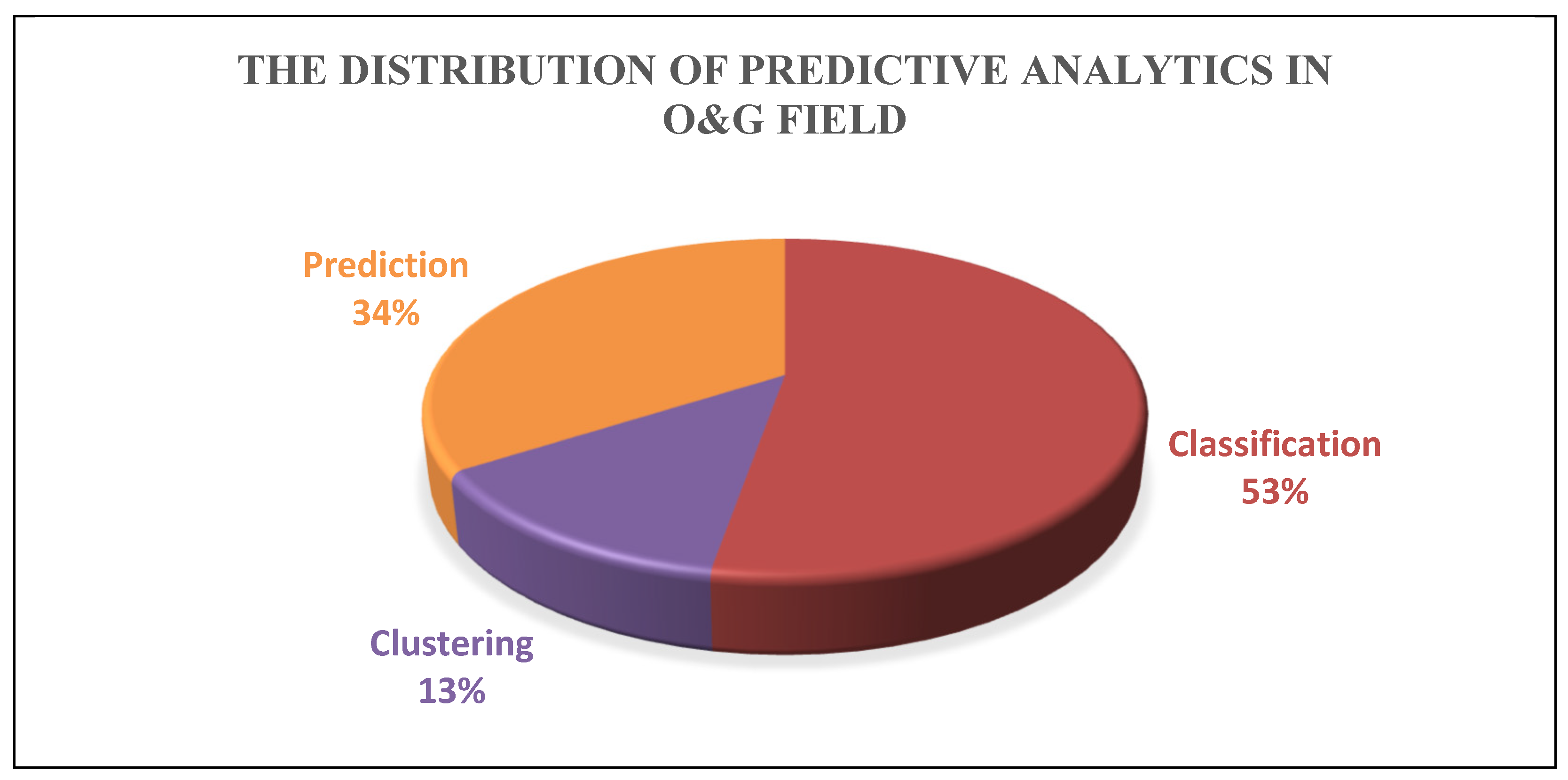
Figure 2. Total of Predictive Analytic Models in the O&G Field by Year.

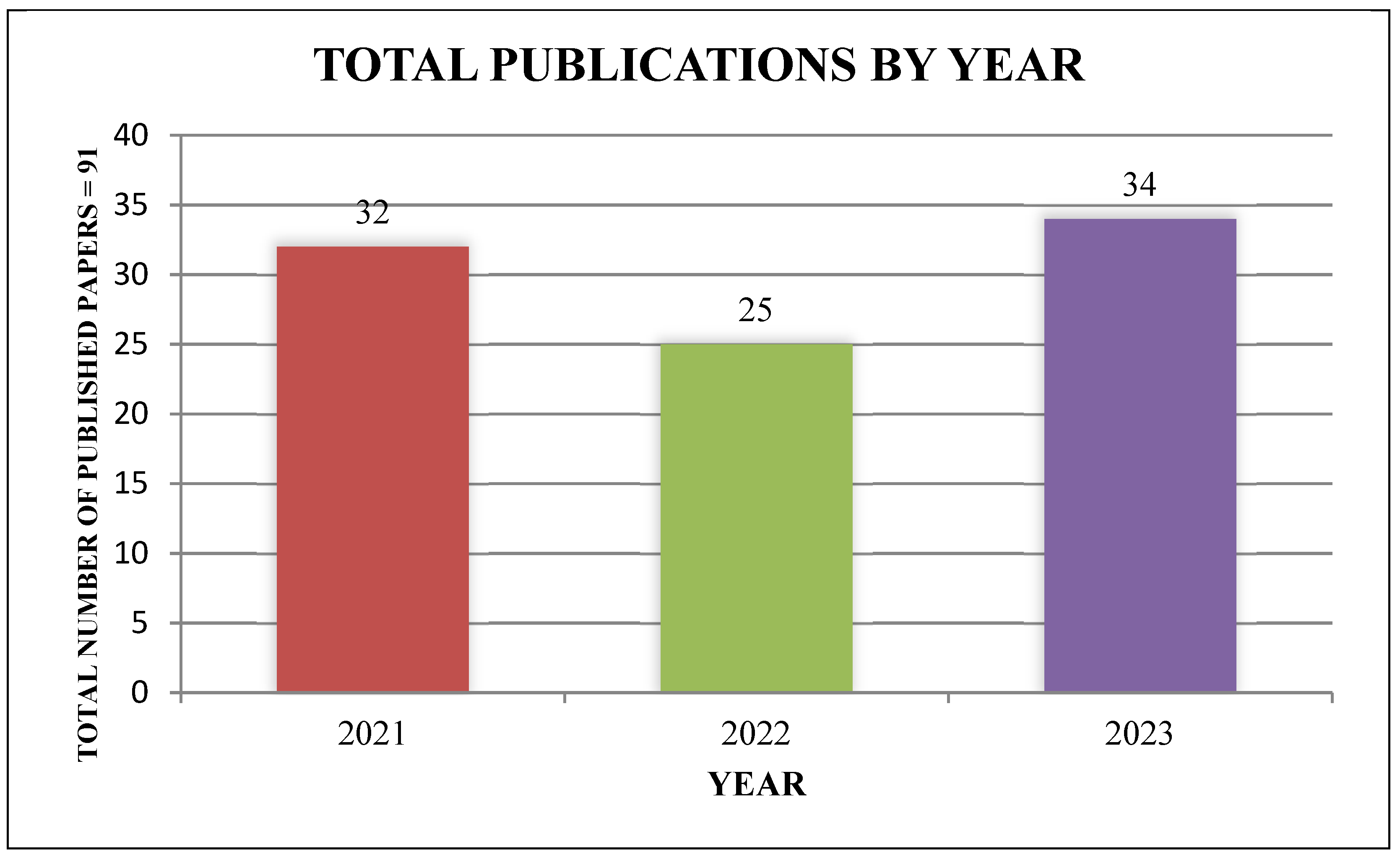
Figure 3. The architecture of Bi-LSTM [59].

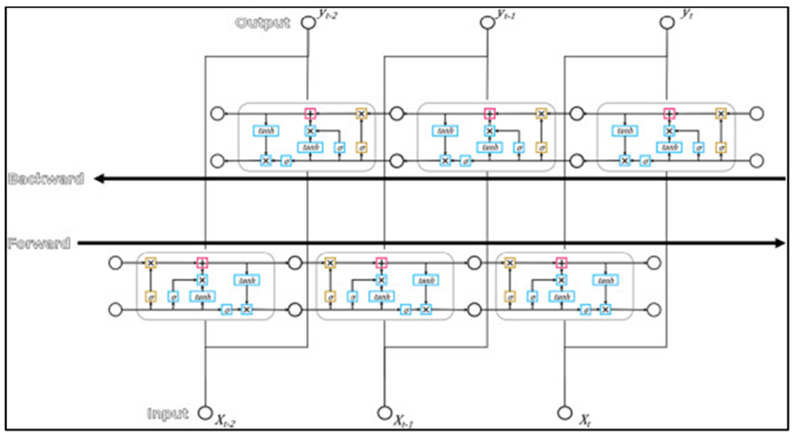
Table 1. A list of research articles on predictive analytics in O&G using ANN models.

Research	Applied AI models	Temporality	Field	Dataset	Class/ Clustering/ Prediction	Input Parameter	Output Parameter	Performance Metrics	Best Model	Advantages/Disadvantages
[43]	SVM, QPSO-ANN, WQPSO-ANN, LWQPSO-ANN	Non-temporal	Pipeline	Buried gas pipeline. 99 samples	Prediction	Pipe diameter (mm), Operating pressure (MPa), Cover depth (m), Crater width (m)	crater width	Map, R², MSE. RMSE, MAPE, MAE	LWQPSO-ANN	The proposed method outperformed the other method by more than 95%.
[45]	RF, KNN, ANN	Non-temporal	Wells	Middle East fields: for vertical wells 206 samples	Prediction	oil gravity (API), well perforation depth (Depth (ft), Surface temperature (ST (F)), well bottom-hole temperature (BT (F)), flowing gas rate (Qg (Mscf/day), flowing water rate (Qw (bbl/day), production tubing internal diameter (ID (inches) and wellhead pressure (Pwh (psia)).	vertical oil wells' flowing bottom-hole pressure Pwf (psia)	MSE, R²	ANN R² = 97% (training) and 93% (testing)	The suggested model has a much greater value than the other models.
[46]	ANN, LSB, Bagging	Non-temporal	Oil	Oil shale. 2,600 sample	Prediction	Air molar flowrate, illite silica, carbon, hydrogen content, feed preheater temp, air preheater temp	Petroleum output with CO2 emissions	RMSE	ANN Correlation correlations of 99.6% for oil yield and 99.9% for CO	The suggested model's precision outperformed the performance of the remaining models.
[47]	NB, KNN, DT, RF, SVM, ANN	Temporal	Oil	Ocean slick signature 769 samples	Classification	Data is confidential	Sea-Surface Petroleum Signatures	Accuracy, sensitivity, specificity, and predictive values	ANN Accuracy = 90%	The proposed model did not give significant results.
[44]	ANN, SVM, EL, and SVR	Non-temporal	Pipeline	Data is confidential	Classification	CO2, temperature, pH, liquid velocity, pressure, stress, glycol concentration. H2S, organic acid, oil type, water chemistry, hydraulic diameter	Corrosion defect depth.	MSE, R2	EL, ANN, and SVR	The proposed methods have a low error rate.
[48]	PLS, DNN, FPM, FP-DNN, FP-PLS	Non-temporal	Pipeline	long-distance pipelines 2,093 samples	Prediction	Mixed oil length, inner diameter, pipeline width, Reynolds number, equivalent length, and actual mixed oil length.	Mixed oil length.	RMSE	DNN RMSE = 146%	The error rate is not convincing and is the highest.
[49]	ANN, GA	Non-temporal	Crude Oil	ASPEN HYSYS V11 process simulator	Prediction	Well, feed flow rate, The pressure of gas products, Interstage gas discharge pressure, Isentropic efficiency of centrifugal compressor.	Enhance petroleum production.	R2	ANN	The performance enhancement of the variable using the ANN+GA has improved.
[50]	ANN	Non-temporal	Gas	Data is confidential. 104 samples	Prediction	Sulphur dioxide, methanol, and α-pinene.	The removal of gas-phase M, P, and H in an OLP-BTF and a TLP-BTF.	R2, MSE	ANN+PSO R2 > 99%	The proposed model is good, and the author suggested improving the model with real-world applications.
[51]	ANN, LSSVM, and MGGP	Temporal	Reservoir	Previous experimental and simulation studies 223 samples	Prediction	Height, dip angle, wetting phase viscosity, non-wetting phase viscosity, wetting phase density, non-wetting phase density, matrix porosity, fracture porosity, matrix permeability, fracture permeability, Injection rate, production time, and recovery factor.	gas-assisted gravity drainage (GAGD)	R2, RMSE, MSE, ARE, and AARE	ANN R2 = 97% RMSE = 0.0520	The ANN is outperformed the proposed method (MGGP = 89% (R2) and 0.0846 (RMSE)
[56]	GNN, Multivariate Time Series	Temporal	Transformer	DGA 1,408 samples	Clustering	H2, CH4, C2H6, C2H4, C2H2, CO, CO2	Power transformer fault diagnosis	Accuracy	MTGNN Accuracy = 92%	The model has proven to be effective in its application.
[30]	ANN, Multilayer Perceptron with Backpropagate	Non-temporal	Crude Oil	recent literature 172 samples	Prediction	Pressure (P)[Kpa], Temperature (T) [C], Liquid Viscosity (uL)[c.p.], Gas Viscosity (uG)[c.p.], Liquid Molar Volume (VL) [m3/kmol], Gas Molar Volume (VG) [m3/kmol], Liquid Molecular Weight (MWL) [kg/kmol], Gas Molecular Weight (MWG) [kg/kmol], and Interfacial Tension (o) [Dyne]	Diffusion Coefficient (D) [m2/s]	MSE, RMSE	Multilayer Perceptron with Backpropagate R2 for training is 88%, and testing is 89%	The suggested model has low accuracy. The hybrid does not improve the model's accuracy.
[52]	GA with backpropagation neural network	Temporal	Crude oil	crude oil gathering and transportation system. 509 samples	Prediction	The inlet temp of the combined system, outlet temp of the combined system, the inlet pressure of the combined system, outlet pressure of the combined system, inlet and outlet temp for the transfer station system, inlet and outlet pressure of the transfer station system, inlet and outlet of oil gathering wellhead system, treatment liquid volume, tot power consumption, and tot gas consumption	Energy = 99% Heat = 99% Power = 97%	R2	GA with backpropagation neural network	The model provides considerable results.
[53]	MLP, ANN	Temporal	Drilling	Egyptian General Petroleum Corporation (EGPC) 1,045 samples	Clustering and Classification	Epoch, age, formation, lithology, fields	Gas channels and chimneys prediction	RMSPE	MLP RMSE = 0.10	The proposed model has a lower error rate and outperforms the other method.
[54]	ELM, Elastic Net Linear, Linear-SVR, Multivariate Adaptive Regression Spline, Artificial Bee Colony, PSO, Differential Evolution, Simple Genetic Algorithm, GWO, xNES	Temporal	Shale gas	YuDong-Nan shale gas field	Prediction	The following minerals are quartz, calcite, dolomite, barite, pyrite, siderite, clay, and K-feldspar.	total organic carbon	R2, RMSE, MAE, MAPE, MARE, WI	DE+ELM = 0.497 (RMSE)	Acceptable results for ELM models hybrid with the proposed method except for GWO
[55]	MLP, Radial Basis Functions Neural Network	Temporal	Reservoir	Gullfaks” in the North Sea	Prediction	Injection rate for water, gas, and half-cycle time. Downtime.	Water alternating gas	Average absolute relative deviation (AARD)	MLP-LMA	The proposed model outperforms the other two proxy models and significantly reduces simulation time.

Table 2. Summary of the published research on deep learning models for predictive analytics in O&G.

Research	Applied AI models	Temporality	Field	Dataset	Class/ Clustering/ Prediction	Input Parameter	Output Parameter	Performance Metrics	Best Model	Advantages/Disadvantages
[60]	LSTM and GRU	Temporal	Reservoir	The Metro Interstate Traffic Volume Data set, The Appliances Energy Prediction Dataset, UNISIM-II-M-CO 301 samples	Prediction	Fluid production (oil, gas, and water), pressure (bottom-hole), and their ratios (water cut, gas-oil ratio, and gas-liquid ratio).	Oil production and pressure	MAE, RMSE, SMAPE	LSTM + Seq2Seq andGRU2architectures	The author suggested looking at another metaheuristic method, such as GA.
[58]	DCNN + LSTM, ANN, SVR, LSTM, RNN	Temporal	Pipeline	Real-time pipeline crack 90,000 data samples	Prediction	Pipeline condition, label, crack size, data length, sampling frequency, tube pressure	Natural gas pipeline crack	RMSE, MAPE, MAE, MSE, SNR	Optimized DCNN + LSTM Accuracy = 99.37%	The model showcases impressive performance.
[59]	LSTM, Bi-LSTM, GRU	Temporal	Well	West Natuna Basin dataset 11,497 samples	Prediction	GR, Vp, LLD, LLS, NPHI, and RHOB.	Well-log data imputation	MAE, RMSE, MAPE, R²	LSTM RMSE = 94%	The suggested model provides a greater accuracy.
[61]	KNN, SVM, XGBoost	Non-temporal	Transformer	DGA local power utilities and IEC TC 10 data set 1,530 samples	Classification	F7, F10, F17, F18, F19, F21, F24, F34, F36, and F40	Transformer Faults	Accuracy, Precision, Recall	KNN + SMOTE Accuracy: DGA = 98% IEC TC 10 = 97%	The proposed model outperforms the other model.
[62]	DL, DT, RF, ANN, SVR	Non-temporal	Reservoir	Sorush oil field and oil field of south Iran 7,245 samples	Prediction	Measure choke size (D64), wellhead pressure (Pwh), oil specific gravity (γo), and gas-liquid ratio (GLR).	Wellhead choke flow rates	RMSE, R²	DL R² = 99%	Compared to the other model, the accuracy of the suggested model is greater.
[63]	LSTM, GRU	Temporal	Reservoirs	UNISIM-IIH and Volve Oilfield 3,257 samples	Classification	oil, gas, water, or pressure	oil & gas forecasting	SMAPE, R²	GRU R² = 99%	The proposed model gives the highest accuracy.
[64]	Faster R-CNN_Res50, Faster R-CNN_Res50_DC, Faster R-CNN_Res50_FPN, With Edge detection, Cluster+Soft-NMS	Non-temporal	Well	Google Earth Imagery 439 samples	Clustering	Width and height	clustered oil wells	Precision, Recall, F1-measure, AP	Faster R-CNN with ClusterRPN = 71%	The proposed method’s running time higher than the other models and accuracy less than 90%.

Table 3. Published research on fuzzy logic and neuro-fuzzy modelling in predictive analytics in O&G.

Research	Applied AI models	Temporality	Field	Dataset	Class/ Clustering/ Prediction	Input Parameter	Output Parameter	Performance Metrics	Best Model	Advantages/Disadvantages
[69]	ANFIS, LSSVM-CSA, Gene Expression Programming	Non-temporal	Oil	Data is confidential	Prediction	Mixing time (min), MNP dosage (g/L), Oil concentration (ppm)	Oil adsorption capacity (mg/g adsorbent)	R², MPE, MAPE	LSSVM-CSA R² = 99%	The proposed method is outperformed by the other two models.
[67]	ANFIS, ANFIS+PCA	Non-temporal	Pipeline	Published studies. [70,71,72,73,74] 217 samples	Classification	Pipe dimension, burst pressure, pipe wall thickness, defect depth, defect width	Pressure	RMSE, MAE, R²	ANFIS+PCA R² = 99%	The proposed method outdistanced other models and significantly improved the model accuracy.
[41]	ANN, SVR, ANFIS	Non-temporal	Reservoir	CPG's waterflooding research group at the King Fahd University of Petroleum and Minerals in Saudi Arabia. 9,000 samples	Clustering	Reservoir heterogeneity degree (V), mobility ratio (M), permeability anisotropy ratio (kz/kx), wettability indicator (WI), production water cut (fw), and oil/water density ratio (DR).	The effectiveness of moveable oil recovery during a flood (RFM).	MAPE, MAE, MSE, R²	ANN	The proposed model has a better accuracy than the other models and saves the runtime and cost.
[68]	RF, Fuzzy C Means, Control Chart	Temporal	Well	3W dataset 50,000 samples	Classification	P-PDG, T-PDG, and T-PCK, grouping three classes (“normal,” “high fault,” “high fault”)	failure detection applications	Total Variance	Control chart + RF Specificity = 99% Sensitivity = 100%	The proposed method has shown higher sensitivity and specificity.

Table 4. Summary of the literature on the application of decision tree, random forest, and hybrid models.

Research	Applied AI models	Temporality	Field	Dataset	Class/ Clustering/ Prediction	Input Parameter	Output Parameter	Performance Metrics	Best Model	Advantages/Disadvantages
[77]	KNN, DT, RF, NB, AdaBoost, XGBoost, and CatBoost	Non-temporal	Pipeline	National Science Foundation (NSF) Critical Resilient Interdependent Infrastructure Systems and Processes (CRISP) 959 samples	Classification	Pipe diameter, wall thickness, defect depth, defect length, yield strength, ultimate tensile strength, operating pressure	Failure risk pipeline	Precision, Recall, Mean accuracy	XGBoost Accuracy = 85%	The proposed model needs to have an improvement in accuracy.
[78]	LR, RF, SVM, XGBoost, ANN	Non-temporal	Reservoir	Well-log data from North China 1,500 samples	Classification	CAL, CNL, AC, GR, PE, RD, RMLL, RS, SP, DEN, DTS, and SP	Shear wave travel time (DTS)	R²	XGBoost R² = 99% (Training) and 96% (Testing)	The best model is significant.
[37]	ELM, SVM, KNN, DT, RF, EL	Temporal	Transformer	DGA 542 samples	Classification	C2H2, C2H6, CH4, H2	Power transformer fault	Mean Accuracy	EN Accuracy = 78% (Training) and 84% (Testing)	The proposed model’s performance accuracy is not above 90%.
[79]	DT, LDA, GB, Ensemble Tree, LGBM, RF, KNN, NB, LR, QDA, Ridge, SVM-Linear	Non-temporal	Transformer	DGA 3,147 samples	Classification	C2H2, C2H4, C2H6, CH4	Transformer fault	Accuracy, AUC, Recall, Precision, F1-Measure, Kappa, MCC, and Time-taken.	QDA Accuracy = 99.29%	The proposed method has the best accuracy classifier model.
[80]	DT	Temporal	Well	KG Composition 180 samples	Classification	KG, including hydrogen (H2), methane (CH4), ethane (C2H6), ethylene (C2H4), and acetylene (C2H2)	Incipient Faults in Transformer Oil.	Accuracy. AUC	DT Accuracy = 62.9%	The current model exhibits potential, and we recommend exploring opportunities for refinement to enhance its overall efficacy.
[81]	LR, DT, RF, KNN, SMOTE, XAI, SHAP, LIME	Non-temporal	Well	3W 1,984 samples	Classification	P-PDG, P-TPT, T-TPT, P-MON- PCK, T-JUS, PCK, P-JUS- CKGL, T-JUS- CKGL, QGL	Detect anomalies in oil wells	accuracy, recall, precision, F1-score, and AUC	RF Accuracy = 99.6%, recall = 99.64%, precision = 99.91%, F1-score = 99.77%, and AUC = 1.00%.	The result of the proposed model is significant.
[82]	LDA, QDA, Linear SVC, LR, DT, RF, Adaboost	Temporal	Well	3W dataset 2,000 samples	Classification	P-PDG, P-TPT, T-TPT, P-MON-CKP, T-JUS-CKP	Undesirable events	F1-score, Accuracy	DT Accuracy = 97%	The feature selection did not boost accuracy, and training time was increased with feature selection. The proposed method struggles with class 2 due to limited data and mismatched labels from calculated features.
[106]	DT, ANN, SVM. LR. KNN, NB	Temporal	Pipeline	external defects of pipelines in the United States 7,000 samples	Classification	Consider the defect's length, breadth, and pipeline's nominal thickness.	Classification for pipeline corrosion	Accuracy	DT Accuracy = 99.9%	The accuracy of the model is significant to the research.
[85]	LGBM, CatBoost, XGBoost, RF, and NN	Temporal	Crude oil	WTI crude oil 2,687 samples	Classification	Gold, silver, crude oil, platinum, copper, the dollar index, the volatility index, and the euro Bitcoin: Green Energy Resources ESG.	Oil prices	accuracy, and AUC	LGBM and RF	The proposed method indicates superiority over traditional methods.
[86]	GB, RF, MLR	Non-temporal	Reservoir	Shale gas reservoirs 1,400 samples	Prediction	Horizontal wellbore length, hydraulic fracture length, reservoir length, SRV fracture porosity, permeability, spacing, and pressure, total production time.	CO2	MSE	RF	The best method is surpassing the other method in ML.
[87]	RF, ANN, FN	Temporal	Drilling	Real time Well-1 data 8,983 samples	Classification	Standpipe pressure (SPP), weight-on-bit (WOB), rotary speed (RS), flow rate (Q), hook load (HL), rate of penetration (ROP), and rotary speed (RS).	torque and drag (T&D)	R and AAPE	RF	The proposed model has higher accuracy than the other two models.
[88]	RF	Temporal	Reservoir	2D simulation in STARS 240 samples	Prediction	Formation compressibility, volumetric heat capacity, rock, water, oil, and thermal conductivity.	Shale barrier	R2, RMSE	RF	The author suggested that incorporating more training data and features can improve the proposed method.
[89]	RF, XGBoost, SVM, LGBM	Non-temporal	Pipeline	full-scale corroded O&G pipelines 314 samples	Prediction	Depth, length, and width of corrosion defects, wall thickness, pipe diameter, steel grade, and burst pressure.	Corroded pipelines of gas and oil of burst pressure.	R2, RMSE, MAE, MAPE	XGBoost R2 = 99% (training) and 98% (testing)	The hybrid proposed model has significantly higher prediction accuracy.
[90]	XGBoost, SVM, NN	Non-temporal	Pipeline	OLGA data and PIG data 1,700 samples	Classification	Geometrical variables: Odometry begins, ends, latitude, longitude, elevation, and bar length.Water volumetric flow rate, continuous velocity, water film shear stress, hold-up, flow regime, pressure, total mass and volumetric flow rates inclination, temperature, section area, gas mass and volumetric flow rates, gas velocity, wall shear stress, total water mass and flow rate (including vapor),	Internal Corrosion in Pipeline Infrastructures	Mean accuracy and F1 score	XGBoost Accuracy = 62%	The proposed model needs an improvement in the accuracy.
[91]	RF, CatBoost	Non-temporal	Pipeline	Crude oil dataset 3,240 samples	Prediction	stream compositions (nO2, nH2S, nCO2), pressure (P), velocity (v), and temperature (T)	Corrosion rates	R2, MSE MAE RMSE	CatBoost Accuracy = 99.9% training and testing	The proposed model’s accuracy is outperformed the other models.
[32]	RF, KNN	Temporal	Transformer	DGA 11,400 samples	Classification	Acetylene (𝐶𝐶2𝐻𝐻2), Ethylene (𝐶𝐶2𝐻𝐻4), Ethane (𝐶𝐶2𝐻𝐻6), Methane (𝐶𝐶𝐻𝐻4), and Hydrogen (𝐻𝐻2)	Identify transformer fault types	Mean accuracy	KNN Accuracy = 88%	The proposed model needs an improvement on the accuracy.
[92]	XGBoost, CatBoost, LGBM, RF, deep MLN, DBN, CNN	Non-Temporal	Crude-oil	Previous studies on CO2-oil MMP databank 310 samples	Classification	Crude oil fractions (N2, C1, H2S, CO2, C2-C5), average critical injection gas temperature (Tcave), reservoir temperature (Tres), molecular weight of C5+ fraction (MWc5+).	Estimating the MMP of CO2-crude oil system	ARD, AARD, RMSE, MPa, SD	CatBoost R2 = 99%	The proposed model confirms its superiority against other models.
[93]	DF + K-means, RF, SVM, DNN, DF	Non-temporal	Lithology	Lithology dataset from Pearl River Mouth Basin 601 samples	Classification	Sandstone (S00), siltstone (S06), grey siltstone (S37), mudstone (N00), sandy mudstone (N01), and limestone (H00).	lithology identification	Precision, recall and Fβ	DF + K-means Accuracy = 90%	The baseline method cannot predict well on the minority class, small amount data label, error labelling, and noisy data
[94]	GSK- XGBoost	Temporal	Transformer	DGA 128 samples	Classification	ammonia, acetaldehyde, acetone, ethylene, ethanol, and toluene	Ethanol, Ethylene. Ammonia, Acetaldehyde. Acetone and Toluene	Accuracy, precision, recall, f-measurement, beta-factor	GSK- XGBoost Mean accuracy = 50%	The computational time is increased and the proposed model’s accuracy after use the develop method does not exceed to 90%
[95]	LGBM, XGBoost, RF, LR, SVM, NB, KNN, DT	Non-temporal	Transformer	DGA 796 samples	Classification	H2, CH4, C2H2, C2H4, and C2H6	fault type classification	accuracy, precision, recall, and F1 scores	LGBM Accuracy = 87.06%	The model demonstrates a high level of competence.
[5]	Adaboost, RF, KNN, NB, MLP, SVM	Non-temporal	Drilling	Drill bit type in Norwegian Wells 4,312 samples	Classification	Depth as Measured (DT), Ve rtical True Depth (TVD) Penetration Rate (ROP) Bit weight (WOB) Minutes per round (RPM) torque (TQ) SPP, or standpipe pressure Mud mass (MW) Rate of Flow in (FR) Totalized Gas (TG) Bit kind (BT) Bit Quantity (BS) DEXP stands for D-exponent. Area of total flow (TFA) Specific Mechanical Energy (MSE) Cut Depth (DC) Aggressiveness of Drill Bit (DBA).	Drill Bit Selection	Accuracy, Precision, F1 Score, Recall, MCC, G-mean	RF Accuracy = 97% (Training) and 91% (Testing)	The proposed method is more reliable, stable, and accurate than previous models.
[96]	RF	Temporal	Well	3W 1,984 samples	Classification	P-PDG, P-TPT, P-PCK, T-PCK, P-JUS-CKGL, T-JUS-CKGL, and gas lift flow	Early fault detection	Accuracy, Faulty-normal accuracy (FNACC), Real faulty-normal accuracy (RFNACC)	RF Accuracy = 94%	The proposed method gives a good result for detecting the early fault.
[83]	One Directional, CNN, RF, GNN, QDA	Temporal	Well	3W 1,984 samples	Classification	P-PDG, T-TPT, P-MON-CKP, T-JUS-CKP, P-JUS-CKGL, QGL.	Anomalous events in oi	Accuracy, precision, recall, F1 score	RF Mean accuracy = 95%	Time windows increase
[84]	RF, PCA	Temporal	Well	3W 1,984 samples	Classification	P-PDG, P-TPT, T-TPT, P-MON-CKP, T-PCK	Anomalous events in oil wells	Accuracy	RF+PCA Accuracy = 90%	The proposed method’s accuracy > 95% for all classes.
[97]	SVM, LOF, RF	Temporal	Reservoir	Well log data. 37 samples	Clustering	Depth, gammar ray, shallow resistivity, deep resistivity, neutron, density, CALI, DTS	Sonic (DTC)	R2	KMeans+RF R2=0.92 to R2=0.98	The proposed hybrid approach outperformed several baseline methods.
[98]	RF	Temporal	Well	Field and well-scale data from a significant US 934 samples	Clustering	API, On-stream date, Surface latitude and longitude, Formation thickness, TVD, Lateral length, Total proppant mass, Total injected fluid volume, API gravity, Porosity, Permeability, TOC, VClay, Oil production rate, Gas production rate, Water production rate, GPI, Frac fluid.	barrel of oil equivalent (BOE)	RMSE, R2	RF RMSE: Train = 7.25% Test = 17.49%	The proposed method needs an improvement of accuracy, and the model is overfitting.
[100]	RF with Analog-to-digital converters	Non-temporal	Well	Well-logging dataset 100 samples	Clustering	neutron (CNL), gamma ray (GR), density (DEN), and compres sional slowness (DTC)	well-logging data generation	RMSE, MAE, MAPE, MSE	RF with Analog-to-digital converters RMSE = 9%, MAE = 6%, MAPE = 0.031% MSE = 86%	The proposed model needs an improvement on the accuracy for clustering.
[107]	RF	Temporal	Transformer	DPM1 and DPM2 for DGA 2,123 samples	Classification	H2 (hydrogen), CH4 (methane), C2H2 (acetylene), C2H4 (ethylene), C2H6 (ethane), CO (carbon monoxide), CO2 (carbon dioxide), O2 (oxygen) and N2 (nitrogen)	transformer fault diagnosis	Accuracy	RF Accuracy = DPM1 = 96.2% DPM2 = 96.5%	For the evaluation dataset, the suggested models diagnose errors with a satisfactory level of performance.
[101]	KNN, Multilayer Perceptron Neural Network, multiclass SVM, XGBoost	Temporal	Pipeline	climate change data 81 samples	Classification	location, time, pipeline age, pipeline material, temperature, humidity, and wind speed.	gas pipeline	Accuracy, Precision, Recall, F1-Score	XGBOOST Accuracy = 92%	The model outperformed other models however it needs to have an improvement.
[102]	LogitBoost, GBM, XGBoost, AdaBoost, KNN	Temporal	Well	Lithofacies and Well-log dataset 399 samples	Classification	GR, CALI, NEU, DT, DEN, RES DEP, RES SLW, PHIT and SW	lithofacies predictions	total percent of correct (TPC)	XGBoost TPC = 97%	The model gives significantly results to the proposed method.
[103]	recursive feature elimination and particle swarm optimization-AdaBoost	Non-temporal	Pipeline	Changshou-Fuling-Wulong-Nanchuan (CN) gas pipeline dataset 3,986 samples	Clustering	Landslide susceptibility Area, Percentage, and Historical landslides.	long-distance pipelines	Accuracy, sensitivity, precision. F1 score	recursive feature elimination and particle swarm optimization-AdaBoost Accuracy = 90% (Training) and 83% (Testing)	The proposed model needs an improvement on the accuracy.
[108]	LSTM, AdaBoost, LR, SVR, DNN, RF, adaptive RF	Temporal	Crude Oil	United states’ Energy Information Administration Brent COP data	Prediction	Shape, location, scale	crude oil price (COP)	MAPE, MSE, RMSE, MAE, EVS	Adaptive RF MAPE = 112.31%; MAE = 52%; MSE = 53%; RMSE =73%; R2 = 99%; EVS = 99%	The proposed model is outperformed than others however the running time is highest than the other models
[105]	RF, DT	Temporal	Drilling	Data is confidential	Prediction	WOB, torque, standpipe pressure, drill string rotation speed, rate of penetration, and pump rate.	Rock porosity	R2, AAPE, VAF	RF Accuracy = 99% training and 90% testing	The model stands out for its exceptional performance.
[104]	BayesOpt-XGBoost, XGBoost	Non-temporal	Reservoir	The Equinor Volve Field Datasets 2,853 samples	Classification	DT, GR, NPHI, RT, and RHOB.	vshale, porosity, horizontal permeability (KLOGH), and water saturation.	RMSE, MAE	BayesOpt-XGBoost Accuracy = 93%, precision score = 98%, recall score = 86%, and combined F1-score = 93%	The proposed method does not robust enough to predict all the output.
[99]	RF, KNN, NB, DT, NN	Temporal	Transformer	New O&G decommissioning dataset from GitHub 1,846 samples	Classification	Size, diameter, length, metal, plastic, concrete, residues, position, and decision of the company, organization name, type, technical, safety, sociological, environmental, cost, weight,	predictive decommissioning options	Recall, Precision, F1-score, AUC	RF Accuracy: Full features = 80.06% Redundant removed = 80.66%	The proposed method needs an improvement.

Table 5. Previous research published on interrelated AI model for predictive analytics in O&G.

Research	Applied AI models	Temporality	Field	Dataset	Class/ Clustering/ Prediction	Input Parameter	Output Parameter	Performance Metrics	Best Model	Advantages/Disadvantages
[111]	MLR, SVR, GPR	Non-temporal	Gas	M6COND and M6GAS 129 samples	Clustering	Condensate-gas ratio, total horizontal lateral length, gas saturation, total organic carbon content, cluster and stage counts, proppant amount, fluid volume, and total horizontal lateral length.	Gas well.	RMSE, R²	GPR	The proposed method needs improvement in the accuracy.
[112]	XGBoost, ANN, RNN, MLR, PLR, SVR, DTR, RFR	Temporal	O&G production	Saudi Aramco of five well reservoirs 1,968 samples	Classification	Location, contact, average permeability, volume, production, pressure ratio between the wellhead and bottomhole, and production.	Oil, gas, and water.	R2, MAE, MSE, RMSE	RNN R²: Oil = 98% Gas = 87% Water = 92%	The proposed model needs an improvement on the output.
[113]	MLP, RF, SVR	Non-temporal	Pipeline	History record of pipeline failure 149,940 samples	Classification	Effects of transportation disruptions on safety and health, the environment and ecology, and equipment maintenance.	Natural gas pipeline failure.	RMSE, MAE. MSE. R²	RF	The proposed methods have shortest computing time and best fitting results.
[114]	SVM	Non-temporal	Reservoir	MMP data 147 samples	Classification	reservoir temperature, oil composition and gas composition	Minimum miscibility pressure of CO2 and crude oil.	MSE	SVM- POLY kernel	The proposed model’s accuracy is outperformed the other models.
[19]	RF, ARN, LSTM, Independently Recurrent Neural Network, component-wise gradient	Temporal	Well	3W 1,984 samples	Classification	P-PDG, T-TPT, P-TPT, Initial Normal, Steady state, transient	Oil wells production.	Accuracy, precision, recall, f-measure	ARN Accuracy = 96% Precision = 88% Recall = 84% F-measure = 85%	The proposed model is not robust because misclassification for undesirable events for type 3 and type 8.
[115]	SVR-GA-PSO, SVR, SVR-GA, SVR-FA, SVR-PSO, SVR-ABC, SVR-BAT, SVR-COA, SVR-GWO, SVR-HAS, SVR-ICA, SVR-SFLA	Temporal	Pipeline	Iranian Oilfields 340 samples	Classification	Onshore oil and gas pipelines: Pit depths, exposure times, pitting start times, operational pressures, temperatures, water cuts, redox potentials, resistivities, pH, concentrations of sulfate and chloride ions, production rates.	Carbon steel corrosion rate	MSE, RMSE, MAE, EVS, R2, RSE	SVR-GA-PSO R2 = 99% RMSE = 0.0099 MSE = 9.84*10−5 MAE = 0.008 RSE = 0.001 EVS = 0.955	The proposed model shows a good result than others
[116]	BLR, PBBLR, ANN, Gradient Boosting DT	Non-temporal	Pipeline	SCADA (Supervisory Control and Data Acquisition) system 728 samples	Prediction	Diameter, Reynolds number, transportation distance, mixed oil length.	Actual mixed oil length	RMSE, MAE, R2	PBBLR	The proposed model is required to improve accuracy

Table 6. Previous study on statistical model for predictive analytics modelling in O&G.

Research	Applied AI models	Temporality	Field	Dataset	Class/ Clustering/ Prediction	Input Parameter	Output Parameter	Performance Metrics	Best Model	Advantages/Disadvantages
[119]	SARIMA, LSTM, AR	Temporal	Transformer	DGA 610 samples	Prediction	H2, CH4, C2H4, C2H6, CO, CO2, and total hydrocarbon (TH).	dissolved gas concentration	ARE	SARIMA	The proposed method provides a good means.
[120]	LSTM, ARIMA	Temporal	Wells	Longmaxi Formation of the Sichuan Basin 3,650 samples	Prediction	Date, Daily production	Shale gas production	MAE, RMSE, R²	LSTM Accuracy = 0.63%	The accuracy of the model needs more improvement.
[121]	GM, FGM, DGGM, ARIMA, PSOGM, PSO-FDGGM	Temporal	Gas	quarterly production of natural gas in China	Prediction	Training period, natural gas production	Natural gas production	MAPE	PSO-FDGGM MAPE = 3.19%	The model's performance is noteworthy and reliable.

Table 7. Previous work on the application of ML models for predictive analytics modelling in O&G fields.

Research	Applied AI models	Temporality	Field	Dataset	Class/ Clustering/ Prediction	Input Parameter	Output Parameter	Performance Metrics	Best Model	Advantages/Disadvantages
[122]	Multivariate Empirical Mode Decomposition with Genetic Algorithm, LSSVM-GA and LSSVM-PSO	Non-temporal	Crude oils	Bubble point pressure & oil formation volume factor. 638 samples	Clustering	Temperature (T), oil gravity (API), gas specific gravity (γg), and solution gas oil ratio (Rs).	bubble point pressure & oil formation volume factor of crude oils	RMSE	MELM-PSO	The hybrid proposed model outperform the empirical method.
[124]	PCA, SVM, LDA	Temporal	Oil	Real time oil samples 30 samples	Classification	pore size remains the same, the capillary flow rate (l2/t) is a function of interfacial properties (γLG and θ) and viscosity (μ).	Oil types	Accuracy	SVM Accuracy = 90%	The proposed model needs an improvement on the accuracy because the accuracy < 95%.
[125]	MLP-PSO, MLP-GA	Non-temporal	Well-log	Three wellbores drilled. 2,2323 samples	Prediction	Depth DTC (Vp) DTS (Vs) RHOB (ρ) Pp	probable depth of casing collapse	R^2, RMSE	MLP-PSO	The proposed model outperformed the other models’ accuracy.
[126]	LSSVM-COA, LSSVM-PSO, LSSVM-GA, MLP-COA, MLP-PSO, MLP-GA, LSSVM, MLP	Non-temporal	Drilling	305 drilled wells in the Marun oil field 2,820 samples	Prediction	Northing, easting, depth, meterage, formation type, hole size, WOB, flow rate, MW, MFVIS, retort solid, pore pressure, drilling time, fracture pressure, fan 600/fan 300, gel10min/gel10s, pump pressure, RPM.	severity of mud loss	R2 and RMSE	MLP-GA RMSE = 93%	The accuracy of the proposed model can be improved.
[127]	Hybrid-Physics Guided-Variational Bayesian Spatial- Temporal neural network	Temporal	Gas	Natural gas 600 samples	Prediction	Geometry size, location of release point, release diameter, released gas, volumetric release rate, release during, release duration, location of sensor	Natural gas concentration	R²	Hybrid_PG_VBSTnn R² = 99%	The proposed integration enhances the spatiotemporal forecasting performance.
[123]	CNN, Linear SVM, Gaussian SVM, SVM+CNN	Temporal	Gas	Leakage dataset 1,000 samples	Classification	Methane, Ethane, Propane, Isobutane, Butane, Helium, Nitrogen, Hydrogen Sulphide, Carbon Dioxide	Gas Pipeline Leakage Estimation	Accuracy	SVM Accuracy = 95.5%	The model stands out for its exceptional performance.
[128]	LSTM, OCSVM	Temporal	Well	3W 1,984 samples	Classification	P-PDG P-TPT T-TPT P-MON-CKP T-JUS-CKP	Identify two types of faults	Recall, Specificity, Accuracy	OCSVM Accuracy = 91%	The use of feature selection did not improve the classifier accuracy, the proposed model is not robust enough to classify 2 types of wells.
[7]	Ordered Nearest Neighbors, Weighted Nearest Neighbors, LDA, QDA	Temporal	Well	3W 1,984 samples	Classification	P-PDG, P-TPT, T-TPT, P-MON-CKP, T-JUS-CKP, CLASS	Predicting flow instability	Recall, Specificity, Accuracy	ONN Accuracy = 81%	The author suggested to investigate another metaheuristic method.
[130]	CNN, SVM and SVM+CNN	Temporal	Pipeline	Leakage dataset 1,000 samples	Prediction	Length, outer diameter, wall thickness, location in the model	Prediction in tight sandstone reservoirs	Accuracy	SVMCNN model, achieved 95.5%	The proposed method is outperformed other method.
[129]	DT, SVM	Non-temporal	Reservoir	high-resolution FMI data	Classification	Response of logging, Pyroclastic lava, Normal pyroclastic rock Sedimentary pyroclastic rock	Lithologic classification of pyroclastic rocks	Accuracy	SVM Accuracy = 98.6%	The proposed model is higher than 95%.
[131]	BAE-OCSVM, CAE-OCSVM, LSTM-AE- OCSVM, RD-OCSVM, RF-OCSVM, PCA-OCSVM, VAE-OCSVM, LSTM-AE-IF	Temporal	Gas	Data from SCADA 9,980 samples	Classification	Diameter, Wall thickness, length	Leakage of natural gas	AUC, Accuracy, F1 score, precision, TPR, FPR	LSTM- AE-OCSVM Accuracy = 98%	The best model achieves higher accuracy and author suggested to use abnormal data for future work.
[63]	LSTM, GRU	Temporal	Reservoirs	UNISIM-IIH and Volve oilfield 3,257 samples	Classification	Oil, gas, water, or pressure	oil & gas forecasting	SMAPE, R²	GRU R² = 99%	The proposed model gives a highest accuracy.
[133]	OCSVM, LOF, Elliptical Envelope, and Autoencoder with feedforward and LSTM	Temporal	Well	3W 1,984 samples	Classification	P-PDG, P-TPT, T-TPT, P-MON-CKP, T-JUS-CKP, P-JUS-CKGL, T-JUS-CKGL, QGL, Label vector	Fault detection	F1 score	LOF F1 score = 85%	The proposed method need an improvement on the accuracy.
[132]	K-Means Clustering and KNN	Temporal	Reservoirs	Antrim, Barnett, Eager Ford, Woodford, Fayetteville, Haynesville, Marcellus 55,623 samples	Clustering	Well location, well depth, well length, and production starting year	EUR predictions	R²	K-MC R² = 0.18	The proposed model outperformed the other models using average fitting parameters.
[134]	GS-GMDH	Non-temporal	Well	oil fields located in the Middle East 2,748 samples	Prediction	Laterolog (LLS), photoelectric index (PEF), compressional wave velocity (Vp), porosity (NPHI), gamma ray (spectral) (SGR), density (RHOB), gamma ray (corrected) (CGR), shear wave velocity (Vs), caliper (CALI), resistivity (ILD), and sonic transit time (DT).	Pore Pressure	RMSE, R², MSE, SI, ENS	GS-GMDH RMSE = 1.88 psi and R² = 0.9997	The proposed method shows the higher accuracy.
[135]	RF, Gradient Boosting Regressor , bagging, CNN, KNN, Deep Hierarchical Decomposition	Temporal	Reservoir	Geological data 180 samples	Classification	Porosity, fracture porosity, fracture permeability, rocky type, net gross, matrix permeability, water relative permeability, formation volume factor, rock compressibility, pressure dependence of water viscosity, gas density, water density, vertical continuity, relative permeability curves, oil-water contact, fluid viscosity.	Oil production, water production, water injection, and liquid production	MAE, SMAPE	Deep Hierarchical Decomposition MAE: OP = 0.76%	The proposed method has decreased the computational speed.
[136]	M5P tree model, RF, Random Tree, Reduced error pruning tree, GPR, SVM, and MARS	Non-temporal	Gas	Coriolis flow meter 201 samples	Classification	wet gas flow rate (kg/h) and absolute gas humidity (g/m3)	estimation of the dry gas flow rate (kg/h)	RMSE, MAE, LMI, WI	GPR-RBKF MAE = 163.3266 kg/h,RMSE = 483.1359 kg/h, CC = 0.9915 for the testing data set	The best model superior rather than the other models and the author suggested to explore other soft-computing method.

Disclaimer/Publisher’s Note: The statements, opinions and data contained in all publications are solely those of the individual author(s) and contributor(s) and not of MDPI and/or the editor(s). MDPI and/or the editor(s) disclaim responsibility for any injury to people or property resulting from any ideas, methods, instructions or products referred to in the content.

© 2024 by the authors. Licensee MDPI, Basel, Switzerland. This article is an open access article distributed under the terms and conditions of the Creative Commons Attribution (CC BY) license (http://creativecommons.org/licenses/by/4.0/).

Copyright: This open access article is published under a Creative Commons CC BY 4.0 license, which permit the free download, distribution, and reuse, provided that the author and preprint are cited in any reuse.

Downloads

187

Views

Comments

Subscription

Notify me about updates to this article or when a peer-reviewed version is published.

MDPI Initiatives

Important Links

Choose an area of interest and we will send you notifications of new preprints at your preferred frequency.

Disclaimer