Submitted:
02 May 2024
Posted:
07 May 2024
You are already at the latest version
Abstract
Brain tumors are frequently classified with high accuracy using convolutional neural networks (CNNs) and better comprehend the spatial connections among pixels in complex pictures. Due to their tiny receptive fields, the majority of deep convolutional neural network (DCNN)-based techniques overfit and are unable to extract global context information from more significant regions. While dilated convolution retains data resolution at the output layer and increases the receptive field without adding computation, stacking several dilated convolutions has the drawback of producing a grid effect. To handle gridding artifacts and extract both coarse and fine features from the images, this research suggests using a dilated parallel deep convolutional neural network (PDCNN) architecture that preserves a wide receptive field. To reduce complexity, initially, input images are resized and then grayscale transformed. Data augmentation has since been used to expand the number of datasets. Dilated PDCNN makes use of the lower computational overhead and contributes to the reduction of gridding artifacts. By contrasting various dilation rates, the global path uses a low dilation rate (2,1,1), while the local path uses a high dilation rate (4,2,1) for decremental even numbers to tackle gridding artifacts and extract both coarse and fine features from the two parallel paths. Using three different types of MRI datasets, the suggested dilated PDCNN with the average ensemble method performs better. The accuracy provided by the Multiclass Kaggle dataset-III, Figshare dataset-II, and Binary tumor identification dataset-I is 98.35%, 98.13%, and 98.67%, respectively. In comparison to state-of-the-art techniques, the suggested structure improves results by extracting both fine and coarse features, making it efficient.
Keywords:
Brain tumor classification
; data augmentation
; receptive field
; grid effect
; multiscale dilated parallel convolution
; machine learning classifiers
1. Introduction
The growth that may adversely impact a person's life is a brain tumor, which can appear in the tissues enclosing the brain or skull. Two characteristics can identify a benign or malignant growth. While secondary tumors, also referred to as brain metastasis tumors, are typically formed from tumors outside the brain, primary cancers start inside the brain. Meningioma, pituitary adenomas, and gliomas are the three most common primary brain tumors. The brain, and spinal cord membrane layers, are the origin of meningioma, a tumor that grows slowly. Cancerous cells that arise in the pituitary gland are referred to as pituitary adenomas [1]. The brain tissue is compressed by the irregular growth of these tumors. Malignant tumors, in comparison with benign tumors, grow unevenly and damage the tissues around them. Surgical techniques are frequently employed in the treatment of brain tumors [2]. Because MRI is non-interfering, it is preferred over computed tomography (CT), positron emission tomography (PMT), and x-rays [3]. It is estimated that 79,340 Americans aged 40 and older will be diagnosed with a primary brain tumor by 2023. It is estimated that one million Americans suffer from primary brain tumors; of these, 72% are benign tumors and 28% are malignant. The adults with primary brain tumors typically have meningioma (46.1%), glioblastoma (16.4%), and pituitary tumors (14.5%) [4,5]. Biopsies are taken for analysis after the tumor is found using standard medical techniques like MRI. The first test used in medicine to find cancer is the MRI [6,7]. Two MRI pictures of two distinct brains are shown in Figure 1.
As the number of patients has grown, individually analyzing these images has become laborious, disorganized, and frequently incorrect. A computer-aided diagnostic technique that concludes the expense of brain MRI identification needs to be developed to ease this limitation. Many attempts have been made to create an extremely effective and trustworthy method for classifying brain tumors automatically. Conventional approaches to machine learning rely on handmade qualities, which increases the cost and limits the durability of the solution. But occasionally, models of supervised learning can perform better than unsupervised learning strategies, leading to an overfitted framework that is inappropriate for another large database. These challenges underscore the significance of creating a machine learning-based, fully automated system for classifying brain tumors.
CNN's architecture is based on a neural network known as the deep learning model, which excels at image recognition and classification. [9,10]. The receptive field in CNN is too tiny to produce excellent precision [11]. A large receptive field of the convolution kernel would help enhance the efficiency of the classification techniques because the fixed size of the sliding window in CNN misses out on utilizing techniques like convolution, pooling, and flattening. The recommended model's parameters possess the ability to acquire characteristics extracted from the images. While hyperparameters are focused on, recent iterations of CNN models have yet to focus much on them. Another important consideration is CNN's local feature collection. Furthermore, because of the limited quantity of the kernel, sharply raising the dilation rate could exacerbate feature collection failures and hinder small object detection [12]. High dilation rates may impact tiny object detection. As a result, the dilation rate has been gradually decreased in this suggested model. By doing this, the dilated feature map's sparsity has decreased and more data can be extracted from the investigated region.
Using publicly available Kaggle and Figshare datasets, this work aims to develop a fully autonomous dilated PDCNN with an average ensemble model for brain tumor classification [8,13,14]. This article suggests an architecture for the detection and classification of brain tumors that consists of two synchronously dilated DCNNs. Because convolutions are accurate and time-efficient processes, the dilated PDCNN with an average ensemble model performs more quickly than the conditional random field (CRF)-based methods. The recommended dilated PDCNN with an average ensemble framework incorporates batch normalization to normalize the results of previous layers.
By simultaneously integrating two DCNNs with two distinct window sizes, parallel pathways enable the model to learn both global and local features. While maintaining a large receptive field, this research also recommends managing gridding artifacts and extracting both coarse and fine characteristics from the images. Key accomplishments of the work are shown in these aspects:
1) A dilated PDCNN with even-numbered dilation rate decrements at the local path and combining two parallel CNNs with data preparation (image pre-processing, data augmentation) and hyper-parameter tuning is suggested for brain tumor classification.
2) Strengthening the performance of identification and classification by incorporating both high-level and low-level data as well as particular brain features.
3) There is a discussion of the suggested experimental findings regarding why a tiny receptive field of PDCNN causes low precision in identifying brain tumors with the dilation rate.
4) The architecture of the suggested dilated convolution with an expanded receptive field of the kernel is thoroughly examined in order to determine how it increases computation efficiency while preserving high accuracy.
5) Employing a feature fusion technology significantly enhances the dynamical properties offered by the two simultaneous convolutional layers.
The remaining portion of this work will be organized as follows: A summary of pertinent studies and a thorough assessment of these investigations are presented in Section 2. The recommended dilated PDCNN with an average ensemble approach is described in detail in Section 3. Section 4 and Section 5 describe the proposed approach are thoroughly compared to existing approaches, and the outcomes of the experiment. Section 6, the last section of the study, brings the article to an end.
2. Related Work: A Brief Review
There are multiple studies in the literature that categorize brain tumors differently. A few of the works that have been analyzed are listed here.
The method proposed by Anil et al. [15] consists of a classification network that divides the input MRI images into two groups: one that contains tumors and the other that does not. In this study, the classifier for brain cancer identification is retrained by applying the transfer learning approach. With a success rate of 95.78%, the results show that VGG-19 is the most efficient. To categorize brain tumors, Muhammad Sajjad et al. established a new CNN model [16]. First, segmentation is used to identify the location of the tumor from MRI images. The dataset is enlarged in the next phase. The categorization process ends up using the suggested CNN. Data has been classified with 94.58% accuracy. Habib [17] recommended a CNN model that uses the Kaggle binary category of brain tumor dataset-I, which is used in this study for recognizing brain cancers. With an updated neural network architecture, this method can attain an accuracy of 88.7%. [5] describes the development of a model centered on a simulated CNN for MRI analysis using matrix calculations and mathematical formulas. 155 brain tumors and 98 brains with no tumors are used to train this neural network employing MRI. The model demonstrates a tumor's location with a 96.7% correctness rate in the validation data.
A multi-pathway CNN structure was created by Díaz et al. [18] to automatically segment brain tumors, including pituitary, meningioma, and glioma. They achieved 97.3% accuracy when testing their proposed model on a publicly available T1-weighted contrast-enhanced MRI dataset. Their atmosphere for learning was quite expensive though. Mahmoud Khaled Abd-Ellah et al. recommended a PDCNN framework in [19] to identify and categorize gliomas from brain MRI images. The proposed PDCNNs are tested on the BraTS-2017 dataset. In this research, 1200 images are employed for the PDCNN's training phase, 150 images are employed for its validation phase, and 450 images are applied for its testing phase. The framework has obtained impressive outcomes in terms of sensitivity, specificity, and accuracy (97.44%, 97.00%, and 98.00%, consecutively).
To classify brain tumors, Kwabena Adu et al. proposed a less trainable CapsNet structure in [20]. This architecture uses segmented tumor regions as inputs, and it outperformed related works with a greater accuracy of 95.54%. To improve and maintain the high resolution of the images being used for better classification, the network also employed dilation. The architecture's dilation has shortened training times and decreased the number of elements that need to be learned. A. E. Minarno et al. use a CNN structure to identify three different kinds of brain tumors on MRI images [21]. 3264 datasets containing detailed images of meningioma tumors (937 photos), pituitary cancers (901 photos), glioma tumors (926 photos), and other tumor-free datasets (500 photos) are analyzed in this study. The CNN method is presented along with hyperparameter tuning to achieve the best possible results in brain tumor categorization. This paper tests the framework in three distinct cases. Classifying brain tumors with an accuracy of 96.00% is the result of the third model evaluation scenario.
3. Proposed Brain Tumor Detection and Classification Methodology
Prior to beginning treatment, the most significant challenge is identifying and categorizing brain MRI tumors. There aren't many studies on tumor diagnosis as a time-saving method, despite the majority of brain tumor identification research focusing on tumor slicing and positioning methods. Most DCNN-based methods are unable to acquire global context details of larger regions because of the small receptive fields. Stacking multiple dilated convolutions has the disadvantage of creating a grid effect, even though dilated convolution maintains data resolution at the output layer and expands the receptive field without incorporating calculation. If the dilation factor (DF) is low, the model may have a smaller receptive field but misses the coarse characteristics. In contrast, when the DF is excessive, the model is unable to learn from the finer details. This study proposes the use of a dilated PDCNN architecture that maintains a large receptive field to cope with gridding distortions and capture both coarse and fine attributes from images. Initial input image resizing is followed by grayscale transformation to minimize complexity. Data augmentation has since been used to expand the number of datasets. While maintaining an extensive receptive field, dilated PDCNN utilizes the reduced computational cost and helps to reduce gridding artifacts. The schematic representation of the suggested dilated PDCNN design is presented in Figure 2.
The sequence that follows is the order in which the recommended structure's events occur: brain MRI images are fed into the input layer of the dilated PDCNNs after being processed. The initial images are converted from various resolution dimensions to 32 × 32 pixels for training reasons. The grayscale transformation of these input images contributes to a reduction in complexity. Following that, new images are created from prior ones using data augmentation. The data set has been split into training and testing subsets in order to train the suggested network. The PDCNN structure then makes use of the chosen dilated rates to effectively classify the input images. Following the classification of the images using four classifiers: support vector machine (SVM), K-Nearest Neighbor (KNN), Naïve Bayes (NB), and Decision Tree the brain tumor identification process is completed using an average ensemble approach.
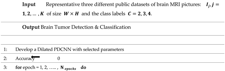
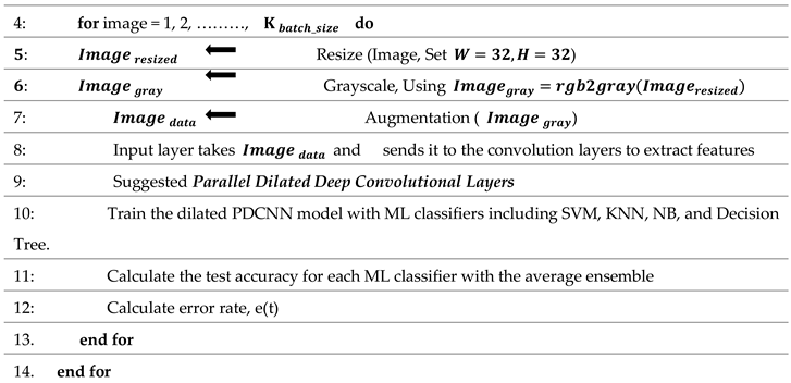
The step-by-step flow of the suggested framework is mentioned in Algorithm 1.
| Algorithm 1 Algorithm Based on Brain Tumor Detection and Classification Approach |
|
3.1. Dataset
This study makes use of three distinct public datasets containing images from brain MRIs. The details regarding the dataset are provided as follows.
Dataset-Ⅰ: Through the Kaggle platform, the initial accessible dataset of binary-class MRI scans of the brain has been obtained for simplicity and this dataset is widely used. This data is known as dataset-I in this study [8]. This set of 253 brain MRI images includes 98 samples with tumors and 155 samples without tumors.
Dataset-Ⅱ: The Figshare dataset containing 233 patients' brain MRI images is employed in this research [13]. These brain MRI images are obtained at Nanfang Hospital and General Hospital, two Chinese medical centers. This dataset, designated dataset-II, comprises 3064 brain MRI scans, including 1426 glioma tumors, 708 meningioma tumors, and 930 pituitary tumors.
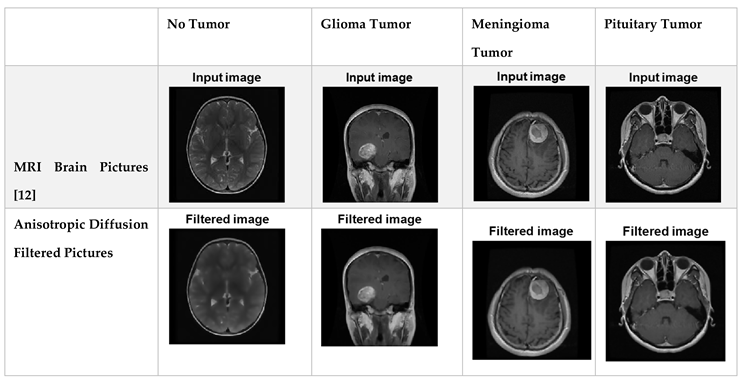
Dataset-Ⅲ: The additional dataset utilized in this study can also be obtained via the Kaggle website [14]; it contains brain MRI images of glioma tumor, meningioma tumor, no tumor, and pituitary tumor, numbered 826, 822, 395, and 827, in that order. This collection of data is identified as dataset-Ⅲ in the current research. The four different kinds of brain MRI images that are present in dataset-Ⅲ are shown in Figure 3.
3.2. Data Preprocessing
A method for enhancing the efficiency of a machine learning model is called data preprocessing, which involves purifying and preparing data for usage by the model. The skull photos in the MRI datasets are not all identical in width, and height; instead, each image is scaled to 32 x 32 pixels for training purposes. Grayscale conversion of these data contributes to a reduction in the level of complexity. Digital images can be noise-free without having their edges blurred through the utilization of the anisotropic diffusion filter.

Table 1.
Filtered Dataset after Utilization of Anisotropic Diffusion Filter.
3.3. Data Augmentation
Since deep learning needs a lot of data to extract information, data enhancement is being employed at this time to increase the quantity of available data by altering the initial image. Supplementary data can be used to increase the effectiveness of categorized outcomes. Illustrations can undergo the following procedures: shifting, scaling, translation, and filtering methods. This article uses the process of anisotropic diffusion filtering as augmentation.
Table 2.
Dataset Statistics.
| Category | Original Data | Augmented Data | ||||
| Number | Percentage | Number | Percentage | |||
| Dataset Ⅰ | Tumor | Yes | 98 | 61% | 196 | 61% |
| No | 155 | 39% | 310 | 39% | ||
| Total | 253 | 100% | 506 | 100% | ||
| Dataset Ⅱ | Glioma | 1426 | 47% | 2852 | 47% | |
| Meningioma | 708 | 23% | 1416 | 23% | ||
| Pituitary | 930 | 30% | 1860 | 30% | ||
| Total | 3064 | 100% | 6128 | 100% | ||
| Dataset Ⅲ | Glioma | 826 | 28.78% | 1652 | 28.78% | |
| Meningioma | 822 | 28.64% | 1644 | 28.64% | ||
| Pituitary | 395 | 13.76% | 790 | 13.76% | ||
| No Tumor | 827 | 28.81% | 1654 | 28.81% | ||
| Total | 2870 | 100% | 5740 | 100% | ||
3.4. Developed Dilated PDCNN Design
This paper presents the design of a multiscale dilated two simultaneous deep CNN technique to extract multiscale detail characteristics from MRI images. To increase the receptive field despite adding more parameters to the network, dilated convolution is used. Additionally, batch normalization is used to guarantee that the model's precision won't drop as the network depth increases.
The multiscale extraction of characteristics, integrating path, and classification stage are the three main elements of the suggested network, as illustrated in Figure 4. Since the suggested model uses dilated CNNs, the DF is an additional hyper-parameter that must be considered.
Both local and global characteristics are acquired in the dilated PDCNN framework through the corresponding local and global routes. However, most DCNN-based methods cannot effectively collect both local and global data because of their tiny receptive fields. Stacking multiple dilated convolutions has the disadvantage of creating a grid effect, even though dilated convolution maintains data resolution at the output layer and expands the receptive field without incorporating computation. In the event that, with poor DF, the model may contain a smaller receptive field nevertheless misses the coarse features. In contrast, with the excessive DF, the model is unable to pick up from the finer details. By contrasting various DFs, these suitable DFs are chosen for both local and global feature paths. Each of the convolutional layers is followed by the max-pooling layer for every single path that down samples the outcome of the convolutional layer and uses the ReLU activation function. In the end, an average ensemble method is employed to carry out the brain tumor categorization process after four ML classifiers—have been training the images.
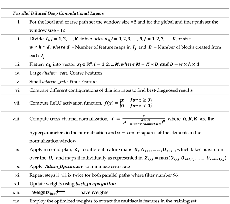
The step-by-step flow of the suggested dilated PDCNN structure is mentioned in Algorithm 2.
| Algorithm 2 Algorithm Based on Dilated PDCNN Model |
 |
3.4.1. Multiscale Feature Selection Path
CNNs have been used extensively in the field of medicine and have demonstrated good results in the segmentation and classification of medical images [22, 23]. CNN architectures are built using a variety of building blocks, such as Fully-Connected (FC) layers, Pooling layers, and Convolution layers. Convolution layers, which combine linear and nonlinear operations—that is, activation functions and convolution operations—are used in feature extraction [24,25]. Kernels and their hyperparameters, such as the size, quantity, stride, padding, and activation function of each kernel, are the parameters of convolution layers [26]. Six convolution layers are used in the two simultaneous paths and the convolution operation occurs using equation (1).
Where for kernel in layer expresses the resultant feature map of position, represents the weight vector’s values indicates the input vector of position in the and is the symbol of bias In addition, the activation function is [27]. By down-sampling, pooling layers lower the dimensionality of the feature maps. The stride, padding, and filter size are among the hyperparameters that comprise pooling layers, although they do not contain any other parameters. Two common varieties of pooling layers are max pooling and global average pooling. Maximum pooling layer is used in this structure. The output size of the pooling operation in CNN is calculated using equation (2).
where stands for the dimension of input, is the kernel size, the padding size is shown by , and is symbol of stride size [27].
The pooling layers' feature maps are smoothed out and sent to several one-dimensional (1D) vectors known as FC layers. The most popular activation parameter for FC layers is the Rectified Linear Unit (ReLU), which is illustrated in (3).
The final FC layer's activation function is usually SoftMax for the categorization of multiple classes and Sigmoid for binary classification. The node values in the final FC layer of the proposed model has computed using (4), and the sigmoid activation function for a binary categorization dataset-Ⅰ is calculated using (5) [24].
where stands for the neural network layers' internal calculations, shows the bias, and stands for the weights used to determine an output node's value. Furthermore, the input vector and output class are denoted by and , respectively. The SoftMax activation function is calculated using (6) for the multi-class categorization Figshare dataset-Ⅱ and Kaggle dataset-Ⅲ in this proposed structure.
where, stands for the input vector and for the class in the case of a multi-class categorization problem. Additionally, the component of the class rating vector in the final FC layer is displayed by . The category with the highest coefficient is chosen as the output class in the SoftMax activation function [24]. A backpropagation algorithm has used during CNN training to adjust the weights of the FC and convolution layers. The two main elements of backpropagation are the loss function and Gradient Descent (GD), in which GD is used to minimize the loss function. Among the loss functions most frequently employed by CNNs is the Cross-Entropy (CE) loss function. For the binary categorization dataset-Ⅰ with sigmoid activation function the CE loss function is computed using (7).
where computed using formula (4). For the multi-class categorization Figshare dataset-Ⅱ and Kaggle dataset-Ⅲ with the SoftMax activation function the CE loss function is calculated using (8) [27,28].
where denotes the quantity of training elements, input image class is indicated by , and the component of the category scores vector in the final FC layer is presented by [27].
Expanding the receptive field in deep learning involves boosting the dimension and depth of the convolution kernel, which in turn enhances the number of elements in the network. By adding weights of zero to the conventional convolution kernel, dilated convolution may enhance the receptive field without adding more network elements.
Equation (9) defines the convolution function * as follows: 1-D dilated convolution using DF, connects input image alongside kernel . The term "standard CNN" refers to this 1-D convolution. The network is identified as dilated CNN when rises.
Upon the introduction of a DF denoted as and through its expansion, is referred to as,
Using equation (10), the dilated convolution operation is calculated in this proposed structure. The fundamental CNN has a value of [28,29].
The main function of dilated convolution layer is to extract features. In addition to conveying fine and high-level feature details, MRI images also contain rough and low-level information. As a result, image data must be extracted at several scales. Specifically, the local and global routes are employed to obtain the local and global features. Within the local route, the convolutional layers make use of the small 5x5 pixel window dimension to provide low-level details about the images. However, a vast number of filters with 12x12 pixels are present in the convolutional stages of the global path. The same 5 by 5 filters are used by three different convolution layers throughout the local path, and each layer's decremental even number of high DF (4,2,1) is the only factor used to produce the coarse feature maps. Three distinct convolution layers in the global path employ identical 12 × 12 filters, and the generation of finer feature maps is exclusively dependent on the tiny DF (2,1,1) of every single layer. As illustrated in Figure 4, three convolution layers with distinct filter numbers (128, 96, 96) are applied at each feature extraction path to extract image data at various scales.
Conv1, Conv3, and Conv4 provide local as well as coarse features, while Conv2, Conv5, and Conv6 supply global as well as fine features. The max-pooling layer is employed after each convolutional layer for each path that down-samples the output of the convolutional layer. By employing a 2 × 2 kernel, the max-pooling layers lower the dimension of the attributes that are produced.
A dimension of (32, 32, 1) is assigned to each input tensor in the suggested model's structure. To test the impact of the DF on the model's efficiency and comprehend the gridding impact brought about by the dilation approach, the interior design is kept as simple as possible. In the local path, layer Conv1 applies a 5 × 5 filter and a dilation factor of =4 to generate coarse feature maps (such as shapes and contours); layer Conv3 applies the same filter and dilation factor of =2 along with the final convolution to generate coarse feature maps once more; and layer Conv4 applies a 5 × 5 filter and dilation factor of =1 to generate coarse feature maps. In the global route, layer Conv2 applies a 12 × 12 filter and a dilation factor of =2, layer Conv5 applies the same filter and dilation factor of =1 along with the last convolution to generate fine feature maps once more, and layer Conv6 applies a 12 × 12 filter and a dilation factor of =1 to generate fine feature maps. The activation function of ReLU is utilized by all six convolutional stages.
3.4.2. Merge Stage
A merge layer connects the two routes, creating a single path with a cascaded link until it reaches the endpoint. This process extracts multiscale features, where local paths with high dilation rates extract local as well as coarse features, and global paths with low dilation rates extract global as well as fine features. Two fully interconnected layers that are connected to a dropout layer through the merging pathway come after a batch normalization layer and a ReLU layer. In order to address the issue of performance degradation brought on by a boost in neural network stages, batch normalization is used. Equation (11) provides the feature map that results after a merging phase [19].
where σ stands for the ReLU activation function, BN denotes the batch normalization function and denotes the fused feature maps from each channel in the preceding paths.
3.4.3. Hyperparameter Tuning
Hyperparameter adjusting is a successful parameter searching technique for the suggested dilated PDCNN framework. The dense layer, optimization, and dropout measure are among the parameters that must be chosen to perform this PDCNN adjustment. It provides the framework with the ideal set of parameters, producing the most effective results.
The training data for the simulated scenario is provided by the effective adjustment of the hyperparameter, which includes the Adaptive Moment Estimation (Adam) optimizer, 0.3 dropout, 512 dense layers, and 0.0001 rate of learning. In this work, the weight of the layers is updated via Adam, the optimizer that calculates the adaptive learning rates of every parameter. The training setting employs a validation frequency of 20 Hz. The highest average accuracy for the test datasets is collected for each run. When the epoch count reaches 70, the framework is trained employing a range of epoch counts; it acquires 98.67% accuracy for dataset-Ⅰ. It acquires 98.13% and 98.35% accuracy for dataset-Ⅱ, and dataset-Ⅲ respectively when the epoch number is 60.
Table 3.
Hyper-parameter Settings for Model Training.
| Hyper-Parameter | Optimized Value |
| Optimizer | Adam |
| Dropout | 0.3 |
| Dense Layer | 512 |
| Learning Rate | 0.0001 |
| Maximum Epoch | 50 |
| Validation Frequency | 20 |
| Iteration Per Epoch | 34 |
3.4.4. Feature Map of Dilated Convolutional Layers
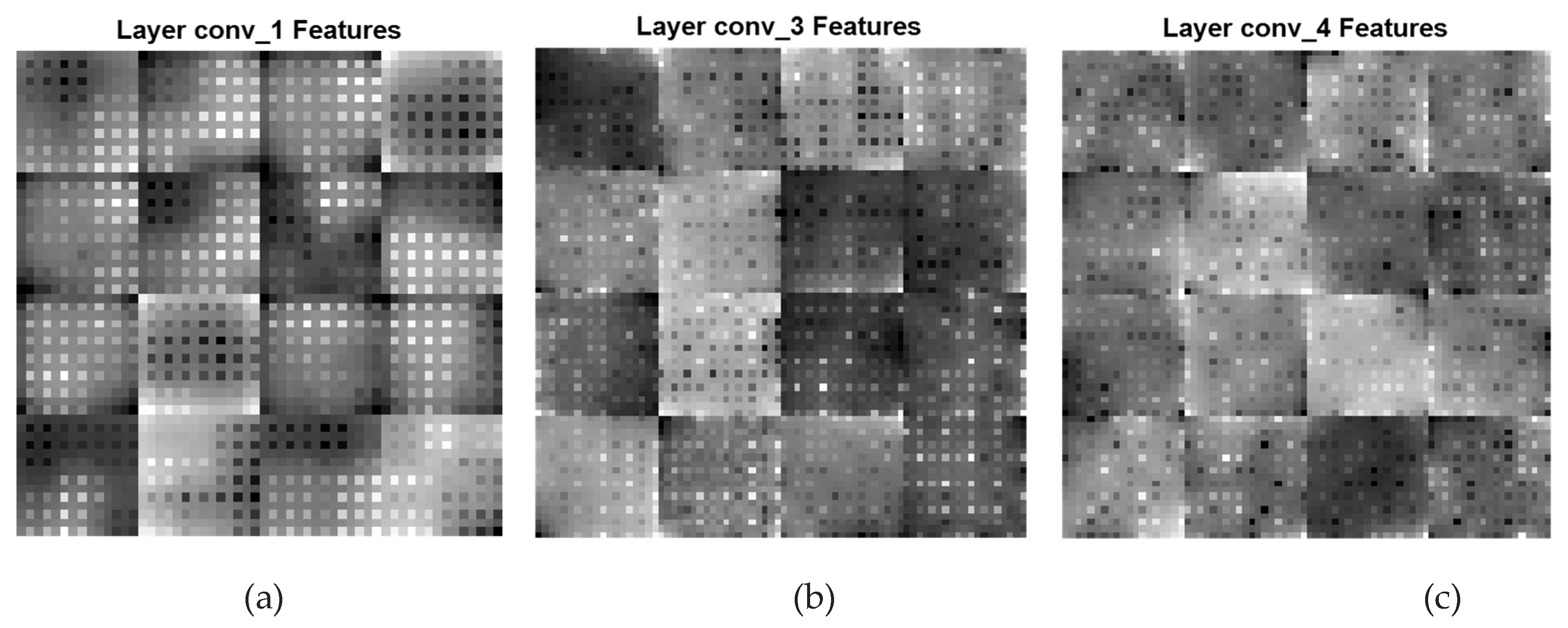
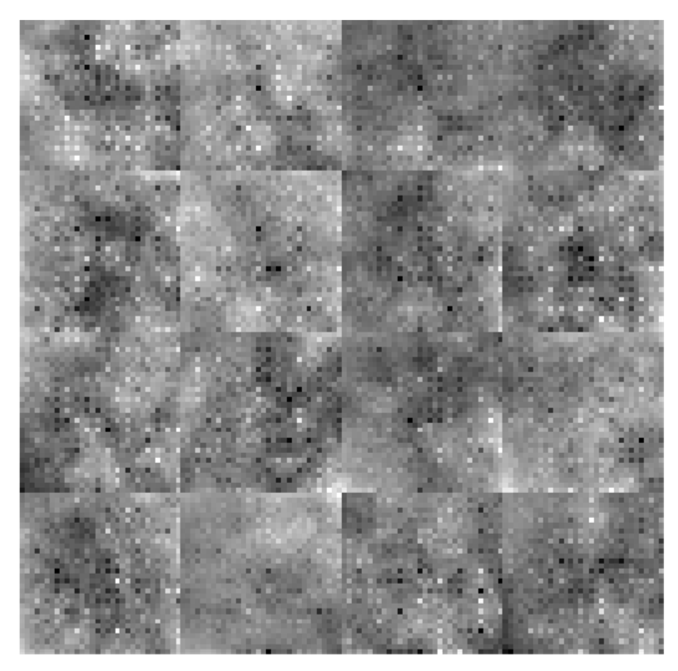
A CNN feature map represents specific attributes in the input image as the result of a convolutional layer. It is produced by filtering input images or the previous layers' feature map output. The feature maps that are acquired from every convolutional layer are presented in Figure 5 and Figure 6. In Figure 5, the low-level and coarse features of the three convolutional layers conv_1, conv_3, and conv_4 having filters of 128, 96, and 96 are displayed. The feature maps in this figure are primarily composed of coarse and local features which represent the texture in an image. In this local path, a dilated CNN algorithm that has DFs associated with (= 4, = 2, = 1) is referred to as dilated PDCNN (4, 2, 1). In Figure6, the high-level feature maps include contour representations, shape descriptors and fine features of the deeper three convolutional layers conv_2, conv_5, and conv_6 having the same filters, are shown. DFs corresponding to (=2,= 1, = 1) are used in this global path. The multiscale feature maps, which are displayed in Figure 7, are greatly improved when these features are combined using a feature fusion technique. Figure 8 displays the final multiscale features that are extracted, along with a fully connected layer that is prevented from overfitting by employing the dropout technique.
Local & Coarse Features (conv_1[DF:4*4], conv_3[DF:2*2], and conv_4[DF:1*1])
Figure 5.
Local and Coarse feature maps of various convolutional layers of the Dilated PDCNN (a) Feature map of conv_1-layer (b) Feature map of conv_3-layer (c) Feature map of conv_4-layer.
Figure 5.
Local and Coarse feature maps of various convolutional layers of the Dilated PDCNN (a) Feature map of conv_1-layer (b) Feature map of conv_3-layer (c) Feature map of conv_4-layer.
Global & Finer Features (conv_2[DF:2*2], conv_5[DF:1*1], and conv_6[DF:1*1])
Figure 6.
Global and finer feature maps of various convolutional layers of the Dilated PDCNN (a) Feature map of conv_2-layer (b) Feature map of conv_5-layer (c) Feature map of conv_6-layer.
Figure 6.
Global and finer feature maps of various convolutional layers of the Dilated PDCNN (a) Feature map of conv_2-layer (b) Feature map of conv_5-layer (c) Feature map of conv_6-layer.
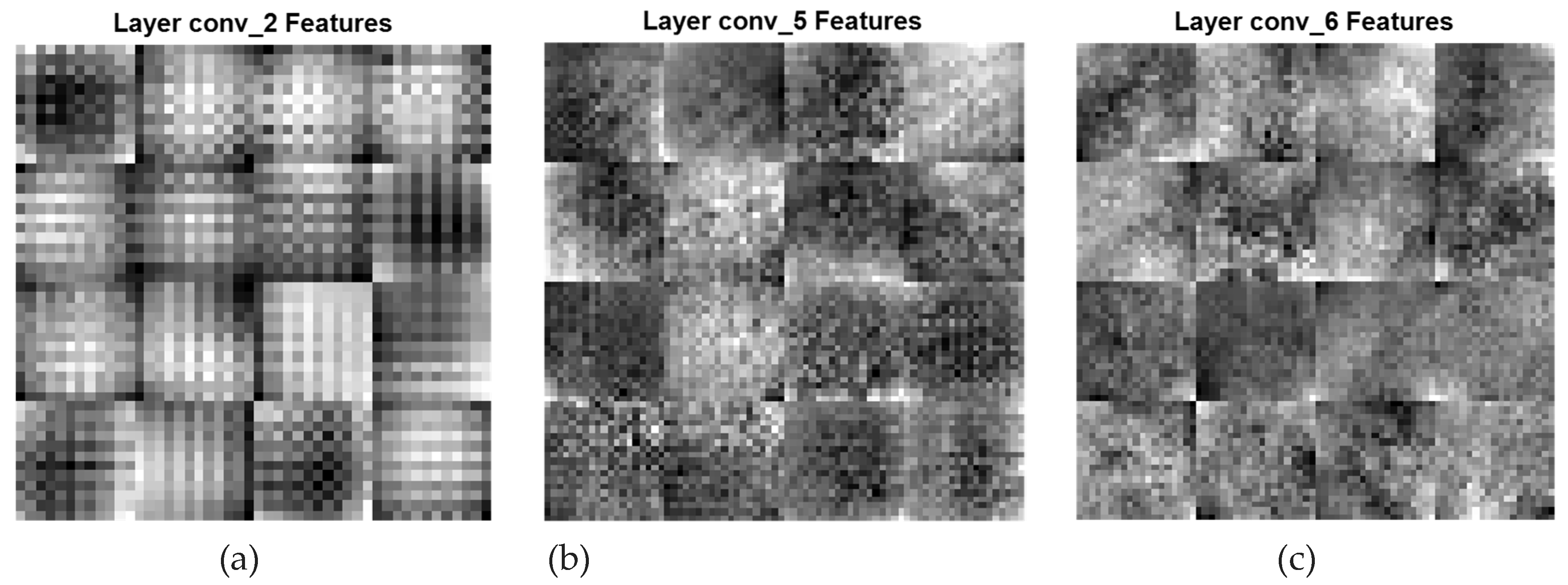
Figure 7.
Addition of all features.
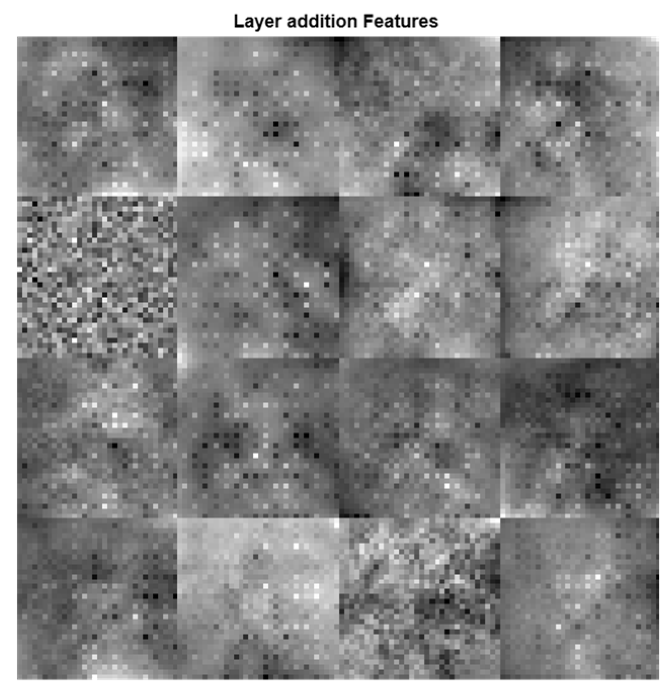
Figure 8.
Features extraction after FC_2 layer.
3.4.5. Parameters for Dilated PDCNN Model
Both FC and convolutional layers provide parameters that can be learned. Parameters are the quantities of weights that the CNN structure learns during training. It is possible to calculate the convolutional layer parameters () equation as follows:
and stand for the length and width of the filter, accordingly. indicates the quantity of filters. indicates the associated layer's input channel quantity. The parameters of the layer that is fully connected () are as follows:
where indicates the prior layer's activation pattern and denotes the number of neurons that make up the present FC layer. There are no variables that can be learned in the max-pooling layer. The batch-normalization layer's variables are the product of the number of channels utilized in the preceding convolutional layer [10].
Table 4.
Information about the Suggested Dilated PDCNN Framework.
| Layer Type | No of Filters | Filter Size | Stride | Dilation Factor | Activation Shape | Total Learnable Parameters |
|---|---|---|---|---|---|---|
| Image MRI | - | - | - | - | 32×32×1 | 0 |
| Conv layer | 128 | 5×5 | 2,2 | 4,4 | 16×16×128 | 3328 |
| ReLU | - | - | - | - | 16×16×128 | 0 |
| Cross Channel Normalization | - | - | - | - | 16×16×128 | 0 |
| Max Pooling | - | 2×2 | 2,2 | - | 8×8×128 | 0 |
| Conv layer | 96 | 5×5 | 2,2 | 2,2 | 4×4×96 | 307296 |
| Conv layer | 128 | 12×12 | 2,2 | 2,2 | 16×16×128 | 18560 |
| ReLU | - | - | - | - | 4×4×96 | 0 |
| Max Pooling | - | 2×2 | 2,2 | - | 2×2×96 | 0 |
| Conv layer | 96 | 5×5 | 2,2 | 1,1 | 1×1×96 | 230496 |
| ReLU | - | - | - | - | 1×1×96 | 0 |
| Max Pooling | - | 2×2 | 2,2 | - | 1×1×96 | 0 |
| ReLU | - | - | - | - | 16×16×128 | 0 |
| Cross-Channel Normalization | - | - | - | - | 16×16×128 | 0 |
| Max Pooling | - | 2×2 | 2,2 | - | 8×8×128 | 0 |
| Conv layer | 96 | 12×12 | 2,2 | 1,1 | 4×4×96 | 1769568 |
| ReLU | - | - | - | - | 4×4×96 | 0 |
| Max | - | 2×2 | 2,2 | - | 2×2×96 | 0 |
| Conv layer | 96 | 12×12 | 2,2 | 1,1 | 1×1×96 | 1327200 |
| ReLU | - | - | - | - | 1×1×96 | 0 |
| Max Pooling | - | 2×2 | 2,2 | - | 1×1×96 | 0 |
| Elements-wise addition of 2 inputs | - | - | - | - | 1×1×96 | 0 |
| Batch Normalization | - | - | - | - | 1×1×96 | 192 |
| ReLU | - | - | - | - | 1×1×96 | 0 |
| FC_1 layer | - | - | - | - | 1×1×512 | 49664 |
| ReLU | - | - | - | - | 1×1×512 | 0 |
| Dropout layer | - | - | - | - | 1×1×512 | 0 |
| FC_2 layer | - | - | - | - | 1×1×2 | 1026 |
| Total = 3, 707, 330 |
3.5. Classification Stage
In this categorization phase, extracting all the multiscale attributes from the last FC layer, four types of classifiers: SVM, KNN, NB, and Decision tree are used to categorize the three types of brain tumor datasets. These ML classifiers and their hyper-parameter settings used in this experiment for brain tumor classification are discussed in the following subsections.
3.5.1. SVM
SVM, proposed by Vapnik, is one of the most powerful classification algorithms that works by creating a hyperplane with the maximum margin between classes. SVM uses the kernel function,, to transform the original data space into another space with a higher dimension. The hyperplane function for separating the data can be defined as follows [30]:
where is support vector data (deep features from brain MR image), is Lagrange multiplier, and represent a target class of these three datasets employed in this paper, such that the first dataset is binary (normal and abnormal) class dataset, while the second dataset has three classes (glioma, meningioma, and pituitary) and the third dataset has four different classes (normal, glioma, meningioma, and pituitary tumor) with n = 1, 2, 3, ..., N. In this work, the most commonly used kernel function is used at the SVM algorithm is linear kernel.
As shown in (15), an actually separable case is handled using a linear kernel.
where represents kernel function.
Hence, a multiclass linear support vector machine with a linear kernel function and a zero verbose value is employed in this suggested method.
3.5.2. K-NN
k-NN is one of the simplest classification techniques. It performs predictions directly from the training set that is stored in the memory. For instance, to classify a new data instance (a deep feature from brain MR image), k-NN chooses the set of k objects from the training instances that are closest to the new data instance by calculating the distance and assigns the label with two classes (normal or tumor), three classes (glioma, meningioma, and pituitary) or four classes (normal, glioma, meningioma, and pituitary tumor) and does the selection based on the majority vote of its k neighbors to the new data instance.
Manhattan distance and Euclidean distance are the most commonly used to measure the closeness of the new data instance with the training data instances. In this work, the Euclidean distance is used to measure for the k-NN algorithm. Euclidean distance between data point and data point are calculated as follows [27]:
The brief summary of k-NN algorithm is illustrated below:
- ▪
- First select a suitable distance metric.
- ▪
- Store all the training data set in pairs in the training phase as follows:where in the training dataset, is a training pattern, is the amount of training patterns and is its corresponding class.
- ▪
- In the testing phase, compute the distances between the new features vector and the stored (training data) features, and classify the new class example by a majority vote of its k neighbors.
The correct classification given in the test phase is used to evaluate the accuracy of the algorithm. If the result is not satisfactory, the k value can be adjusted until a reasonable level of accuracy is obtained. It is noticeable here that the number of neighbors is set from 1 to 5 and selected the optimum value of K is 5 which is applied for dataset-Ⅰ, dataset-Ⅱ, and dataset-Ⅲ respectively with the highest accuracy. The zero standardized value is used to standardize the predictors.
3.5.3. Naïve Bayes (NB)
NB classifier is the ML classifier with the assumption of conditional independence between the attributes given the class. In this article, the final class is predicted using vectors of attributes and class prior probabilities, as shown in (18).
Where indicates the given data instance (extracted deep features from brain MR image) which is represented by its feature vector () and is the class target (type of brain tumor) with two classes (normal and tumor) for binary dataset-Ⅰ or three classes (glioma, meningioma, and pituitary) for Figshare dataset-Ⅱ, or four classes (normal, glioma, meningioma, and pituitary) for multiclass Kaggle dataset-Ⅲ . Here, in this classifier is computed by taking the dataset's features to be independent, and calculating the probability as shown in (19) [27].
NB can save a significant amount of time and is appropriate for handling multi-class prediction problems. The value for the minimum threshold of probabilities for the NB classifier is 0.001. For every predictor and class combination, the kernel smoothing window width is automatically chosen by default in this suggested approach.
3.5.4. Decision Tree
For both classification and regression, decision tree structures are a non-parametric supervised learning technique. In this work, this technique is employed to build a model that, by utilizing basic decision rules deduced from the data features extracted from brain MR images. With training vectors , i= 1,…,l and a label vector , a decision tree successively divides the domain of features so that instances that share similar desired values are organized together [31].
Three datasets are used in this proposed approach. Here dataset-Ⅰ at node be denoted by . Splitting for every candidate which is composed of a characteristic j and threshold ,dividing the dataset-Ⅰ, into and subgroups
Next, to calculate the quality of a potential split of node m, a loss function H() is used.
This process should be carried out for and subsets until the maximum permitted depth is achieved. These steps are also followed for the other two datasets multiclass Figshare dataset-Ⅱ and Kaggle dataset-Ⅲ.
The decision tree can quickly determine which data is relevant and which is not. The maximum number of branch nodes in the suggested method is fixed at 1. In this approach, there must be a minimum of one leaf node.
3.5.5. Average Ensemble Method
Machine learning and signal analysis both use the statistical technique of ensemble averaging. Model averaging is a machine learning technique for ensemble learning in which each member of the ensemble makes an equal contribution to the ultimate prediction. A group of frameworks often outperforms a single one because the individual errors in the models "average out." In average ensemble method, the actions are:
- ⮚
- Create N experts, each starting at a different value: Typically, initial values are selected at random from a distribution.
- ⮚
- Train every specialist independently.
- ⮚
- Add up all the experts and take the mean of their scores.
4. Experimental Outcomes and Evaluation
MATLAB is used to run the implementation program for the suggested dilated PDCNN model. The computing device is equipped with a Core i5 processor manufactured by Intel, running at 3.2 GHz, eight GB of RAM, and Windows 10 operating system installed.
4.1. Performance Analysis of Suggested Dilated PDCNN Model
The confusion matrix is used to express the classification system's results. The efficiency is evaluated using the following criterion [34].
Table 5 provides an overview of the dilated PDCNN algorithm's efficiency indicators using ML classifiers over dataset-Ⅰ. As per Table 5 findings, the dilated PDCNN model that incorporates KNN and Decision Tree classifiers has the best F1-score, recall, accuracy, and precision in comparison with the remaining models. The suggested dilated PDCNN model utilizing KNN and Decision Tree classifiers has 100.00% for all performance criteria, which is better than the outcomes obtained by other ML classifiers. The dilated PDCNN model that includes SVM and NB classifiers is noteworthy for having 100% precision and recall, which is also the same as the dilated PDCNN model alongside KNN and Decision Tree classifiers. However, the KNN and Decision Tree classifier execute better concerning other performance indicators. The suggested dilated PDCNN utilizing the average ensemble approach for the dataset-Ⅰ has finalized accuracy, precision, recall, and F1-score values of 98.67%, 98.62%, 99.17%, and 98.28%, accordingly, after implementing the average ensemble technique.
An overview of the dilated PDCNN algorithm's efficiency indicators using ML classifiers over dataset-Ⅱ is provided in Table 6. The results shown in Table 6 demonstrate that, when contrasted to other scenarios, the dilated PDCNN algorithm using the NB classifier provides the highest performance indicators. The suggested dilated PDCNN model incorporating the NB classifier outperforms the findings of the remaining ML classifiers alongside accuracy of 98.90%, precision of 98.67%, recall of 98.67%, and F1-score of 98.67%. In the end, using the average ensemble approach, the suggested dilated PDCNN employing the average ensemble technique for the dataset-Ⅱ has accuracy, precision, recall, and f1-score values of 98.13%, 97.74%, 98.05%, and 97.80%, accordingly.
Table 7 provides an overview of the effective measurements of the suggested dilated PDCNN model using machine learning classifiers for dataset-Ⅲ. In comparison to other models, the accuracy, precision, recall, and F1-score of the suggested dilated PDCNN alongside SVM classifier are 98.60%, 98.50%, 98.25%, and 98.50%, respectively, based on the results shown in Table 7. The findings of the dilated PDCNN employing average ensemble technique for dataset-Ⅲ are, after executing the average ensemble strategy, 98.35%, 98.35%, 97.85%, and 98.20%, accordingly, in terms of accuracy, precision, recall, and F1-score.
4.2. Comparative Analysis of Different Dilation Rate
While dilated convolution retains data resolution at the output layer and increases the receptive field without adding computation, stacking several dilated convolutions has the drawback of producing a grid effect. Validating the results involves comparing multiple combinations of dilation rates for the various convolution layers. Large dilation rates may impact tiny object recognition. As a result, the DF has gradually decreased (even-numbered arithmetic decreasing) at the local path in the suggested framework. By doing this, the dilated feature map's sparsity is reduced, and more data can be extracted from the investigated region. At the global path, the low DF (2,1,1) has been carried out to extract the fine features.
A comprehensive review of the gridding issue and the consequences of different dilation rates can be found in the accompanying Figure 9. The poor efficiency of the (4, 2, 1) dilated value for the global pathway as well as (8, 4, 2) dilated value for the local route of the suggested model is caused by the gridding phenomenon, which arises when high DF are used. This limits the framework from acquiring finer characteristics. When a high DF (4,2,1) is used for both local and global paths, the accuracy increases more than before. On the contrary, using low dilation rates, the model only learns fine features. When low DF (1,1,1) is used in the global path and (2,2,2) is used for the local path, the value of accuracy for dataset-Ⅰ, dataset-Ⅱ, and dataset-Ⅲ is 97.30%, 97.70%, and 93.70% respectively. When a low DF (2,1,1) is used for the global feature and a high DF (4,2,1) is used for the local feature, the highest accuracy is achieved. The highest accuracy for dataset-Ⅰ, dataset-Ⅱ, and dataset-Ⅲ is 97.33%, 98.20%, and 97.94% respectively. Providing the best-case scenario, a well-balanced model (4,2,1) for the local path and (2,1,1) for the global path may acquire both the coarse as well as fine characteristics of the pictures.
4.3. Evaluation Measurements of the Proposed System on the Three Datasets
With the SVM, KNN, NB, and Decision Tree classifiers for dataset-Ⅰ, Table 8 illustrates the classification accuracy, erroneous, duration, and kappa scores for the suggested PDCNN as well as dilated PDCNN architectures. When the expected precision of the random classifier is considered, the kappa statistic expresses how closely the instances identified by the classification model matched the data assigned as ground truth. In comparison to the PDCNN alongside the average ensemble model, the dilated PDCNN has a larger kappa. The error rate has reduced, and the elapsed time has increased following the application of dilation to the PDCNN with the average ensemble model.
The success rate, error, period, and kappa statistics for the suggested PDCNN and dilated PDCNN architectures employing the SVM, KNN, NB, and Decision Tree classifiers for dataset-Ⅱ are presented in Table 9. When the expected precision of the random classifier is considered, the kappa statistic expresses how closely the instances identified by the classification model matched the data assigned as ground truth. As compared to the PDCNN employing the average ensemble model's kappa, the dilated PDCNN offers greater kappa. The error rate has dropped when dilation is applied to the PDCNN using the average ensemble method, but the time that passed has increased.
Table 10 presents the kappa values, accuracy, error, and training duration for the recommended PDCNN and dilated PDCNN models that employ the SVM, KNN, NB, and Decision Tree classifiers for dataset-Ⅲ, in that order. When compared to the PDCNN employing an average ensemble model, the dilated PDCNN has a higher kappa value. The error rate has reduced, and the elapsed time has increased following the application of dilation to the PDCNN with the average ensemble model.
4.4. Impact of Applying Dilation on the Proposed Model
In the categories of efficiency, precision, recall, F1-score, error rate, kappa, and training time, Figure 10 shows that the suggested dilated PDCNN alongside the average ensemble approach executes better than the conventional PDCNN alongside the average ensemble framework. Values of the effectiveness indicators will increase even further if dilation is applied to increase the efficiency of the recommended approach.
These findings show that in comparison to the proposed PDCNN model using the average ensemble technique, the proposed dilated average ensemble classifier for three types of dataset indicates a higher accuracy, precision, recall, F1-score, kappa, and lower error rate, execution time.
4.5. Comparison of the Suggested Model with Prior Investigations Based on Three Datasets
A comprehensive assessment is made at the end of the validation process for the proposed approach. A brief overview is shown in Table 11.
5. Discussion
With an increasing number of patients, manually analyzing MRI images has grown more complicated, time-consuming, and frequently inaccurate. Conventional machine learning techniques utilize handmade properties, which reduces the solution's durability and raises its cost. Nonetheless, there are situations when supervised learning models perform better than unsupervised learning strategies, leading to an overfitted structure that is inappropriate for another large database. These problems emphasize how crucial it is to create a fully machine learning-based classification system for brain tumors. By combining the average ensemble technique with PDCNN, this investigation presents a novel approach to the identification and classification of brain tumors. The dilated PDCNN architecture includes both local and global multiscale feature selection paths, a merging phase, and categorization pathways. The initial pictures are converted to grayscale, which makes the process easier. After that, new images are made from old ones by employing data augmentation. Using a modest window size of 5x5 pixels and gradually high dilation rates (4,2,1) for each convolution layer, the convolutional layers in the local path collect coarse characteristics and provide local data to the images. In contrast, the global path's convolutional layers obtain fine details by using a large window dimension of 12 by 12 pixels and low dilation rates (2,1,1) for every layer of convolution. ReLU activation function and max-pooling layer are applied after each convolutional layer for each path that down-samples the convolutional layer output. A fusion layer connects the two parallel pathways, forming a single path with a cascading link that continues until it reaches the end destination. Two fully connected layers that are attached to a dropout layer that is included in the merging route come after a batch-normalized layer and a ReLU layer. At the output path, the four classifier types—SVM, KNN, NB, and Decision Tree—are used to execute the brain tumor categorization procedure. A regularization method called dropout is also employed to stop the training data from being overfitting.
Table 5, Table 6 and Table 7 present the performance parameters of dilated PDCNN model with ML classifiers on binary Dataset-Ⅰ, multiclass figshare Dataset-Ⅱ and Multiclass Kaggle Dataset-Ⅲ. Among all the performance metrics, including accuracy, precision, recall, and F1-score, for three different brain tumor datasets employing the average ensemble technique, binary classification Dataset-Ⅰ provides the best outcomes. The value of accuracy, precision, recall, and F1-score of dilated PDCNN model on binary classification Dataset-Ⅰ is 98.67%, 98.62%, 99.17% and 98.28% respectively.
The impact of different dilation rates on the model's accuracy has been examined for the dilated PDCNN. The comparison analysis among various dilation rate arrangements for the various convolution layers is displayed in Figure 9. The comparative study demonstrates that the decremental large dilation rate (4, 2, 1) for the local path and the low dilation rate (1, 1, 1) for the global path yield the best results, based on an understanding of the gridding phenomenon and various recommendations for the dilation rate parameter for each layer. For datasets I, II, and III, the highest accuracy values obtained are 98.67%, 98.13%, and 98.35%. This demonstrates that while the global path (lower dilation rates) gains knowledge from the finer features, the local path (higher dilation rates) concentrates on the coarse features. The best outcomes are obtained with this combination.
Table 8, Table 9 and Table 10 displays the evaluation results including accuracy, error rate, time and kappa value of the proposed system on the three types of datasets. The lowest error rate 1.33% is provided by binary classification Dataset- I, and the highest value of kappa is provided by 0.977 is provided by multiclass Kaggle Dataset-Ⅲ.
The results shown in Figure 10 demonstrate that in terms of accuracy, precision, recall, F1-score, error rate, kappa, and training duration, the suggested dilated PDCNN with the average ensemble model performs better than the standard PDCNN with the average ensemble approach. The performance indicators' values will increase even further if the three different types of datasets are dilated to increase the suggested dilated PDCNN's efficiency with the average ensemble model. A thorough comparison is done once the evaluation of the proposed method is accomplished. The findings demonstrate that the suggested simultaneous network topology outperforms detection and classification techniques that have been previously published.
6. Conclusion and Future Work
Since brain tumors vary in shape, dimension, and structure, proper identification of these conditions remains extremely difficult. It is well-known how important it is to detect brain tumors early to receive the right medical care. This study proposed a dilated PDCNN structure with ML classifiers to detect and classify brain tumors from MRI images. The proposed dilated PDCNN with the average ensemble method is evaluated for binary and multi-class classification on the Kaggle dataset, which contains four different types of tumor images, while the Figshare dataset contains three types of tumor images. The suggested dilated convolution with an expanded receptive field of the kernel has increased the computation efficiency while preserving high accuracy. The framework achieved outstanding accuracy, precision, recall, and F1-score regarding the binary brain cancer dataset-Ⅰ. In order to gain a better understanding of the inner workings of the network and its effectiveness of the dilation rate parameter, experimental evaluation can be performed on other datasets in future investigations. Additionally, studies can be carried out to identify brain tumors with greater accuracy by utilizing actual patient information from any source (various images captured by scanners).
Acknowledgement
This research is funded by Woosong University Academic Research 2024.
References
- T. A. Sadoon, M. H. A. Al-Hayani, “Deep Learning Model for Glioma, Meningioma and Pituitary Classification,” International Journal of Advances in Applied Sciences (IJAAS), vol. 10, no. 1, pp. 88–98, March 2021.
- M. Kheirollahi, S. Dashti, Z. Khalaj, F. Nazemroaia, P.Mahzouni, “Brain tumors: Special characters for research and banking,” Advanced Biomedical Research, 6 January 2015.
- R. Vankdothu, M. A. Hameed, “Brain Tumor MRI Images Identification and Classification Based on the Recurrent Convolutional Neural Network,” Measure: Sensors, 24, 28 September, 2022.
- [Online]. Available: “Quick Brain Tumor Facts |, Quick Brain Tumor Facts”, National Brain Tumor Society,2023.
- S. Irsheidat, R. Duwairi, “Brain Tumor Detection Using Artificial Convolutional Neural Networks,” 2020 11th International Conference on Information and Communication Systems (ICICS), 2020, pp. 197– 203.
- M. Toğaçar, B. Ergen, Z. Cömert, “BrainMRNet: Brain Tumor Detection using Magnetic Resonance Images with a Novel Convolutional Neural Network Model,” Medical Hypotheses, Volume 134, 1 January 2020.
- X. Jiang, Y. Jin, Y. Yao, “Low-dose CT lung images denoising based on multiscale parallel convolution neural network,” The Visual Computer, 37, pp.2419-2431, 2021.
- Brain MRI Images for Brain Tumor Detection | Kaggle.
- R. Yamashita, M. Nishio, R. K. G. Do, and K. Togashi, “Convolutional neural networks: an overview and application in radiology,” Insights into imaging, pp. 611-629, 2018.
- Z. A. Sejuti, M. S. Islam, “A hybrid CNN-KNN approach for identification of COVID-19 with 5-fold cross-validation,” Sensors International, Volume 4, p. 100229, 2023.
- L. Guimin, W. qingxiang, Q. Lida, H. Xixian, “Image Super-resolution Using a Dilated Convolutional Neural Network,” Neurocomputing, Volume 275, pp. 1219-1230, 31 January 2018.
- P. Afsar, K.N.Plataniotis, A. Mohammadi, “Capsule Networks for Brain Tumor Classification based on MRI Images and Coarse Tumor Boundaries,” In ICASSP 2019 IEEE International Conference on Acoustics, Speech and Signal Processing (ICASSP), Brighton, UK, pp. 1368-1372, 2019.
- Jun Cheng, 2017 Figshare dataset https://figshare.com/articles/brain tumor dataset/1512427.
- Brain Tumor MRI Dataset | Kaggle.
- Anil, A. Raj, H. A. Sarma, N. Chandran R, Deepa P L, “Brain Tumor detection from brain MRI using Deep Learning,” International Journal of Innovative Research in Applied Sciences and Engineering (IJIRASE), Volume 3, Issue 2, August 2019, pp. 68–73.
- Sajjad, M., Khan, S., Muhammad, K., Wu, W., Ullah, A. and Baik, S.W., 2019. Multi-grade brain tumor classification using deep CNN with extensive data augmentation. Journal of computational science, 30, pp.174-182.
- Brain Tumor Detection Using Convolutional Neural Networks | by Mohamed Ali Habib | Medium 25 November 2021.
- F. J. Díaz-Pernas, M. Martínez-Zarzuela, D. González-Ortega, and M. Antón-Rodríguez, “A deep learning approach for brain tumor classification and segmentation using a multiscale convolutional neural network,” Healthc., vol. 9, no. 2, 2021. [CrossRef]
- M. K. Abd-Ellah,, A. I. Awad, H. F. A. Hamed, and A. A. M. Khalaf. "Parallel deep CNN structure for glioma detection and classification via brain MRI Images,” In 2019 31st International Conference on Microelectronics (ICM), pp. 304-307, 2019.
- K. Adu, Y. Yu, J. Cai, N. Tashi, “Dilated Capsule Network for Brain Tumor Type Classification Via MRI Segmented Tumor Region,” International Conference on Robotics and Biomimetics Dali, China, pp.942-947, December 2019. [CrossRef]
- A.E. Minarno, M. H. C. Mandiri, Y.Munarko, Hariyady, “Convolutional Neural Network with Hyperparameter Tuning for Brain Tumor Classification," Kinetik: Game Technology, Information System, Computer Network, Computing, Electronics, and Control,vol.6, no.2, pp.127-132, May 2021.
- R. Yamashita, M. Nishio, R. K. G. Do, K. Togashi, “Convolutional neural networks: An overview and application in radiology,” Insights Imag., vol. 9, pp. 611–629, Aug. 2018. [CrossRef]
- C. Zhou, J. Song, S. Zhou, Z. Zhang, J. Xing, “COVID-19 detection based on image regrouping and resnet-SVM using chest X-ray images,” IEEE Access, vol. 9, pp. 81902–81912, 2021. [CrossRef]
- S. Y. Sourab, M. A. Kabir, “A comparison of hybrid deep learning models for pneumonia diagnosis from chest radiograms,” Sensors International, Volume 3, pp. 100167, 2022.
- K. Balaji, K. Lavanya, “Medical image analysis with deep neural networks,” in Deep Learning and Parallel Computing Environment for Bioengineering Systems, pp. 75–97, USA, 2019.
- E. Fathi, B. M. Shoja, “Deep neural networks for natural language processing,” in Handbook of Statistics, vol. 38, pp. 229–316, Elsevier, 2018.
- M. Yaseliani, A. Z. Hamadani, A. I. Maghsoodi, A. Mosavi, “Pneumonia Detection Proposing a Hybrid Deep Convolutional Neural Network Based on Two Parallel Visual Geometry Group Architectures and Machine Learning Classifiers,” IEEE Access, Volume 10, p.62110-62128, June 13, 2022.
- S. S. Roy, N. Rodrigues, Y-h. Taguchi, “Incremental Dilations Using CNN for Brain Tumor Classification,” Applied Sciences,2020. [CrossRef]
- N. Kesav, M.G. Jibukumar, “Efficient and low complex architecture for detection and classification of brain tumor using with two channel CNN,” Journal of King Saud University-Computer and Information Sciences, Volume 34, Issue 8, pp.6229-6242, September 2022.
- J. Cervantes, F. Garcia-Lamont, L. Rodríguez-Mazahua, and A. Lopez, “A comprehensive survey on support vector machine classification: Applications, challenges and trends,” Neurocomputing, vol. 408, pp. 189–215, Sep. 2020. [CrossRef]
- [Online]. 1.10. Decision Trees — scikit-learn 1.3.1 documentation last accessed on 24/10/2023.
- Dietterich, Thomas G, “Ensemble methods in machine learning,” International workshop on multiple classifier systems, pp.1-15, Berlin, Heidelberg: Springer Berlin Heidelberg, 2000.
- M. Bhuiyan, M.S. Islam, “A new ensemble learning approach to detect malaria from microscopic red blood cell images,” Sensors International, Volume 4, p. 100209, 2023.
- T. Rahman, M. S. Islam, “MRI brain tumor detection and classification using parallel deep convolutional neural networks,” Measurement: Sensors, Volume 26, p.100694, 2023.
- C.L. Choudhury, C. Mahanty, R. Kumar, “Brain tumor detection and classification using convolutional neural network and deep neural network,” 2020 International Conference on Computer Science, Engineering and Applications (ICCSEA), 2020, pp.1-4.
- H. H. Sultan, N. M. Salim, W. Al-Atabany, “Multi-Classification of Brain Tumor Images Using Deep Neural Network,” IEEE Access, May 27,2019, pp. 69215-69225.
- S. Priyansh, A. Maheshwari, S. Maheshwari, “Predictive Modeling of brain tumor: A Deep Learning Approach,” Innovations in Computational Intelligence and Computer Vision, Volume 3, Issue 2, 2021, pp. 275–285.
- T. Rahman, M. S. Islam, “MRI Brain Tumor Classification Using Deep Convolutional Neural Network,” 2022 3rd International Conference on Innovations in Science, Engineering and Technology (ICISET), 26-27 February 2022, Chittagong, Bangladesh.
- Biswas, M. S. Islam, “A Hybrid Deep CNN-SVM Approach for Brain Tumor Classification,” Journal of Information Systems Engineering and Business Intelligence, Volume 9, No.1, April 2023.
- H. A. Munira, M. S. Islam, “Hybrid Deep Learning Models for Multi-classification of Tumour from Brain MRI,” Journal of Information Systems Engineering and Business Intelligence, Volume 8, No.2, October 2022.
Figure 1.
MRI scans are performed on two different brains. On the left is a tumor, and on the right is a healthy [8].
Figure 1.
MRI scans are performed on two different brains. On the left is a tumor, and on the right is a healthy [8].
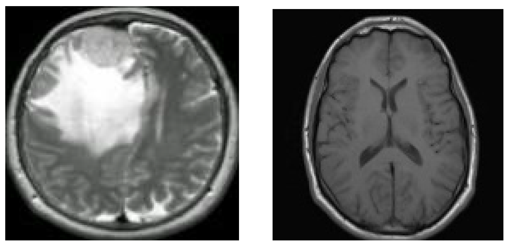
Figure 2.
Proposed methodology’s workflow.
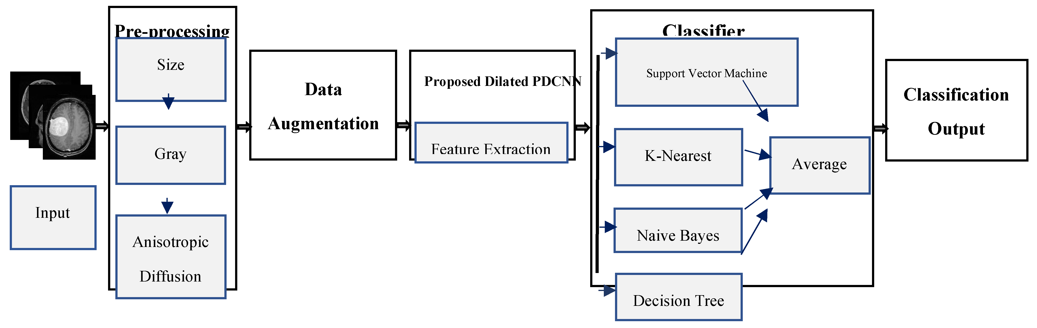
Figure 3.
Examples of brain MR images [14].
Figure 3.
Examples of brain MR images [14].
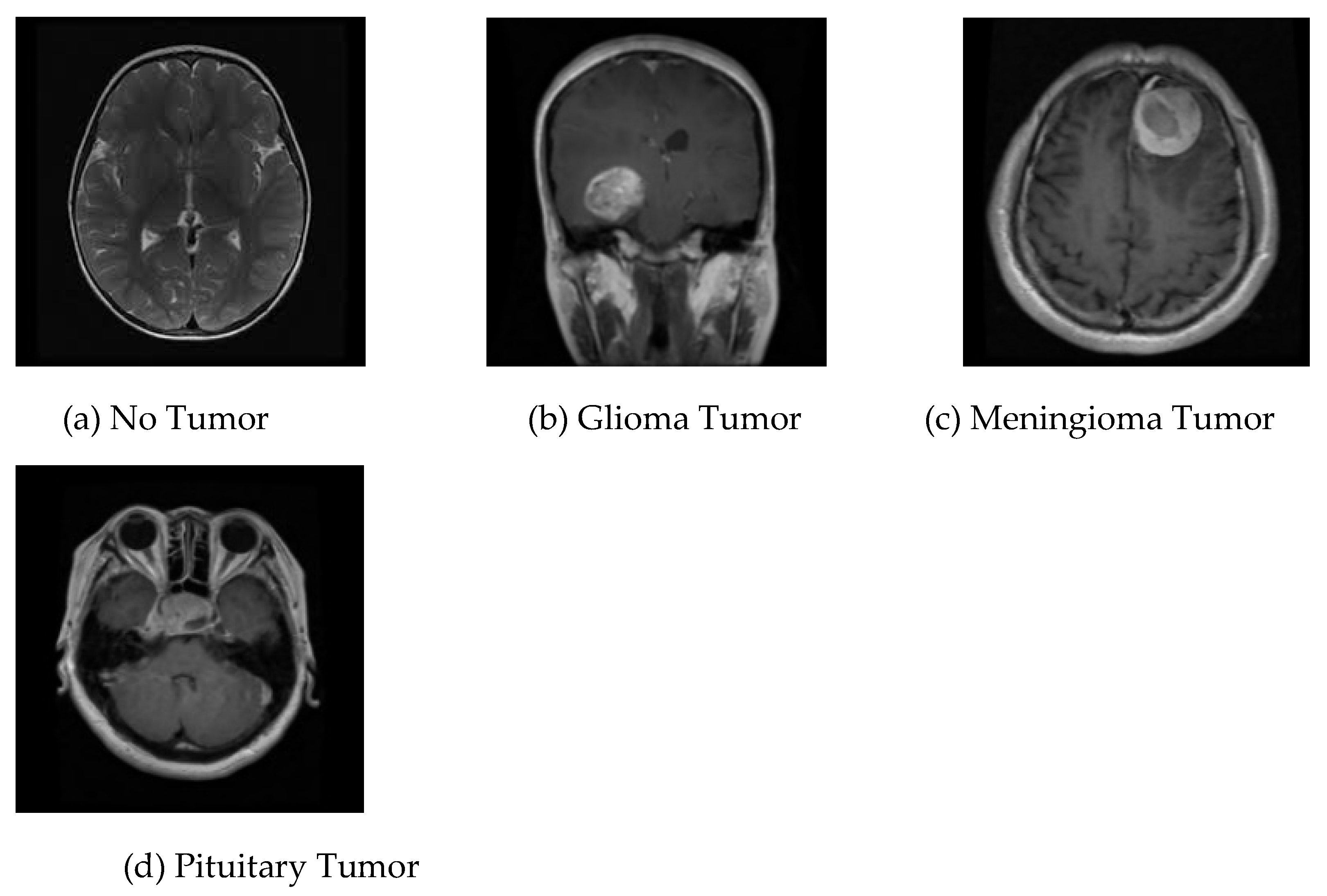
Figure 4.
Proposed architecture of dilated PDCNN model.
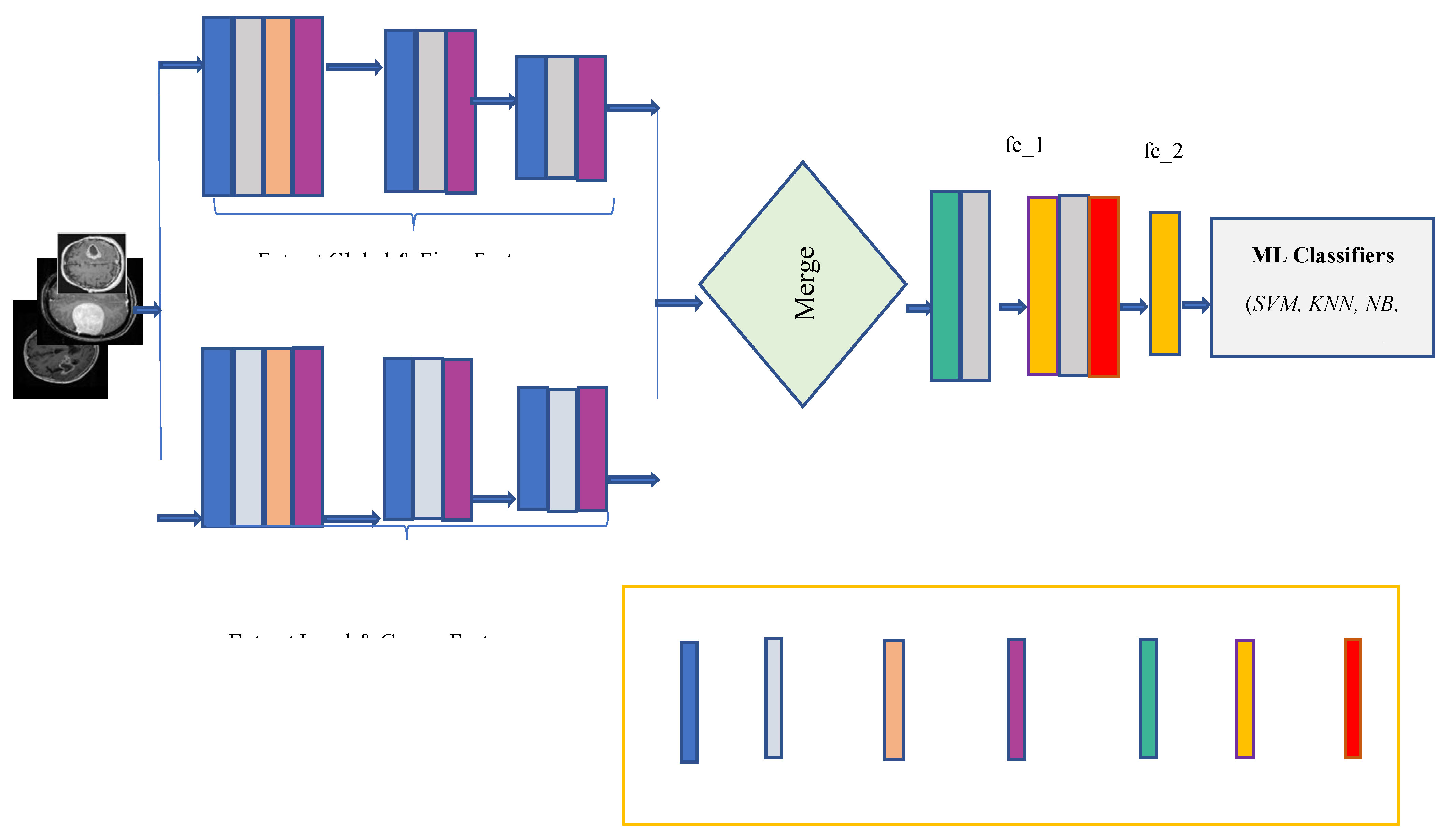
Figure 9.
Comparing accuracy across different configurations of dilation rates.
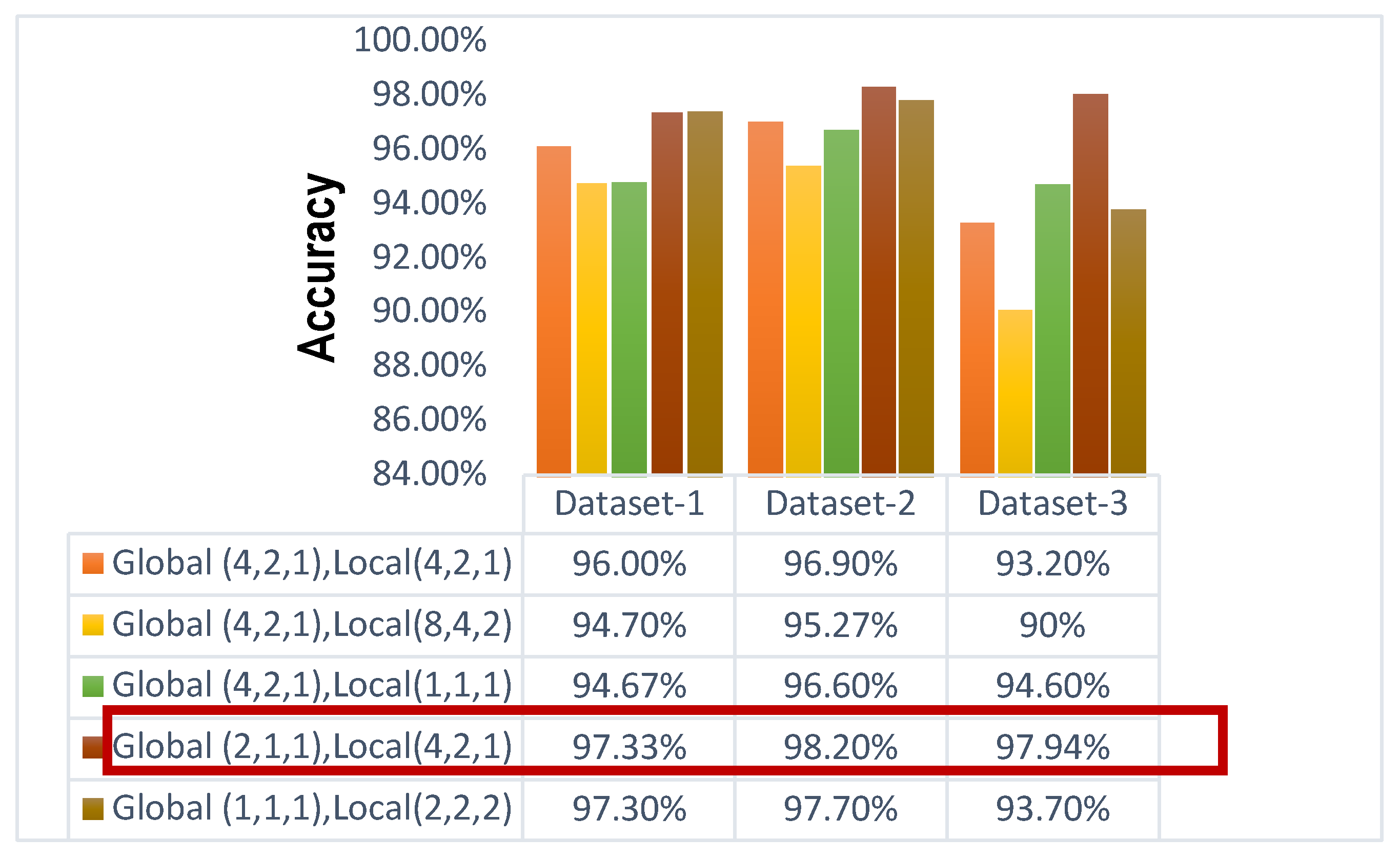
Figure 10.
Performance metrics comparison of (a) accuracy (b) precision (c) recall (d) F1-score (e) error rate (f) kappa and (g) execution time comparison along three types of brain tumor datasets.
Figure 10.
Performance metrics comparison of (a) accuracy (b) precision (c) recall (d) F1-score (e) error rate (f) kappa and (g) execution time comparison along three types of brain tumor datasets.
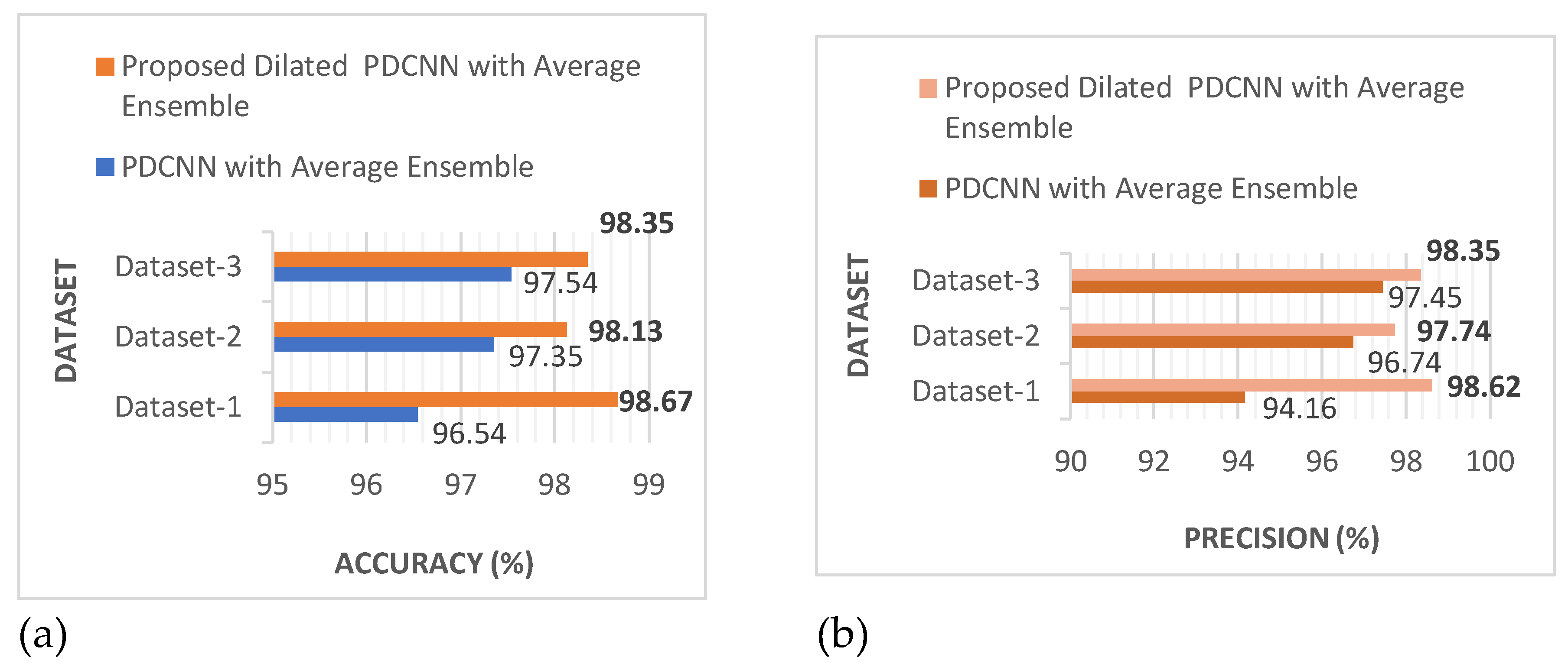
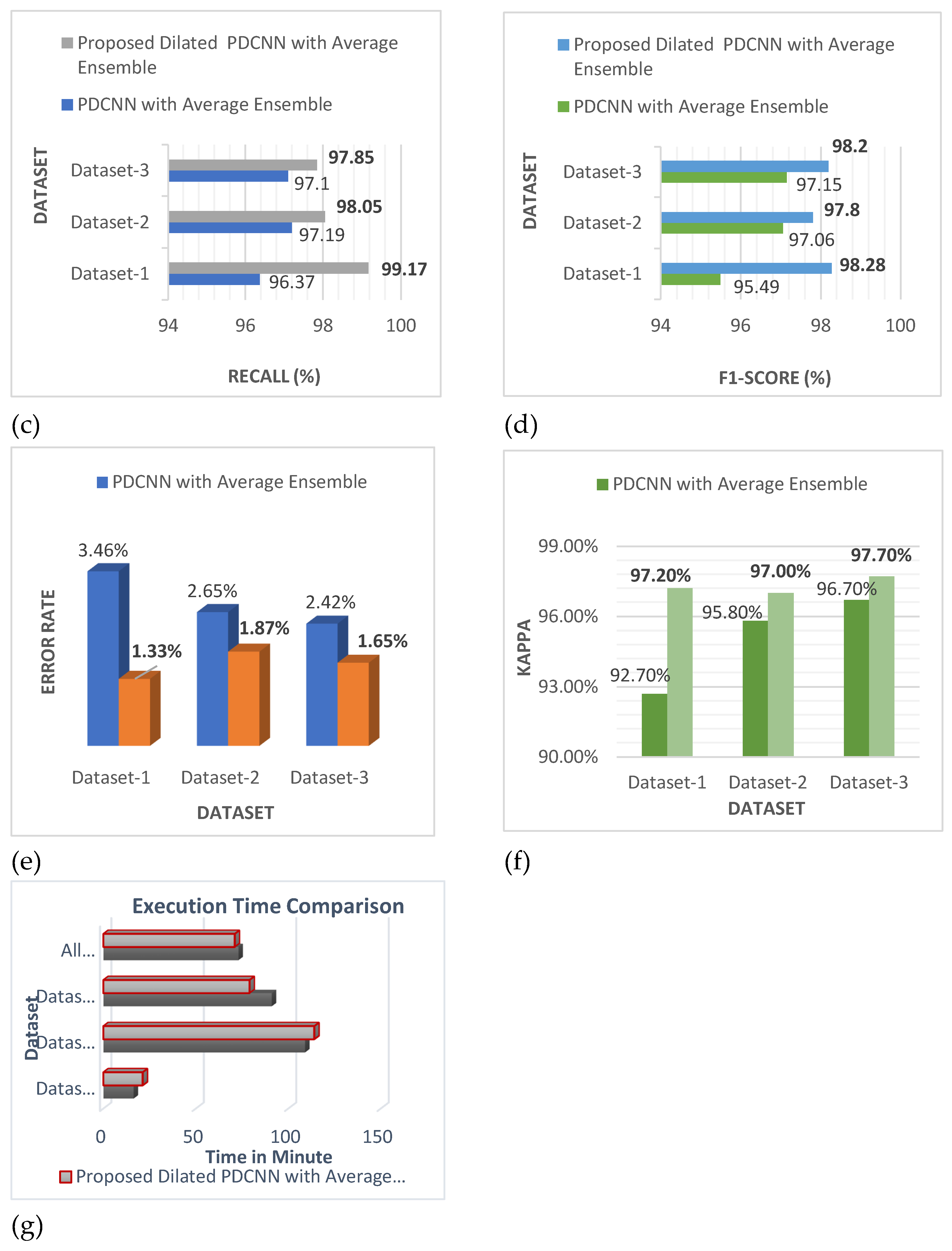
Table 5.
Performance Parameters of Dilated PDCNN Model with ML Classifiers on Dataset-Ⅰ.
| Dilated PDCNN Models Utilizing ML Classification | Accuracy (%) | Precision (%) | Recall (%) | F1-Score (%) |
|---|---|---|---|---|
| Dilated PDCNN | 97.33 | 93.10 | 95.83 | 96.43 |
| Dilated PDCNN with SVM | 98.67 | 100.00 | 100.00 | 98.31 |
| Dilated PDCNN with KNN | 100.00 | 100.00 | 100.00 | 100.00 |
| Dilated PDCNN with NB | 97.33 | 100.00 | 100.00 | 96.67 |
| Dilated PDCNN with Decision Tree | 100.00 | 100.00 | 100.00 | 100.00 |
| Dilated PDCNN with Average Ensemble | 98.67 | 98.62 | 99.17 | 98.28 |
Table 6.
Performance Parameters of Dilated PDCNN Model with ML Classifiers on Dataset-Ⅱ.
| Dilated PDCNN Models Utilizing ML Classification | Accuracy (%) | Precision (%) | Recall (%) | F1-Score (%) |
|---|---|---|---|---|
| Dilated PDCNN | 98.20 | 98.00 | 98.33 | 98.00 |
| Dilated PDCNN with SVM | 97.72 | 97.33 | 97.33 | 97.33 |
| Dilated PDCNN with KNN | 97.60 | 97.00 | 97.60 | 97.30 |
| Dilated PDCNN with NB | 98.90 | 98.67 | 98.67 | 98.67 |
| Dilated PDCNN with Decision Tree | 98.21 | 97.67 | 98.33 | 97.67 |
| Dilated PDCNN with Average Ensemble | 98.13 | 97.74 | 98.05 | 97.80 |
Table 7.
Performance Parameters of Dilated PDCNN Model with ML Classifiers on Dataset-Ⅲ.
| Dilated PDCNN Models Utilizing ML Classification | Accuracy (%) | Precision (%) | Recall (%) | F1-Score (%) |
|---|---|---|---|---|
| Dilated PDCNN | 98.21 | 98.25 | 97.75 | 98.25 |
| Dilated PDCNN with SVM | 98.60 | 98.50 | 98.25 | 98.50 |
| Dilated PDCNN with KNN | 98.50 | 98.50 | 98.00 | 98.50 |
| Dilated PDCNN with NB | 98.57 | 98.50 | 98.00 | 98.50 |
| Dilated PDCNN with Decision Tree | 97.85 | 98.00 | 97.25 | 97.25 |
| Dilated PDCNN with Average Ensemble | 98.35 | 98.35 | 97.85 | 98.20 |
Table 8.
Evaluation Results of the Proposed System on the Binary Classification Dataset-Ⅰ.
| Structure | Classifier | Performance Indicators | |||
| Accuracy (%) | Error (%) | Time (s) | Kappa | ||
| PDCNN | Custom PDCNN | 96.03 | 3.97 | 662 | 0.917 |
| PDCNN and SVM | 97.33 | 2.67 | 1020 | 0.943 | |
| PDCNN and KNN | 96.00 | 4.00 | 1069 | 0.915 | |
| PDCNN and NB | 94.67 | 5.33 | 1079 | 0.888 | |
| PDCNN and Decision Tree | 98.67 | 1.33 | 1070 | 0.972 | |
| Average Ensemble | 96.54 | 3.46 | 980 | 0.927 | |
| Dilated PDCNN | Custom PDCNN | 97.33 | 2.67 | 1683 | 0.943 |
| PDCNN and SVM | 98.67 | 1.33 | 1020 | 0.972 | |
| PDCNN and KNN | 100.00 | 0.00 | 1223 | 1.000 | |
| PDCNN and NB | 97.33 | 2.67 | 1223 | 0.944 | |
| PDCNN and Decision Tree | 100.00 | 0.00 | 1223 | 1.000 | |
| Average Ensemble | 98.67 | 1.33 | 1274 | 0.972 | |
Table 9.
Evaluation Results of the Proposed System on the Multiclass Figshare Dataset-Ⅱ.
| Structure | Classifier | Performance Indicators | |||
| Accuracy (%) | Error (%) | Time (s) | Kappa | ||
| PDCNN | Custom PDCNN | 97.64 | 2.36 | 8050 | 0.963 |
| PDCNN and SVM | 97.71 | 2.29 | 6106 | 0.960 | |
| PDCNN and KNN | 97.40 | 2.60 | 6307 | 0.959 | |
| PDCNN and NB | 97.40 | 2.60 | 4998 | 0.959 | |
| PDCNN and Decision Tree | 96.60 | 3.40 | 7170 | 0.946 | |
| Average Ensemble | 97.35 | 2.65 | 6526 | 0.958 | |
| Dilated PDCNN | Custom PDCNN | 98.20 | 1.80 | 7204 | 0.972 |
| PDCNN and SVM | 97.72 | 2.28 | 6106 | 0.962 | |
| PDCNN and KNN | 97.60 | 2.40 | 6187 | 0.961 | |
| PDCNN and NB | 98.90 | 1.10 | 6149 | 0.982 | |
| PDCNN and Decision Tree | 98.21 | 1.79 | 8381 | 0.972 | |
| Average Ensemble | 98.13 | 1.87 | 6805 | 0.970 | |
Table 10.
Evaluation Results of the Proposed System on the Multiclass Kaggle Dataset-Ⅲ.
| Structure | Classifier | Performance Indicators | |||
| Accuracy (%) | Error (%) | Time (s) | Kappa | ||
| PDCNN | Custom PDCNN | 96.80 | 3.20 | 5633 | 0.956 |
| PDCNN and SVM | 97.94 | 2.06 | 4462 | 0.972 | |
| PDCNN and KNN | 97.80 | 2.20 | 5753 | 0.969 | |
| PDCNN and NB | 97.90 | 2.10 | 5753 | 0.972 | |
| PDCNN and Decision Tree | 97.40 | 2.60 | 5753 | 0.965 | |
| Average Ensemble | 97.58 | 2.42 | 5470 | 0.967 | |
| Dilated PDCNN | Custom PDCNN | 98.21 | 1.79 | 4891 | 0.976 |
| PDCNN and SVM | 98.60 | 1.40 | 4739 | 0.980 | |
| PDCNN and KNN | 98.50 | 1.50 | 4739 | 0.979 | |
| PDCNN and NB | 98.57 | 1.43 | 4739 | 0.980 | |
| PDCNN and Decision Tree | 97.85 | 2.15 | 4739 | 0.971 | |
| Average Ensemble | 98.35 | 1.65 | 4769 | 0.977 | |
Table 11.
Assessment of the Employed Kaggle and Figshare Datasets with the Methods Currently in Use.
Table 11.
Assessment of the Employed Kaggle and Figshare Datasets with the Methods Currently in Use.
| No | Authors | Structure | Year | Data Type | Accuracy (%) |
|---|---|---|---|---|---|
| 1. | P. Afshar et al. [12] | Capsule Networks | 2019 | Figshare Dataset-Ⅱ | 90.89 |
| 2. | C. L. Choudhury et al. [35] | CNN | 2020 | Binary Dataset-Ⅰ | 96.08 |
| 3. | H. H. Sultan et al. [36] | Resize+ Augmentation + CNN + Hyperparameter Tuning | 2019 | Figshare Dataset-Ⅱ | 96.13 |
| 4. | Suhib et. al [18] | Gray Transformation + Resize + Flatten + CNN | 2020 | Binary Dataset-Ⅰ | 96.7 |
| 5. | A. E. Minarno et al. [21] | Resize+ Augmentation + CNN+ Hyperparameter Tuning | 2021 | Kaggle Dataset-Ⅲ | 96.00 |
| 6. | Priyansh et al. [37] | CNN-Based Transfer Learning Approach | 2021 | Binary Dataset-Ⅰ | Resnet-50-95, VGG-16- 90, Inception-V3-55 |
| 7. | T. Rahman et al. [38] | Resize+ Gray+ Augmen-tation+ Binary+ CNN | 2022 | Binary Dataset-Ⅰ | 96.9 |
| 8. | A. Biswas et al. [39] | Resize+ Anisotropic Diffusion Filter+ Adaptive Histogram Equalization+ DCNN-SVM | 2023 | Figshare Dataset-Ⅱ | 96 |
| 9. | H.A. Munira et al. [40] | Thresholding + Cropping+ Resizing+ Rescaling+ CNN-RE and CNN-SVM | 2022 | Figshare Dataset-Ⅱ Kaggle Dataset-Ⅲ |
CNN-RF-96.52 CNN-SVM-95.41 |
| 10. | T. Rahman et al. [34] | Resize + Gray Transformation + Augmentation + PDCNN | 2023 | Binary Dataset-Ⅰ | 97.33 |
| Figshare Dataset-Ⅱ | 97.60 | ||||
| Kaggle Dataset-Ⅲ | 98.12 | ||||
| 11. | Proposed Method | Resize + Gray scale Transformation+ Augmentation + Dilated PDCNN+ Machine Learning Classifiers+ Average Ensemble | - | Binary Dataset-Ⅰ | 98.67 |
| Figshare Dataset-Ⅱ | 98.13 | ||||
| Kaggle Dataset-Ⅲ | 98.35 |
Disclaimer/Publisher’s Note: The statements, opinions and data contained in all publications are solely those of the individual author(s) and contributor(s) and not of MDPI and/or the editor(s). MDPI and/or the editor(s) disclaim responsibility for any injury to people or property resulting from any ideas, methods, instructions or products referred to in the content. |
© 2024 by the authors. Licensee MDPI, Basel, Switzerland. This article is an open access article distributed under the terms and conditions of the Creative Commons Attribution (CC BY) license (http://creativecommons.org/licenses/by/4.0/).
Copyright: This open access article is published under a Creative Commons CC BY 4.0 license, which permit the free download, distribution, and reuse, provided that the author and preprint are cited in any reuse.


