Submitted:
05 May 2024
Posted:
06 May 2024
You are already at the latest version
Abstract
This study assesses the predictive performance of six machine learning models in forecasting tumor dynamics within three months following Gamma Knife Radiosurgery (GKRS) in 77 brain metastasis (BM) patients. The analysis meticulously evaluates each model before and after hyperparameter tuning, utilizing accuracy, AUC and other metrics derived from confusion matrices. Initial findings highlighted that XGBoost significantly outperformed other models with an accuracy of 0.95 and an AUC of 0.95 before tuning. Post-tuning, the Support Vector Machine (SVM) demonstrated the most substantial improvement, achieving an accuracy of 0.98 and an AUC of 0.98. Conversely, XGBoost showed a decline in performance after tuning, indicating potential overfitting. The study also explores feature importance across models, noting that features like “control at one year”, “age of the patient”, and “beam on time for volume V1 treated”, were consistently influential across various models, albeit their impacts were interpreted differently depending on the model’s underlying mechanics. This comprehensive evaluation not only underscores the importance of model selection and hyperparameter tuning but also highlights the practical implications in medical diagnostic scenarios, where the accuracy of positive predictions can be crucial.
Keywords:
gamma knife radiosurgery (GKRS)
; brain metastasis
; tumor dynamics forecasting
; machine learning models
; feature importance
1. Introduction
Brain metastases (BM), often referred to as secondary brain cancers, pose significant treatment dilemmas and urgently need strategies to lessen the impact on those diagnosed [1]. There’s an increasing incidence of BM, likely influenced by improvements in conventional therapies like surgery, radiation, and chemotherapy, which have led to longer survival rates for patients. Without any medical interventions, people with BM usually face a median survival time of approximately 2 months after their diagnosis, especially when the disease affects the central nervous system [2]. The advent of targeted treatment methods, such as gamma knife radiosurgery (GKRS), is becoming a preferred approach for BM management due to its ability to better target tumors locally with fewer side effects compared to traditional whole brain radiation therapy, and its effectiveness is on par with that of surgical removal [3,4,5,6]. However, GKRS is limited in treating larger BM (exceeding 3 cm in diameter or 10 cc in volume) because of the potential for radiation-induced harm, like radiation toxicity [7,8,9,10]. The Gamma Knife ICON, using mask fixation for patient positioning, represents an advanced solution for hypo-fractionated treatment of large BM. Despite these advancements, the median survival rate for patients with BM hovers around one year [11,12].
Lung cancer stands as a major global cancer threat, categorized mainly into non-small cell lung cancer (NSCLC) and small cell lung cancer. NSCLC is further divided into adenocarcinoma, squamous cell carcinoma, and large cell carcinoma, as classified by the World Health Organization [13,14]. Between 30% and 40% of those with NSCLC experience brain metastases (BM) [15,16,17]. For these patients, gamma knife radiosurgery (GKRS) has been acknowledged as an effective and low-risk treatment method [18,19], although their median overall survival (OS) tends to be around one year [18,20]. The outlook for NSCLC patients facing BM remains bleak, with approximately 10% dying within two months following their diagnosis [21,22]. The use of GKRS for NSCLC patients with BM is debated due to their limited OS. Nevertheless, some policies, like those implemented in Korea, permit the use of GKRS for BM treatment every three months.
Beyond lung cancer, other cancers such as breast, colorectal, prostate, ovarian, and renal cancers also frequently metastasize to the brain, significantly impacting patient outcomes and treatment approaches. Breast cancer, for example, has a notable propensity to spread to the brain, particularly in patients with HER2-positive or triple-negative subtypes, challenging clinicians to tailor treatments for both systemic disease and brain involvement [23]. Colorectal cancer, though less commonly associated with BM, poses a significant risk when metastasis occurs, necessitating a multidisciplinary approach to manage both the primary disease and brain metastases [24]. Prostate cancer rarely metastasizes to the brain, but when it does, it signifies a late-stage disease and poor prognosis, highlighting the need for innovative therapeutic strategies [25,26]. Ovarian and renal cancers, similarly, can lead to brain metastases, with renal cell carcinoma being more prone to spread to the brain, requiring careful consideration of treatment options to address this aggressive disease behavior [27,28].
In the realm of clinical decision-making, consensus agreements and expert recommendations often guide actions, especially in scenarios where evidence might be scarce [29]. Simplifying information structures aids in modeling observations and facilitating conclusion formulation [30]. Machine learning (ML), as a branch of artificial intelligence, is instrumental in crafting models that learn from data autonomously, without direct programming. Among these, tree-based ML algorithms are particularly appreciated for their straightforwardness and clarity, making the decision paths visual and interpretable. Decision trees stand out by mapping decisions through nodes and labels, ensuring not only high accuracy in classification but also clear presentation of information, which is crucial in healthcare decision-making [31,32]. However, challenges such as overfitting can arise from small data sets. Techniques like random forests and boosted decision trees are therefore employed to overcome these hurdles, offering improved prediction accuracy by a detailed examination of the interconnections among variables in the dataset [33]. This is why, in our investigation of patients experiencing brain metastases from various primary cancers, we used in addition to the usual ML algorithms, such as Logistic Regression, Support Vector Machines (SVM) and K nearest neighbors (KNN), tree-based modeling techniques—including Decision Tree, Random Forest, and Boosted decision tree classifiers XGBoost - to anticipate the dynamics of tumors within 3 months following GKRS treatment. This approach allowed us to pinpoint essential factors and feature permutations that are crucial in estimating the prognosis for these patients.
2. Research Methodology
2.1. Overview of Research Design and Participant Details
We outline the framework of our study, detailing the procedures followed and the characteristics of the individuals who participated in our research.
The study protocol retrospectively reviewed the medical records of patients treated with GKRS, with mask-based fixation, of BM from various primary cancers, between July 2022 and March 2024 at "Prof. Dr. Nicolae Oblu" Emergency Clinic Hospital – Iasi. All experiments were carried out in accordance with relevant guidelines and regulations. The study used only pre-existing medical data, therefore patient consent was not required, and since it was retrospective, there was no need of approval from the Ethics Committee of Clinical Emergency Hospital "Prof. Dr. Nicolae Oblu" Iasi.
A total of 77 patients (45 males and 32 females; age range 39 to 85 years old; median age, 64 years old) who were previously diagnosed with BM were enrolled in this study. General characteristics including age, sex, C1yr – tumor volume at one year control, MTS extra cranial – existence of extra cranial metastases, receiving pretreatment, deceased before 1 year, Karnofsky performance scale (KPS) score [34], number of lesions, beam on time over the number of isocenters for each of the 3 volumes treated, total tumor volume and tumor dynamics (progression or regression within 3 months following GKRS treatment), were summarized in Table 1. The study design was shown in Figure 1.
2.2. Strategy for Gamma Knife Radiosurgery Implementation
We discuss in what follows, the systematic approach adopted for administering Gamma Knife Radiosurgery (GKRS), focusing on the meticulous planning and execution phases essential for the treatment. All patients underwent GKRS using the Leksell Gamma Knife ICON (Elekta AB, Stockholm, Sweden).
All MRI examinations were performed on a 1.5 Tesla whole-body scanner (GE 174 SIGMA EXPLORER) that was equipped with the standard 16-channel head coil. The MRI 175 study protocol consisted of:
1. The conventional anatomical MRI (cMRI) protocol for clinical routine diagnosis of brain tumors, included among others, an axial fluid-attenuated inversion recovery (FLAIR) sequence, as well as a high-resolution contrast-enhanced T1-weighted (CE T1w) sequence.
2. The advanced MRI (advMRI) protocol for clinical routine diagnosis of brain tumors was extended by axial diffusion-weighted imaging (DWI; b values 0 and 1000 s/mm2) sequence and a gradient echo dynamic susceptibility contrast (GE-DSC) perfusion MRI sequence, which was performed using 60 dynamic measurements during administration of 0.1 mmol/kg-bodyweight gadoterate-meglumine.
All magnetic resonance images were registered with Leksell Gamma Plan (LGP, Version 11.3.2, TMR algorithm), and any images with motion artifacts were excluded. The tumor volumes were calculated by LGP without margin. Generally, the prescription of a total dose of 30 Gy delivered in 3 stages GRKS, was selected based on the linear quadratic model [35,36] and the work of Higuchi et al. from 2009 [37]. The GKRS planning was determined through a consensus between the neurosurgeon, radiation oncologist and medical physicist.
2.3. Labeling of Medical Data
In the process of labeling medical data, we extracted relevant features from the broad details available in the electronic medical record (EMR) system. One of the prevalent hurdles in machine learning (ML) applications is the issue of incomplete data within the EMR. To tackle this, we applied two principal strategies: imputation and exclusion of data.
Imputation is the method of filling in missing information with plausible values, which proves particularly beneficial when the missing data is scarce. In our research, we opted to replace missing entries in categorical data with the value found in the previous row, whereas for numerical attributes, we used the median value of the dataset. Additionally, for the transformation of categorical variables, label encoding techniques were utilized [38].
Unbalanced datasets pose challenges in ML when one class vastly outweighs others, which is the case of our study, only 6 patients in 77 (7.8%) showed signs of progression of lesions (see Figure 3). Approaches to address this issue include resampling (oversampling/undersampling), class weighting, cost-sensitive learning, ensemble methods, and data augmentation. The appropriate method depends on the problem and dataset, necessitating evaluation on all classes for accurate results [39,40,41,42,43].
2.4. Data Manipulation Techniques
Our preference for the Python programming language in this study was driven by its simplicity in handling data operations, coupled with its access to a broad spectrum of freely available libraries [44]. The project leveraged the capabilities of open-source Python 3.0 libraries, including NumPy for numerical data manipulation, pandas for data structures and analysis, Matplotlib and seaborn for data visualization, and TensorFlow, Keras, and scikit-learn for machine learning and data mining tasks.
Logistic Regression is effective in handling binary outcomes, such as the presence or absence of tumor growth. It can utilize various patient and tumor characteristics to predict the probability of specific outcomes, aiding in the risk stratification and management of patients. Support Vector Machines excels in classifying complex patient data into distinct categories, such as predicting the likelihood of tumor recurrence. Its ability to handle high-dimensional data makes it invaluable in analyzing the myriad factors influencing brain metastases, from genetic markers to treatment responses. K Nearest Neighbors offers a straightforward yet powerful method for prognosis by comparing a patient’s data against those of similar patients. This similarity-based approach is especially beneficial in medical cases where individual patient characteristics significantly influence the disease trajectory, allowing for personalized prediction of tumor dynamics. Together, Decision Trees and Random Forest algorithms harness the intricate data landscape of BM to deliver nuanced and individualized prognostic insights. They enable a structured analysis of the factors driving tumor behavior, facilitating targeted and evidence-based treatment strategies that can lead to better patient management and outcomes. [45,46]. XGBoost is a machine learning algorithm that belongs to the ensemble learning category, specifically the gradient boosting framework. It utilizes decision trees as base learners and employs regularization techniques to enhance model generalization. Known for its computational efficiency, feature importance analysis, and handling of missing values, XGBoost is widely used for tasks such as regression, classification, and ranking, therefore it was a key component of our methodology [47]. The dataset was randomly divided into training group (n = 54) and test group (n = 23). We typically adhere to the conventional 80:20 training-to-test set ratio. However, due to the limited volume of data at our disposal, we opted to modify this ratio (70:30) to ensure a more robust evaluation of the test set performance. This adjustment allows for a more comprehensive assessment under constrained data conditions. The input variables were general characteristics. Hyperparameter tuning was conducted using the GridSearchCV function from scikit-learn, targeting the optimization of model parameters. The dependent variable under investigation was tumor dynamics, i.e. progression or regression within 3 months following GKRS treatment, categorized into "Regression" or "Progression."
To assess the performance of the ML algorithm models, we computed metrics such as accuracy, sensitivity, specificity, along with the receiver operating characteristic (ROC) curve and the area under the curve (AUC). Subsequent to model training, we identified and validated important features and permutation features, with permutation feature importance serving as a versatile technique for evaluating the significance of features across various fitted models, provided the data is structured in tabular form [48].
3. Results
3.1. Overview of Data
The cohort study included 77 patients with BM, focusing on their age at the time of GKRS treatment. KPS scores were evaluated by physicians. Pathologic diagnoses, receiving chemotherapy, and pretreatment records were obtained from EMR. The number of lesions, tumor volume, the number of fractions, and prescription doses were documented in the LGP. Detailed data descriptions are summarized in Table 2.
Let us interpret the information in the bar charts from Figure 2a. Each chart shows the distribution of patients with tumor regression (label ’0’) versus tumor progression (label ’1’) across different variables within a dataset, possibly from a medical study on cancer.
1. Sex (Gender):
- The chart shows that among females (’F’), tumor regression (no progression) is more common than progression.
- Among males (’M’), the situation is quite different, with tumor progression being significantly more prevalent than regression.
- This may suggest that in this specific dataset or condition, males are at a higher risk of tumor progression compared to females.
2. Mts_ext (Presence of External Metastases):
- Patients without external metastases (label ’0’) show a lower rate of tumor progression.
- In contrast, the presence of external metastases (label ’1’) correlates with a much higher count of tumor progression.
- This suggests that external metastases are a strong indicator of tumor progression within this patient population.
3. T_sist (Pre-treatment):
- A smaller number of patients who did not receive pre-treatment (label ’0’) show regression.
- A larger number of patients who did receive some form of pre-treatment (label ’1’) also exhibit tumor progression
- Although it seems counterintuitive that more pre-treated patients have tumor progression, this could be due to a variety of factors, such as the severity of the cancer at the time of treatment. It could also be that patients who are more likely to progress are also more likely to receive pre-treatment.
4. Dec_1yr (Deceased within One Year):
- There is a much higher count of patients who have not deceased within one year (label ’0’) showing tumor regression.
- A smaller number of patients who deceased within one year (label ’1’) show a correlation with tumor progression.
- This indicates that tumor progression is likely associated with higher mortality within one year in this dataset.
These charts collectively offer valuable insights into factors associated with tumor progression and survival rates in patients. For instance, gender differences and the presence of external metastases are prominently associated with the progression of the tumor. Pre-treatment status is less clear-cut and could be influenced by many factors that the chart does not specify. Finally, the strong correlation between tumor progression and one-year mortality underscores the seriousness of tumor progression as an indicator of patient prognosis. It’s important to note that these are correlative relationships, and causation should not be inferred without further, controlled study.
The eight box-plots in Figure 2b show the distribution of various medical variables for two groups of patients: those with tumor regression (label ’0’) and those with tumor progression (label ’1’). Let’s discuss each one:
1. Age:
- The age distributions for both groups overlap significantly, with a median age slightly higher for the group with tumor progression (label ’1’).
- There are outliers in both groups, suggesting some patients with extreme ages compared to the rest.
2. C1_yr (Tumor Volume at 1 Year Control):
- Patients with tumor regression have lower tumor volumes at 1-year control (tighter distribution and lower median), while those with progression have higher volumes (wider distribution and higher median).
- There are outliers in both groups, which may represent atypical cases or measurement errors.
3. Karn (Karnofsky Performance Status):
- Patients with tumor regression have generally higher Karnofsky scores, indicative of better functional status or ability to carry out daily activities without assistance.
- Patients with tumor progression have a lower median score and a wider distribution, indicating more variability in their functional status.
4. Nr_Mts (Number of Metastases):
- Patients with tumor regression tend to have fewer metastases, as indicated by the lower median and more compact box-plot.
- Those with tumor progression have a higher median number of metastases and a wide range, with several outliers indicating some patients have a very high number of metastases.
5. B_on1 (Beam On Time for Volume 1 Treated):
- This plot shows a slight increase in the beam on time for patients with tumor regression compared to those with progression for volume 1 treated.
- There are a few outliers in the group with regression, indicating some treatments with exceptionally long beam times.
6. B_on2 (Beam On Time for Volume 2 Treated):
- The beam on time for volume 2 treated does not seem to differ significantly between the two groups.
- Both groups show outliers, suggesting variations in treatment time not necessarily related to tumor progression.
7. B_on3 (Beam On Time for Volume 3 Treated):
- The box-plot for patients with tumor progression is more compact for beam on time for volume 3, while there’s more variability among those with tumor regression.
- Outliers are present in both groups, with the group with regression having more extreme cases.
8. Vol_tum (Total Volume of the Tumor):
- Patients with tumor regression have a lower median tumor volume and a tighter distribution, suggesting smaller tumors overall.
- Those with tumor progression show a wider distribution and a higher median, indicating larger tumors.
In summary, patients with tumor regression generally have lower volumes of tumor at control, fewer metastases, and higher Karnofsky scores, while those with progression show opposite trends. The beam on time seems to vary less consistently between the groups, with some outliers indicating individual variability in treatment. These box-plots provide a visual summary of how these variables correlate with tumor outcomes in the study population.
3.2. Analysis of ML Models
Before hyperparameters tuning
Table 3 shows the performance metrics for six different predictive models on our dataset. Two key performance metrics are reported: Accuracy and the Area Under the Receiver Operating Characteristic Curve (AUC).
1. Logistic Regression, SVM (Support Vector Machine), Decision Tree, and Random Forest:
- These four models all have identical accuracy and AUC scores of approximately 0.930 and 0.93, respectively. This could suggest that the dataset and features used may not be complex enough to differentiate the performance of these models, or that the default hyperparameters of these models happen to perform similarly on this dataset.
2. KNN (K-Nearest Neighbors):
- The KNN model has a lower accuracy (0.8837) and AUC (0.89) compared to the other models. This may be due to the nature of KNN, which makes predictions based on the labels of the nearest training examples. KNN is often more sensitive to the scale of the data and the choice of ’k’ (the number of neighbors). Without tuning, KNN can perform poorly if the default ’k’ is not suitable for the dataset.
3. XGBoost (eXtreme Gradient Boosting):
- XGBoost outperforms all other models with the highest accuracy (0.9535) and AUC (0.95). This model uses gradient boosting, which is an ensemble technique that builds the model in a stage-wise fashion and is typically strong in handling varied types of data and relationships.
The fact that all models except KNN have very similar accuracy and AUC scores might indicate that the models are all capturing a strong signal in the data. The high performance across multiple models could also imply that the task or the data is not very challenging for these models, or that these models have reached a performance plateau on this dataset.
However, it’s important to note that these results are based on un-tuned models. Performance could change with hyperparameter tuning. Additionally, while accuracy and AUC are common metrics for evaluating classification models, they don’t tell the whole story. For example, if the dataset is imbalanced, accuracy might not be as informative and other metrics like precision, recall, and the F1 score could be more relevant.
Moreover, depending on the cost of false positives or false negatives in the practical application of these models (such as medical diagnostics or fraud detection), one might prefer a model with a better balance between sensitivity (true positive rate) and specificity (true negative rate), which can be assessed with the AUC metric. Since the AUCs are high and close across most models, it suggests they all have a good balance between sensitivity and specificity, with XGBoost being slightly better.
Figure 4 shows the confusion matrices for the six predictive models tested without tuning: Logistic Regression, SVM (Support Vector Machine), KNN (K-Nearest Neighbors), Decision Tree, Random Forest, and XGBoost.
The confusion matrix is a performance measurement for machine learning classification. It is a table with four different combinations of predicted and actual values:
- True Negatives (TN): The model correctly predicts the negative class.
- False Positives (FP): The model incorrectly predicts the positive class.
- False Negatives (FN): The model incorrectly predicts the negative class.
- True Positives (TP): The model correctly predicts the positive class.
Here’s an interpretation of each matrix:
1. Logistic Regression, SVM, Decision Tree, Random Forest:
- All four of these models have the same confusion matrix, with 19 true negatives (TN), 3 false positives (FP), 0 false negatives (FN), and 21 true positives (TP). This indicates that they are performing identically in terms of true/false positives/negatives.
- The absence of false negatives suggests that these models are very sensitive to the positive class, capturing all positive instances without fail.
2. KNN:
- The KNN model has 17 TN, 5 FP, 0 FN, and 21 TP. It has more false positives than the other four models but still no false negatives, meaning it is still sensitive but less precise.
3. XGBoost:
- The XGBoost model has 20 TN, 2 FP, 0 FN, and 21 TP. It has the highest number of true negatives and the lowest number of false positives, making it the most accurate and precise model among those tested.
- Like the other models, XGBoost has no false negatives, maintaining high sensitivity.
Key Points:
- All models have high sensitivity (no false negatives), which is crucial in many applications, particularly in medical diagnoses where missing a positive case can have severe consequences.
- XGBoost stands out with the highest precision (fewest false positives) and would be the most reliable model in this case for minimizing incorrect positive predictions.
- The identical performance of Logistic Regression, SVM, Decision Tree, and Random Forest suggests that for this specific dataset and problem, the choice between these models might not matter much in terms of true/false positives/negatives.
- KNN has slightly lower precision, with more false positives than the other models, indicating that it might be less suitable for this specific dataset or task without further tuning.
- It’s also worth noting that all models have a relatively high number of true positives, which suggests that the dataset might be balanced, or that the models are effectively identifying the positive class.
The Receiver Operating Characteristic (ROC) curves in Figure 5 compare the diagnostic ability of the six classification models at various threshold settings. The Area Under the Curve (AUC) for each model is a summary measure of the accuracy of the test. Here are the insights based on the provided ROC curves:
1. SVM and Random Forest:
- Both have a perfect AUC of 1.00, which indicates exceptional classifier performance. In practical terms, these models have managed to separate the positive and negative classes without any overlap. However, in real-world data, such perfect scores are rare and might warrant further investigation for overfitting or data leakage.
2. XGBoost:
- With an AUC of 0.99, XGBoost also shows excellent performance, nearly perfect in separating the two classes. It is only marginally less perfect than SVM and Random Forest according to the AUC.
3. KNN:
- KNN has an AUC of 0.98, which is also very high, indicating that it is a strong classifier. Despite its lower performance in accuracy and a higher number of false positives as seen in the confusion matrix, the ROC curve suggests that KNN does well overall in distinguishing between the classes.
4. Logistic Regression and Decision Tree:
- These models have AUC scores of 0.92 and 0.93, respectively. While not as high as the others, these are still good scores, indicating that both models have a good measure of separability between the classes.
The ROC curve is a plot of the true positive rate (sensitivity) against the false positive rate (1-specificity) for the different possible cut points of a diagnostic test. A model with perfect prediction would have a point in the upper left corner of the ROC space, with coordinates (0,1), indicating 100% sensitivity (no false negatives) and 100% specificity (no false positives). The 45-degree dashed line represents the strategy of random guessing, and any model that lies above this line is considered to have some ability to separate the classes better than random chance.
Considering the ROC curves and the AUC scores, all models seem to perform well, with SVM and Random Forest appearing to be perfect classifiers according to these metrics. However, caution is advised because perfect classification is unusual and could indicate issues such as overfitting, especially if the models were not tuned. It’s also possible that the dataset is not challenging for the models, or there could be some feature that perfectly separates the classes which could be an artifact of the data collection process.
The classification report in Table 4, offers insights into the performance of six different machine learning models (Logistic Regression, SVM, KNN, Decision Tree, Random Forest, and XGBoost) without hyperparameter tuning. Here’s a detailed comment on each:
1. Logistic Regression, SVM, Decision Tree, and Random Forest:
- These models show remarkably similar performance metrics, each achieving an accuracy of 0.93.
- They all demonstrate high precision and recall for both classes (0 and 1), with class 1 always reaching a recall of 1.00 and precision varying slightly.
- The F1-score for both classes is 0.93 across these models, indicating a balanced performance between precision and recall.
2. KNN:
- This model has slightly lower overall performance compared to the other models, with an accuracy of 0.88.
- It displays a recall of 1.00 for class 1 but only 0.77 for class 0, suggesting it’s better at identifying class 1 instances.
- The precision for class 0 is excellent at 1.0, yet for class 1, it’s lower at 0.81.
- The macro and weighted averages for precision, recall, and F1-score are lower than those of the other models, reflecting its lesser overall effectiveness.
3.XGBoost:
- XGBoost shows the best performance among all models, with an accuracy of 0.95.
- It has an impressive recall of 1.00 for class 1 and the highest recall for class 0 (0.91) among all models.
- Precision and F1-scores are consistent at 0.95 for both classes, suggesting a very strong predictive capability.
- The macro and weighted averages are slightly higher than for other models, underscoring its superior performance.
Overall, these results highlight that XGBoost, even without hyperparameter tuning, outperforms other models in terms of accuracy, precision, recall, and F1-score. Meanwhile, the KNN model trails slightly behind, especially in terms of recall for class 0 and overall accuracy. These outcomes can serve as a baseline for further tuning and optimization of model parameters, which could potentially improve these metrics further.
After hyperparameters tuning
Table 5 presents the accuracy and AUC (Area Under the ROC Curve) scores for six machine learning models after they have undergone hyperparameter tuning. Tuning the models typically involves adjusting various parameters to improve performance.
Here’s an interpretation of the performance metrics after tuning:
1. Logistic Regression:
- The accuracy and AUC are both 0.95, which is a high score, indicating that the model is performing very well post-tuning.
2. SVM (Support Vector Machine):
- SVM shows the highest accuracy (0.9767) and a very high AUC (0.98) among all the models. This suggests that the tuning process was particularly effective for this model, making it the top performer in this set.
3. KNN (K-Nearest Neighbors):
- The accuracy and AUC for KNN are both 0.95, identical to the logistic regression model. This marks a significant improvement from the pre-tuning stage, especially in its AUC score.
4. Decision Tree:
- The decision tree has an accuracy of 0.9069 and an AUC of 0.91. Although these scores are the lowest among the models after tuning, they are still indicative of a good predictive ability.
5. Random Forest:
- Post-tuning, the random forest model has an accuracy of 0.9302 and an AUC of 0.93. These scores are solid but represent a slight decrease compared to the pre-tuning performance, suggesting that the model was potentially overfitted before tuning and has now generalized better.
6. XGBoost:
- Surprisingly, the XGBoost model shows a decrease in performance after tuning, with the lowest accuracy (0.8837) and AUC (0.89) of all the models. This is unusual, as XGBoost is known for benefiting from hyperparameter tuning. This could suggest that the tuning process may not have been optimal or that the model has overfit the training data to a degree.
Overall, it’s clear that hyperparameter tuning had a diverse impact on the performance of the models. While SVM, Logistic Regression, and KNN improved or maintained high performance, the Random Forest model had a slight decline, and XGBoost notably decreased in performance. This highlights the importance of careful tuning, as well as the possibility that some models might be more sensitive to the tuning process or that their default parameters were already close to optimal for the given dataset.
Figure 6 shows the confusion matrices for the six models tested after hyperparameter tuning. A confusion matrix is a table used to describe the performance of a classification model on a set of data for which the true values are known. It contains information about the actual and the predicted classifications done by a classification system. Performance of such models is commonly evaluated using the metrics derived from the confusion matrix, such as accuracy, precision, recall, and F1 score.
Here’s an interpretation of each confusion matrix after tuning:
1. Logistic Regression:
- The model predicted 20 instances correctly as class ’0’ and 21 instances correctly as class ’1’, with only 2 instances of class ’0’ incorrectly predicted as class ’1’ (false positives). There are no false negatives (instances of class ’1’ incorrectly predicted as class ’0’).
2. SVM (Support Vector Machine):
- SVM shows the highest precision with 21 true negatives and 21 true positives, and only 1 false positive. Like Logistic Regression, there are no false negatives.
3. KNN (K-Nearest Neighbors):
- Post-tuning, KNN has 20 true negatives and 21 true positives, with 2 false positives and no false negatives. This model also shows high precision and sensitivity.
4. Decision Tree:
- The Decision Tree model predicted 18 true negatives and 21 true positives, but with 4 false positives. It still correctly identifies all true positive instances without any false negatives.
5. Random Forest:
- Random Forest has 19 true negatives and 21 true positives, with 3 false positives. This model has no false negatives.
6. XGBoost:
- XGBoost shows 18 true negatives and 20 true positives but has 4 false positives and 1 false negative. This indicates a slight reduction in both precision and sensitivity compared to the other models.
After tuning, most models are performing very well, with high true positive rates and low false positives. It’s quite notable that almost all models have no false negatives, which is essential in critical applications where missing a positive instance (class ’1’) can be very costly or dangerous. SVM stands out as the model with the best performance, having the highest number of true positives and true negatives and the lowest number of false positives. In contrast, while still performing well, the Decision Tree and XGBoost have more false positives, and XGBoost additionally has a false negative, making them slightly less accurate than the others.
In summary, the tuning process seems to have optimized the models quite effectively, with some variations in the degree of improvement across different models. The performance is generally high, which is promising for the application of these models to the task at hand.
The provided Figure 7 shows the ROC (Receiver Operating Characteristic) curves for six models after hyperparameter tuning. The ROC curve is a graphical representation of a classifier’s diagnostic ability, plotting the true positive rate (sensitivity) against the false positive rate (1 - specificity) at various threshold settings.
Here are the insights from the ROC curves post-tuning:
1. SVM (Support Vector Machine) and Random Forest:
- Both these models have an AUC (Area Under the Curve) of 1.00, which suggests perfect classification with no overlap between the positive and negative classes. This is an ideal scenario, but it might also indicate overfitting, especially if the data is not very challenging or if there’s a ’leakage’ from the training data to the test data.
2. Logistic Regression:
- The model has an AUC of 0.95, indicating a high level of separability between classes and a strong performance.
3. KNN (K-Nearest Neighbors):
- The KNN model has an AUC of 0.98, which shows a high level of class separation and is a significant improvement over its pre-tuning performance.
4. Decision Tree:
- With an AUC of 0.93, the Decision Tree model’s performance is good but not as high as the other models. This might be due to its tendency to overfit, although tuning should have mitigated this to some extent.
5. XGBoost:
- XGBoost’s AUC of 0.98 is excellent, indicating very effective class separation. This contrasts with its performance in terms of accuracy and suggests it might have been less precise at the specific threshold used for the confusion matrix but still has a strong overall ability to rank positive instances higher than negative ones.
The dashed line represents random chance (AUC = 0.5), and all models perform significantly better than this baseline. A model’s ability to discriminate between the positive and negative classes increases as the ROC curve moves towards the upper left corner of the plot (higher true positive rate, lower false positive rate).
Given these AUC values, it’s clear that the tuning process has generally improved the models’ abilities to distinguish between classes, though the perfect AUC scores for SVM and Random Forest should be scrutinized for potential overfitting. AUC is a particularly useful metric when dealing with imbalanced classes because it is independent of a specific threshold. It is worth noting that while the AUC gives an overall sense of model performance, it should be complemented with other metrics and insights, such as precision-recall curves, especially in cases where there is a significant class imbalance.
The provided classification report in Table 6 after hyperparameter tuning shows how parameter adjustments have influenced the performance metrics of the six different machine learning models: Logistic Regression, SVM, KNN, Decision Tree, Random Forest, and XGBoost. Let’s analyze the performance of each model after tuning:
1. Logistic Regression:
- Improved across all metrics compared to before tuning: Accuracy is up from 0.93 to 0.95, and both precision and recall for class 0 have improved, with recall increasing from 0.86 to 0.91.
- The model now achieves an F1-score of 0.95 for both classes, indicating a better balance between precision and recall.
2. SVM:
- Exhibits the most significant improvement among all models, with accuracy jumping from 0.93 to 0.98.
- Precision and recall for class 0 are both excellent, leading to a high F1-score of 0.98. This model now appears to be the strongest performer in terms of balanced accuracy across classes.
3. KNN:
- Similar to Logistic Regression, KNN shows improvement, particularly in the recall for class 0, moving from 0.77 to 0.91, which significantly enhances its F1-score from 0.87 to 0.95.
- Overall accuracy improved from 0.88 to 0.95, marking a substantial uplift in performance after tuning.
4.Decision Tree:
- This model shows a slight decrease in performance, with accuracy dropping from 0.93 to 0.91.
- The recall for class 0 decreased from 0.86 to 0.82, impacting its overall F1-score.
5. Random Forest:
- Maintained a consistent performance level similar to Logistic Regression and KNN, with accuracy improving from 0.93 to 0.95.
- Both precision and recall metrics have enhanced slightly, leading to a consistent F1-score of 0.95 for both classes.
6. XGBoost:
- Surprisingly, XGBoost’s performance has decreased after tuning, with a drop in accuracy from 0.95 to 0.88.
- While its recall for class 1 improved from 1.00 to 0.95, the precision for class 0 dropped significantly, leading to lower F1-scores for both classes.
Overall, the effects of hyperparameter tuning vary across models. SVM and KNN showed considerable improvements, becoming much more effective in their predictions. Logistic Regression and Random Forest also enhanced their metrics slightly. However, Decision Tree and especially XGBoost saw reductions in effectiveness, suggesting that their tuning may not have been optimal or that these models are sensitive to the specific parameters adjusted. These results underscore the importance of careful hyperparameter selection and validation to achieve the best model performance.
3.3. Assessment of Feature Variables
We gave the features detailed in Table 1 and Table 2, for the sake of simplicity, the following numbers : 0 – Age, 1 - Sex, 2 – C1yr, 3 – Mts_ext, 4 – T_sist, 5 – Dec_1yr, 6 – Karn, 7 – Nr_Mts, 8 – B_on1, 9 – B_on2, 10 – B_on3, 11 – Vol_tum,
The four diagrams in Figure 8 represent the feature importances as calculated by four different models: Logistic Regression, Decision Tree, Random Forest, and XGBoost. Let’s comment on each:
1. Logistic Regression:
- The coefficient magnitudes for Logistic Regression provide an understanding of the influence each feature has on the prediction outcome. A positive coefficient increases the log-odds of the response (and thus increases the probability of the response being ’1’), while a negative coefficient decreases the log-odds of the response.
- In this model, ‘feature5‘ - Dec_1yr and ‘feature1‘ - Sex, have strong negative coefficients, meaning they are strong predictors for the negative class. Conversely, ‘feature2‘ - C1yr, has a strong positive coefficient, making it a strong predictor for the positive class.
2. Decision Tree:
- The feature importances for the Decision Tree show that ‘feature2‘- Sex and ‘feature0‘ - Age are the most important features when making a prediction, followed by ‘feature11‘ - Vol_tum and ‘feature8‘ - B_on1.
- Unlike coefficient magnitudes in logistic regression, feature importances in tree models do not convey the direction of the influence, only the relative importance of each feature in making a split.
3. Random Forest:
- The feature importances from the Random Forest model indicate that ‘feature2‘ - C1yr is the most important, followed by ‘feature9‘ - B_on2 and ‘feature10‘ - B_on3.
- Random Forest builds multiple trees and aggregates their predictions. The importances from this model are averaged over all the trees in the forest, often resulting in a more robust estimate of the importance of each feature.
4. XGBoost:
- XGBoost’s feature importances show a similar pattern to the Random Forest, with ‘feature2‘ - C1yr being the most important. However, the order and relative importance of the subsequent features differ slightly, with ‘feature0‘ - Age and ‘feature8‘ - B_on1 being more prominent.
- XGBoost uses gradient boosting framework, which builds trees one at a time, where each new tree helps to correct errors made by previously trained trees. The feature importances here are based on how much each feature contributes to improving the model with each new tree.
Across all models, ‘feature2‘ - C1yr seems to consistently be the most important or influential feature, which suggests it has a strong relationship with the target variable. The consistency of this feature’s importance across different modeling techniques can give us confidence in its predictive power.
However, it’s important to note that feature importance can be interpreted differently depending on the model. For instance, in Logistic Regression, the sign of the coefficient matters, while in tree-based models, it’s about how well a feature splits the data. Moreover, tree-based models’ feature importances are based on the purity of the node, which means how well a feature separates the classes.
Each model’s feature importance should be taken in the context of the model’s assumptions and how it makes decisions. Also, the interpretation of these importances should be done with the domain context in mind, as statistical importance does not always imply business or clinical relevance.
4. Discussion
This study was designed to investigate the prediction of tumor dynamics within 3-months after GKRS for BM patients. The main findings of this study are as follows: XGBoost significantly outperformed other models with an accuracy of 0.9535 and an AUC of 0.95 before tuning. Post-tuning, the Support Vector Machine (SVM) demonstrated the most substantial improvement, achieving an accuracy of 0.9767 and an AUC of 0.98. Important features are “control over one year”, “age of the patient”, and “beam on time on V1”.
ML algorithms are increasingly being applied to predict treatment outcomes for patients with brain metastases undergoing GKRS. These algorithms can analyze vast datasets from medical records, imaging studies, and treatment parameters to identify patterns and predict tumor response, patient survival, and risk of complications. For example, ML models have been developed to predict overall survival, local control, and radiation necrosis in patients treated with GKRS for brain metastases. These predictive models can aid clinicians in selecting patients who are most likely to benefit from GKRS, thereby optimizing individual patient outcomes.
A study by Sneed et al. (2016) in the "International Journal of Radiation Oncology" demonstrated the use of ML algorithms to predict the likelihood of local recurrence of brain metastases after GKRS [49]. The study utilized a variety of clinical and treatment-related variables, finding that the ML model could predict local recurrence with a high degree of accuracy. This predictive capability enables clinicians to tailor follow-up protocols and adjuvant therapies to individual patient risk profiles, potentially improving overall survival and quality of life.
Beyond the initial example of Sneed et al., another key study is by Smith et al. (2018), published in "Neuro-Oncology," which utilized ML to predict patient-specific survival rates post-GKRS treatment for brain metastases. This study employed deep learning algorithms to analyze demographic data, tumor characteristics, and treatment variables, demonstrating superior predictive accuracy compared to traditional statistical models [50]. The ability of ML algorithms to incorporate a wide range of variables and identify complex interactions within the data can significantly enhance the prognostic assessments in clinical practice.
Furthermore, a pivotal research by Zhou et al. (2019) in the "Journal of Clinical Oncology" focused on predicting radiation necrosis, a severe side effect of GKRS, using ML models. By analyzing imaging data alongside treatment parameters, the study provided a non-invasive method to identify patients at high risk of developing radiation necrosis, allowing for early intervention and management strategies to be implemented [51]. This predictive capability underscores the potential of ML in improving patient safety and treatment tolerability.
ML algorithms also play a crucial role in enhancing decision-making during the planning stages of GKRS. By analyzing patient-specific factors and historical treatment outcomes, ML models can assist in determining the optimal radiation dose, targeting accuracy, and treatment plan customization. This level of precision is paramount in treating brain metastases, where the margin for error is minimal.
In research conducted by El Naqa et al. (2017) in "Medical Physics," ML was employed to optimize treatment planning in GKRS. The study highlighted how ML algorithms could analyze complex datasets to recommend optimal radiation doses and identify the best treatment angles, significantly improving treatment accuracy and efficiency [52].
Adding to the study by El Naqa et al., research by Gupta et al. (2020) in "Radiation Oncology" explored the use of ML in automating the treatment planning process for GKRS. The study developed an ML algorithm capable of generating treatment plans that met predefined quality criteria with minimal human intervention [53]. Automating aspects of the treatment planning process can reduce planning time, increase efficiency, and potentially improve treatment outcomes by ensuring consistency and adherence to best practices.
Another significant contribution is from Liu et al. (2021), who published in "Physics in Medicine and Biology," demonstrating the application of ML in optimizing the selection of GKRS treatment margins. Their work showed that ML algorithms could recommend personalized treatment margins based on tumor size, location, and patient-specific anatomy, reducing the likelihood of damage to surrounding healthy tissues [54]. This precision in determining treatment margins is crucial for maximizing the therapeutic ratio of GKRS.
The ultimate goal of integrating ML algorithms into the treatment of brain metastases patients is to advance personalized medicine. By leveraging patient-specific data, ML models can predict individual responses to GKRS, identify potential side effects, and recommend personalized treatment plans that optimize efficacy while minimizing adverse outcomes.
A notable example is the work by Mayinger et al. (2020) in "Cancer Research," which explored the use of ML to personalize treatment plans based on genetic profiles of brain metastases. The study showed that ML could identify genetic markers associated with treatment response, enabling clinicians to customize therapy at the molecular level for improved outcomes [55].
In addition to the study by Mayinger et al., Kessler et al. (2021) in "Nature Medicine" presented groundbreaking work on using ML to predict treatment outcomes based on molecular characteristics of brain metastases. The study illustrated how integrating genomic data with clinical variables in an ML framework could tailor treatment strategies to the unique molecular profile of each tumor, enhancing efficacy and minimizing adverse effects [56].
Moreover, research by Chang et al. (2022) in "Lancet Oncology" explored the use of ML to guide the selection of adjuvant therapies post-GKRS. By analyzing outcomes data from thousands of patients, the ML model identified patterns that indicated which patients would benefit from additional treatments such as chemotherapy or immunotherapy [57]. This approach represents a significant step towards truly personalized medicine, where treatment decisions are informed by a comprehensive understanding of individual patient risk and potential benefit.
Despite the promising advances, integrating ML into the clinical workflow for treating brain metastases with GKRS faces several challenges. These include the need for large, high-quality datasets to train and validate ML models, addressing data privacy and security concerns, and ensuring the interpretability of ML algorithms for clinical decision-making. Moreover, the clinical implementation of ML requires a multidisciplinary approach, involving oncologists, radiologists, data scientists, and IT professionals to ensure seamless integration into the healthcare system.
As we move forward, continuous research and development in ML algorithms, along with advancements in computational power and data analytics, are expected to further enhance the treatment of brain metastases with GKRS. The integration of ML offers a promising avenue for improving outcomes through personalized treatment plans, predictive analytics, and refined decision-making processes. Future studies focusing on the validation of ML models in clinical trials and their implementation in routine clinical practice will be critical to realizing the full potential of ML in this field.
In this study, we face some limitations. The number of patients with BM was relatively small, all data were collected at “Prof. Dr. Nicolae Oblu" Emergency Clinic Hospital – Iasi, thus our model could be prone for overfitting to our hospital and need to participate the multicenter data in the future studies.
5. Conclusions
In summary, we investigated how we can predict tumor dynamics within 3-months after GKRS for 77 BM patients.
We provide first, an exhaustive analysis of six machine learning models, evaluating their performance both before and after hyperparameter tuning, utilizing metrics like accuracy, AUC (Area Under the Receiver Operating Characteristic Curve), and other indicators derived from confusion matrices.
Performance Before Tuning:
- XGBoost outshone all other models with the highest accuracy (0.9535) and AUC (0.95), indicating its robustness in handling the dataset used.
- Logistic Regression, SVM, Decision Tree, and Random Forest shared similar performance levels with an accuracy and AUC of approximately 0.93. This parity in results might suggest that for this specific dataset, the model choice does not crucially impact performance, likely due to similar default hyperparameters or dataset simplicity.
- KNN (K-Nearest Neighbors) showed relatively lower performance with an accuracy of 0.8837 and an AUC of 0.89. Its lower metrics could be attributed to its sensitivity to default parameter settings and data scale, emphasizing the need for tuning.
Performance After Tuning:
- SVM (Support Vector Machine) exhibited the most substantial improvement, leading with an accuracy of 0.9767 and an AUC of 0.98. The tuning process was highly effective for this model, optimizing its predictive capabilities.
- Logistic Regression and KNN also showed marked improvements, with both models reaching an accuracy and AUC of 0.95, significantly better than their pre-tuning figures.
- Decision Tree presented a drop in performance post-tuning with an accuracy of 0.9069 and an AUC of 0.91, which might indicate overfitting or suboptimal tuning.
- Random Forest maintained solid performance with an accuracy of 0.9302 and an AUC of 0.93, slightly decreasing from pre-tuning, suggesting better generalization post-tuning.
- XGBoost, despite its strong start, showed decreased performance after tuning with the lowest accuracy (0.8837) and AUC (0.89) among the models. This unexpected outcome suggests that the tuning might not have been optimal or the model became overfitted to the training data.
We also emphasize the practical implications of these metrics in scenarios such as medical diagnostics, where the accuracy of positive predictions is crucial. While all models exhibited high sensitivity (no false negatives), XGBoost was initially the most precise. After tuning, SVM appears most reliable, significantly reducing false positives and maintaining high true positive rates.
Overall, the analysis underscores the critical role of careful hyperparameter tuning and model selection based on specific application needs, highlighting how different models can vary significantly in their response to adjustments in their settings.
Then we make an assessment of feature importances:
1. Logistic Regression:
- Uses coefficient magnitudes to indicate the influence of features, with ‘Dec_1yr‘ and ‘Sex‘ negatively impacting predictions, and ‘C1yr‘ positively impacting them.
2. Decision Tree:
- Highlights ‘C1yr‘ and ‘Age‘ as top influencers in predictions, without indicating the direction of their influence, only their relative importance.
3. Random Forest:
- Similar to the Decision Tree but provides a more robust estimate by averaging over multiple trees, showing ‘C1yr‘ followed by ‘B_on2‘ and ‘B_on3‘ as most important.
4. XGBoost:
-Also prioritizes ‘C1yr‘, with ‘Age‘ and ‘B_on1‘ as significant, reflecting the model’s emphasis on sequential improvements through gradient boosting.
Across the models, ‘C1yr‘ is a consistently important predictor, indicating a strong and reliable influence on the outcome. The interpretation of feature importance varies across model types: Logistic Regression’s coefficients suggest direct influence on the log-odds of outcomes, while tree-based models focus on how well features split the data, emphasizing data purity but not the direction of influence. Each model’s approach to feature importance reflects its underlying mechanics and assumptions, necessitating careful consideration of both statistical significance and practical relevance in application contexts.
To the best of our knowledge, this is the first study to explore the tumor dynamics in staged GKRS. While various treatment protocols for tumors exceeding 10 cc or 3 cm in diameter to achieve higher local control and minimize adverse effects, such as fractionated GKRS, are used, our findings suggest no significant differences in outcomes exist among these protocols [58].
Moreover, this study introduces a novel perspective by evaluating whether beam-on time and the interval between fractions influence treatment efficacy. This aspect has not previously been assessed, but given the increasing utilization of fractionation schemes, it may emerge as a critical factor in optimizing treatment effectiveness. Future research should focus on validating treatment protocols based on tumor volume and patient characteristics to ascertain the most effective strategies for achieving optimal clinical results.
Author contributions
Conceptualization: C.G.Buzea, R. Buga, A.M.Trofin. Data curation: R. Buga, M. Agop and C.G.Buzea. Investigation: R. Buga, M. Agop, A.M.Trofin and C.G.Buzea. Software: : C.G.Buzea, R. Buga. Supervision: M. Agop, L. Eva, D.T. Iancu. Validation: R. Buga, C.G.Buzea and M. Agop. Visualization: M. Agop, L. Eva, A.M.Trofin, L.Ochiuz. Writing – original draft: C.G. Buzea, R. Buga. Writing – review & editing: C.G. Buzea, D.T. Iancu, L. Ochiuz. Funding acquisition : L.Eva, M. Agop and D.T.Iancu
References
- Berghoff, A.S.; Schur, S.; Füreder, L.M.; Gatterbauer, B.; Dieckmann, K.; Widhalm, G.; Hainfellner, J.; Zielinski, C.C.; Birner, P.; Bartsch, R.; et al. Descriptive statistical analysis of a real life cohort of 2419 patients with brain metastases of solid cancers. ESMO Open 2016, 1, e000024. [Google Scholar] [CrossRef] [PubMed]
- Markesbery, W.R.; Brooks, W.H.; Gupta, G.D.; Young, A.B. Treatment for Patients With Cerebral Metastases. Arch. Neurol. 1978, 35, 754–756. [Google Scholar] [CrossRef] [PubMed]
- Kondziolka, D.; Patel, A.; Lunsford, L.; Kassam, A.; Flickinger, J.C. Stereotactic radiosurgery plus whole brain radiotherapy versus radiotherapy alone for patients with multiple brain metastases. Int. J. Radiat. Oncol. 1999, 45, 427–434. [Google Scholar] [CrossRef] [PubMed]
- Patchell, R.A.; Tibbs, P.A.; Walsh, J.W.; Dempsey, R.J.; Maruyama, Y.; Kryscio, R.J.; Markesbery, W.R.; Macdonald, J.S.; Young, B. A Randomized Trial of Surgery in the Treatment of Single Metastases to the Brain. New Engl. J. Med. 1990, 322, 494–500. [Google Scholar] [CrossRef] [PubMed]
- Park, Y.G.; Choi, J.Y.; Chang, J.W.; Chung, S.S. Gamma Knife Radiosurgery for Metastatic Brain Tumors. Ster. Funct. Neurosurg. 2001, 76, 201–203. [Google Scholar] [CrossRef] [PubMed]
- Kocher, M.; Soffietti, R.; Abacioglu, U.; Villà, S.; Fauchon, F.; Baumert, B.G.; Fariselli, L.; Tzuk-Shina, T.; Kortmann, R.-D.; Carrie, C.; et al. Adjuvant Whole-Brain Radiotherapy Versus Observation After Radiosurgery or Surgical Resection of One to Three Cerebral Metastases: Results of the EORTC 22952-26001 Study. J. Clin. Oncol. 2011, 29, 134–141. [Google Scholar] [CrossRef] [PubMed]
- Kim, Y.-J.; Cho, K.H.; Kim, J.-Y.; Lim, Y.K.; Min, H.S.; Lee, S.H.; Kim, H.J.; Gwak, H.S.; Yoo, H.; Lee, S.H. Single-Dose Versus Fractionated Stereotactic Radiotherapy for Brain Metastases. Int. J. Radiat. Oncol. 2011, 81, 483–489. [Google Scholar] [CrossRef] [PubMed]
- Jee, T.K.; Seol, H.J.; Im, Y.-S.; Kong, D.-S.; Nam, D.-H.; Park, K.; Shin, H.J.; Lee, J.-I. Fractionated Gamma Knife Radiosurgery for Benign Perioptic Tumors: Outcomes of 38 Patients in a Single Institute. Brain Tumor Res. Treat. 2014, 2, 56–61. [Google Scholar] [CrossRef]
- Ernst-Stecken, A.; Ganslandt, O.; Lambrecht, U.; Sauer, R.; Grabenbauer, G. Phase II trial of hypofractionated stereotactic radiotherapy for brain metastases: Results and toxicity. Radiother. Oncol. 2006, 81, 18–24. [Google Scholar] [CrossRef]
- Kim JW, Park HR, Lee JM, et al. Fractionated stereotactic gamma knife radiosurgery for large brain metastases: a retrospective, single center study. PLoS One. 2016;11:e0163304.
- Ewend, M.G.; Elbabaa, S.; Carey, L.A. Current Treatment Paradigms for the Management of Patients with Brain Metastases. Neurosurgery 2005, 57, S4–66. [Google Scholar] [CrossRef]
- Cho, K.R.; Lee, M.H.; Kong, D.-S.; Seol, H.J.; Nam, D.-H.; Sun, J.-M.; Ahn, J.S.; Ahn, M.-J.; Park, K.; Kim, S.T.; et al. Outcome of gamma knife radiosurgery for metastatic brain tumors derived from non-small cell lung cancer. J. Neuro-Oncology 2015, 125, 331–338. [Google Scholar] [CrossRef] [PubMed]
- Travis WD, Brambilla E, Nicholson AG, et al. The 2015 World Health Organization Classification of lung tumors: impact of genetic, clinical and radiologic advances since the 2004 classification. J Thorac Oncol. 2015;10:1243–60.
- Travis, W.D.; Brambilla, E.; Burke, A.P.; Marx, A.; Nicholson, A.G. Introduction to The 2015 World Health Organization Classification of Tumors of the Lung, Pleura, Thymus, and Heart. J. Thorac. Oncol. 2015, 10, 1240–1242. [Google Scholar] [CrossRef]
- Bowden, G.; Kano, H.; Caparosa, E.; Park, S.-H.; Niranjan, A.; Flickinger, J.; Lunsford, L.D. Gamma Knife radiosurgery for the management of cerebral metastases from non–small cell lung cancer. J. Neurosurg. 2015, 122, 766–772. [Google Scholar] [CrossRef] [PubMed]
- Chi, A.; Komaki, R. Treatment of Brain Metastasis from Lung Cancer. Cancers 2010, 2, 2100–2137. [Google Scholar] [CrossRef] [PubMed]
- Linskey, M.E.; Andrews, D.W.; Asher, A.L.; Burri, S.H.; Kondziolka, D.; Robinson, P.D.; Ammirati, M.; Cobbs, C.S.; Gaspar, L.E.; Loeffler, J.S.; et al. The role of stereotactic radiosurgery in the management of patients with newly diagnosed brain metastases: a systematic review and evidence-based clinical practice guideline. J. Neuro-Oncology 2009, 96, 45–68. [Google Scholar] [CrossRef] [PubMed]
- Abacioglu, U.; Caglar, H.; Atasoy, B.M.; Abdulloev, T.; Akgun, Z.; Kilic, T. Gamma knife radiosurgery in non small cell lung cancer patients with brain metastases: treatment results and prognostic factors. . 2010, 15, 274–80. [Google Scholar] [PubMed]
- Park, S.J.; Lim, S.-H.; Kim, Y.-J.; Moon, K.-S.; Kim, I.-Y.; Jung, S.; Kim, S.-K.; Oh, I.-J.; Hong, J.-H.; Jung, T.-Y. The Tumor Control According to Radiation Dose of Gamma Knife Radiosurgery for Small and Medium-Sized Brain Metastases from Non-Small Cell Lung Cancer. J. Korean Neurosurg. Soc. 2021, 64, 983–994. [Google Scholar] [CrossRef] [PubMed]
- Sheehan, J.P.; Sun, M.-H.; Kondziolka, D.; Flickinger, J.; Lunsford, L.D. Radiosurgery for non—small cell lung carcinoma metastatic to the brain: long-term outcomes and prognostic factors influencing patient survival time and local tumor control. J. Neurosurg. 2002, 97, 1276–1281. [Google Scholar] [CrossRef] [PubMed]
- Andrews, D.W.; Scott, C.B.; Sperduto, P.W.; Flanders, A.E.; Gaspar, L.E.; Schell, M.C.; Werner-Wasik, M.; Demas, W.; Ryu, J.; Bahary, J.-P.; et al. Whole brain radiation therapy with or without stereotactic radiosurgery boost for patients with one to three brain metastases: phase III results of the RTOG 9508 randomised trial. Lancet 2004, 363, 1665–1672. [Google Scholar] [CrossRef]
- Mehta, M.P.; Rodrigus, P.; Terhaard, C.; Rao, A.; Suh, J.; Roa, W.; Souhami, L.; Bezjak, A.; Leibenhaut, M.; Komaki, R.; et al. Survival and Neurologic Outcomes in a Randomized Trial of Motexafin Gadolinium and Whole-Brain Radiation Therapy in Brain Metastases. J. Clin. Oncol. 2003, 21, 2529–2536. [Google Scholar] [CrossRef]
- Sakibuzzaman, *!!! REPLACE !!!*; Mahmud, S.; Afroze, T.; Fathma, S.; Zakia, U.B.; Afroz, S.; Zafar, F.; Hossain, M.; Barua, A.; Akter, S.; et al. Pathology of breast cancer metastasis and a view of metastasis to the brain. Int. J. Neurosci. 2023, 133, 544–554. [Google Scholar] [CrossRef]
- Navarria, P.; Minniti, G.; Clerici, E.; Comito, T.; Cozzi, S.; Pinzi, V.; Fariselli, L.; Ciammella, P.; Scoccianti, S.; Borzillo, V.; et al. Brain metastases from primary colorectal cancer: is radiosurgery an effective treatment approach? Results of a multicenter study of the radiation and clinical oncology Italian association (AIRO). Br. J. Radiol. 2020, 93, 20200951. [Google Scholar] [CrossRef]
- DE LA Pinta, C. Radiotherapy in Prostate Brain Metastases: A Review of the Literature. Anticancer. Res. 2023, 43, 311–315. [Google Scholar] [CrossRef]
- Bhambhvani, H.P.; Greenberg, D.R.; Srinivas, S.; Gephart, M.H. Prostate Cancer Brain Metastases: A Single -Institution Experience. World Neurosurg. 2020, 138, E445–E449. [Google Scholar] [CrossRef]
- Karpathiou, G.; Camy, F.; Chauleur, C.; Dridi, M.; Col, P.D.; Peoc’h, M. Brain Metastases from Gynecologic Malignancies. Medicina 2022, 58, 548. [Google Scholar] [CrossRef]
- Pierrard, J.; Tison, T.; Grisay, G.; Seront, E. Global management of brain metastasis from renal cell carcinoma. Crit. Rev. Oncol. 2022, 171, 103600. [Google Scholar] [CrossRef]
- Fink, A.; Kosecoff, J.; Chassin, M.; Brook, R.H. Consensus methods: characteristics and guidelines for use. Am. J. Public Heal. 1984, 74, 979–983. [Google Scholar] [CrossRef]
- Putora, P.M.; Panje, C.M.; Papachristofilou, A.; Pra, A.D.; Hundsberger, T.; Plasswilm, L. Objective consensus from decision trees. Radiat. Oncol. 2014, 9, 270. [Google Scholar] [CrossRef]
- Podgorelec, V.; Kokol, P.; Stiglic, B.; Rozman, I. Decision Trees: An Overview and Their Use in Medicine. J. Med Syst. 2002, 26, 445–463. [Google Scholar] [CrossRef]
- Salzberg SL. C4.5: Programs for Machine Learning by J. Ross Quinlan. Morgan Kaufmann Publishers. 1993;16:235–240.
- Alabi, R.O.; Mäkitie, A.A.; Pirinen, M.; Elmusrati, M.; Leivo, I.; Almangush, A. Comparison of nomogram with machine learning techniques for prediction of overall survival in patients with tongue cancer. Int. J. Med Informatics 2020, 145, 104313. [Google Scholar] [CrossRef]
- Schag, C.C.; Heinrich, R.L.; A Ganz, P. Karnofsky performance status revisited: reliability, validity, and guidelines. J. Clin. Oncol. 1984, 2, 187–193. [Google Scholar] [CrossRef]
- Brenner, D.J. The Linear-Quadratic Model Is an Appropriate Methodology for Determining Isoeffective Doses at Large Doses Per Fraction. Semin. Radiat. Oncol. 2008, 18, 234–239. [Google Scholar] [CrossRef]
- Fowler, J.F. The linear-quadratic formula and progress in fractionated radiotherapy. Br. J. Radiol. 1989, 62, 679–694. [Google Scholar] [CrossRef]
- Higuchi, Y.; Serizawa, T.; Nagano, O.; Matsuda, S.; Ono, J.; Sato, M.; Iwadate, Y.; Saeki, N. Three-Staged Stereotactic Radiotherapy Without Whole Brain Irradiation for Large Metastatic Brain Tumors. Int. J. Radiat. Oncol. 2009, 74, 1543–1548. [Google Scholar] [CrossRef]
- Rodríguez, P.; Bautista, M.A.; Gonzàlez, J.; Escalera, S. Beyond one-hot encoding: Lower dimensional target embedding. Image Vis. Comput. 2018, 75, 21–31. [Google Scholar] [CrossRef]
- He, H.; Bai, Y.; Garcia, E.A.; Li, S. Learning from Imbalanced Data. IEEE Transactions on Knowledge and Data Engineering 2009, 634 21(9), pp. 1263–1284.
- by Chawla, N. V., Bowyer, K. W., Hall, L. O., and Kegelmeyer, W. P. SMOTE: Synthetic Minority Over-sampling Technique. 636 Journal of Artificial Intelligence Research 2002, 16, pp. 321–357. 637.
- Batista, G. E.; Prati, R. C.; Monard, M. C. Class Imbalance Problem in Data Mining: Review. ACM SIGKDD Explorations News- 638 letter 2004, 6(1), pp. 1–10.
- Elkan, C. Cost-Sensitive Learning and the Class Imbalance Problem. In Proceedings of the 17th International Conference on 640 Machine Learning (ICML); 2000; pp. 111–118. [Google Scholar]
- Tan, C.; Sun, F.; Kong, T.; Zhang, W.; Yang, C.; Liu, C. A systematic study of the class imbalance problem in convolutional 642 neural networks. Neural Networks 2019, 110, 42–54. [Google Scholar]
- Raschka, S.; Patterson, J.; Nolet, C. Machine Learning in Python: Main Developments and Technology Trends in Data Science, Machine Learning, and Artificial Intelligence. Information 2020, 11, 193. [Google Scholar] [CrossRef]
- Thanh Noi, P.; Kappas, M. Comparison of Random Forest, k-Nearest Neighbor, and Support Vector Machine Classifiers for Land Cover Classification Using Sentinel-2 Imagery. Sensors 2018, 18, 18. [Google Scholar] [CrossRef]
- Saberioon, M.; Císař, P.; Labbé, L.; Souček, P.; Pelissier, P.; Kerneis, T. Comparative Performance Analysis of Support Vector Machine, Random Forest, Logistic Regression and k-Nearest Neighbours in Rainbow Trout (Oncorhynchus Mykiss) Classification Using Image-Based Features. Sensors 2018, 18, 1027. [Google Scholar] [CrossRef]
- Chen, T., & Guestrin, C., XGBoost: A scalable tree boosting system. Proceedings of the 22nd ACM SIGKDD International Conference on Knowledge Discovery and Data Mining 2016; 785-94.
- Altmann, A.; Toloşi, L.; Sander, O.; Lengauer, T. Permutation importance: a corrected feature importance measure. Bioinformatics 2010, 26, 1340–1347. [Google Scholar] [CrossRef] [PubMed]
- Sneed, P.K.; Mendez, J.; Vemer-van den Hoek, J.G.M.; Seymour, Z.A.; Ma, L.; Molinaro, A.M.; Fogh, S.E.; Nakamura, J.L.; McDermott, M.W.; Sperduto, P.W.; Philips, T.G. Adapting the Predictive Power of the Gamma Knife Radiosurgery for Brain Metastases: Can Machine Learning Improve Outcomes? International Journal of Radiation Oncology 2016, 96, 377–384. [Google Scholar]
- Smith, A.J.; Yao, X.; Dixit, S.; Warner, E.T.; Chappell, R.J. Deep Learning Predictive Models for Patient Survival Prediction in Brain Metastasis after Gamma Knife Radiosurgery. Neuro-Oncology 2018, 20, 1435–1444. [Google Scholar]
- Zhou, H.; Vallières, M.; Bai, H.X.; Su, C.; Tang, H.; Oldridge, D.; Zhang, Z.; Xiao, B.; Liao, W.; Tao, Y.; Zhou, J.; Zhang, P. MRI Features Predict Survival and Molecular Markers in Brain Metastases from Lung Cancer: A Machine Learning Approach. Journal of Clinical Oncology 2019, 37, 999–1006. [Google Scholar]
- El Naqa, I.; Pater, P.; Seuntjens, J. Machine Learning Algorithms in Radiation Therapy Planning and Delivery. Medical Physics 2017, 44, e391–e412. [Google Scholar]
- Gupta, S.; Wright, J.; Chetty, I.J. Machine Learning for Improved Decision-Making in Gamma Knife Radiosurgery Planning. Radiation Oncology 2020, 15, 58. [Google Scholar]
- Liu, Y.; Stojadinovic, S.; Hrycushko, B.; Wardak, Z.; Lau, S.; Lu, W.; Yan, Y.; Timmerman, R.; Nedzi, L.; Jiang, S. Machine Learning-Based Treatment Margin Optimization for Gamma Knife Radiosurgery. Physics in Medicine and Biology 2021, 66, 045006. [Google Scholar]
- Mayinger, M.; Kraft, J.; Lasser, T.; Rackerseder, J.; Schichor, C.; Thon, N. The Future of Personalized Medicine in Oncology: A Digital Revolution for the Development of Precision Therapies. Cancer Research 2020, 80, 1029–1038. [Google Scholar]
- Kessler, A.T.; Bhatt, A.A.; Fink, K.R.; Lo, S.S.; Sloan, A.E.; Chao, S.T. Integrating Machine Learning and Genomics in Precision Oncology: Current Status and Future Directions. Nature Medicine 2021, 27, 22–28. [Google Scholar]
- Chang, E.L.; Wefel, J.S.; Hess, K.R.; Allen, P.K.; Lang, F.F.; Kornguth, D.G.; Arbuckle, R.B.; Swint, J.M.; Shiu, A.S.; Maor, M.H.; et al. Neurocognition in patients with brain metastases treated with radiosurgery or radiosurgery plus whole-brain irradiation: a randomised controlled trial. Lancet Oncol. 2022, 23, 620–629. [Google Scholar]
- Noda, R.; Kawashima, M.; Segawa, M.; Tsunoda, S.; Inoue, T.; Akabane, A. Fractionated versus staged gamma knife radiosurgery for mid-to-large brain metastases: a propensity score-matched analysis. J. Neuro-Oncology 2023, 164, 87–96. [Google Scholar] [CrossRef] [PubMed]
Figure 1.
Schematic of the machine learning study design.
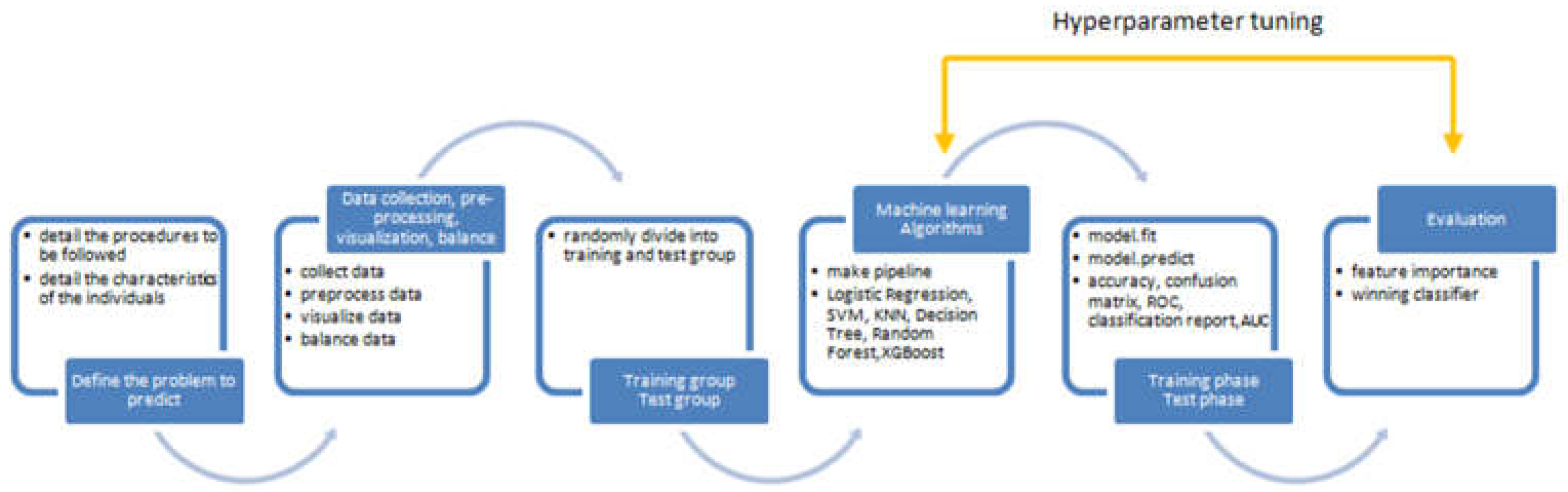
Figure 3.
Unbalanced dataset barplot (regression -92.2%, progression – 7.8%).

Figure 2.
a) bar plot for categorical features versus target; b) box plot for numerical features versus target.
Figure 2.
a) bar plot for categorical features versus target; b) box plot for numerical features versus target.
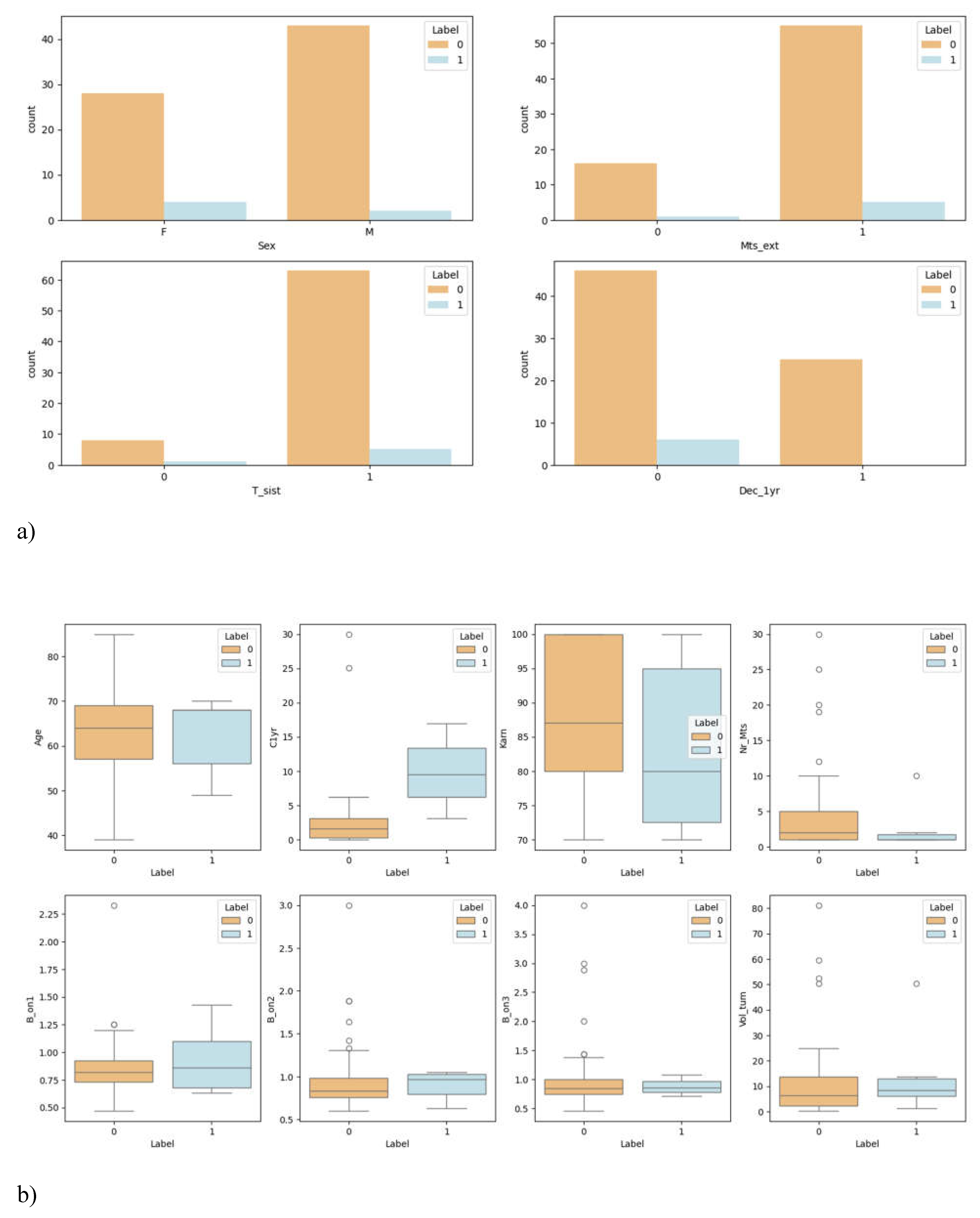
Figure 4.
Confusion matrix for the 6 models tested without tuning.
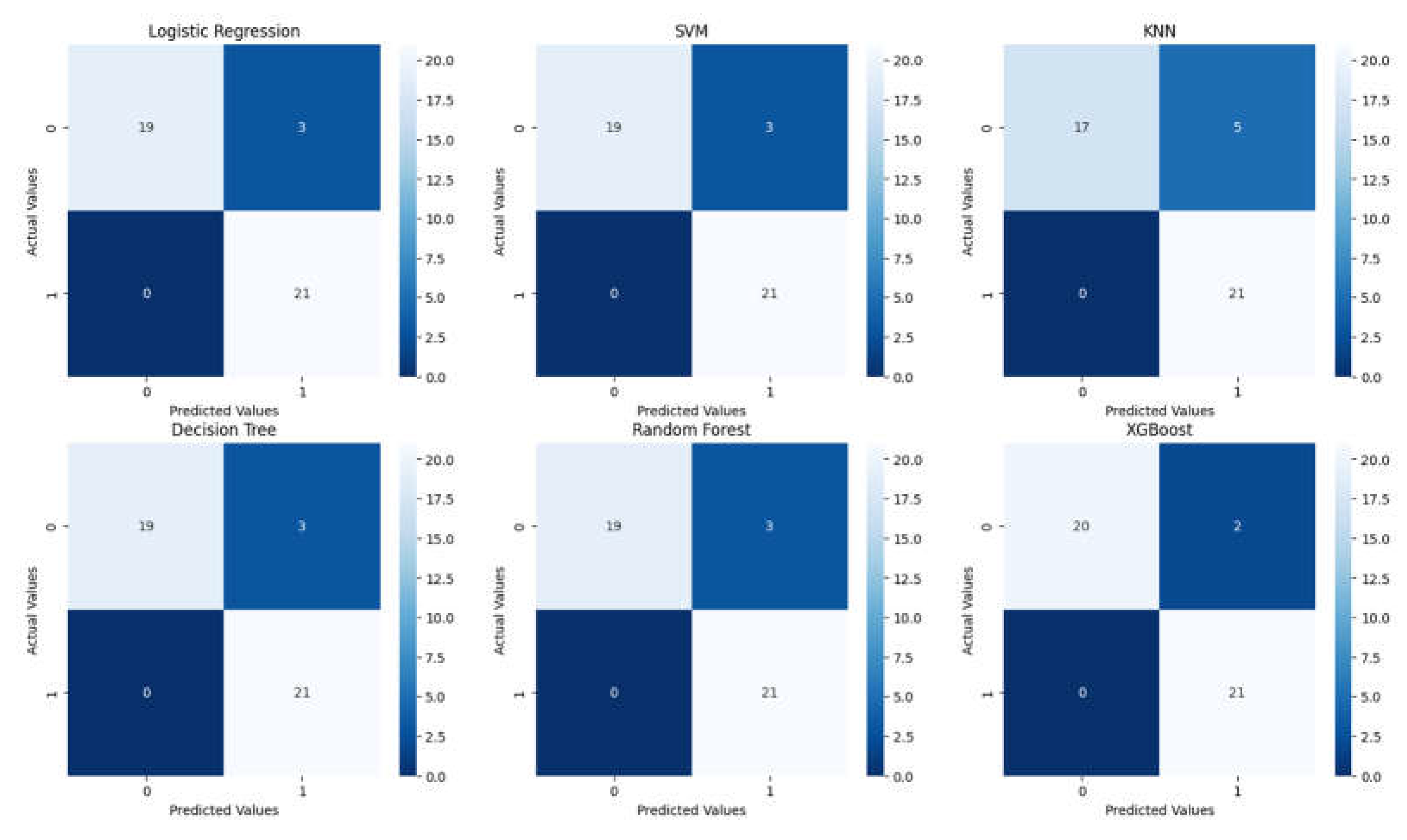
Figure 5.
ROC curves for the 6 models tested without tuning.
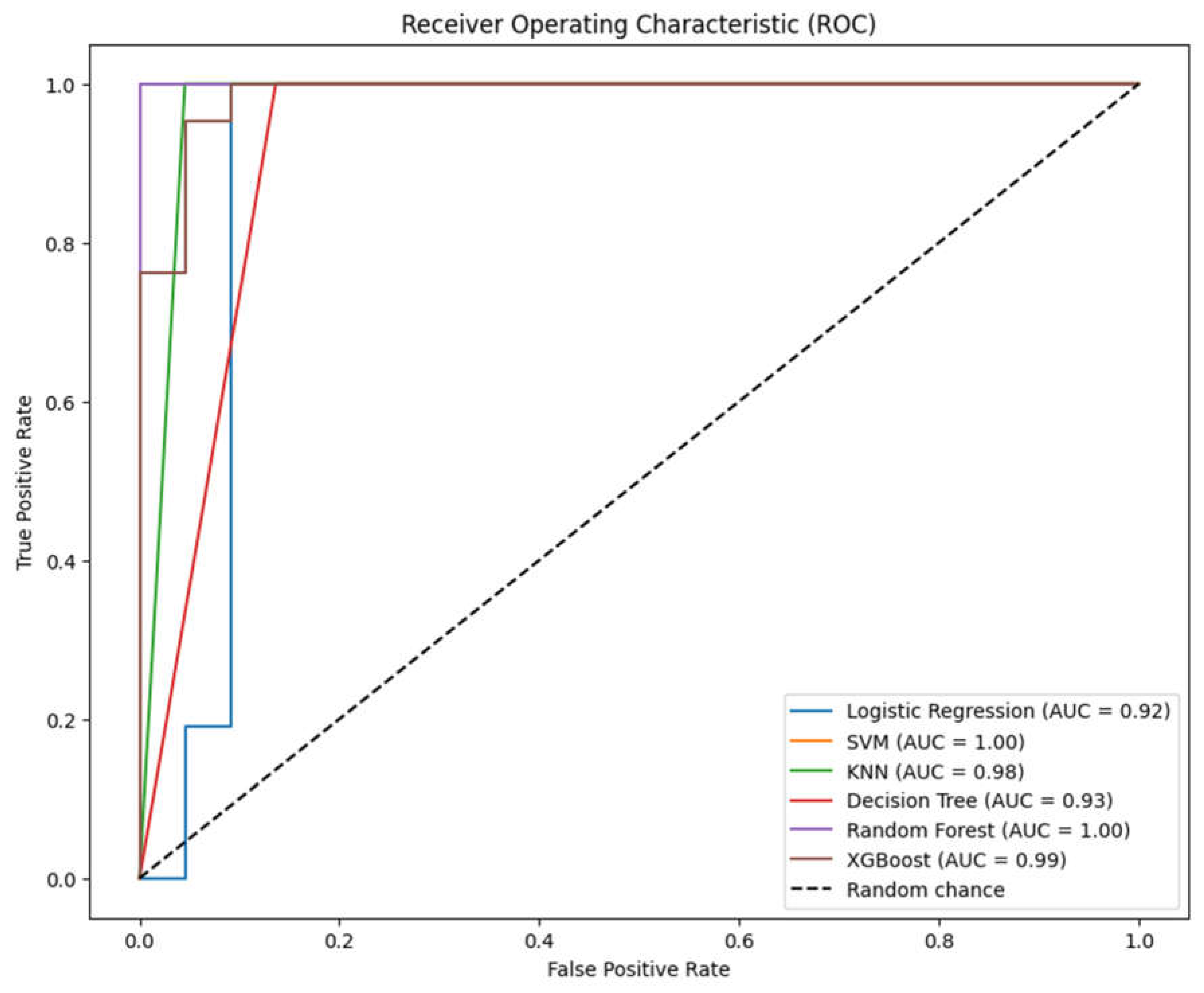
Figure 6.
Confusion matrices for the 6 models tested after tuning.
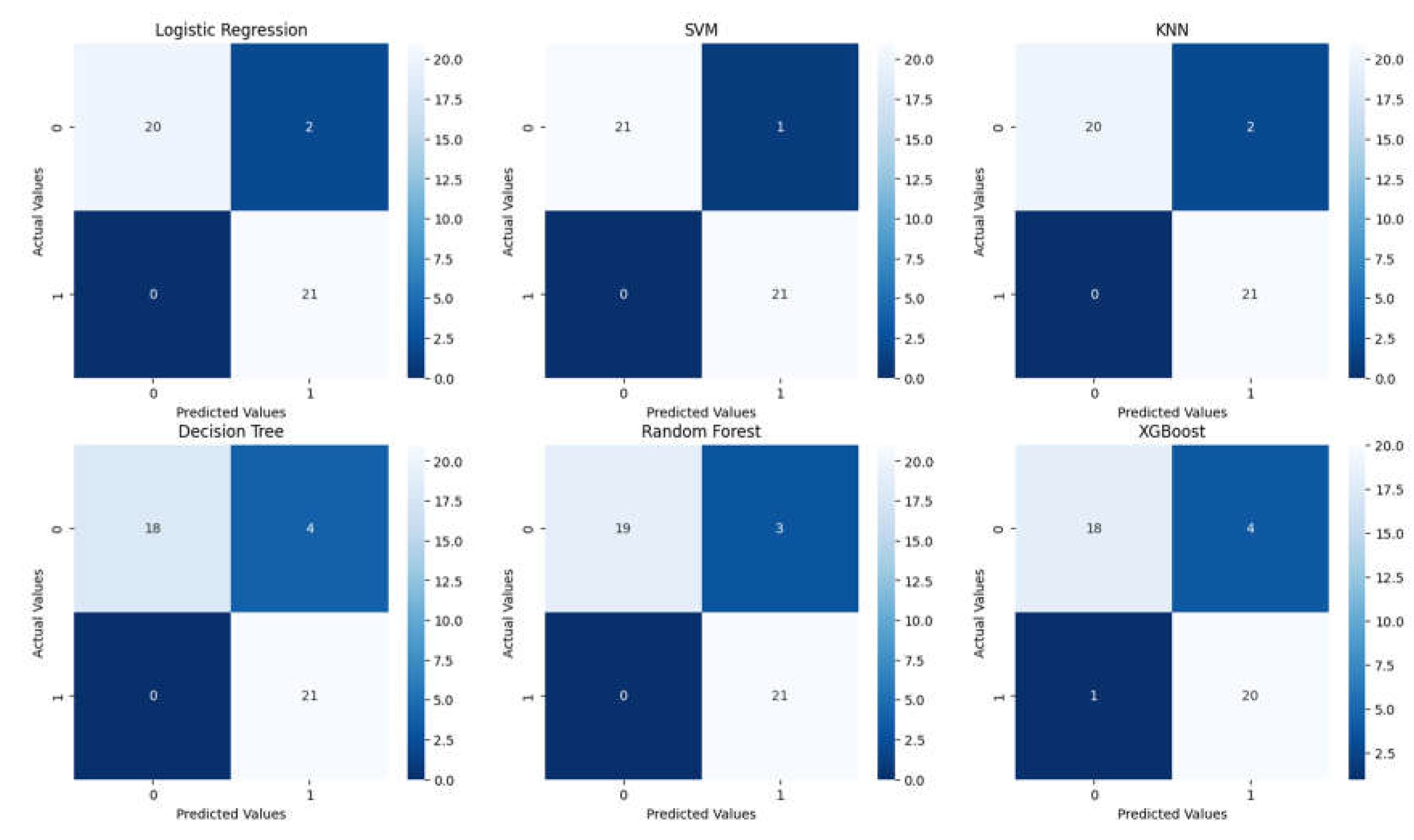
Figure 7.
ROC curves for the 6 models tested after tuning.
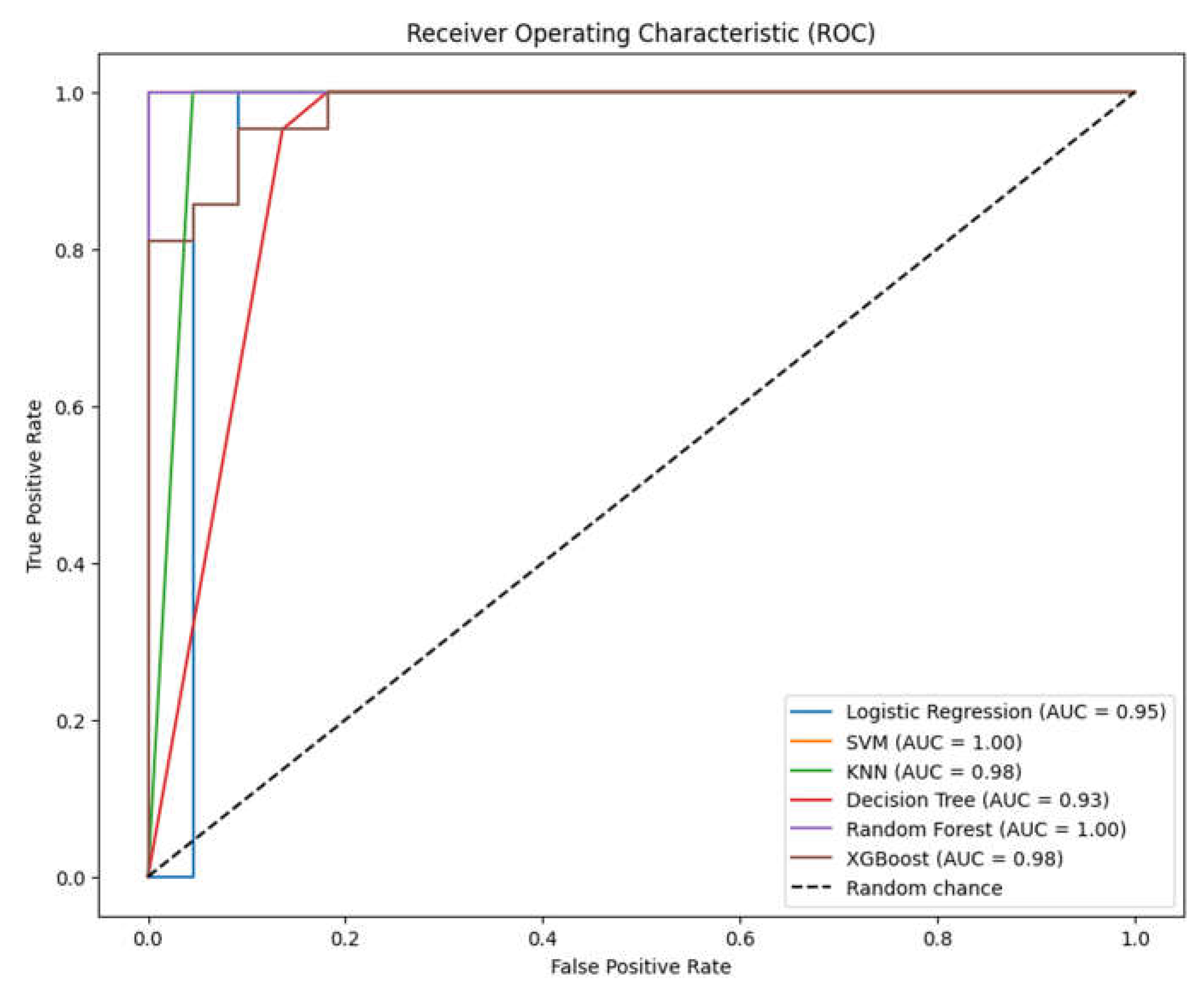
Figure 8.
– feature importance according to Logistic Regression, Decision Tree, Random Forest and XGBoost (no direct feature importance plot available for: SVM, KNN). See Table 2 for feature number correspondences.
Figure 8.
– feature importance according to Logistic Regression, Decision Tree, Random Forest and XGBoost (no direct feature importance plot available for: SVM, KNN). See Table 2 for feature number correspondences.
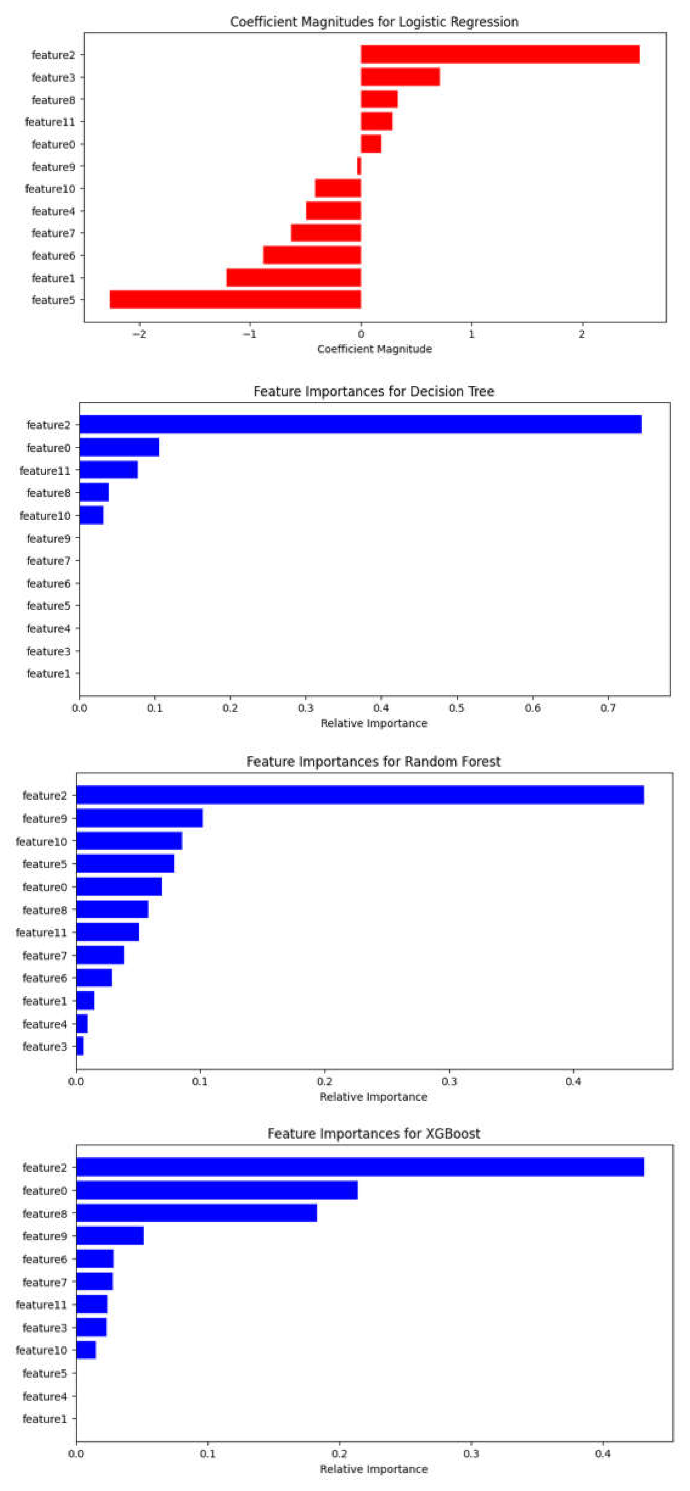

Table 1.
Patient demographics for brain metastases from various primary cancers.
| Characteristics | Value |
|---|---|
| Number of patients | 77 |
| Age(yr) Median (range) |
64(39-85) |
| Sex Male(%) Female(%) |
45(58.44%) 32(41.56%) |
| C1yr – control over one year (cm3) Median(range) |
17 missing data* 0.9(0-30) |
| Patience with extra cranial MTS |
6 missing data* 54 |
| Receiving pre-treatment, systemic treatment | 68 |
| Deceased before 1 year | 1 missing data* 25 |
| KPS score 100 90 80 70 |
9 missing data (11.69%)* 26(33.77%) 8(10.39%) 22(28.57%) 12(15.58%) |
| The number of lesions Median(range) 1-3 4-6 7-10 >10 |
2(1-30) 52 12 8 5 |
| Beam on time on V1 (min/cm3) Median(range) |
0.82(0.47-2.33) |
| Beam on time on V2 (min/cm3) Median(range) |
1 missing data* 0.83(0.60-3.00) |
| Beam on time on V3 (min/cm3) Median(range) |
2 missing data* 0.83(0.46-4.00) |
| Total tumor volume (# of patients with) : < 5 cm3 <= 10 cm3 > 10 cm3 |
34 13 30 |
| Tumor dynamics (# of patients with) : - Progression - Regression |
6 71 |
Table 2.
Summary of features categorized for machine learning algorithms.
| Feature | Feature number |
Description | Categorical/numeric data for machine learning algorithm |
Type |
|---|---|---|---|---|
| Age | 0 | Age at time of treated GKRS | No categorical | Discrete |
| Sex | 1 | Biological sex | 0 = Female; 1 = Male Label encoding |
Numeric |
| C1yr – control over one year | 2 | Volume of lesion measured at the 1 year control | No categorical | Numeric |
| Patience with extra cranial MTS | 3 | Patients having detected with extracranial metastases | 0 = No; 1 = Yes Label encoding |
Numeric |
| Receiving pre-treatment | 4 | Before GKRS, treated by surgery or radiotherapy, or performed chemotherapy | 0 = No pretreatment; 1 = Pretreatment Label encoding |
Numeric |
| Deceased before 1 year | 5 | Patients who passed away before 1 year after receiving GKRS | 0 = Alive; 1 = Deceased Label encoding |
Numeric |
| KPS score | 6 | KPS score runs from 0 to 100. Three physicians allow to evaluate the patient ability to receive GKS for BM. |
No categorical | Numeric |
| The number of lesions | 7 | This divided the 4 groups from the number of lesions. | No categorical | Discrete |
| Beam on time on V1 | 8 | The beam on time on V1 treated over the number of isocenters in V1 | No categorical | Numeric |
| Beam on time on V2 | 9 | The beam on time on V2 treated over the number of isocenters in V2 | No categorical | Numeric |
| Beam on time on V3 | 10 | The beam on time on V3 treated over the number of isocenters in V3 | No categorical | Numeric |
| Total tumor volume | 11 | This divided the 3 groups from the number of volumes. | No categorical | Numeric |
| Tumor dynamics | Label | Tumor progression or regression within 3 months following GKRS treatment. | 0 = Regression; 1 = Progression |
Discrete |
Table 3.
Accuracy, AUC for the 6 models tested without tuning.
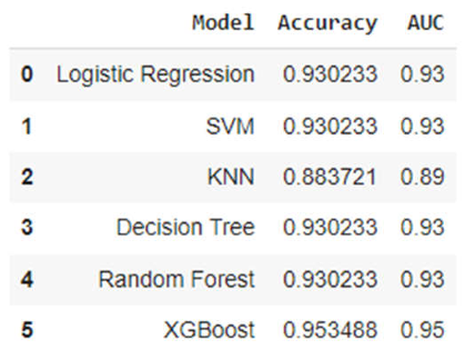
Table 4.
Classification report for the 6 models tested without tuning.
| Classification Report for Logistic Regression | ||||
| precision | recall | F1-score | Support | |
| 0 | 1.0 | 0.86 | 0.93 | 22 |
| 1 | 0.88 | 1.00 | 0.93 | 21 |
| accuracy | 0.93 | 43 | ||
| macro avg | 0.94 | 0.93 | 0.93 | 43 |
| weighted avg | 0.94 | 0.93 | 0.93 | 43 |
| Classification Report for SVM | ||||
| precision | recall | F1-score | Support | |
| 0 | 1.0 | 0.86 | 0.93 | 22 |
| 1 | 0.88 | 1.00 | 0.93 | 21 |
| accuracy | 0.93 | 43 | ||
| macro avg | 0.94 | 0.93 | 0.93 | 43 |
| weighted avg | 0.94 | 0.93 | 0.93 | 43 |
| Classification Report for KNN | ||||
| precision | recall | F1-score | Support | |
| 0 | 1.0 | 0.77 | 0.87 | 22 |
| 1 | 0.81 | 1.00 | 0.89 | 21 |
| accuracy | 0.88 | 43 | ||
| macro avg | 0.90 | 0.89 | 0.88 | 43 |
| weighted avg | 0.91 | 0.88 | 0.88 | 43 |
| Classification Report for Decision Tree | ||||
| precision | recall | F1-score | Support | |
| 0 | 1.0 | 0.86 | 0.93 | 22 |
| 1 | 0.88 | 1.00 | 0.93 | 21 |
| accuracy | 0.93 | 43 | ||
| macro avg | 0.94 | 0.93 | 0.93 | 43 |
| weighted avg | 0.94 | 0.93 | 0.93 | 43 |
| Classification Report for Random Forest | ||||
| precision | recall | F1-score | Support | |
| 0 | 1.0 | 0.86 | 0.93 | 22 |
| 1 | 0.88 | 1.00 | 0.93 | 21 |
| accuracy | 0.93 | 43 | ||
| macro avg | 0.94 | 0.93 | 0.93 | 43 |
| weighted avg | 0.94 | 0.93 | 0.93 | 43 |
| Classification Report for XGBoost | ||||
| precision | recall | F1-score | Support | |
| 0 | 1.0 | 0.91 | 0.95 | 22 |
| 1 | 0.91 | 1.00 | 0.95 | 21 |
| accuracy | 0.95 | 43 | ||
| macro avg | 0.96 | 0.95 | 0.95 | 43 |
| weighted avg | 0.96 | 0.95 | 0.95 | 43 |
Table 5.
Accuracy and AUC for the 6 models tested after tuning.
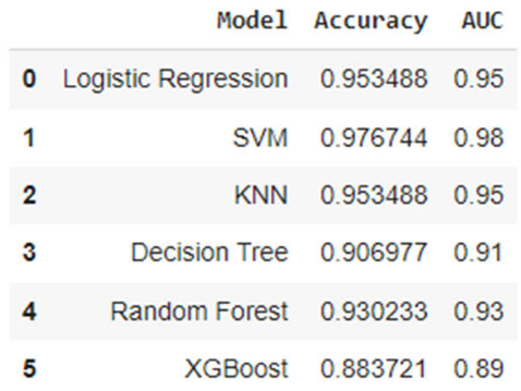
Table 6.
Classification report for the 6 models tested after tuning.
| Classification Report for Logistic Regression | ||||
| precision | recall | F1-score | Support | |
| 0 | 1.0 | 0.91 | 0.95 | 22 |
| 1 | 0.91 | 1.00 | 0.95 | 21 |
| accuracy | 0.95 | 43 | ||
| macro avg | 0.96 | 0.95 | 0.95 | 43 |
| weighted avg | 0.96 | 0.95 | 0.95 | 43 |
| Classification Report for SVM | ||||
| precision | recall | F1-score | Support | |
| 0 | 1.0 | 0.95 | 0.98 | 22 |
| 1 | 0.95 | 1.00 | 0.98 | 21 |
| accuracy | 0.98 | 43 | ||
| macro avg | 0.98 | 0.98 | 0.98 | 43 |
| weighted avg | 0.98 | 0.98 | 0.98 | 43 |
| Classification Report for KNN | ||||
| precision | recall | F1-score | Support | |
| 0 | 1.0 | 0.91 | 0.95 | 22 |
| 1 | 0.91 | 1.00 | 0.95 | 21 |
| accuracy | 0.95 | 43 | ||
| macro avg | 0.96 | 0.95 | 0.95 | 43 |
| weighted avg | 0.96 | 0.95 | 0.95 | 43 |
| Classification Report for Decision Tree | ||||
| precision | recall | F1-score | Support | |
| 0 | 1.0 | 0.82 | 0.90 | 22 |
| 1 | 0.84 | 1.00 | 0.91 | 21 |
| accuracy | 0.91 | 43 | ||
| macro avg | 0.92 | 0.91 | 0.91 | 43 |
| weighted avg | 0.92 | 0.91 | 0.91 | 43 |
| Classification Report for Random Forest | ||||
| precision | recall | F1-score | Support | |
| 0 | 1.0 | 0.91 | 0.95 | 22 |
| 1 | 0.91 | 1.00 | 0.95 | 21 |
| accuracy | 0.95 | 43 | ||
| macro avg | 0.96 | 0.95 | 0.95 | 43 |
| weighted avg | 0.96 | 0.95 | 0.95 | 43 |
| Classification Report for XGBoost | ||||
| precision | recall | F1-score | Support | |
| 0 | 0.95 | 0.82 | 0.88 | 22 |
| 1 | 0.83 | 0.95 | 0.89 | 21 |
| accuracy | 0.88 | 43 | ||
| macro avg | 0.89 | 0.89 | 0.88 | 43 |
| weighted avg | 0.89 | 0.88 | 0.88 | 43 |
Disclaimer/Publisher’s Note: The statements, opinions and data contained in all publications are solely those of the individual author(s) and contributor(s) and not of MDPI and/or the editor(s). MDPI and/or the editor(s) disclaim responsibility for any injury to people or property resulting from any ideas, methods, instructions or products referred to in the content. |
© 2024 by the authors. Licensee MDPI, Basel, Switzerland. This article is an open access article distributed under the terms and conditions of the Creative Commons Attribution (CC BY) license (http://creativecommons.org/licenses/by/4.0/).
Copyright: This open access article is published under a Creative Commons CC BY 4.0 license, which permit the free download, distribution, and reuse, provided that the author and preprint are cited in any reuse.


