
Submitted:
30 April 2024
Posted:
30 April 2024
You are already at the latest version
Abstract
Timber-concrete composite (TCC) systems join the positive aspects of engineered wood products (good seismic behaviour, low thermal conductivity, environmental sustainability, good behaviour under fire if appropriately designed) with those of concrete (high thermal inertia, durability, excellent fire resistance). TCC facades are typically composed by an internal insulated timber-frame wall and an external concrete slab, separated by a ventilated air cavity. However, there is very limited knowledge concerning the performance of TCC facades, especially for what concerns their thermal behaviour. The present paper deals with the development and optimisation of a 2D CFD model for the analysis of TCC ventilated façades thermal behaviour. The model is calibrated and validated against the experimental data collected during the annual monitoring of a real TCC ventilated envelope in the north of Italy. Also, a new solver algorithm is developed to significantly speed up the simulation. The final model can be used for the time-efficient analysis and optimisation of the thermal performance of TCC ventilated facades, as well as other ventilated facades with external massive cladding, avoiding the expensive and time-consuming construction of mock-ups, or the use of comparably slow (conventional) CFD solvers that are less suitable for optimization studies.
Keywords:
ventilated façade
; CFD
; timber-concrete composite façade
; timber-based construction
; thermal performance.
1. Introduction
In recent years, the building sector has been characterized by the rapid growth in the use of engineered wood products (EWPs) thanks to the great properties related to seismic behaviour, thermal insulation, environmental sustainability, the good behaviour under fire (if designed in appropriate way), the strong attitude towards prefabrication and systems integration, and the possibility of disassembly at the end of life [1]. But EWPs are also characterized by a fragile stress-strain behaviour, high hygroscopicity and low durability if not properly protected [2]. Speaking about envelopes, lightweight timber facades have low thermal inertia and poor acoustic performance if compared to alternatives with higher mass, while massive timber solutions involve a significant consumption of virgin material and have high costs. To overcome some of the material limits and achieve an improved behaviour in terms of mechanical properties, acoustic performance, fire resistance and durability, timber structures are sometimes integrated with concrete, resulting in timber-concrete composite (TCC) systems [3].
TCC facades are usually composed by an internal highly insulated timber wall coupled with an external massive concrete slab acting as shield against the weather agents [4], also in case of extreme weather events like windstorms and hailstorms. Such composite facades join the positive aspects of EWPs (reduced weight, good thermal insulation, sustainability, ease of prefabrication and systems integration, nice aesthetics, etc.) with those of concrete (good mechanical resistance, high thermal inertia, good acoustic insulation, excellent durability, fire resistance, etc.) [5]. Also, they can lead to innovative aesthetic solutions for off-site timber-based construction since the presence of a concrete slab allows the application of heavy materials (e.g. stone slabs) or the reproduction of 2D/3D patterns and textures as external finishing.
Besides off-site timber-based construction, nowadays another widely discussed topic concerns the use of ventilated façades and their advantages in terms of thermal, acoustic, and water-tightness properties [6]. TCC facades can also be ventilated facades. In this case, the presence of an air cavity between the timber wall and the concrete slab is also useful for the separation between the external (potentially humid) concrete slab, acting as weather protection, and the internal timber insulated wall, that must be always dry. Several research studies in literature highlight the good thermal behaviour of ventilated facades during summer, thanks to the chimney effect in the cavity [6,7,8]. The detailed assessment of the energy performance of ventilated façades is a constantly current issue in research since their interaction with the external environment is complex and requires experimental tests and CFD analysis of the air flow inside the cavity [9]. Considering ventilated facades with external massive cladding, very little research is present in literature [6] and no study about their CFD modelling was found. Thus, further research on the thermal behaviour of TCC ventilated façades is needed.
CFD is an extremely valuable tool for performance analysis: Pastori et al. [4] demonstrated that such simulations can highlight the limitations of the current Standards in predicting ventilated facades thermal performance. However, in their study the solid layers of the studied envelope were simplified by adopting a 1D approach (an experimental validation was not followed), leading to a single-region simulation. The same approach was followed by other studies in the field [10]. More recent work performed the so-called “conjugate heat transfer” (CHT)-based simulations, where also the temperature distribution in all solids is computed co-currently with the flow problem (multi-region simulation). Examples of such studies in the field of indoor room flow include the early work of Horikiri et al. [11]. However, for the study of ventilated façades, single-region simulations dominate, making the applied boundary conditions the critical factor [9]. One of the few exceptions is the study of Brandl et al. [12], which considered multiple solid regions in the simulation. However, in this case, several material parameters (e.g. heat conductivity or emissivity, important for radiation effects) must be chosen. To overcome the problem of unknown parameters, calibration must be used, as done by Fantucci et al. [13], although based on a simple flow model. Also, transient multi-region simulations are considerably more computationally expensive, since the region with the largest thermal relaxation time (i.e. with the slowest thermal response) dictates the number of time steps to be performed. Potential solutions to such a strategy are parallelization, implicit thermal coupling [14], or the simplification of the regions (usually the solid regions; sometimes simply the grid resolution is reduced).
1.1. Objectives
The central goal of the research was to establish a comprehensive multi-region CFD model to describe the thermal performance of TCC ventilated façades. Specifically, the first sub-goal was to implement the model and a novel algorithm for time stepping in the well-known CFD solver OpenFOAM (OpenFOAM® v2206 was used, see Appendix A for details). Similarly to Laitinen et al. [15] and Chourdakis et al. [14], the solver “chtMultiRegionFoam” was used as the basis for the work. The second sub-goal was to perform a sensitivity analysis of the model prediction with respect to key input parameters (i.e. the physical properties and boundary conditions applied). The final goal was the calibration of a key parameter (i.e., the heat capacity of the solid region), and the validation of the predictive capability of the calibrated and non-calibrated model.
2. Materials and Methods
The research focuses on the study of the thermal behaviour of the TCC prefabricated ventilated façade system in Figure 1. The system is composed of an internal timber-frame structure coupled with an external 50 mm thick reinforced concrete slab, separated by independent vertical ventilated air cavities. The external cladding (the concrete slab) has sealed joints, which means that each air cavity is connected to the external environment only at the bottom and top of the façade, whose height depends on the building elevation and on the presence of windows and/or protruding slabs. The TCC façade analysed is part of the envelope of a residential 3-storey building located in the north of Italy, close to Brescia (Figure 2). In this case, the ventilated façade height is equal to two storeys of the building (the ground floor has a different envelope system), which is the minimum height that allows to gain some benefits from the natural ventilation inside the cavity of the façade, according to literature. The thermal behaviour of the façade indicated in Figure 2 was monitored over one year, from August 2022 until August 2023, [16] and the results used to calibrate and validate the CFD model described in this paper.
2.1. Geometry of the Model
A two-dimensional model was developed to study the façade behaviour (Error! Reference source not found.). This choice was due to the need of keeping the model as simple as possible, and it was compatible with the geometry of the façade. In fact, since the air flows through many independent cavities, characterized by limited width (80 cm), horizontal air flows are negligible. For this reason, a 2D façade model, which neglects the third spatial dimension, was adequate for the study purpose.
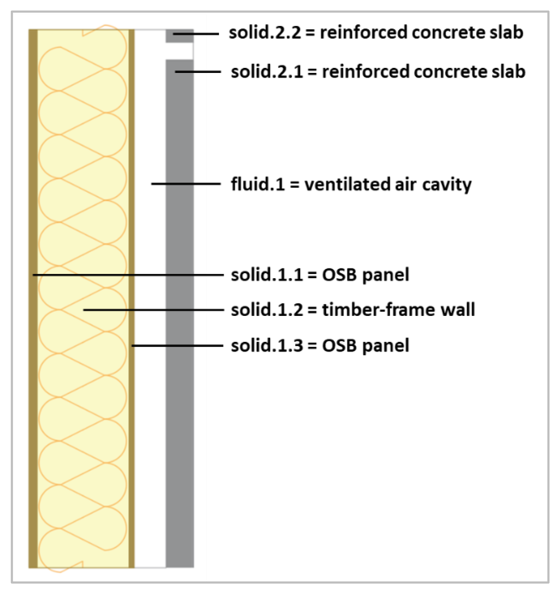
Figure 3.
Regions (solid and fluid) of the CFD model.
2.2. Physical Properties of the Model
The thermo-physical properties assigned to each material (i.e. each region) of the CFD model are reported in Table 1.
2.3. Boundary Conditions
The boundary conditions applied to the model are described in this paragraph. Figure 4 shows the main boundary conditions applied to the CFD model. The trends of the variables T_air,i (indoor air temperature), T_air,e (outdoor air temperature), qr_incident (solar irradiation incident on the facade), V_air,e (air velocity at the bottom inlet of the cavity) were taken from the experimental monitoring; the values of hi (convective-radiative coefficient of indoor environment), he (convective-radiative coefficient of outdoor environment), Rse (surface resistance of outdoor environment) were taken from the Standard ISO 6946 [17]; the values of T_outlet (air temperature at the top outlet of the cavity), P_outlet (air pressure at the top outlet of the cavity), V_outlet (air velocity at the top outlet of the cavity) are calculated by the software during the simulation. The complete setting of boundary conditions is reported in Appendix A.
2.4. Mesh Refinement Study
A mesh refinement study was performed, to identify the best model discretization in terms of accuracy of the results and computational cost. Three meshes were tested by setting a simple simulation case:
- m0012_baseMesh
- m0013_baseMeshx1.5
- m0014_baseMeshx1.5x1.5
The number of cells for each mesh was equal to the number of the previous one multiplied for 1.5 in both vertical and horizontal directions. As expected, the results obtained showed that the grid refinement produces a slightly better accuracy, but with higher computational time. In this specific case, the improvement of the mesh accuracy did not produce consistent differences in the results, while the time needed for the computation increased considerably (see Table 2). For this reason, m0012 was chosen and used for all the future simulations. The geometry and mesh used are shown in Figure 5.
The first simulation (t0001) was run for 96 hours (4 days), to see how long the model needed for catching the right temperature trends. The results of the first simulation showed that 48 hours were enough for that, thus the second case (t0002) was run for 48 hours. The third simulation (t0003) was stopped after 24 hours because of the huge amount of time needed.
2.5. Solver
The solver used (chtMultiRegionFoamIPPT, see Appendix A for details of the source code) allows to couple a transient fluid flow with heat transfer between regions, buoyancy effects, turbulence, and radiation modelling. The solver follows a segregated solution strategy, which means that the equations for each variable characterizing the system are solved sequentially and the solution of the preceding equations is inserted in the subsequent equation. The coupling between fluid and solid follows the same strategy: first the equations for the fluid are solved using the temperature of the solid of the preceding iteration to define the boundary conditions for the temperature in the fluid. After that, the equation for the solid is solved using the temperature of the fluid of the preceding iteration to define the boundary condition for the solid temperature. This iteration procedure is executed until convergence. For each fluid region the compressible Navier Stokes equation is solved, while for the solid regions only the energy equation has to be solved. The regions are coupled by a thermal boundary condition.
2.5.1. A New “Frozen-Unfrozen Flow” Solver
A novel algorithm, called the “frozen-unfrozen flow” solver, was developed to speed up the simulations, and consequently the overall model calibration process. The new solver features are explained in the following paragraph.
The purpose of developing this new solver was simply to speed up the simulation by switching the solution mode to “frozen” (i.e. no update of the velocity and pressure field, allowing large time steps) and “unfrozen” (i.e. solution of all transport equations, with normal time steps) sequentially. The normal time step in the “unfrozen” mode is determined by the Courant number and the solid diffusion numbers, while the time stepping in the “frozen” mode is set based on user input.
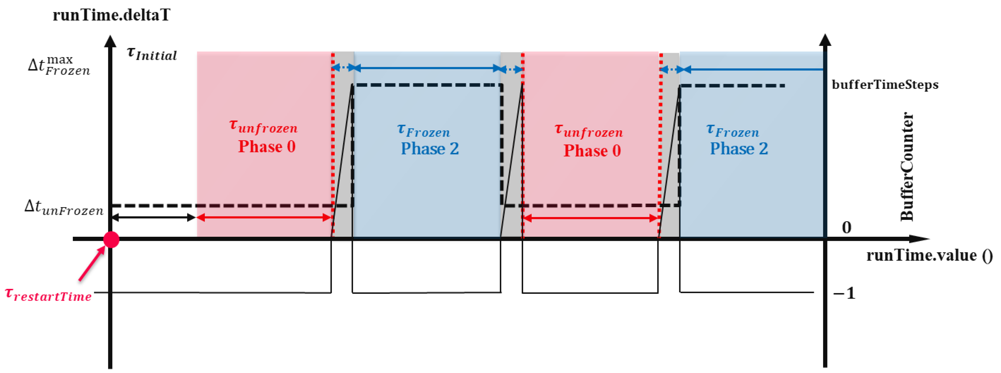
Error! Reference source not found. shows the schematic view of this algorithm. It starts with the initial time ( and then several cycles with unfrozen (red zones) and frozen (blue zones) are repeated till the end of the simulation. For stability reasons, a transition mode (the grey zones) must be also considered when the flow mode is switched between “frozen” and “unfrozen”.
To do so, two periods were considered:
- “initial period”, when the fluid flow evolves according to time steps calculated based on Courant and solid diffusion numbers, to make the simulation stable at the beginning. It should be noted that the initial time not necessarily starts at time 0, since the algorithm is designed to work also in the case the simulation is re-started;
- “normal period”: in which the flow is sequentially set to frozen and unfrozen modes.
Algorithmic details related to these periods are summarized in Appendix B for the interested reader.
Figure 6.
Illustration of the new solver algorithm by considering an “initial period”, and the “normal period” consisting of a “frozen” and “unfrozen” phase.
Figure 6.
Illustration of the new solver algorithm by considering an “initial period”, and the “normal period” consisting of a “frozen” and “unfrozen” phase.
2.5.2. Solver Performance Evaluation
To test the new solver performance, new cases were created varying τfrozen and τunfrozen in a systematic way to explore the effect of these numerical parameters on the accuracy of the results (i.e. the temperature values obtained in the model) and the time needed for the computation. The new cases were compared to a base case, t0001, identical to the new ones, but run with the old solver. Table 3 resumes the results obtained from the new cases.
All the simulations were run for 24 hours real time. and were set equal to 1s. The relative performance of the code, compared to the theoretical maximum performance that can be reached with the freeze/unfreeze setting used, was calculated as:
Relative performance = simulation speedup/(1+τfrozen /τunfrozen)
As expected, the simulation speed increased by increasing the ratio τfrozen /τunfrozen, while the accuracy did not seem to be inversely proportional to the speed. The relative performance of the code shows how close the speed increase was to the theoretical optimum. For example, for case t0011, the new algorithm reaches almost the maximum performance of the code (i.e., 90% of the theoretical optimum). Instead, for case t0016, the relative performance was only at 45%, indicating a potential to further increase the observed speedup of x45.
2.6. Model Calibration
First of all, a sensitivity analysis was developed by comparing the results from the CFD model with the experimental data obtained. It consisted in changing the physical and numerical parameters used in the modelling to fit the CFD results to the experimental ones. The experimental data regarding the thermal behaviour of the façade during summer sunny days (from the 23rd to the 25th of August 2022) was used as benchmark for the comparison. The overview of the simulations run for calibration is reported in Table 4. To run the cases the old solver was used, since the new one was still under development.
After the sensitivity analysis, the case that produced the lowest error in the results was considered as starting point for the calibration process. The calibration consisted in changing systematically one parameter of the model and see how this change affected the final results.
2.7. Model Validation
The validation process is necessary to test whether the model works also for different boundary conditions. After the calibration of the CFD model against the experimental results collected for summer sunny days, the model was tested again considering summer cloudy days (from the 18th to the 20th of August 2022).
3. Results
In this chapter, the results obtained with the CFD model are presented and analysed. The temperatures measured on the different surfaces of the facade are identified using the following codes:
- TR: average temperature on the internal surface of the indoor OSB panel;
- TO: average temperature on the surface towards the cavity of the outdoor OSB panel;
- TC: average temperature on the concrete slab surface towards the ventilated cavity;
- TC_ext: average temperature on the external surface of the concrete slab.
Also, the results of the sensitivity analysis and of the calibration process are discussed. Ultimately, a comparison between the results obtained from the experimental monitoring and those given by the calibrated model is presented.
3.1. Sensitivity Analysis
Table 5 contains the results of the sensitivity analysis. The errors were calculated considering only the last 24h simulated, to exclude the transient part at the beginning of the simulations. Temperature TR is not reported in Table 5 since its values are predicted very well by the CFD model in all the cases run, with an error lower than 1% between the experimental values and the simulations.
3.2. Calibration Process
Starting from simulation t0104, the specific heat capacity (cp) of solid.2 (concrete) was systematically changed to find the optimum value that allowed to minimize the error between the experimental value and the CFD prediction of temperature TO. Simulation t0104 was chosen because it is one of the cases with lower average error and lower error in TO (see Table 5). Temperature TO was used as reference because, together with TR, it determines the heat flux entering the building through the timber-frame wall. As already mentioned, temperature TR is always well predicted by the CFD model in all the cases run during the sensitivity analysis. The results from the calibration are shown in Table 6 and Error! Reference source not found..
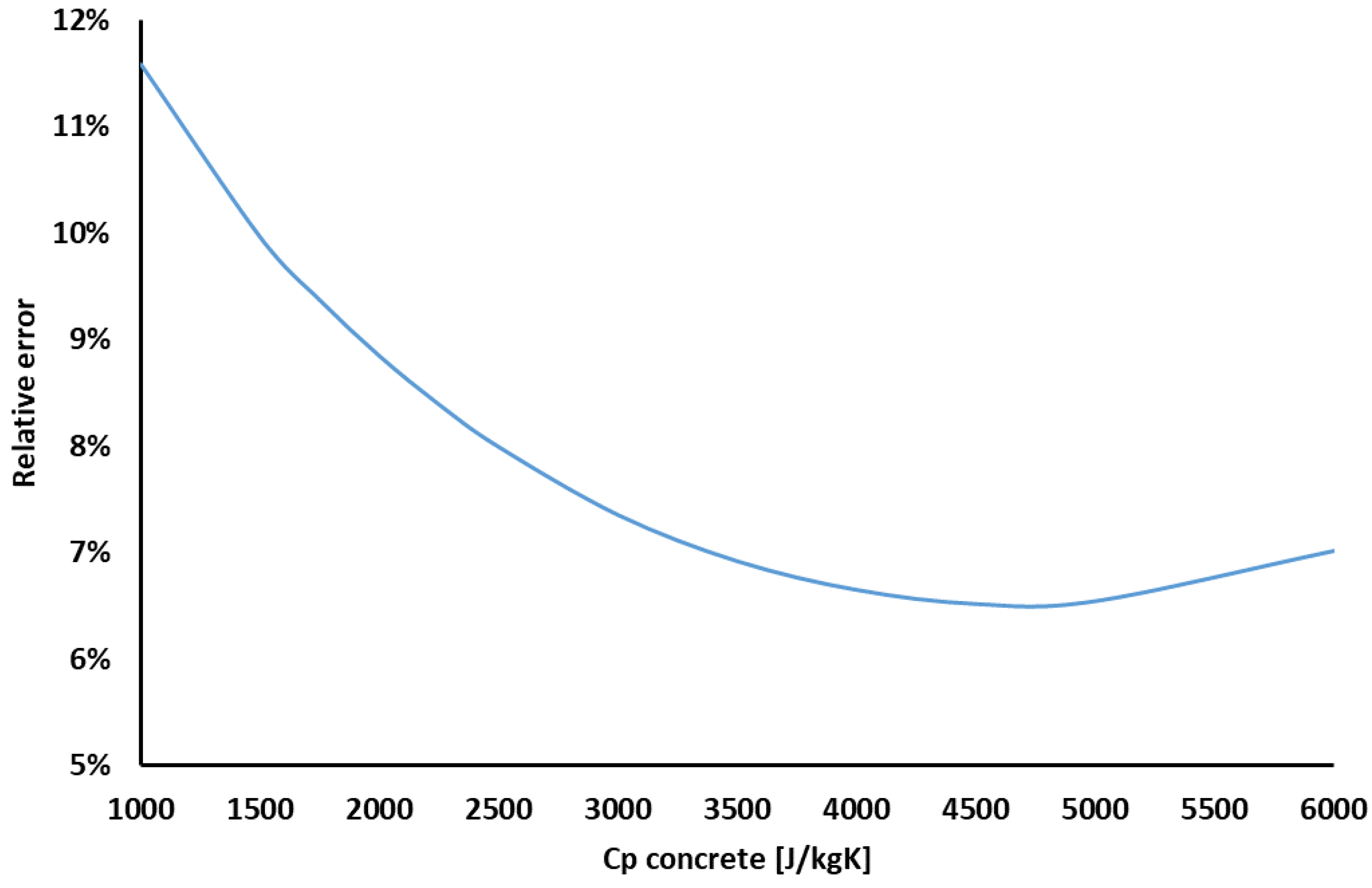
According to the model, the lowest error in the temperature TO is 6.5% and corresponds to case t4500, which considered a Cp for concrete equal to 4500 J/kgK, i.e. 4.5 times higher than the reference value prescribed by the Standard EN ISO 10456 [17]. This result is unrealistic and probably affected by a CFD model issue that leads to low temperatures prediction into the cavity (documented in paragraph 4.3).

Table 6.
Steps and results of calibration process.
| Results of calibration process | ||||
| Case | Description | Cp_concrete (J/kgK) |
Error of TO prediction |
Note |
| t1000 (= t0101) | 1xCp_concrete_base | 1000 | 11.59% | Cp value from EN ISO 10456:2007 |
| t1500 | 1.5xCp_concrete_base | 1500 | 9.97% | |
| t1750 | 1.75xCp_concrete_base | 1750 | 9.38% | |
| t2000 (= t0104) | 2xCp_concrete_base | 2000 | 8.85% | starting case |
| t2250 | 2.25xCp_concrete_base | 2250 | 8.40% | |
| t2500 | 2.5xCp_concrete_base | 2500 | 8.00% | |
| t3000 | 3xCp_concrete_base | 3000 | 7.36% | |
| t3500 | 3.5xCp_concrete_base | 3500 | 6.93% | |
| t4000 | 4xCp_concrete_base | 4000 | 6.66% | |
| t4500 | 4.5xCp_concrete_base | 4500 | 6.52% | best prediction |
| t5000 | 5xCp_concrete_base | 5000 | 6.55% | |
| t6000 | 6xCp_concrete_base | 6000 | 7.02% | |
Figure 7.
Graphical representation of the values listed in Table 6. According to the model, the minimum error is around 6.5% and corresponds to a Cp value of 4500 J/kgK for the concrete.
Figure 7.
Graphical representation of the values listed in Table 6. According to the model, the minimum error is around 6.5% and corresponds to a Cp value of 4500 J/kgK for the concrete.
3.3. Validation Study
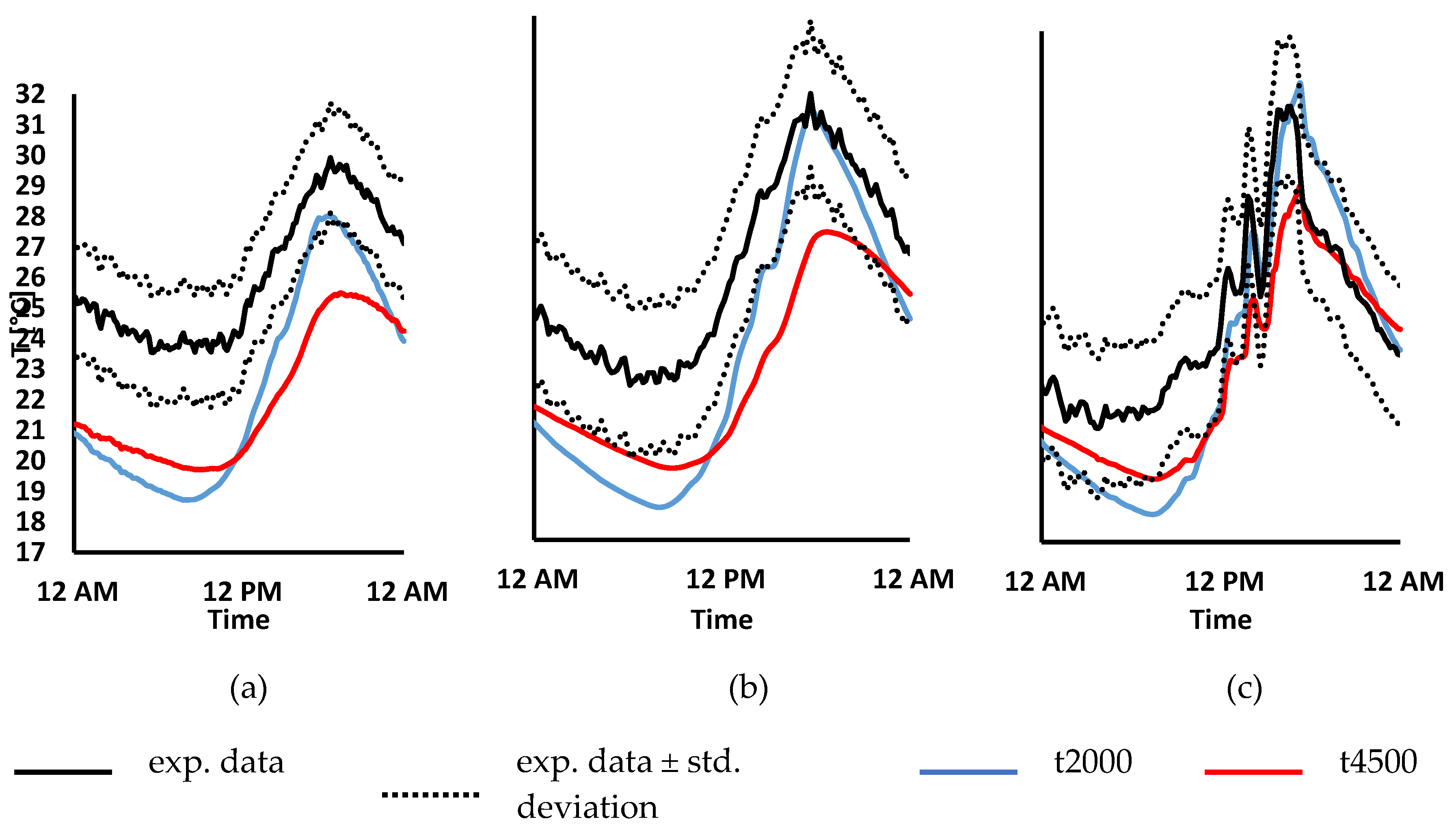
For the validation process, case t2000 (the best case from the sensitivity analysis) and t4500 (the calibrated model) were used, to highlight if the latter was more accurate than the former. The boundary conditions considered in this case refer to summer cloudy days, instead of summer sunny days. The models were run for 48 hours; the average errors of the temperature prediction reported in Table 7 are calculated considering only the last 24 hours, to exclude initialization errors. By looking at the results in Table 7, in general model t0321 predicts with lower error than the calibrated model t4500. However, the trend of model t4500 is more similar to the experimental one (Error! Reference source not found.): if one would consider an offset of approximately 4 °C for TO and TC, the experimental and simulated data would almost perfectly overlap. Similarly, an offset of approximately 1°C for TC_ext would greatly reduce the error.
Figure 8.
Prediction of a) TO, b) TC, and c) TC_ext by model t2000 and t4500.
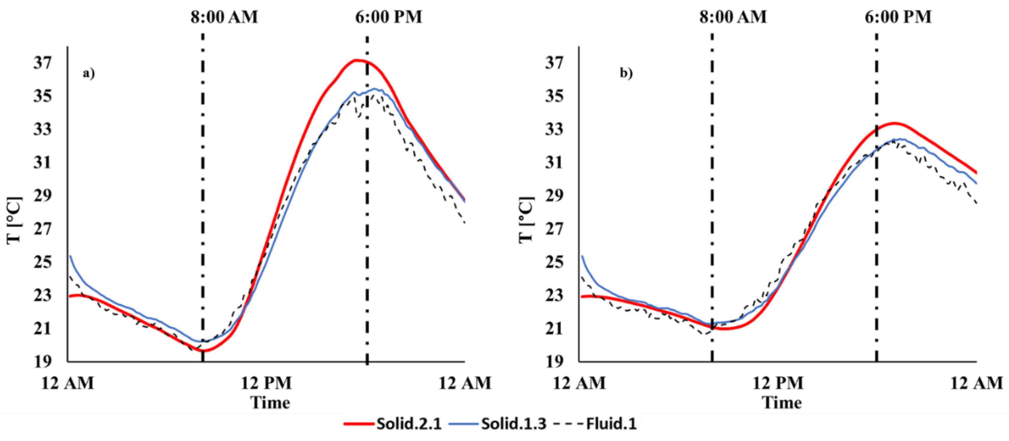
3.4. Discussion of Persistent Underprediction of Surface Temperatures Inside the Cavity
The persistent underprediction of the surface temperatures inside the cavity by the CFD simulation is speculated to be mainly caused by an under resolved flow: specifically, we have assumed a laminar flow in the cavity, but used a relatively coarse computational mesh. Consequently, an instability that might develop in the flow, and increase flow resistance as well as the heat transfer rates were - most likely - not captured in our simulations. Thus, heat transfer from the concrete to the timber wall (specifically its surface) during heat up (noon and early afternoon) is strongly underpredicted. During the cool-off phase (late afternoon) this leads to significantly lower temperatures of the wall cavities, especially the one on the timber side.
3.4.1. Relative Importance of Radiative Heat Transfer Inside the Cavity
The transferred heat flux inside the cavity can be estimated via:
where
Equation (3) is taken from [19].
The cavity is modeled as a 2D domain with a depth of 3 cm. Hence, the heat transfer coefficient for the cavity is calculated as follows if a fixed temperature at the walls is considered:
Now, we need to compute the average temperature of the cavity walls and air in the cavity. These values have been obtained from t0104 and t4500 cases (see Error! Reference source not found.). For an estimate of the patch-averaged heat fluxes due to heat transfer, we picked two time-snapshots on this plot (i.e. 8:00 am and 6:00 pm). We note in passing that the averaged values have been obtained by the “integrate variables” feature in ParaView, which performs an area-weighted calculation. As can be seen in Table 8, the patch-average radiative and transferred heat flux are of similar magnitude. This indicated that both the emissivity of the wall and the details of the flow in the cavity are important when predicting the heat fluxes, and consequently the surface temperatures in the cavity. It should be noted that a negative radiative heat flux (i.e. ) means that radiative heat leaves the patch.
Figure 9.
Volume averaged temperature of fluid.1 as well as the patch averaged temperature of solid2.1 and solid.1.3 in contact with fluid.1 as a function of time case for case t0104 (left panel), and case t4500 (right panel).
Figure 9.
Volume averaged temperature of fluid.1 as well as the patch averaged temperature of solid2.1 and solid.1.3 in contact with fluid.1 as a function of time case for case t0104 (left panel), and case t4500 (right panel).
4. Conclusions
Starting from data collected during an annual experimental campaign in the north of Italy, close to Brescia (described in [16]) the present paper focuses on the description and optimisation of a multi-region CFD model. The experimental campaign was conducted on a TCC ventilated façade, part of a real building envelope, over one year. The experimental data collected were used for the calibration and validation of a 2D CFD model, that was developed and optimised for the specific envelope system but might also be used for different types of ventilated facades composed by an internal lightweight wall and an external massive cladding. Several CFD models for the thermal analysis of ventilated facades were found in literature, however they were tested and used to study ventilated facades with a thin external cladding. In contrast, the objective of the current contribution was to develop and validate a simplified and optimised CFD model to analyse ventilated facades with external massive cladding. The model was developed in 2D to be as simple as possible, and it was optimised in terms of computational effort: a mesh refinement study was performed to select the optimal discretization, and a new “frozen-unfrozen flow” solver was implemented to allow faster simulations, still maintaining good accuracy of the results. The model was developed by using the open-source software OpenFOAM, in order to be accessible to everyone.
The validated model allows to obtain results with an accuracy around 92% (based on the average error of the temperature prediction compared to the experimental case reported in Table 7). The deviation is mainly caused by the underprediction of the surface temperatures inside the façade’s ventilated cavity. Solving this remaining issue would lead to an even higher model accuracy. In case the “frozen-unfrozen flow” solver implemented is used, the simulations can be much faster than using the original solver: considering simulations for 24 hours real time, the new solver allows to increase the speed of the process up to 45 times, keeping an acceptable error (i.e. < 3.5°C) in the results. Our analysis of the relative performance indicates that there is a trade-off between relative performance and speedup: while we achieved a simulation speedup of 45 times, there exists still a potential of a ~55% increase of the relative performance. This potential might be realized in future studies to further increase the speed of the simulation.
The calibrated CFD model can be used in the future to assess the TCC ventilated facade thermal performance for different configurations, e.g. different air cavity depth, concrete slab thickness, colour and material of the surfaces, orientation, ventilation type (natural, forced, closed cavity), etc. This would then allow the analysis and optimization of building envelope solutions, avoiding expensive and time-consuming construction of mock-ups. Accurate research in this respect might be interesting for systems manufacturers, in order to further develop their products to comply with the different projects requirements, and for designers, to better choose and specify the systems to be used.
Also, the study is an important step towards digital twins for TCC ventilated facades, since our calibrated CFD model can make predictions faster than in real time [20]. For example, one could then use our model together with advanced control strategies to minimize energy consumption of the building.
At a broader level, the research aimed at contributing to the knowledge regarding the thermal performance of ventilated facades composed by an internal lightweight wall structure and an external massive cladding.
Author Contributions
Conceptualization, S.P. and S.R.; methodology, S.P., S.R. and M.S.S.; software, M.S.S.; validation, S.P.; formal analysis, S.P. and M.S.S.; investigation, S.P.; resources, S.R.; data curation, S.P. and M.S.S.; writing—original draft preparation, S.P. and M.S.S.; writing—review and editing, S.R. and E.S.M.; visualization, S.P. and M.S.S.; supervision, S.R. and E.S.M.; project administration, S.P. and S.R.; funding acquisition, S.R. All authors have read and agreed to the published version of the manuscript.
Funding
This research received no external funding.
Data Availability Statement
The original data presented in the study are openly available via https://gitlab.tugraz.at/13097018C9D61E3C/chtMultiRegionTools.
Acknowledgments
Supported by TU Graz Open Access Publishing Fund.
Disclaimer
OPENFOAM® is a registered trade mark of OpenCFD Limited, producer and distributor of the OpenFOAM software via www.openfoam.com. This offering is not approved or endorsed by OpenCFD Limited, producer and distributor of the OpenFOAM software via www.openfoam.com, and owner of the OPENFOAM® and OpenCFD® trade marks.
Conflicts of Interest
The authors declare no conflicts of interest. The funders had no role in the design of the study; in the collection, analyses, or interpretation of data; in the writing of the manuscript; or in the decision to publish the results.
Appendix A – Settings of the CFD Solver & Boundary Conditions
The basic settings of the CFD solver were:
OpenFOAM® v 2206 (from https://www.openfoam.com/)
Solver: chtMultiRegionFoamIPPT (adapted version with “frozen-unfrozen” solver routine)
Courant and Diffusion-number based adaptive time stepping (Comax = 1, Dimax = 20, Δtmax = 5 [s])
Laminar flow (no turbulence model was used)
Upwind schemes for all fluid field quantities
Linear (second order accurate) schemes for all diffusive quantities
PIMPE (transient) simulation of fluid flow using one outer corrector, and 2 inner (pressure) correction loops
Details of the radiation solver are as follows:
view factor-based calculation with fully transparent air in the cavity region
10 flow iterations per radiation iteration
No face agglomeration
The complete setting used for the boundary conditions is described in Table A1. Plots showing the temporal evolution of the boundary conditions considered are presented in Figure A1 and Figure A2.
Table A1.
Complete setting of the boundary conditions applied to the model.
| Region | Variable | Boundary conditions applied |
| wall.1.1 | Temperature | externalWallHeatFluxTemperatureIPPT (user defined) Ti: indoor air temperature, .csv file with values from experimental monitoring TiRad: off (i.e. indoor mean radiant temperature is switched off and only Ti is considered for the heat exchange between the wall and the indoor ambient) hInclRad: true (i.e. the radiation to indoor ambient lumped into the heat transfer coefficient hCoeffs taken from UNI EN ISO 6946) hCoeffs: heat transfer coefficient, .csv file with hCoeffs = 7.7 [W/m2K] (value for indoor ambient taken from UNI EN ISO 6946) |
| wall.2.* (wall.2.1 wall.2.2) |
Temperature | externalWallHeatFluxTemperatureIPPT Ta: outdoor air temperature, .csv file with monitored values TaRad: off (i.e. outdoor mean radiant temperature is switched off and only Ta is considered for the heat exchange between the wall and the outdoor environemnt) hInclRad: true (i.e. the radiation to outdoor ambient lumped into the heat transfer coefficient hCoeffs taken from UNI EN ISO 6946) hCoeffs: heat transfer coefficient, .csv file with h=1/Rse (Rse values taken from UNI EN ISO 6946, table A.2 according to the wind speed registered during the experimental monitoring) qr: incident solar irradiation on the wall, .csv file with values from experimental monitoring qrRelaxation: 1 |
| solid.1.*_to_solid.1.* (solid.1.1_to_solid.1.2 solid.1.2_to_solid.1.3) |
Temperature | compressible::turbulentTemperatureRadCoupledMixed kappaMethod: solidThermo (for values of thermophysical properties see Table 1 of main document) no radiative radiation model because of direct contact |
| solid.*_to_fluid.1 fluid.1_to_solid.* (solid.1.3_to_fluid.1 solid.2.1_to_fluid.1 solid.2.2_to_fluid.1 fluid.1_to_solid.1.3 fluid.1_to_solid.2.1 fluid.1_to_solid.2.2) |
Temperature | compressible::turbulentTemperatureRadCoupledMixed kappaMethod: solidThermo or fluidThermo (for values of thermophysical properties see Table 1 of main document) |
| Pressure | fixedFluxPressure p0: 105[Pa] |
|
| Radiation | greyDiffusiveRadiationViewFactor qro: uniform 0 for emissivity values see Table 1 of main document |
|
| Velocity | noSlip | |
| inlet.1 | Temperature | uniformFixedValue uniformValue: .csv file with Ta values |
| Pressure | zeroGradient | |
| Radiation | greyDiffusiveRadiationViewFactor qro: uniform 0 emissivity: 0.9 |
|
| Velocity | uniformFixedValue uniformValue: .csv file with values from experimental monitoring |
|
| outlet.1 | Temperature | inletOutlet inletValue: 297 [K] |
| Pressure | fixedValue value: 105 [Pa] |
|
| Radiation | greyDiffusiveRadiationViewFactor qro: uniform 0 emissivity: 0.9 |
|
| Velocity | inletOutlet inletValue: (0 0 0) [m/s] |
|
| wall.t wall.b |
Temperature | zeroGradient |
Figure A1.
Temporal evolution of the boundary conditions considered for summer sunny days:
outdoor temperature (T_ext), indoor temperature (T_int), incident solar irradiation on the façade
(Solar_irr), wind speed (Wind_speed), air speed at the bottom opening of the ventilated cavity
(Air_speed).
Figure A1.
Temporal evolution of the boundary conditions considered for summer sunny days:
outdoor temperature (T_ext), indoor temperature (T_int), incident solar irradiation on the façade
(Solar_irr), wind speed (Wind_speed), air speed at the bottom opening of the ventilated cavity
(Air_speed).

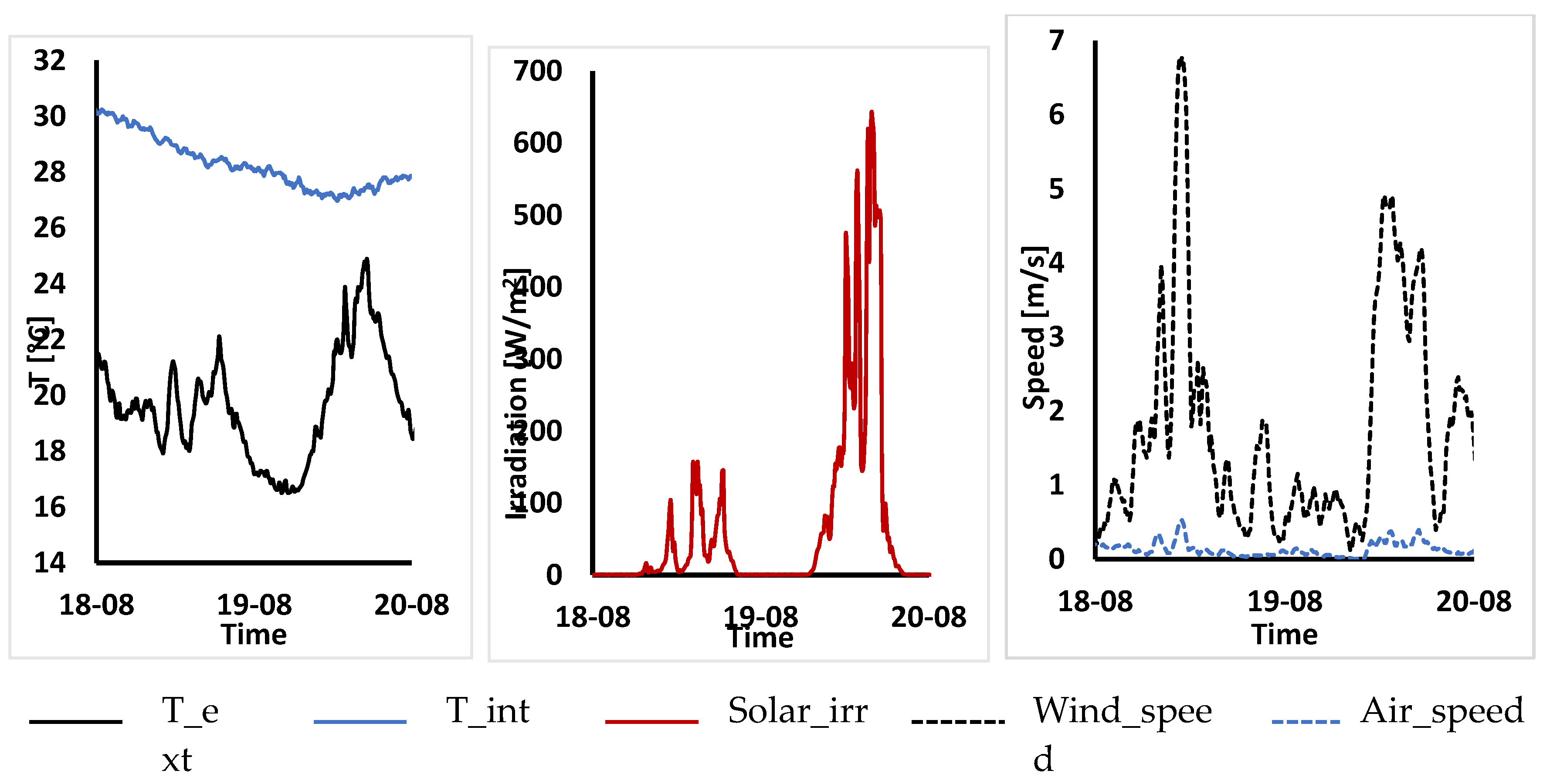
Figure A2.
Temporal evolution of the boundary conditions considered for summer cloudy days:
outdoor temperature (T_ext), indoor temperature (T_int), incident solar irradiation on the façade
(Solar_irr), wind speed (Wind_speed), air speed at the bottom opening of the ventilated cavity
(Air_speed).
Figure A2.
Temporal evolution of the boundary conditions considered for summer cloudy days:
outdoor temperature (T_ext), indoor temperature (T_int), incident solar irradiation on the façade
(Solar_irr), wind speed (Wind_speed), air speed at the bottom opening of the ventilated cavity
(Air_speed).
Appendix B – Algorithmic Details of the “Frozen Unfrozen Flow” Solver
In this appendix, more information about the algorithm of the “frozen-unfrozen flow” solver are given.
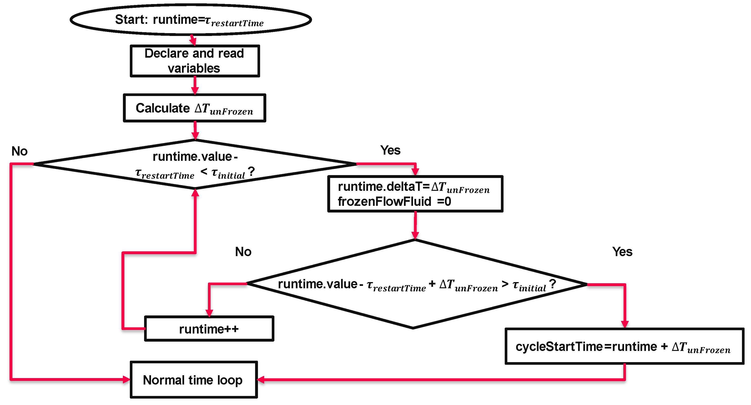
The Initial period is the timespan when the simulation starts from 0 (or from the latest saved time steps in case of simulation restart) and ends at the end of the specified initial time duration (i.e., ) defined in the “fluid.1/fvSolution” file. The algorithm in this period has the following features:
- declaration of the variables;
- calculation of the time-step based on courant and solid diffusion numbers;
- setting the Unfrozen mode for the fluid flow;
- setting the “cycleStartTime” at the end of this period.
Figure B1.
The algorithm for the initial period (τinitial) in the new solver.
The normal period when the flow solution mode is sequentially set to unfrozen and frozen. The sum of the frozen time () and unfrozen time () is called a cycle. The maximum time step (), and are user settings and are given in “fluid.1/fvSolution”.
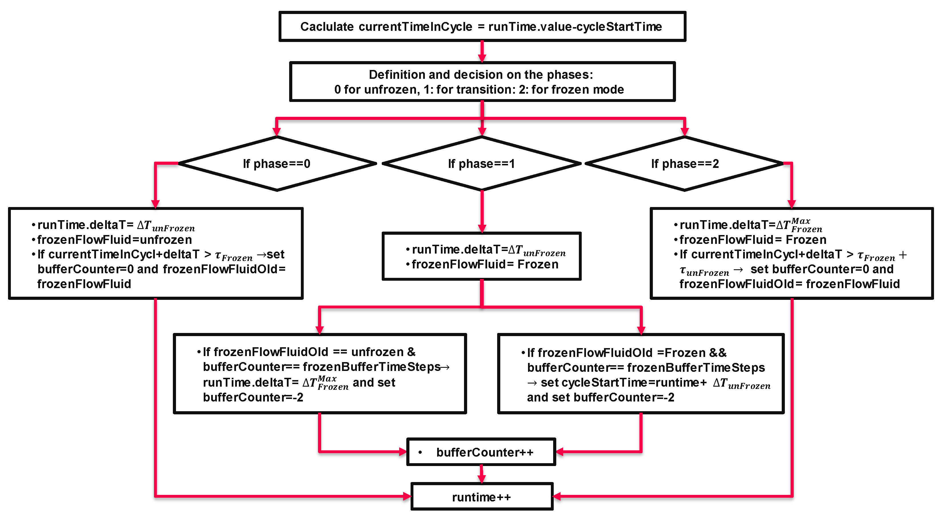
This period has the following features (see Error! Reference source not found.Error! Reference source not found.):
- it calculates the current time in a cycle (“currentTimeInCycle”), which is the difference between the current flow time and “cycleStartTime”;
-
it assigns the phases for frozen, unfrozen, or transition modes (see Error! Reference source not found.Error! Reference source not found.):
- ○
- if “bufferCounter” is equal to -1 and the runtime is in unfrozen mode, the phase is 0, otherwise, the phase is 2;
- ○
- if “bufferCounter” is not equal to -1, then set the phase to 1.
- if the phase is “0”, then set the time step to and the mode of the flow “unfrozen”. If the new flow time falls in a new phase, set “bufferCounter” to 0 and store the latest flow solution mode as “frozenFlowFluidOld”
-
if the phase is 1, then set the time step to , then decide based on the previous phase flow mode:
- ○
- if “frozenFlowFluidOld” is unfrozen and “bufferCounter” reaches the use input value (i.e. “bufferCounterSteps”), set the time step to and “bufferCounter” to -2;
- ○
- if “frozenFlowFluidOld” is frozen and “bufferCounter” reaches the use input value (i.e. “bufferCounterSteps”), then “bufferCounter”. to -2 and set “cycleStartTime” =current flow time + .
- if phase is 2 then, freeze the flow and set the time step to . Once the solution falls out of the cycle, set “bufferCounter” to 0 and store the latest flow solution mode as “frozenFlowFluidOld”
- repeat the above steps till the flow time reaches the end time of the simulation (defined in “controlDict”)
Figure B2.
The algorithm for the initial period (τinitial) in the new solver.
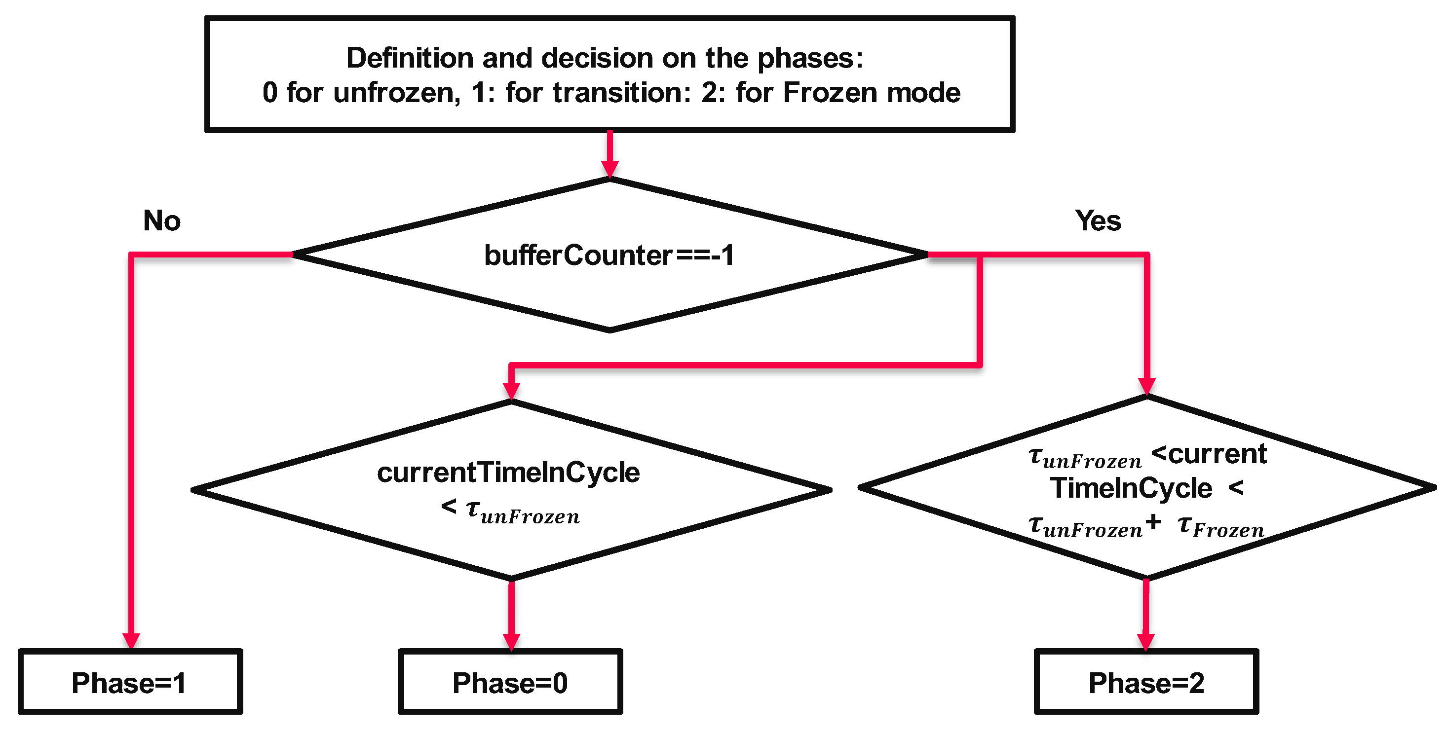
Figure B3.
The algorithm for the initial period (τinitial) in the new solver.
References
- Asdrubali, F.; Ferracuti, B.; Lombardi, L.; Guattari, C.; Evangelisti, L.; Grazieschi, G. A Review of Structural, Thermo-Physical, Acoustical, and Environmental Properties of Wooden Materials for Building Applications. . Build Environ 2017, 114, 307–332. [CrossRef]
- Janssen, H. Characterization of Hygrothermal Properties of Wood-Based Products – Impact of Moisture Content and Temperature. Constr Build Mater 2018, 185, 39–43. [CrossRef]
- Fortuna, S.; Mora, T.D.; Peron, F.; Romagnoni, P. Environmental Performances of a Timber-Concrete Prefabricated Composite Wall System. In Proceedings of the Energy Procedia; 2017; pp. 90–97.
- Pastori, S.; Mereu, R.; Mazzucchelli, E.S.; Passoni, S.; Dotelli, G. Energy Performance Evaluation of a Ventilated Façade System through Cfd Modeling and Comparison with International Standards. Energies (Basel) 2021, 14. [CrossRef]
- Destro, R.; Boscato, G.; Mazzali, U.; Russo, S.; Peron, F.; Romagnoni, P. Structural and Thermal Behaviour of a Timber-Concrete Prefabricated Composite Wall System. In Proceedings of the Energy Procedia; 2015; pp. 2730–2735.
- Patania, F.; Gagliano, A.; Nocera, F.; Ferlito, A.; Galesi, A. Thermofluid-Dynamic Analysis of Ventilated Facades. Energy Build 2010, 42, 1148–1155. [CrossRef]
- Fantucci, S.; Serra, V.; Carbonaro, C. An Experimental Sensitivity Analysis on the Summer Thermal Performance of an Opaque Ventilated Façade. Energy Build 2020, 225. [CrossRef]
- Marinosci, C.; Semprini, G.; Morini, G.L. Experimental Analysis of the Summer Thermal Performances of a Naturally Ventilated Rainscreen Façade Building. Energy Build 2014, 72, 280–287. [CrossRef]
- Melgaard, S.P.; Nikolaisson, I.T.; Zhang, C.; Johra, H.; Larsen, O.K. Double-Skin Façade Simulation with Computational Fluid Dynamics: A Review of Simulation Trends, Validation Methods and Research Gaps. Build Simul 2023, 16, 2307–2331. [CrossRef]
- Limane, A.; Fellouah, H.; Galanis, N. Thermo-Ventilation Study by OpenFOAM of the Airflow in a Cavity with Heated Floor. Build Simul 2015, 8, 271–283. [CrossRef]
- Horikiri, K.; Yao, Y.; Yao, J. Modelling Conjugate Flow and Heat Transfer in a Ventilated Room for Indoor Thermal Comfort Assessment. Build Environ 2014, 77, 135–147. [CrossRef]
- Brandl, D.; Mach, T.; Grobbauer, M.; Hochenauer, C. Analysis of Ventilation Effects and the Thermal Behaviour of Multifunctional Façade Elements with 3D CFD Models. Energy Build 2014, 85, 305–320. [CrossRef]
- Fantucci, S.; Marinosci, C.; Serra, V.; Carbonaro, C. Thermal Performance Assessment of an Opaque Ventilated Façade in the Summer Period: Calibration of a Simulation Model through in-Field Measurements. In Proceedings of the Energy Procedia; Elsevier Ltd, March 1 2017; Vol. 111, pp. 619–628.
- Chourdakis, G.; Schneider, D.; Uekermann, B. OpenFOAM-PreCICE: Coupling OpenFOAM with External Solvers for Multi-Physics Simulations. OpenFOAM® Journal 2023, 3, 1–25. [CrossRef]
- Laitinen, A.; Saari, K.; Kukko, K.; Peltonen, P.; Laurila, E.; Partanen, J.; Vuorinen, V. A Computational Fluid Dynamics Study by Conjugate Heat Transfer in OpenFOAM: A Liquid Cooling Concept for High Power Electronics. Int J Heat Fluid Flow 2020, 85. [CrossRef]
- Pastori, S. Timber-Concrete Composite Ventilated Envelope Systems. Experimental and Numerical Investigations for Thermal Performance Control and Optimization., Politecnico di Milano, 2024.
- EN ISO 10456:2007 Materials and Products - Hygrothermal Properties -Tabulated Design Values and Procedures for Determining Declared and Design Thermal Values.
- EN ISO 6946:2017 Components and Building Elements - Thermal Resistance and Thermal Transmittance - Calculation Methods.
- Kays, W.M.; Crawford, M.E. Convective Heat and Mass Transfer; McGraw-Hill, 1980;
- Tahmasebinia, F.; Lin, L.; Wu, S.; Kang, Y.; Sepasgozar, S. Exploring the Benefits and Limitations of Digital Twin Technology in Building Energy. Applied Sciences (Switzerland) 2023, 13. [CrossRef]
Figure 1.
Horizontal section of the TCC façade studied (units in cm). The layers are: 1) reinforced concrete slab; 2) ventilated air cavity; 3) OSB panel; 4) rockwool insulation (100 kg/m³); 5) timber-frame structure; 6) OSB panel. © Pastori S.
Figure 1.
Horizontal section of the TCC façade studied (units in cm). The layers are: 1) reinforced concrete slab; 2) ventilated air cavity; 3) OSB panel; 4) rockwool insulation (100 kg/m³); 5) timber-frame structure; 6) OSB panel. © Pastori S.
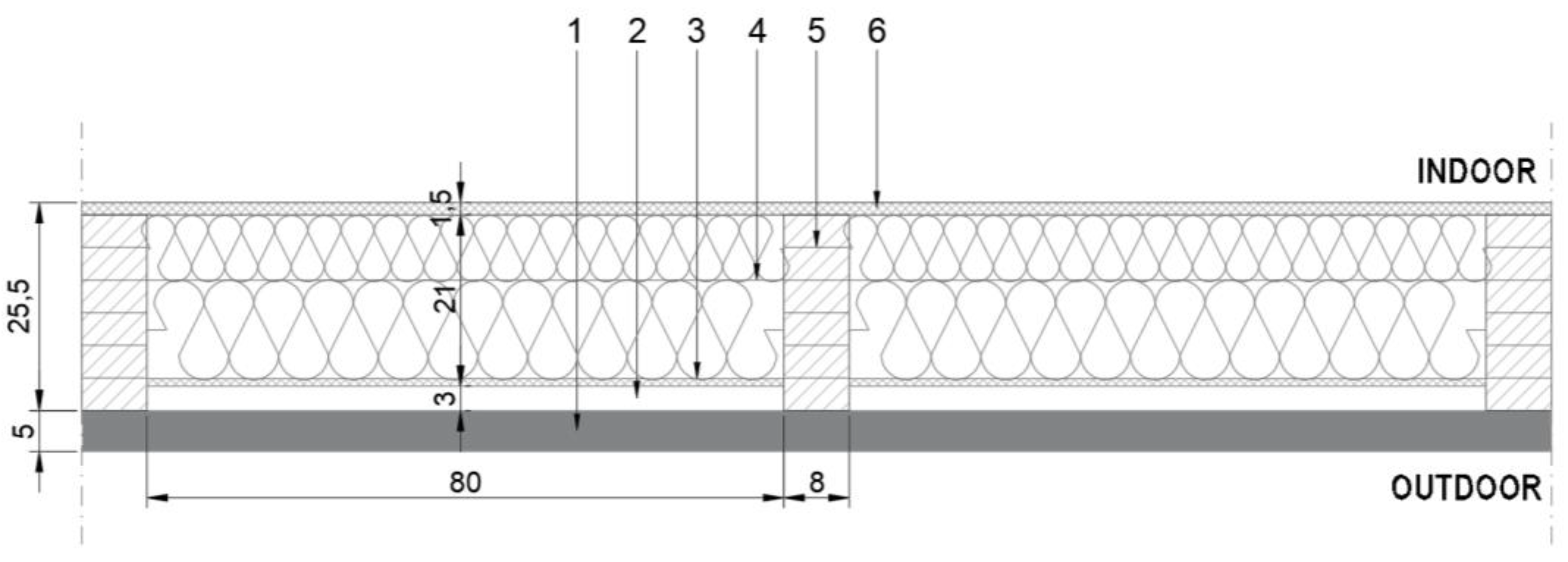
Figure 2.
Monitored building located in the north of Italy and identification of the TCC ventilated envelope area analysed. © Pastori S.
Figure 2.
Monitored building located in the north of Italy and identification of the TCC ventilated envelope area analysed. © Pastori S.
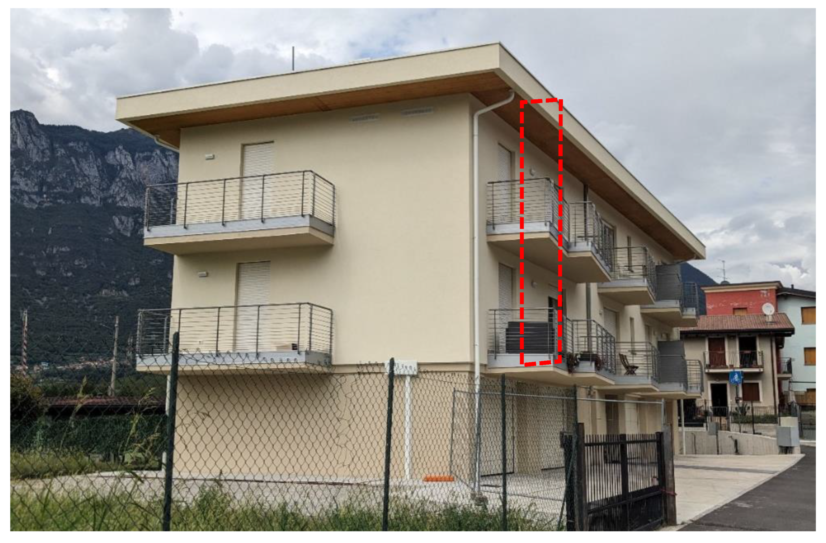
Figure 4.
Main boundary conditions used in the CFD model.
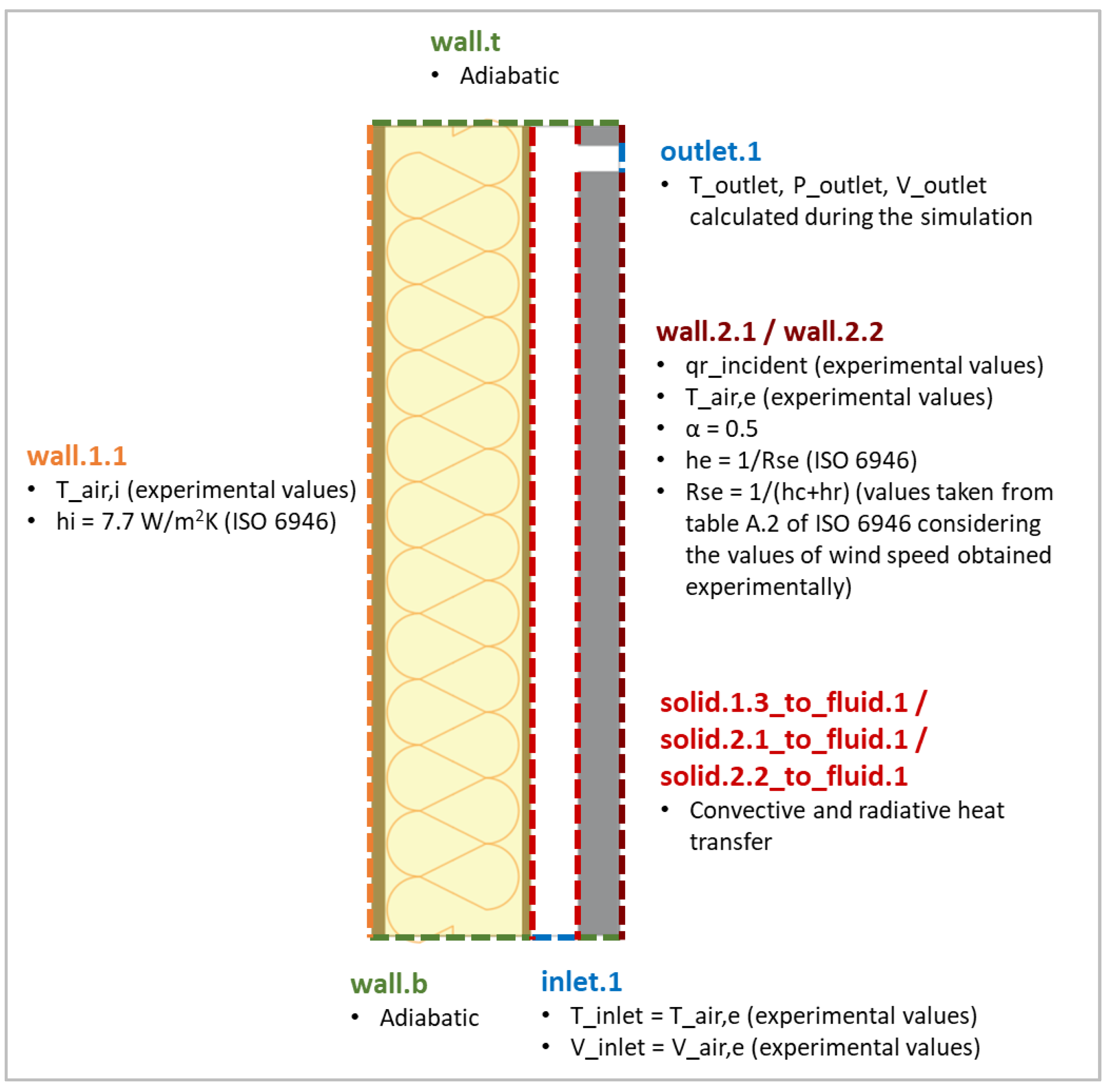
Figure 5.
Geometry and mesh of the 2D CFD model.
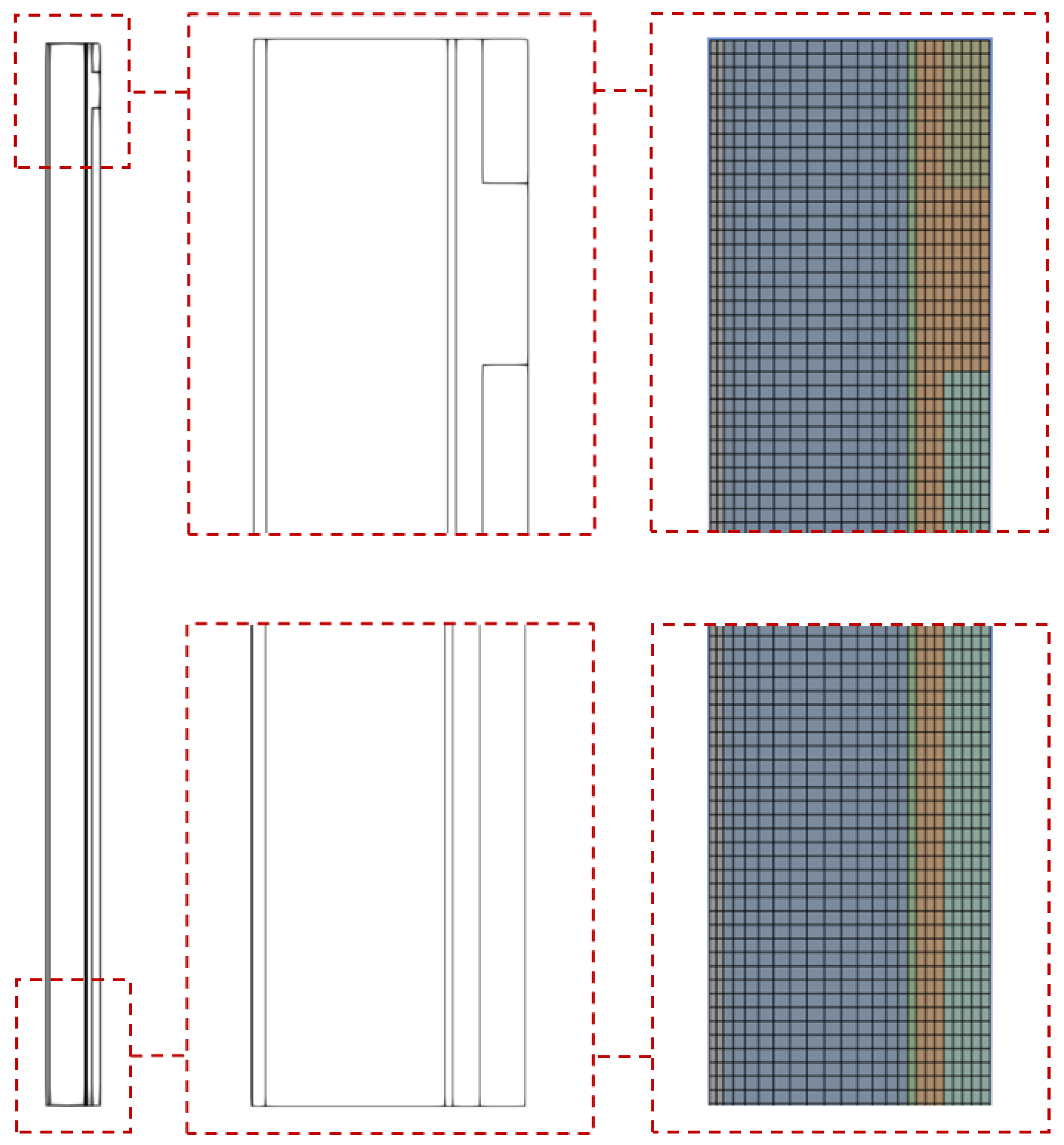
Table 1.
Physical properties of each region of the CFD model.
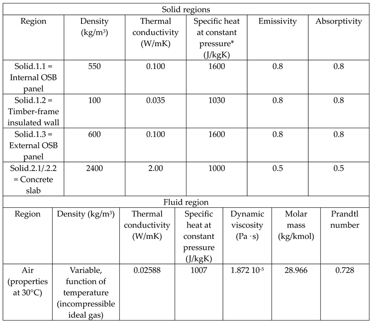
*values taken from EN ISO 10456 2007 [17.]
Table 2.
Results of the mesh refinement study.
| Mesh refinement study | |||||
| Simulation | Mesh | Solver | Time simulated | Time needed for running simulation | Temperatures that differ more than 0.2K from base case (t0001) |
| t0001 | m0012_baseMesh (7152 cells) |
chtMultiRegionFoam | 96h (345000 s) |
67.5h |
- |
| t0002 | m0013_baseMeshx1.5 (14850 cells) |
chtMultiRegionFoam | 48h (172800 s) |
100h (+196% than t0001) |
1.4% |
| t0003 | m0014_baseMeshx1.5x1.5 (33075 cells) |
chtMultiRegionFoam | 24h (86400 s) |
314h (+1761% than t0001) |
5.7% |
Table 3.
List of cases run for testing the new solver and finding the optimal settings considering the trade-off between speed and results accuracy.
Table 3.
List of cases run for testing the new solver and finding the optimal settings considering the trade-off between speed and results accuracy.
| Comparison between “frozen-unfrozen flow” solver and old solver | |||||||
| Case | tauFrozen/ tauUnfrozen |
Simulation speedup (24h real time compared to base case t0001) | Relative performance | Max temperature difference (K) from t0001 | % of values that differ more than 0.2K from t0001 | % of values that differ more than 0.5K from t0001 | % of values that differ more than 1K from t0001 |
| t0011 | 5s/5s = 1 | x 1.8 | 90% | -2.61 (in outlet.1) | 12.9% | 7.6% | 3.9% |
| t0012 | 10s/5s = 2 | x 2.7 | 90% | 3.61 (in outlet.1) |
15.5% | 8.0% | 4.1% |
| t0013 | 15s/5s = 3 | x 3.5 | 88% | -2.87 (in outlet.1) | 16.6% | 7.7% | 4.3% |
| t0014 | 50s/5s = 10 | x 9.4 | 85% | 3.20 (in outlet.1) |
12.4% | 2.8% | 1.0% |
| t0015 | 100s/5s = 20 | x 16.5 | 79% | 2.66 (in outlet.1) |
12.6% | 2.9% | 1.3% |
| t0016 | 500s/5s = 100 | x 45 | 45% | 3.43 (in outlet.1) |
20.8% | 9.9% | 4.5% |
Table 4.
Description of the cases run for the sensitivity analysis.
| Sensitivity analysis | |||
| Case | Goal | Physical parameters | Boundary conditions |
| t0101 |
Base case | Parameters reported in paragraph 3.2 | hToAmb = 1/Rse * hToAmbInt = 7.7 W/m2K qrIncident: summer sunny days, south Ta: summer sunny days TaRad: off (=Ta) Ti: summer sunny days U: summer sunny days |
| t0102 |
Change specific heat capacity for solid regions | 2xCp of solid regions | hToAmb = 1/Rse * hToAmbInt = 7.7 W/ m2K qrIncident: summer sunny days, south Ta: summer sunny days TaRad: off (=Ta) Ti: summer sunny days U: summer sunny days |
| t0103 |
Change solar irradiation values | 20% reduction of incident solar irradiation values | hToAmb = 1/Rse * hToAmbInt = 7.7 W/ m2K qrIncident: 0.8xqr,summer sunny days, south Ta: summer sunny days TaRad: off (=Ta) Ti: summer sunny days U: summer sunny days |
| t0104 |
Change of emissivity values for solid regions | 0.8xemissivity of solid regions | hToAmb = 1/Rse * hToAmbInt = 7.7 W/ m2K qrIncident: summer sunny days, south Ta: summer sunny days TaRad: off (=Ta) Ti: summer sunny days U: summer sunny days |
| t0105 |
Test how the model works with absence of solar irradiation | Incident solar irradiation switched off | hToAmb = 1/Rse * hToAmbInt = 7.7 W/ m2K qrIncident = 0 W/m2 Ta: summer sunny days TaRad: off (=Ta) Ti: summer sunny days U: summer sunny days |
| t0106 |
Change the type of heat exchange between the external surface of the wall and the outdoor environment, considering convective and radiative heat exchange separately. | Outdoor convective and radiative heat transfers are considered separately: qcv = hcv (Ta - TC_ext) qrd = ε σ Fw-sky (TC_ext4 - Tsky4) Tsky = 0.037536 Ta1.5 + 0.32 Ta |
hToAmb = 1/Rse * hToAmbInt = 7.7 W/ m2K qrIncident: summer sunny days, south Ta: summer sunny days TaRad: Tsky. csv Ti: summer sunny days U: summer sunny days |
| t0107 |
Change the type of heat exchange between the external surface of the wall and the outdoor environment, considering convective and radiative heat exchange separately. | Outdoor convective and radiative heat transfers are considered separately: qcv = hcv (Ta - TC_ext) qrd = ε σ Fw-sky (TC_ext4 - Tsky4) Tsky = 0.037536 Ta^1.5 + 0.32 Ta |
hcvToAmb =4+4v * hToAmbInt = 7.7 W/ m2K qrIncident: summer sunny days, south Ta: summer sunny days TaRad: Tsky. csv Ti: summer sunny days U: summer sunny days |
| t0108 |
Change the type of heat exchange between the external surface of the wall and the outdoor environment, considering convective and radiative heat exchange separately. | Option “hInclRad: false” | hToAmb = 1/Rse * hToAmbInt = 7.7 W/ m2K qrIncident: summer sunny days, south Ta: Ta,reduced.csv TaRad: off (=Ta) Ti: summer sunny days U: summer sunny days |
| t0109 |
Change specific heat capacity of solid regions | 1.5xCp for solid regions | hToAmb = 1/Rse * hToAmbInt = 7.7 W/ m2K qrIncident: summer sunny days, south Ta: summer sunny days TaRad: off (=Ta) Ti: summer sunny days U: summer sunny days |
| t0110 |
Change specific heat capacity of solid regions | 2xCp for solid region 2 1xCp for solid region 1 |
hToAmb = 1/Rse * hToAmbInt = 7.7 W/ m2K qrIncident: summer sunny days, south Ta: summer sunny days TaRad: off (=Ta) Ti: summer sunny days U: summer sunny days |
| t0111 |
Change thermal conductivity of solid regions | 2xCp for solid region 2 1xCp for solid region 1 0.5xlambda for solid regions |
hToAmb = 1/Rse * hToAmbInt = 7.7 W/ m2K qrIncident: summer sunny days, south Ta: summer sunny days TaRad: off (=Ta) Ti: summer sunny days U: summer sunny days |
| t0112 |
Change temperature values of outdoor air (Ta in °C) and specific heat capacity of solid regions | Ta,reduced = 0.6xTa 2xCp for solid region 2 1xCp for solid region 1 |
hToAmb = 1/Rse * hToAmbInt = 7.7 W/ m2K qrIncident: summer sunny days, south Ta: Ta,reduced TaRad: off (=Ta) Ti: summer sunny days, wall S3 U: summer sunny days, wall S3 |
| t0113 |
Change temperature values of outdoor air (Ta in °C) | TaReduced = 0.6xTa | hToAmb = 1/Rse * hToAmbInt = 7.7 W/ m2K qrIncident: summer sunny days, south Ta: Ta,reduced TaRad: off (=Ta) Ti: summer sunny days, wall S3 U: summer sunny days, wall S3 |
| t0114 |
Change temperature values of outdoor air (Ta in °C) | From 9am to 9pm: TaReduced,version2 = 0.6xTa From 9pm to 9am: TaReduced,version2 = 0.8xTa |
hToAmb = 1/Rse * hToAmbInt = 7.7 W/ m2K qrIncident: summer sunny days, south Ta: Ta,reduced,version2 TaRad: off (=Ta) Ti: summer sunny days, wall S3 U: summer sunny days, wall S3 |
| t0115 |
Change temperature values of outdoor air (Ta in °C), specific heat capacity and thermal conductivity of solid region 2 | TaReduced = 0.6xTa 1.5xCp for solid region 2 0.5xλ for solid region 2 |
hToAmb = 1/Rse * hToAmbInt = 7.7 W/ m2K qrIncident: summer sunny days, south Ta: Ta,reduced,version2 TaRad: off (=Ta) Ti: summer sunny days, wall S3 U: summer sunny days, wall S3 |
| t0116 |
Change temperature values of outdoor air (Ta in °C), specific heat capacity and thermal conductivity of solid region 2 | From 9am to 9pm: TaReduced,version2 = 0.6xTa From 9pm to 9am: TaReduced,version2 = 0.8xTa 1.5xCp for solid region 2 0.5xλ for solid region 2 |
hToAmb = 1/Rse * hToAmbInt = 7.7 W/ m2K qrIncident: summer sunny days, south Ta: Ta,reduced,version2 TaRad: off (=Ta) Ti: summer sunny days, wall S3 U: summer sunny days, wall S3 |
*Rse value was taken from EN ISO 6946 [18.]
Table 5.
List of the cases run in our sensitivity analysis, and error of the corresponding prediction by each case compared to the experimental results.
Table 5.
List of the cases run in our sensitivity analysis, and error of the corresponding prediction by each case compared to the experimental results.
| Results of the sensitivity analysis | |||||
| Case | Time needed for running simulation with old solver (h) | TO: error % between experiment and CFD | TC: error % between experiment and CFD | TC_ext: error % between experiment and CFD | Average error % |
| t0101 | 37 | 12 | 10 | 9 | 10.33 |
| t0102 | 32.5 | 8.75 | 4.96 | 10.97 | 8.23 |
| t0103 | 36 | 13 | 10 | 7 | 10.00 |
| t0104 | 36 | 12 | 10 | 8 | 10.00 |
| t0105 | 41 | 19 | 18 | 13 | 16.67 |
| t0106 | 39 | 18 | 18 | 16 | 17.33 |
| t0107 | 39 | 18 | 18 | 18 | 18.00 |
| t0108 | 33.5 | 14 | 14 | 13 | 13.67 |
| t0109 | 32 | 10 | 7 | 9 | 8.67 |
| t0110 | 31.5 | 8.85 | 5.19 | 11.00 | 8.35 |
| t0111 | 30.5 | 9.41 | 5.49 | 12.57 | 9.16 |
| t0112 | 28.5 | 10 | 6 | 9 | 8.33 |
| t0113 | 30.5 | 12 | 8 | 5 | 8.33 |
| t0114 | 30.75 | 11 | 8 | 6 | 8.33 |
| t0115 | 27.25 | 12 | 7 | 9 | 9.33 |
| t0116 | 29 | 11 | 6 | 9 | 8.67 |
Table 7.
Results of the validation study.
| Results of validation process | |||||
| Case | Error of TR prediction |
Error of TO prediction |
Error of TC prediction |
Error of TC_ext prediction |
Average error |
| t2000 (= t0104) | 0.73% | 13.99% | 10.06% | 8.14% | 8.23% |
| t4500 | 0.73% | 15.45% | 11.91% | 6.86% | 8.74% |
Table 8.
Relative importance of radiative heat transfer inside the cavity for two different time snapshots for the cases: t0104 and t4500.
Table 8.
Relative importance of radiative heat transfer inside the cavity for two different time snapshots for the cases: t0104 and t4500.
| Time (s) |
(°C) |
(°C) |
(°C) |
solid.1.3 to fluid.1 (W/m2) |
solid.2.1 to fluid.1 (W/m2) |
solid.1.3 (W/m2) |
solid.2.1 (W/m2) |
| case t0104 | |||||||
| 6:00 pm | 34.28 | 35.05 | 37.05 | 2.50 | 9.00 | -9.73 | |
| 8:00 am | 19.93 | 20.25 | 19.75 | 1.04 | -0.59 | -0.87 | 1.27 |
| case t4500 | |||||||
| 6:00 pm | 31.68 | 31.80 | 33.01 | 0.39 | 4.32 | 5.67 | - 6.09 |
| 8:00 am | 20.88 | 21.29 | 21.09 | 1.33 | 0.68 | 0.31 | 0.01 |
Disclaimer/Publisher’s Note: The statements, opinions and data contained in all publications are solely those of the individual author(s) and contributor(s) and not of MDPI and/or the editor(s). MDPI and/or the editor(s) disclaim responsibility for any injury to people or property resulting from any ideas, methods, instructions or products referred to in the content. |
© 2024 by the authors. Licensee MDPI, Basel, Switzerland. This article is an open access article distributed under the terms and conditions of the Creative Commons Attribution (CC BY) license (http://creativecommons.org/licenses/by/4.0/).
Copyright: This open access article is published under a Creative Commons CC BY 4.0 license, which permit the free download, distribution, and reuse, provided that the author and preprint are cited in any reuse.


