
Submitted:
23 April 2024
Posted:
25 April 2024
Read the latest preprint version here
Abstract
We can analyze the properties of the Collatz Conjecture by using Terras’ Theorem, and computational graphical calculations. To do this, we introduce the concept of “tree" which shows the relationship between the input and output positive integers of the Collatz process. This approach offers a novel way for determining the non-existence of loops and diverge trees through computer simulations.
Keywords:
collatz conjecture
; 3x+1 problem
; Terras Theorem
1. Introduction
Collatz Conjecture is if one considers the following process on an arbitrary positive integer: [3,4]
In the end, the final value will eventually reach the number 1, regardless of the initial positive integer chosen. For convenience, let us refer to applying Eq. (1) on any arbitrary positive integer as applying Collatz process.
2. Theory
There is a chain of a Collatz process if we start from an odd number,
So if we call as as as then,
If there is a chain of Collatz processes for a list of odd numbers from to , then by using ,
Let us define the function as exponents of 2 after factorization of n.
We can define , and . Then, by applying multiple Collatz processes to Eq.(9), we can obtain,
Lemma 1.
If we prove the Collatz Conjecture for all odd positive integers, it is equivalent to proving it for all positive integers.
Proof.
Let us assume that all odd positive integers converge to 1 after a finite number of steps in the Collatz process. Then, if we have an even number for some n, let . The number is odd. Therefore, also converges to 1 after k more steps than . □
According to Lemma II.1, to investigate the Collatz conjecture, we only need to examine the convergence properties of odd positive integers.
Definition 1.
The set of odd positive integers is defined as follows:
where n and k are integers greater than 1, and . The properties of is:
for all
According to Definition II.2, we can categorize the set of odd numbers as follows:
Now, let us make a function that maps each odd number to its order number.
Here n is the odd number, and represents its order number. For example, , indicating that 5 is the third odd number (1, 3, 5, 7...). We can define this function using the definition in Eq. (10).
Let us define this tree-like diagram as a tree with a converging value x.
Definition 2.
If we link two integers with an arrow from the input to the output value using Eq. (15) for all integers, it generates the diagram, which we call a “tree", denoted as . Here, represents the partial ordering based on Eq. (15),
Then tree has a several properties [5]:
- (1)
- is a well-founded partial ordering on T.
- (2)
- , the set is linearly ordered by .
- (3)
- , there exists such that and . Here, essentially means or .
Definition 3.
For arbitrary tree , if then A is called the converge value of the tree, and the tree is called “converge tree". However, if there is no such A then the tree is called “diverge tree".
3. Lemma and Theorem
3.1. Proof of Uniqueness of the Converge Tree
According to Definition II.2, when we apply the function to all positive odd integers, after k iterations, some values converge to 1. We can categorize these values into groups, denoted as . If we recursively apply multiple times and there exist some values of x that satisfy , then those values remain fixed throughout this recursive process.
Lemma 2.
For some positive integer x, to satisfy , the corresponding k values in Eq. (15) lie within a length-1 interval,
Proof.
Therefore, the condition to make X as a positive integer is:
If we want to make X as an integer, then the numerator of Eq. (19) should be divisible by the denominator of Eq. (19). Therefore, the numerator must be greater than the denominator.
And since we know that the integer multiplication of can not be an integer, k should exist within the range of two transcendental numbers Q and .
So, this proves the lemma. □
Next Eq. (19) can be expressed as,
If we want to make X as an integer, the odd number in the numerator should be divisible by the odd number in the denominator. Therefore the odd number of the numerator must be greater than that of the denominator.
Therefore, the available values of k should lie within the region:
To achieve this, first let us utilizing the lemmas.
Lemma 3.
Here,
Proof.
First, let us define:
By using Taylor Series expansion, [2]
Hence, we can rewrite the right-hand side of Eq. (29) as:
Therefore we want to show:
Here, ,
Then, for every u, there exists an x such that:
Then, for some , we have , where . Considering the periodicity properties of , there are two available values of x for each u. Let us define that when , then , and if , then .
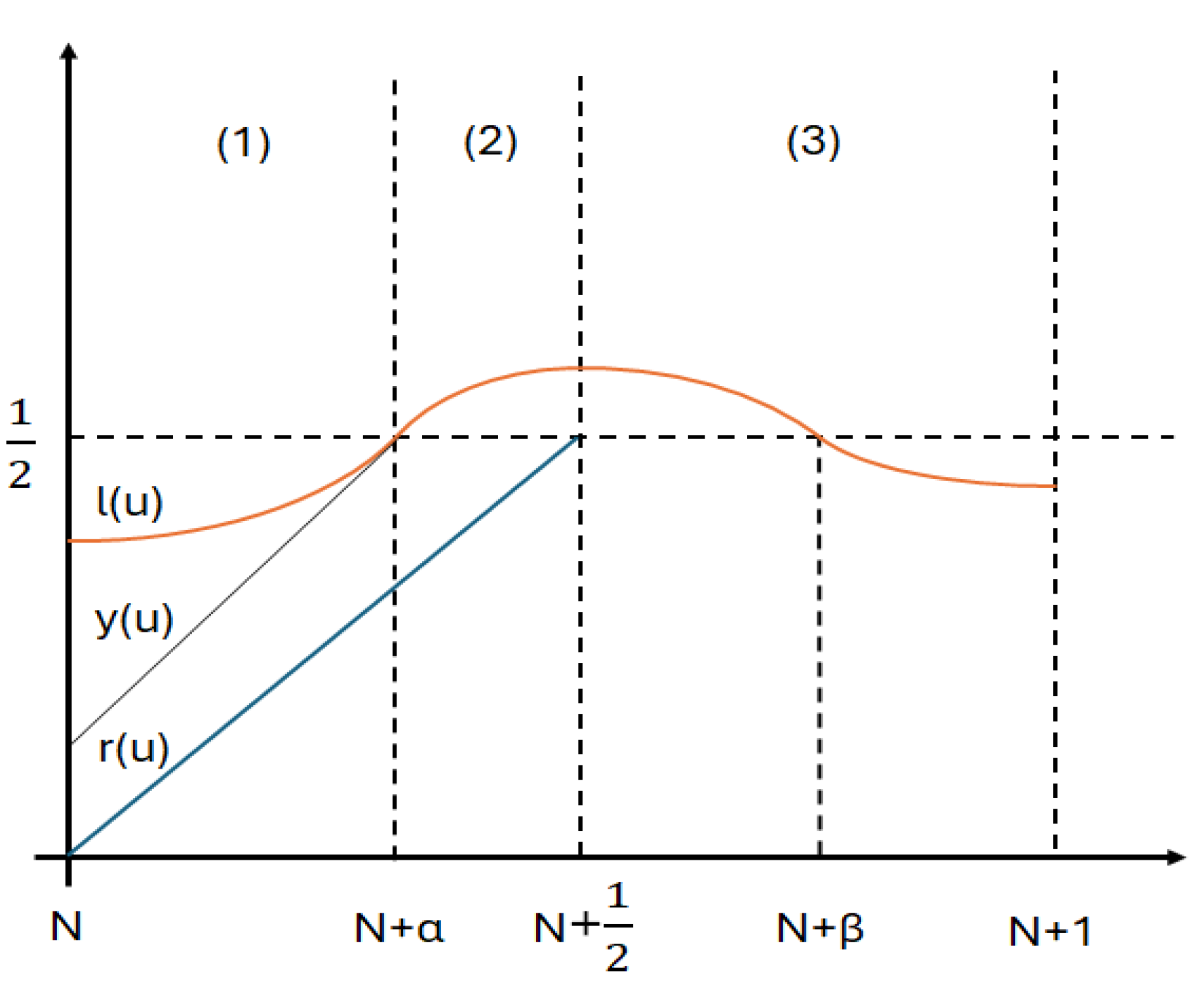
We can categorize the region of u into three regions.
- (1)
- (2)
- →
- (3)
- →
Figure 2.
Graphical representation of regions (1) to (3) and functions , , . Here, the x-axis represents u when .
Figure 2.
Graphical representation of regions (1) to (3) and functions , , . Here, the x-axis represents u when .
In regions (2) and (3), Eq. (36) is valid. In the case of region (1), let us calculate the tangential line of at .
Therefore, when , the line passes through the point,
because . Furthermore, Figure 3 shows that based on computer simulation, when , .
Therefore, in region (1), . Hence, Eq. (36) holds for all u, and Eq. (34) also holds. If we define:
then we can conclude that for any ,
We can use computer simulation to double-check that converges as we increase the values of N.
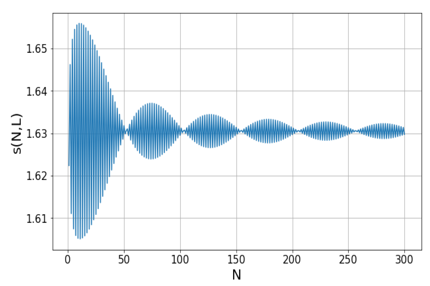
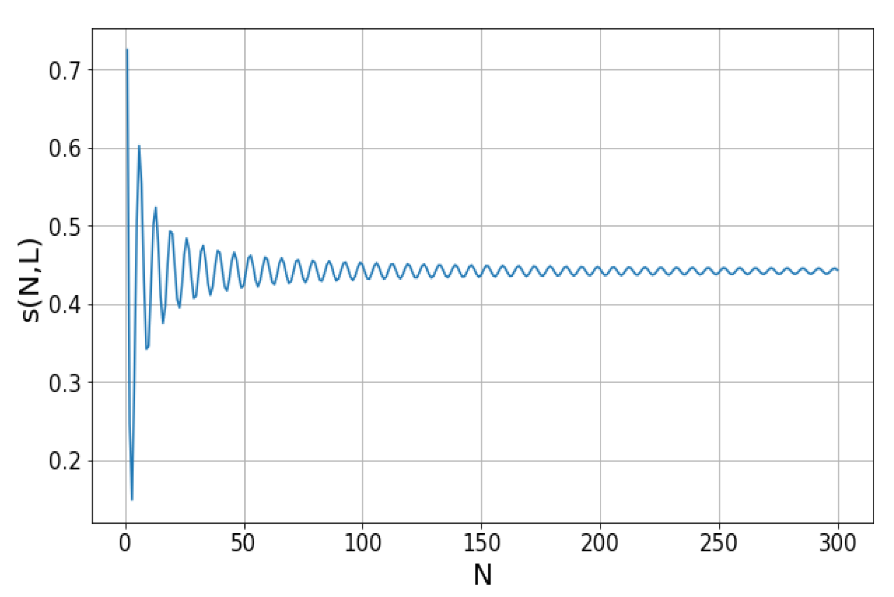
Figure 5.
The summation of the right-hand side of Eq. (39), which converges to positive real values, is calculated for N ranging from 1 to 300, and .
Figure 5.
The summation of the right-hand side of Eq. (39), which converges to positive real values, is calculated for N ranging from 1 to 300, and .
Figure 6.
The summation of the right-hand side of Eq. (39), which converges to positive real values, is calculated for N ranging from 1 to 300, and .
Figure 6.
The summation of the right-hand side of Eq. (39), which converges to positive real values, is calculated for N ranging from 1 to 300, and .
Based on computer simulation, we can double-check that converges as N increases, as shown in Figure 7. Therefore we can get,
Lemma 4.
Proof.
Let us set , then we can simplify Eq. (44) as
and if we use the floor function and fractional part function notation [6],
Here, we can utilize the Fourier series expansion of the fractional part function [7]:
Therefore, Eq. (46) is:
And we can get the range:
Let us find the region that satisfies:
The available range for L is:
And , which satisfying the condition. □
Theorem 1.
There is no positive integer point x that satisfies , except for .
Proof.
Theorem 2.
There is only one converge tree, and all elements in the converge tree converge to 1.
Proof.
Let us assume there is another converge tree with converging values . Then, since a is a converging value, we have . However, according to Lemma III.4 only 1 goes to itself, so is not an integer value other than a. This contradicts the assumption, thus confirming that there is only one converge tree in an integer system.
Therefore, there is only one converge tree, and if any integer is present in the converge tree, it will eventually converge to 1. □
3.2. Disproving the Existence of a Diverge Tree
Theorem 3.
There is no diverge tree.
Proof.
The part of the proof refers to [1] (1976) by R. Terras. Let us call as the set of all available converge trees. is the set of all available sets of diverge trees.
Let us assume . Then we can select the minimum element . For some k, if N is not a power of 2, then there always exists . Thus, we can express (). Since N is the minimum element of , we know that . According to Theorem III.5, converges to 1, and based on Definition 1.5 in [1], this implies that all x have a stop time except when . Here, stop time refers to the point at which, after a finite number of steps of the Collatz process, the value goes smaller than its initial value. For example, , the stop time is 3.
- (1)
- When , N also has the same stop time as b.
- (2)
- When , . If we apply the Collatz process, . If , . When , which also converges to 1.
- (3)
- When , applying the Collatz process results in convergence to 1, which is 1.
Therefore, in all cases, N also has a stop time. However, , so it should not have a stop time. This leads to a contradiction, so . □
4. Conclusion and Outlook
Theorem 4.
All positive integers converge to 1 after a finite number of steps of the Collatz process.
Proof.
According to Theorem III.5 and III.6, in a positive integer system, there is no diverge tree and there is only one converge tree, with the converging value 1. □
In this research, we prove that all positive integers converge to 1 after a finite number of steps of the Collatz process.
As an outlook, we can investigate the continuous generative function of Eq. (15) and the periodicity of the encoding vector of the numbers in Table 2. Additionally, there is another way of proving Lemma III.3 from Eq. (48), which is equivalent to show:
Then, with particular values of L, we can obtain:
Thus, to show the validity of Eq. (55) is the same as to show how quickly its right-hand side converges to 1 compared to . Moreover, besides this approach, various other methods such as cycle analysis [10] or bounding functions [11,12] are employed in the investigation of the Collatz conjecture. Exploring potential relations between these methods and the current result could be a relevant next step.
References
- Riho Terras, “A stopping time problem on the positive integers", ACTA ARITIMETICA (1976). http://matwbn.icm.edu.pl/ksiazki/aa/aa30/aa3034.pdf.
- Eric Roosendaal, “The Terras Theorem", http://www.ericr.nl/wondrous/terras.html.
- Jeffrey C. Lagarias, “The 3x + 1 problem and its generalizations". The American Mathematical Monthly. 92 (1): 3–23, (1985). [CrossRef]
- Jeffrey C. Lagarias, “The 3x+1 Problem: An Overview", 2021, https://arxiv.org/abs/2111.02635.
- Spencer Unger, “Trees in set Theory", https://www.math.toronto.edu/sunger/cmu/TreesTalk.pdf.
- R. L. Graham, D. E. Knuth, O. Patashnik, “Concrete Mathematics", Addison-Wesley (1994), p. 70.
- E. C. Titchmarsh, D. R. Heath-Brown, “The Theory of the Riemann Zeta-function" (2nd ed.), Oxford U. P. (1986), p. 15, Eq. 2.1.7.
- OEIS, “Decimal expansion of log_2(3)", https://oeis.org/A020857.
- Simon Plouffe, “log(3)/log(2) to 10000 digits", https://www.plouffe.fr/simon/constants/log3log2.txt.
- Shalom Eliahou, “Le problème 3n+1: y a-t-il des cycles non triviaux? (III)", Images des Maths, CNRS (2011).
- Terence Tao, “Almost all orbits of the Collatz map attain almost bounded values.", Forum of Mathematics (2022). [CrossRef]
- Ilia Krasikov, Jeffrey C. Lagarias “Bounds for the 3x+1 problem using difference inequalities". Acta Arith., 109, 237–258. (2003). [CrossRef]
Figure 1.
A diagram expression of Table 2 with directed arrows.
Figure 1.
A diagram expression of Table 2 with directed arrows.
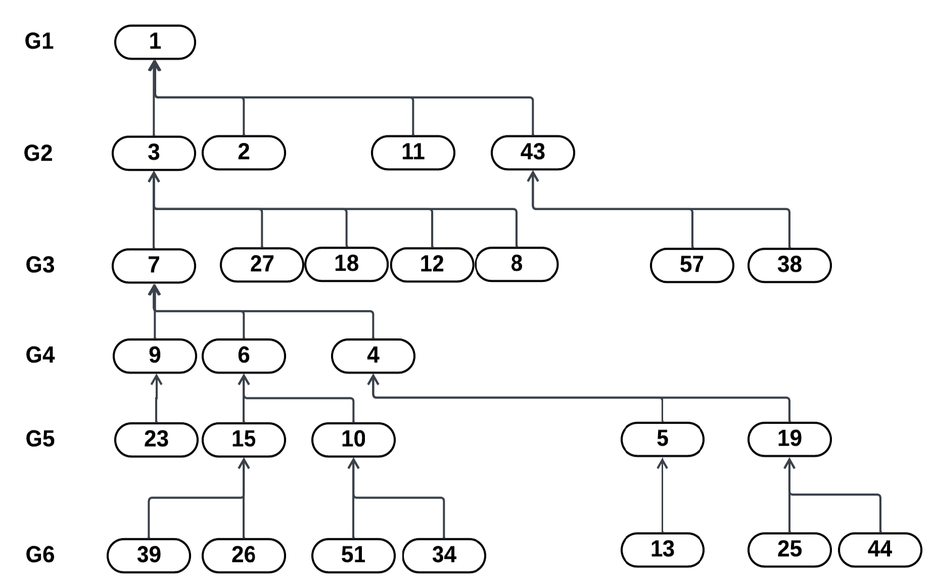
Figure 3.
The results of in the region where . Except for the case , all other graphs yield positive results across all regions.
Figure 3.
The results of in the region where . Except for the case , all other graphs yield positive results across all regions.
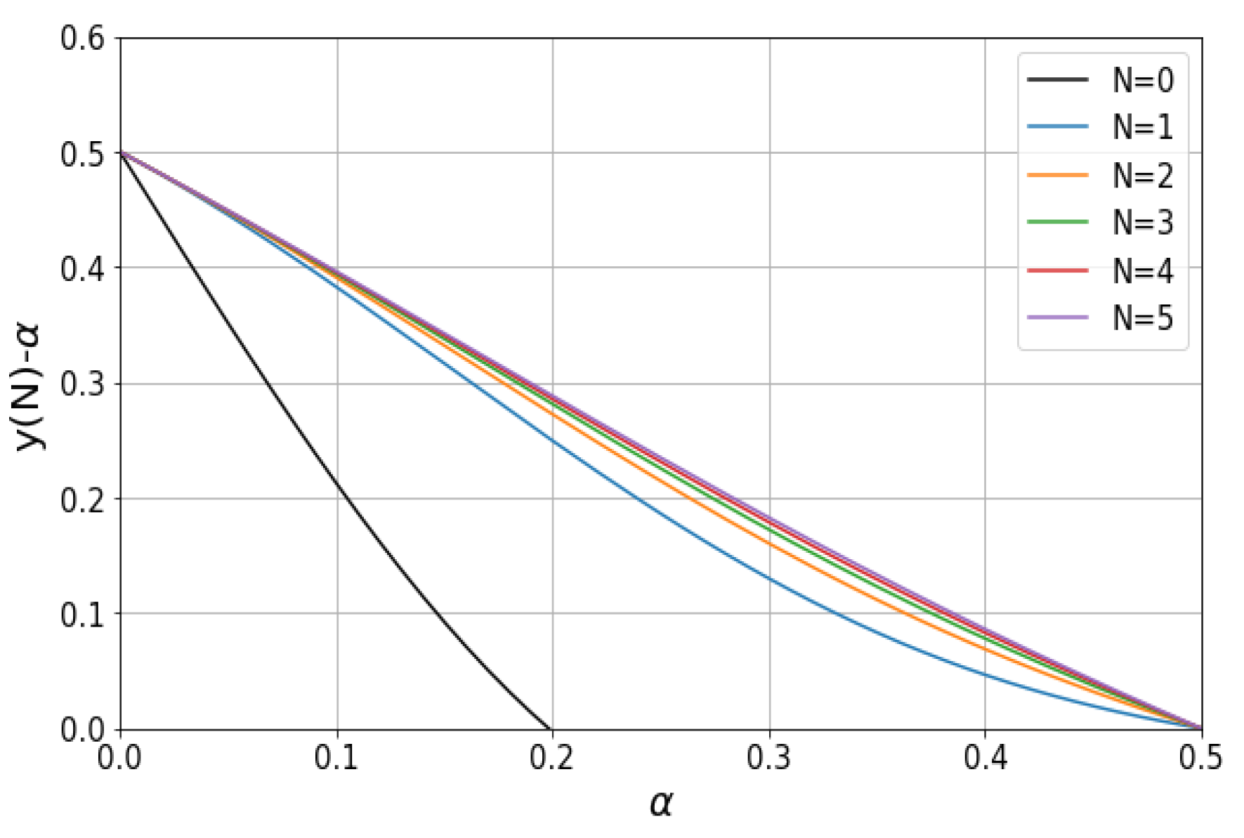
Figure 4.
The summation of the right-hand side of Eq. (39), which converges to positive real values, is calculated for N ranging from 1 to 300, and .
Figure 4.
The summation of the right-hand side of Eq. (39), which converges to positive real values, is calculated for N ranging from 1 to 300, and .
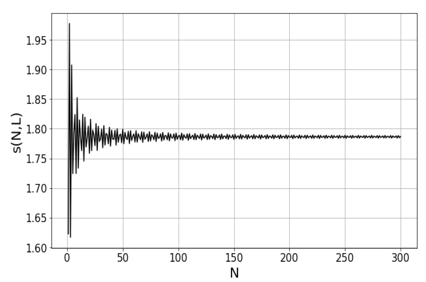
Figure 7.
The summation of the right-hand side of Eq. (39), which converges to positive real values, is calculated for L ranging from 1 to 1000, and .
Figure 7.
The summation of the right-hand side of Eq. (39), which converges to positive real values, is calculated for L ranging from 1 to 1000, and .
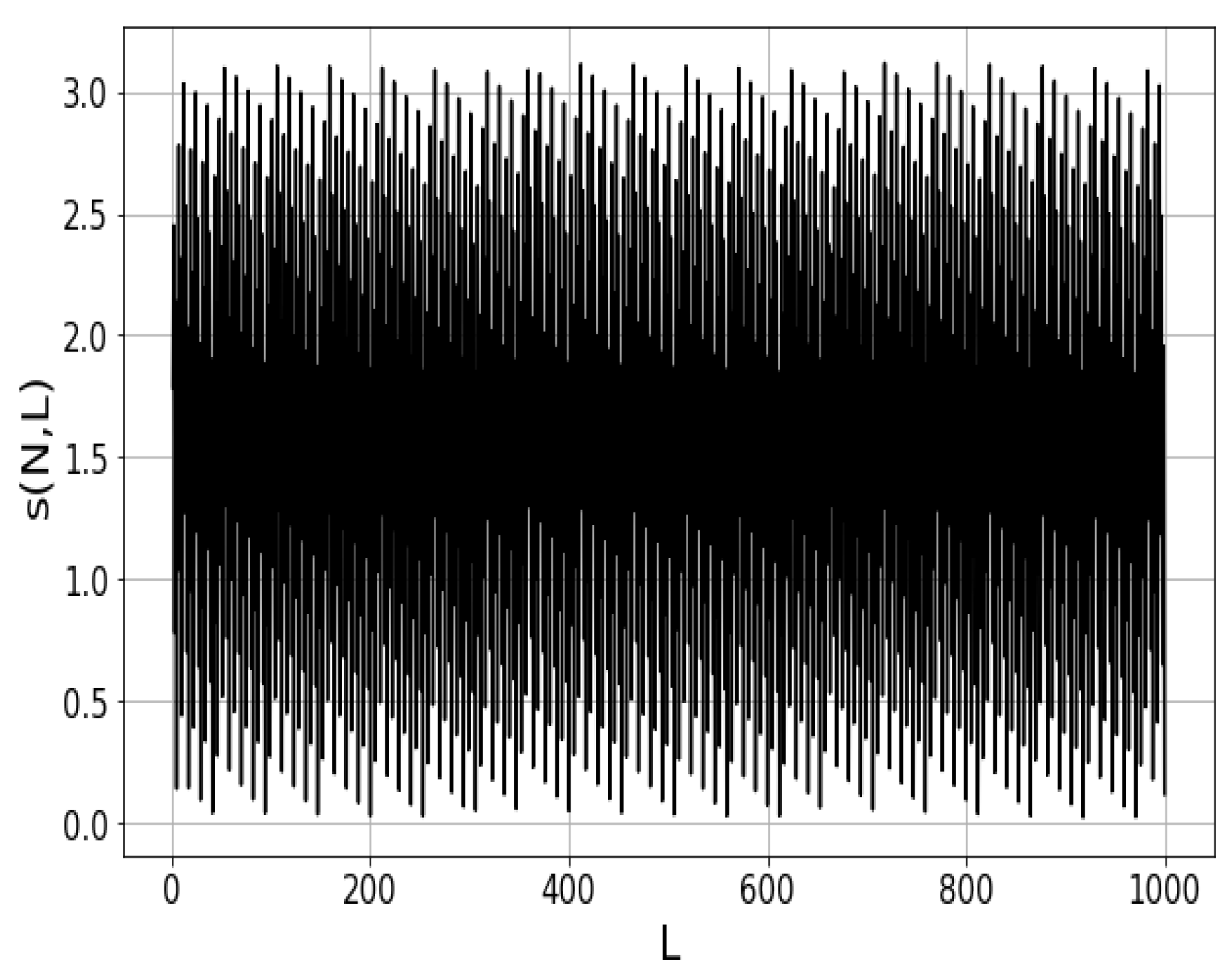

Table 1.
The categorization of odd numbers, (eg. to ).
| 1 | |
|---|---|
| 3, 5, 21, 85, 151, 227, 341... | |
| 13, 15, 23, 35, 53, 75, 113... | |
| 7, 11, 17, 61, 69, 93, 141... | |
| 9, 19, 29, 37, 45, 81, 117... | |
| 25, 49, 51, 67, 77, 87, 101... | |
| 33, 39, 43, 59, 65, 79, 89... | |
| 57, 105, 115, 157, 173, 177, 211... | |
| 127, 135, 139, 153, 159, 187, 191... | |
| 123, 169, 185, 247, 249, 283, 339... | |
| 111, 167, 219, 223, 225, 251, 295, 329... | |
| 297, 351, 393, 445, 527, 585, 595... | |
| 175, 263, 395, 519, 593, 615, 699... | |
| 103, 155, 207, 233, 311, 467, 701... | |
| 91, 137, 183, 275, 413, 549, 621... | |
| 63, 95, 121, 143, 215, 243, 323... | |
| 31, 47, 71, 107, 161, 253, 381... | |
| 27, 41, 55, 83, 125, 165, 189... | |
| 73, 109, 147, 195, 199, 221, 291... | |
| 97, 145, 259, 265, 387, 389, 471... | |
| 129, 193, 235, 240, 343, 345, 353... | |
| 171, 240, 257, 313, 415, 427, 457... | |
| 379, 417, 427, 543, 553, 569, 609... |
| 1 | |
|---|---|
| 2, 3, 11, 43, 76, 114, 171... | |
| 7, 8, 12, 18, 27, 38, 57... | |
| 4, 6, 9, 31, 35, 47, 72... | |
| 5, 10, 15, 19, 23, 41, 59... | |
| 13, 25, 26, 34, 39, 44, 51... | |
| 17, 20, 22, 30, 33, 40, 45... | |
| 29, 53, 58, 79, 87, 89, 106... | |
| 64, 68, 70, 77, 80, 94, 96... | |
| 62, 85, 93, 124, 125, 142, 170... |
Disclaimer/Publisher’s Note: The statements, opinions and data contained in all publications are solely those of the individual author(s) and contributor(s) and not of MDPI and/or the editor(s). MDPI and/or the editor(s) disclaim responsibility for any injury to people or property resulting from any ideas, methods, instructions or products referred to in the content. |
© 2024 by the authors. Licensee MDPI, Basel, Switzerland. This article is an open access article distributed under the terms and conditions of the Creative Commons Attribution (CC BY) license (http://creativecommons.org/licenses/by/4.0/).
Copyright: This open access article is published under a Creative Commons CC BY 4.0 license, which permit the free download, distribution, and reuse, provided that the author and preprint are cited in any reuse.


