Submitted:
20 April 2024
Posted:
22 April 2024
You are already at the latest version
Abstract
The superconductivity of CaC6 as a function of pressure and of abundant Ca isotopes is revisited using DFT calculations on a 2c – double hexagonal superlattice. The introduction of superlattices is motivated by previous synchrotron absorption and Raman spectroscopy results on other superconductors that show evidence of superlattice vibrations at low (THz) frequencies. A 2c superlattice for CaC6 is illustrative of atomic orbital symmetry and periodicity, including bonding and antibonding s-orbital character implied by cosine modulated electronic bands. Inspection of the cosine band reveals that the cosine function has a small (meV) energy difference between bonding and antibonding regions relative to a midpoint non-bonding energy. Fermi surface nesting is apparent in an appropriately folded Fermi surface using a superlattice construct. Nesting relationships identify phonon vectors for conservation of energy and for phase coherency between coupled electrons at opposite sides of the Fermi surface. Detailed analysis of this Fermi surface nesting provides accurate estimates of the superconducting gaps for CaC6 with change in applied pressure. Recognition of superlattices within a rhombohedral or hexagonal representation provides consistent mechanistic insight on superconductivity and electron−phonon coupling in CaC6.
Keywords:
Superconductivity
; CaC6
; Fermi surface
; Fermi level
; superlattice
; tight binding
; cosine
; band structure.
1. Introduction
Superlattices, quantum wells and other related nanoscale heterostructures have played, and continue to play, important roles in technological applications, such as resonant tunnelling devices and lasers [1,2,3]. Many familiar superlattices are layered, nanoscale periodic structures of two materials, resulting in compositional and/or lattice spacing modulations perpendicular to the layers. Modulations and new periodicities introduced to artificial superlattices can also be engineered to advantageously modify electronic properties and material behaviour [1,2,3]. More recent styles of superlattices, such as Moire-like [4,5,6] and ordered arrays of nanocrystals [7,8,9], have also been experimentally fabricated and/or used conceptually to explain observed electronic phenomena.
Superlattice concepts are used to explain phenomena closely related to superconducting materials, particularly the tuning of properties in the proximity of electronic topological transitions (ETTs) and Feshbach resonances as a function of pressure and strain, as well as the appearance of van-Hove singularities [10,11]. In addition, superlattices have been used to model striped structures, experimentally observed in superconductors at both nano [12] and atomic [13] scales. The effects of modulated strain in superconducting materials, both from the intrinsic crystal structure of the complex metal oxide [3] or artificially created to mimic those strain modulations [14], are also linked to superlattice observations and models.
Experimental observations of superlattice vibration modes in synchrotron THz absorption spectroscopy [15] and Raman spectroscopy [16] on MgB2 compounds, characterised by vibration modes of low frequency, have provided complementary numerical and mechanistic insights on the superconductivity of MgB2. These low frequency modes are substantially below the lowest absorption frequency predicted for the conventional P6/mmm symmetry ascribed to MgB2 based on atomic positions [15,17]. Recognition of a superlattice in MgB2 enabled identification of bonding and antibonding regions, and the role of Fermi surface (FS) nesting and phase relationships not otherwise apparent [15,18].
For layer structured superconductors, cosine shaped electronic bands are important indicators of conduction mechanisms. These cosine bands resemble tight-binding descriptors for the electronic bands of semiconductors [18]. However, for many superconductors the bonding (lower energy) and antibonding (higher energy) regions of the cosine amplitudes are marginally asymmetric.
We evaluate the asymmetry of cosine electronic bands for CaC6 using DFT calculations with high grid resolution and demonstrate a direct correlation to the superconducting gap at different pressures. The CaC6 superconductor [19,20] is an hexagonal layered compound with lower axial symmetry than MgB2. This compound can be described in either hexagonal or rhombohedral lattices [19]. We utilise both types of lattices in this paper to demonstrate the equivalence of results and to highlight specific features. In addition, we consider the importance of phonon dispersions and the critical role played by acoustic phonons in superconductivity.
2. Materials and Methods
We conducted a comprehensive DFT analysis on the Electronic Band Structures (EBSs) and FSs for CaC6 within a pressure range from 0 GPa up to 16 GPa using Quantum ESPRESSO [21] and Materials Studio CASTEP [22] for comparison. This analysis is detailed in a separate article. Key parameters such as plane wave cut-off energies, pseudopotentials, and k-point grids are critical enablers of meV resolution for EBS and phonon dispersion (PD) calculations as noted in earlier publications [17,23].
We employed cut-off energies of 120 Ry (= 1632.68 eV), a k-point grid of 24×24×24 sampling density, ultrasoft pseudopotentials [24] and with a generalised gradient approximation (GGA) [25,26] for the exchange-correlation functional. We also explored norm-conserving pseudopotentials within the LDA and GGA approximations for additional comparisons. DFT calculations considered both a primitive rhombohedral unit cell and the hexagonal counterpart. The specific lattice constants are taken from X-ray diffraction results of bulk CaC6 [19]. We have also explored several superlattice variants, acknowledging their significance in accurately portraying symmetry and phases of the orbitals [18]. Further evaluation of essential parameters that enable systematic detailed interpretation of DFT calculations are provided in our earlier work [23,27]. For consistency, we show calculation outputs using the LDA functional although equivalent calculations using the GGA functional show similar trends.
Constructing a supercell is a routine procedure for DFT calculations of electronic properties, although the context can differ substantially. For example, a supercell can be a “multiple of the smallest unit cell” or “a unit cell of a superlattice” structure. We initially build a supercell as a multiple of the smallest unit cell, and then we impose reduced symmetry that contains symmetry elements of the parent space group as shown in earlier work [16,28].
In a dynamic environment, we may also consider other forms of a superlattice. For example, an elastic acoustic wave imposed on an initially symmetric, homogeneous structure [7,29,30]. In this case, at a particular instant of time, there will be a modulated expansion and contraction of sub-units (e.g. the original smallest units) of a superlattice. According to elastic theory, the structure will show a modulation of the lattice constants with a wavelength given by the acoustic wavelength. A positional modulation of atoms will create a superlattice.
The smallest superlattice that can be created by elastic waves is a double unit supercell, where one cell is contracted, and the other adjacent cell is expanded. In general, a cosine shaped band in an EBS, particularly in superconductors, can be associated with nearly free electrons [31]. Such a band corresponds to a cosine wavefunction; that is, the real part of a plane wave or complex exponential. Thus, the electron density in that cosine band is modulated as the square of the cosine function and is periodically modulated as a superlattice structure.
3. Results and Discussion
In our earlier work on MgB2, we show that atomic orbital symmetry provides added detailed mechanistic understanding of superconductivity [18] compared with atomic position symmetry of space group P6/mmm. We utilise a similar strategy for DFT calculations on CaC6 by first, identifying key bands – particularly along an equivalent real space layer direction – that demonstrate a cosine format across or near the Fermi level. We develop an argument for construction of a double supercell, starting with a band that approximates a cosine function. Using a double cell for DFT calculations, several features related to superconductivity of CaC6 are derived in a fashion consistent with that previously described for MgB2 [15,18].
3.1. Cosine Functions and Linear Chains of Atoms
There is strong agreement that cosine shaped bands in the EBS of CaC6 as shown in Supplemental Figure S1 show nearly free Ca 4s orbital character [31]. The cosine function for the electronic band has argument ckz, implying that planes separated by lattice parameter c are out of phase [32]. This phase relationship in the c-direction is identical to that encountered in discussions on chain(s) of atoms with s-orbitals [33,34], as exemplified by a chain of H-atoms or H ‘n-merization’ [35]. A schematic of this important phase relationship and change from predominantly bonding to predominantly antibonding states is shown in Figure 1.
For a group symmetry to appropriately represent the periodicity implied by an antibonding orbital arrangement, a reduced symmetry with a double supercell in the c-direction must be used [15,18]. In this case, reduced symmetry is a better representation of a compound for which the orbital character of electrons and likely effects on atomic positions are considered. This representation is analogous to that shown for MgB2 [15,18], noting that for the c and ab- directions at Γ, the bands show opposite bonding/antibonding character (see e.g., Figure 1 of reference [18]). In contrast, for CaC6, in both the c and ab- directions at Γ, the bands show the same bonding character. This band characteristic is reasonable for s-orbitals with local spherical symmetry; thus, the same orbital character is maintained in the entire set of spherical directions.
3.2. Electronic Band Structures for Superlattices
We have calculated the EBS for three types of CaC6 unit cells of Space Group 166 (R-3m) at a pressure 0 GPa (i) a rhombohedral lattice, (ii) an equivalent hexagonal lattice of the same Space Group 166 and (iii) an equivalent hexagonal lattice with a double c-axis, 2c. In reciprocal space, a key visualisation format for EBS and Brillouin zones, doubling a real space dimension (e.g. a unit cell dimension, c, increased to 2c) can be effected by folding along the appropriate reciprocal direction [36]. For the hexagonal lattice of Space Group R-3m, the Γ–Z direction is along c*. Hence, the focus of this work is along the Γ–Z directions in reciprocal space. Calculated EBSs for conventional reciprocal directions for each CaC6 format are provided in Figures S1-S3 in Supplemental. The key c* directions that contain cosine-shaped band(s) are identified in Figures S1-S3.
3.3. Antibonding-Bonding Asymmetry
Careful inspection of the shape for the interlayer cosine band of CaC6 using rhombohedral structure (Space Group 166 or R-3m) indicates that the cosine function is not perfectly symmetric (see Figure 2a and Figure S1). We delineate this asymmetry as previously discussed in our evaluation of cosine sigma bands for MgB2 [18]. Asymmetry of a cosine band suggests that adjustments to tight binding equations are appropriate in order to describe the electronic band along the c*direction [18] as shown below.
An asymmetry, or difference in energy, ΔE, is schematically shown for CaC6 at 0 GPa calculated with a rhombohedral lattice in Figure 2a. Bonding and anti-bonding nodes, denoted “B” and “A”, respectively, of the cosine band along Γ–Z are shown in Figure 2a. The energy, Ec*/2, at the intersection of the cosine band with the reciprocal mid-point, ΓZ/2, is -193.5 meV. The average energy, Eav, between bonding (B) and antibonding (A) nodes at Γ and at Z, respectively, is 43.5 meV higher than Ec*/2 (i.e. at -150.0 meV) and denoted by a red horizontal line. This difference in energy, ΔE, represents the asymmetry of the cosine band for this rhombohedral lattice. A perfectly symmetric cosine band will show zero difference in energy between Ec*/2 and Eav (i.e. for equivalent bonding and antibonding regions. In the following sections, we describe how a superconducting gap can be determined from this antibonding–bonding energy asymmetry.
Figure 2b shows the band structure along the c* direction for an hexagonal lattice equivalent to the rhombohedral configuration shown in Figure 2a. In this case, there is a folding of the c* direction because the a and b directions are multiples of C-C bonds in CaC6. This folding results in two distinct bonding and antibonding nodes in the band structure as identified in Figure 2b. The energy at the intersection of the Aʹ–Bʹ band at ΓA/2 is Ec*/2 and denoted by a blue horizontal line in Figure 2b. For the hexagonal case, we determine Eav for both A–B and Aʹ–Bʹ as shown by the red horizontal lines in Figure 2b. The asymmetries, or ΔʹE and ΔE, are 10.3 meV and 43.5 meV (ΔE=10.3+33.2 meV), respectively, relative to the energy at Ec*/2.
Figure 3 shows the band structure along the c* direction for CaC6 at 0 GPa and at 7.5 GPa with an hexagonal 2c superlattice. For 2c superlattice symmetry, the Brillouin zone boundary line of the unfolded reciprocal space folds onto the Γ-direction. In an ideal structure, bonding and antibonding bands will adopt a symmetric appearance relative to the mid-point energy (i.e., with the symmetry axis at constant energy, Ec*/2) as shown by the blue horizontal line in Figure 3a (inset). In Figure 3a, Ec*/2 is now at the intersection on Z where the two branches of the cosine curve from Aʹ and Bʹ meet (i.e. blue line clearly shown in the inset). The energy for Ec*/2 is at a nominally lower energy (~5 meV) compared with Ec*/2 for the hexagonal cell shown in Figure 2b. Again, measuring the values for Eav and Eʹav as shown in Figure 3a, the difference in energy for ΔʹE and ΔE, are 10.3 meV and 43.5 meV (=10.3+33.2 meV), respectively (inset, Figure 3a; red lines relative to the blue line).
A similar configuration for the folded cosine band of a 2c superlattice at 7.5 GPa is shown in Figure 3b. In this case, the folded band along c* is at higher energy compared with calculations at 0 GPa, consistent with experimental data showing a higher Tc at 7.5 GPa [38]. Similar trends are observed for DFT calculations of hexagonal 2c superlattices at other pressures (Supplemental Figure S4).
3.4. Revised Tight-Binding Equations
To accommodate the condition for CaC6, we propose the following adjustments to tight binding equations of the form shown in equations (1) and (2):
The highest asymmetry offset at the Γ-direction is given by the equation:
where ETB Gap@Γ is a tight binding gap. Asymmetry values or tight binding gaps vary with respect to the choice of unit cell symmetry or type of supercell. However, the values are interrelated by the symmetry relationships between the hexagonal and rhombohedral lattice systems.
The dependence of Eav as function of kz, Eav(kz) is shown in Figure 4. Eav(kz) has a cosine dependence itself, with half the reciprocal space period of that for the cosine shaped band (= ½*2π/c = 2π/2c), and for a bonding-antibonding format of the Eav(kz) cosine we halve this reciprocal distance (=2π/4c). That is, in real space, the periodicity is double that of the bonding-antibonding folded periodicity (= 2*2c = 4c). A 4c superlattice periodicity has previously been identified for MgB2 [15,18]. This result suggests that the origin of this super-periodicity also relates to electronic behaviour, as represented by the electronic band structure.
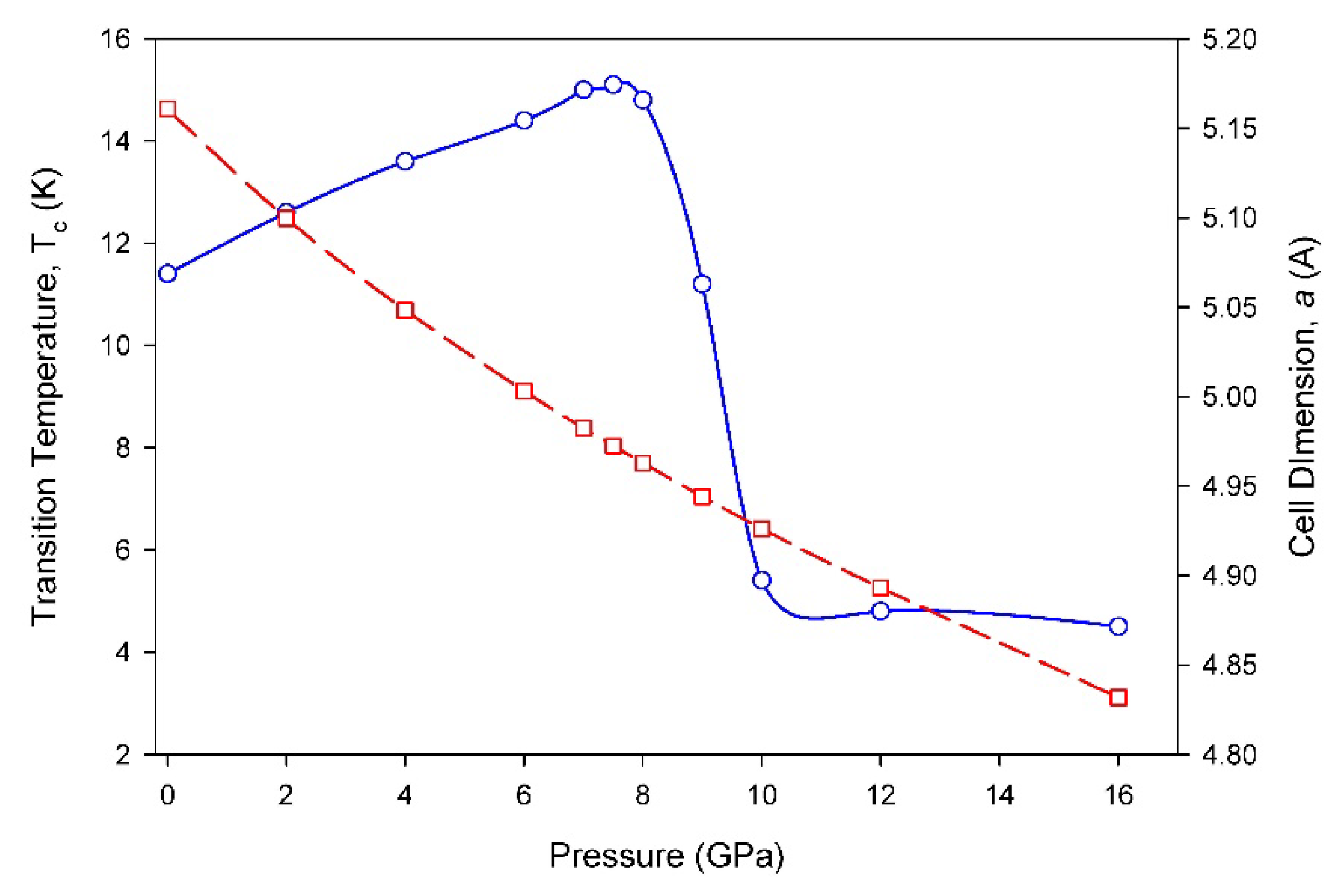
Figure S4 (Supplemental) shows band structure calculations for two other pressures - 4 GPa and 12 GPa - to delineate trends in this modelling approach. We show in Figure 3 that at a pressure of 7.5 GPa, the non-bonding-point, Ec*/2 is near the Fermi level (at 22.8 meV). The position of the bonding to antibonding crossing at this pressure corresponds to the highest experimentally determined Tc for CaC6 as shown in Figure 5 (extracted and adapted from ref [36]). As shown in Figure S4, the cosine band crosses the Fermi level with different proportions of bonding and antibonding character depending on the external pressure. This relative shift in bonding-antibonding character is also consistent with the changes in Tc observed with pressure.
As discussed in detail below, to determine the superconducting gap, the tight binding gap ETB Gap@Γ (the highest asymmetry offset) must be corrected by a factor determined by the fraction of the Fermi surface that participates in unencumbered, or non-interfering, nesting between open loops. If other Fermi surface bands cross the nested region, or the Fermi surface curvature deviates substantially, a different nesting vector is required. In such a case, additional phonons of different energy/frequency must become involved for conservation of energy and momentum. In this case, coupling between electrons at opposite sides of the Fermi surface, requiring additional phonons, translate into the equivalent of scattering events.
Figure 5.
Graph of the experimentally determined superconducting transition temperature for CaC6 as function of pressure (re-plotted and adapted from reference [37]). The rhombohedral cell dimension, a, as function of pressure is also plotted.
Figure 5.
Graph of the experimentally determined superconducting transition temperature for CaC6 as function of pressure (re-plotted and adapted from reference [37]). The rhombohedral cell dimension, a, as function of pressure is also plotted.
3.5. Superlattice Nesting Vectors and Key Phonon Wavevectors
The rhombohedral and hexagonal reciprocal unit cells for CaC6 are related by the following equations:
ΓZR = 3ΓAH
ΓZR = π/c
c =13.572 Å
(a1* + a2* + a3*)/3 = π/c
Thus, twice the ΓAH distance of the reciprocal hexagonal unit cell (2π/3c), and half of this reciprocal distance (π/3c = 2π/6c), correspond to distances between Brillouin zone (BZ) boundaries or between the Γ-point and the BZ boundary for the 2c-real space hexagonal superlattice. For Fermi surface features, this real space superlattice corresponds to a repeat distance of a folded hexagonal supercell in reciprocal space.
This reciprocal space vector and related dimensional relationships to the primitive rhombohedral cell, are particularly useful for understanding crystallographic relationships in the CaC6 structure. For example, the reciprocal space vector is itself a ‘nesting’ vector in the perpendicular c or c*-direction for Fermi surfaces of the CaC6 2c superlattice as shown in Figure 6a. This nesting vector joins significant proportions of the folded Fermi surfaces and can be considered a vertical component of diagonal nesting vectors [18].
The extent of diagonal nesting vectors is clear in MgB2 [18], which has a cosine shaped Fermi surface profile. For MgB2, nesting by parallel reciprocal vectors of identical magnitude spans the entire warped tubular Fermi surfaces of MgB2 [18]. The same condition cannot be said for CaC6.
In CaC6, the approximately circular profiles of Fermi surface cross-sections significantly reduce the extent of nesting, although nesting conditions do not require existence over the entire Fermi surface [32]. Consequently, for CaC6 the nesting extent is difficult to determine accurately with comparable error or uncertainty to that followed for MgB2 [18]. Another source of error is the thermal energy width (~kBT) that occurs around the Fermi surface at temperatures above absolute zero. The width of this thermal energy nominally extends the region by ~1.4meV at 16K where nesting by the same original phonon vector is maintained.
Figure 6 shows cross-sections of the Ca-4s dominated Fermi surfaces for CaC6 at selected pressures. In Figure 6, green- and orange-coloured circles delineate the contours of Fermi surfaces, as well as indicate a change in phase introduced by folding on the alternating (approximate) spherical Fermi surfaces. Note that changes in phase between bonding and antibonding regions for the same Fermi surfaces exist as indicated by the phase of the cosine functions themselves, where the plane perpendicular to ΓZ at the mid-point Z/2 defines the transition boundary between bonding and antibonding behaviours (see Supplementary Figure S5). Therefore, the folded Fermi surfaces require a careful identification of phase variation, which may be complex and/or convoluted and so, are difficult to track and represent graphically.
In Figure 6, blue lines that are parallel to the nesting vectors and of the same magnitude, do not connect the Fermi surface regions. Thus, the extent of nesting is limited to a window around the ‘crossing’ of Fermi surfaces (joined by red and purple lines that cross the centre of the double stacked Brillouin zones). The brown arrows (circled) in the inset of Figure 6a correspond to the maximum electron momentum transfer between y and z directions (~ΓK/15) that are coherently accommodated through nesting by a phonon of appropriate frequency for energy conservation.
At 0 GPa, both red and orange vectors produce a nesting relationship that crosses the Γ point centre at the midpoint. The diagonal nesting relationships have vectors qD and qd (in Figure 6a, D and d stand for long and short diagonals, respectively, where qD = 3qd) with projections approximately given by:
qD = 2ΓK/3 ± ΓAH = 2ΓK/3 ± (π/3c) kz
qd = qD/3 = 2ΓK/9 ± ΓAH/3 = 2ΓK/9 ± (π/9c) kz
The nesting vectors connect open loops with kF and -kF at opposite sides through the origin. Thus, these nesting vectors connect bonding and antibonding branches of the relevant band, and are associated with Cooper-pairing [18]. In this case, the nesting vector corresponds to the primary phonon in electron-phonon coupling by the relationships:
-kF1 + qD,d = kF1’
-kF2 - qD,d = kF2’
At 7.5 GPa, the diagonal nesting relationships have vectors qD and qd (in Figure 6c, where qD = 2qd) with projections approximately given by:
qD = 4ΓK/11 ± ΓAH = 4ΓK/11 ± (π/3c) kz
qd = qD/2 = 2ΓK/11 ± ΓAH/2 = 2ΓK/11 ± (π/6c) kz
3.5.1. Coherent Electron-Phonon Coupling via Acoustic Nesting
As schematically shown in Figure 6a–c, nesting between mid-points in different Brillouin zones establishes favourable reference points for an electron–phonon coupling condition between opposite sides of the Fermi surface. These points are non-bonding and establish a reference for phase relationships. However, the coherence of electrons coupled by this same nesting phonon vector only survives without disturbance while intersection with any new Fermi surface associated with a different band of unrelated symmetry is absent. Coherent coupling is also lost when the curvature of the Fermi surfaces changes such that a nesting vector of fixed magnitude does not link electron states on opposite sides of the Fermi surface. For CaC6, examples of this loss of connectivity by nesting vectors on opposite sides of the Fermi surface are shown as blue (dotted) arrows in Figure 6a–c.
Figure 6 also enables identification of two general types of nesting. These two types are:
Closed loops alone do not appear to be conducive to superconductivity but may be indirectly involved in superconducting behaviour. However, for this CaC6 system, open loops are continuously connected in the extended Brillouin zone scheme. Thus, open loops correlate with superconductivity through the magnitude of nesting vectors and the extent of nested regions. In Figure 6a, the purple-coloured vectors run parallel to the red and orange arrows but are shorter in length. By comparing these vectors at pressures of 0 GPa and 7.5 GPa, we can identify other features including density of states. In Figure 6a–c, the purple-coloured vectors are approximately one third and one half of the red nesting vectors, respectively. This relationship suggests that the shorter purple vectors are nesting vectors themselves, and given their multiplicity, are indicators of the relative population of density of states.
The proportions of a Fermi surface that participate, and remain with, a given acoustic nesting vector, defines a proportion of the cosine amplitude that remains coherently coupled. This fraction, multiplied by the above mentioned tight binding gap, ETB Gap@Γ, provides an accurate estimate of the superconducting gap (provided DFT calculations are carried out with sufficient resolution [23]).
The superconducting TB gap value at 0 GPa is the ETB Gap@Γ value at Γ divided by 3, because of the three parallel nesting vectors that fit between nested Fermi surface spheres, multiplied by the fraction of the folded z*-axis that is nested; which is ~ 0.55 (see Figure 6a). The superconducting TB gap value at 7.5 GPa is the value at Γ divided by 2, because there are two parallel nesting vectors that fit between nested Fermi surface spheres, multiplied by the fraction of the folded z*-axis that is nested; which is ~ 0.43 (see Figure 6c).
The superconducting TB gap value at 4 GPa is obtained by linearly extrapolating the number of parallel nesting vectors that fit between nested Fermi surface spheres, times the linear extrapolation of the fraction of the folded z*-axis that is nested. These extrapolations result in 3.21+ (5.49 -3.21) x (4/7.5) = 4.43, 0.55 – (0.55-0.43) x (4/7.5) = 0.486, and 4.43 x 0.486 = 2.15 for (i) the parallel nesting vectors, (ii) the fraction of z*-axis that can be nested and (iii) the superconducting TB gap, respectively (see Table S1, Supplemental). We estimate the error in determining the superconducting TB gap at ±0.09 meV. Values of the calculated gaps for other pressures are given in Table S1.
If we include the additional periodicity identified in Section 3.2 from the cosine dependence of the average of bonding and antibonding energies, we obtain a 4c superlattice symmetry. This superlattice symmetry introduces an extra folding in reciprocal space at π/4c. This additional folding more accurately reflects the dynamic symmetry of the structure, compared to calculations without additional folding. We suggest that calculations in which the full z*-axis participates in nesting are more likely to effectively represent coherent superconducting transport behaviour. In addition, this additional folding brings the non-bonding, cosine inflection points to the Γ direction. This condition is, intuitively, an appropriate locus for electron phonon coupling, that initiates the exchange of sound velocity between y and z-directions, as electrons travel the cosine bands or the corresponding Fermi surface.
The highest Tc is obtained when the Fermi level and the non-bonding energy of the cosine shaped band coincide. This represents the most balanced distribution between fully occupied bonding states and fully unoccupied antibonding states. This configuration suggests that the optimal conditions for superconductivity occur when the smallest energy is needed for the excitation of electrons in filled bonding states into empty antibonding states, and that this energy, translated for interactions between quasiparticles, corresponds to the superconducting gap.
3.6. Phonon Frequencies and the Superconducting Gap Energy
This section focuses on the 0 GPa case with similar extension to DFT calculations for CaC6 under higher pressure conditions. The difference in phonon vectors for conserved momentum transfers in the y- and z-directions of the nested regions are approximately ΓK/15 and 3ΓK/10 (= (9/2) ΓK/15); and ΓAH and ΓAH/3, respectively, as shown in the inset of Figure 6a.
Figure S6 (Supplemental) displays the phonon dispersion (PD) for CaC6 with Ca isotope 40, calculated using the LDA functional and k-grid Δk=0.015 Å-1, with CASTEP Materials Studio 2023 software. A PD for CaC6 with Ca isotope 44 is also provided in the Supplemental section (Figure S6).
Figure S6 (Supplemental) shows that all phonon vectors associated with nesting (ΓK/15, 3ΓK/10, ΓAH and ΓAH/3) have values on acoustic phonon dispersion (PD) branches with similar energy at 39.6cm-1 (i.e., 4.91 meV). These acoustic energies (or multiples of energy depending on degeneracy or multiplicity) accompanying the nested momentum transfers must be exchanged (absorbed or provided) in an electron-phonon coupling, for coupled electron movement along the nested regions on either side of the Fermi surface to conserve energy and to remain coherent [18].
These calculations of PDs for CaC6 using the hexagonal unit cell shown in Figure 4 are consistent with calculated PDs for CaC6 using the rhombohedral cell by Calandra and Mauri [38]. The latter give values of frequency for the equivalent of ~ ΓM/15 and ΓK/15 that closely match half the energy of asymmetry in the cosine function (i.e., the tight binding gap) at Γ as listed in Table S1 for LDA (i.e. 10.3/2 meV = 5.15 meV, although depending on pseudopotential, values as low as 9.8/2 = 4.9 meV are obtained). In Figure S5, the frequency of 39.6 cm-1 is ~ 4.91 meV (= 3 x 1.63 meV), or approximately three times the superconducting gap energy [36,39] at 0 GPa. Thus, we show there is a clear geometrical origin for phonons engaged in the conservation of energy with electrons coupled via these nesting relationships.
The rhombohedral calculations by Calandra and Mauri [38] also show that:
or, alternatively, from our hexagonal calculations:
ωL(ΓZ/6) = ωT(ΓZ/2) ≈ ωT(ΓT/2)
ωL(ΓA/3) = ωT(ΓA) ≈ ωT, L(ΓK/15) = ωT(3ΓK/10)
These equivalences suggest that inter-conversion of transverse phonons into longitudinal phonons, and vice versa, by addition and subtraction is highly probable. Similarly, longitudinal and transverse vibrations in the kx ky-plane may convert to the transverse and longitudinal vibrations in the kz-direction, respectively [23]. This interaction favours energy conversion between different acoustic phonon branches and perhaps enhances the creation of optical phonons; the latter may also be required to maintain coherency.
3.6.1. The Isotope Effect for CaC6
Employing the McMillan formula [40], the critical transition temperature for 40Ca computed by Calandra and Mauri, [38] aligned well with experimental data. Notably, the calculated isotope effect for 44Ca relative to 40Ca differed by 0.24 K. This value contrasts with experimental observation of a larger isotope effect, of ~ 0.5 K difference in Tc reported by Hinks et al. [41].
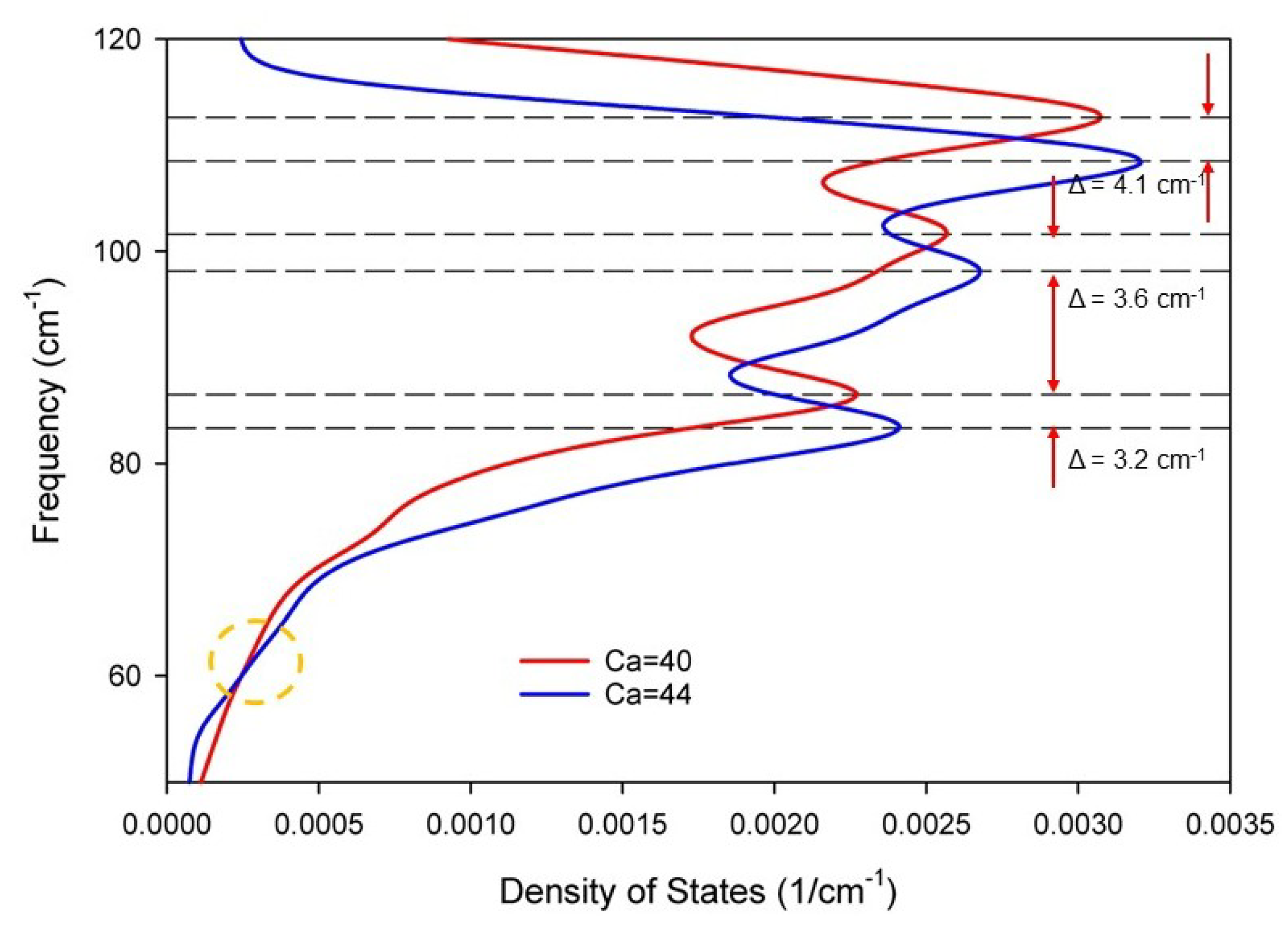
Figure 7 shows an overlay of the phonon dispersions (PD’s) calculated for a single hexagonal unit cell of CaC6 using the two most abundant isotopes of Ca, namely 40Ca and 44Ca. Figure 7b is an enlarged view of the acoustic region in the ΓA-direction highlighted by the orange rectangle in Figure 7a. Figure 8 shows the low frequency region of the phonon density of states (PDOS) calculated for a single hexagonal unit cell of CaC6 also using 40Ca and 44Ca. The PDOS for the full frequency range is given in supplementary Figure S7. The reference lines are guides to the eye for relative changes in frequency (or energy) with colours matching the respective isotopes.
The difference in acoustic frequencies at the Brillouin zone boundary, A, is 3.0 ± 0.4 cm-1 (=0.37 ± 0.05 meV). For the midpoint A/2, which corresponds to the Brillouin zone boundary of the folded reciprocal space of the 2c superlattice, ~ 1.5 cm-1 (=0.18 meV). Therefore, if the isotope effect is predominantly controlled by acoustic frequencies, the change in Tc for the isotope effect should be proportional to the frequency difference at the Brillouin zone boundaries of the 2c superlattice for the same nesting phonon vector. We assume that the frequency 39.6 cm-1 is proportional to the experimentally determined Tc of 11.4K (see Figure 5 and Section 3.4), then 1.5 cm-1 corresponds to 11.4K x (1.5/39.6) = 0.43 ± 0.06 K. This calculated value for the difference in Tc for Ca isotopes is in close agreement with the experimentally measured isotope shift determined by Hinks et al. [41].
Comparing the PDOS for Ca isotopes (see Figure 8 and supplementary Figure S7), a change to their relative position occurs at ~ 60 cm-1 (see dotted circle in Figure 8). The first PDOS peak at low frequency, shows a frequency difference in the 40Ca and 44Ca peak positions that exceeds the calculated value determined above for the isotope effect using PDs. Moreover, the difference in peak positions increases as the calculated frequencies approach the range of optical phonons. This variation in peak positions suggests that Tc estimates based on density of states calculations will be inaccurate, particularly at higher frequencies than acoustic. This inaccuracy may account for a limited success with the accuracy of McMillan equations and similar approaches, particularly for complex compounds. For calculated PDs of complex compounds, some optical modes may contribute non-linearities to the dispersion. As stated by Jones and March [42], densities of states are a conceptual compromise when full PD and EBS calculations are not available.
4. Conclusions
We have used a systematic approach to DFT modelling that enables extraction of superconductivity parameters from band structure and phonon dispersion calculations (requiring fine k-grid and large cut-off radius for meV resolution). This approach is extended to CaC6 for which superlattice constructs, motivated by experimental observations, are consistent with cosine shaped band structures along the layer direction. Interrogation of Fermi surfaces reveal important bonding-antibonding and nesting relationships that display an asymmetry with a strong connection to superconductivity and identification of a superconductivity gap. The extent and nature of this asymmetry, evidenced in band structures and Fermi surface projections, aligns with the experimentally determined change in Tc with applied pressure. These results demonstrate that superconductivity is largely a geometrically tuned phenomenon, implicit in observations of superconductivity in many different crystal structures of widely varying geometry. We have shown that accurate and mechanistic information on superconductivity can be extracted from an analytical interrogation of EBS, Fermi surface and PD calculations. Superlattice constructs, supported by extensive experimental observations of their manifestation, for example via Raman and THz spectroscopy, are useful tools for understanding this important phenomenon.
Supplementary Materials
The following supporting information can be downloaded at the website of this paper posted on Preprints.org, Figures S1–S3: Calculated EBS for CaC6 with rhombohedral and hexagonal cells; Figure S4: Calculated EBS for CaC6 with 2c hexagonal cells at 0 GPa and 7.5 GPa; Figure S5: Schematic of the CaC6 Fermi Surface; Figure S6: Calculated phonon dispersions for 40CaC6 and 44CaC6; Figure S7: Calculated phonon density of states for 40CaC6 and 44CaC6; Table S1: Summary calculated parameters for CaC6.
Author Contributions
Conceptualization, J.A. and I.M.; methodology, B.W., A.B. and J.A.; software, W.B. and J.A.; validation, J.A., I.M. and A.B.; formal analysis, A.B. and J.A.; investigation, W.B.; resources, J.A.; writing—original draft preparation, W.B. and J.A.; writing—review and editing, J.A. and I.M.; visualization, I.M. and J.A.; supervision, J.A. All authors have read and agreed to the published version of the manuscript.
Funding
This research received no external funding.
Data Availability Statement
The raw data supporting the conclusions of this article will be made available by the authors on request.
Acknowledgments
The authors are grateful to the e-Research Office at QUT for access to high-performance computing (HPC) and assistance, and to QUT for a scholarship award to BW. The authors also thankful for access to Bunya HPC facilities and ongoing assistance from Dr. Marlies Hankel at UQ.
Conflicts of Interest
The authors declare no conflict of interest.
References
- James Patterson, B. Bailey, Solid-State Physics: Introduction to the Theory, Second ed., Springer-Verlag Berlin Heidelberg Germany 2010.
- Ferreira, R., Chapter 1: Introduction to Semiconductor Heterostructures, in: Xavier Mari, N. Balkan (Eds.), Semiconductor Modelling Techniques, Springer-Verlag Berlin Heidelberg Germany, 2012.
- Ivchenko, E.L., G.E. Pikus, Superlattices and Other Heterostructures: Symmetry and Optical Phenomena, Second ed., Springer-Verlag 1997.
- He, F., Zhou, Z. Ye, et al., Moiré patterns in 2D materials: a review, ACS Nano 15 (2021) 5944-5958.
- Li, Z., J.M. Lai, J. Zhang, Review of phonons in moiré superlattices, Journal of Semiconductors 44 (2023).
- Li, Y., Wan, N. Xu, Recent Advances in Moiré Superlattice Systems by Angle-Resolved Photoemission Spectroscopy, Advanced Materials (2023).
- Mangold, M.A., A.W. Holleitner, J.S. Agustsson, M. Calame, Nanoparticle Arrays, in: Aliofkhazraei, M. (Ed.), Handbook of Nanoparticles, Springer2016.
- Cargnello, M., A.C. Johnston-Peck, B.T. Diroll, et al., Substitutional doping in nanocrystal superlattices, Nature 524 (2015) 450-+.
- Yazdani, N.. M. Jansen, D. Bozyigit, et al., Nanocrystal superlattices as phonon-engineered solids and acoustic metamaterials, Nature Communications 10 (2019).
- Logvenov, G., N. Bonmassar, G. Christiani, et al., The Superconducting Dome in Artificial High-Tc Superlattices Tuned at the Fano–Feshbach Resonance by Quantum Design, Condensed Matter 8 (2023) 78-84.
- Bianconi, A., Feshbach shape resonance in multiband superconductivity in heterostructures., J. Supercond.: Incorporating Novel Magnetism 18 (2005) 626-636.
- Bianconi, A., A. Valletta, A. Perali, N.L. Saini, High Tc superconductivity in a superlattice of quantum stripes, Solid State Communications 102 (1997) 369-374.
- Bianconi, A., D. Di Castro, S. Agrestini, et al., A superconductor made by a metal heterostructure at the atomic limit tuned at the 'shape resonance': MgB2, Journal of Physics-Condensed Matter 13 (2001) 7383-7390.
- Sboychakov, A.O., K.I. Kugel, A. Bianconi, Moiré-like Superlattice Generated van Hove Singularities in a Strained CuO2 Double Layer, Condensed Matter 7 (2022) 50-59.
- Alarco, J.A., B. Gupta, M. Shahbazi, et al., THz/Far infrared synchrotron observations of superlattice frequencies in MgB2, Phys. Chem. Chem. Phys. 23 (2021) 23922-23932.
- Alarco, J.A., A. Chou, P.C. Talbot, I.D.R. Mackinnon, Phonon Modes of MgB2: Super-lattice Structures and Spectral Response, Phys. Chem. Chem. Phys. 16 (2014) 24443-24456.
- Alarco, J.A., I.D.R. Mackinnon, Phonon dispersions as indicators of dynamic symmetry reduction in superconductors, in: Stavrou, V.N. (Ed.), Phonons in Low Dimensional Structures, InTech Open, London UK, 2018, pp. 75-101.
- Alarco, J.A., I.D.R. Mackinnon, Superlattices, Bonding-Antibonding, Fermi Surface Nesting, and Superconductivity, Condensed Matter, 2023.
- Emery, N., C. Hérold, M. d’Astuto, et al., Superconductivity of Bulk CaC6, Physical Review Letters 95 (2005) 087003.
- Weller, T.E., M. Ellerby, S.S. Saxena, et al., Superconductivity in the intercalated graphite compounds C6Yb and C6Ca, Nature Physics 1 (2005) 39-41.
- Giannozzi, P., S. Baroni, N. Bonini, et al., QUANTUM ESPRESSO: a modular and open-source software project for quantum simulations of materials, Journal of Physics: Condensed Matter 21 (2009) 395502.
- Clark, S.J., M.D. Segall, C.J. Pickard, et al., First principles methods using CASTEP, 220 (2005) 567-570.
- Mackinnon, I.D.R., Almutairi A., J.A. Alarco, Insights from systematic DFT calculations on superconductors, in: Arcos, J.M.V. (Ed.), Real Perspectives of Fourier Transforms and Current Developments in Superconductivity, IntechOpen Ltd., London UK, 2021, pp. 1-29.
- Bartók, A.P., J.R. Yates, Ultrasoft pseudopotentials with kinetic energy density support: Implementing the Tran-Blaha potential, Physical Review B 99 (2019) 235103. [CrossRef]
- Perdew, J.P., K. Burke, M. Ernzerhof, Generalized Gradient Approximation Made Simple, Physical Review Letters 77 (1996) 3865-3868.
- Perdew, J.P., J.A. Chevary, S.H. Vosko, et al., Atoms, molecules, solids, and surfaces: Applications of the generalized gradient approximation for exchange and correlation, Physical Review B 46 (1992) 6671-6687. [CrossRef]
- Alarco, J.A., P.C. Talbot, I.D.R. Mackinnon, Comparison of functionals for metal hexaboride band structure calculations, Mod. Numer. Sim. Mater. Sci. 4 (2014) 53-69.
- Alarco, J.A., M. Shahbazi, P.C. Talbot, I.D.R. Mackinnon, Spectroscopy of metal hexaborides: Phonon dispersion models, J. Raman Spect. 49 (2018) 1985-1998. [CrossRef]
- Klingshirn, C.F., C.F. Klingshirn, Crystals, Lattices, Lattice Vibrations and Phonons, Semiconductor Optics (2102) 135-166.
- Deymier, P.A., Acoustic metamaterials and phononic crystals, Springer Science & Business Media2013.
- Csányi, G., P.B. Littlewood, A.H. Nevidomskyy, The role of the interlayer state in the electronic structure of superconducting graphite intercalated compounds, Nature Physics 1 (2005) 42-45. [CrossRef]
- Grüner, G., Density waves in solids, 1994.
- Ferry, D.K., Semiconductors: Bonds and bands, IoP Publishing2019.
- Huebener, R.P., Conductors, semiconductors, superconductors, Springer International Publishing2019.
- Canadell, E., M.-L. Doublet, C. Lung, Orbital Approach to the Electronic Structure of Solids, Oxford University Press, Oxford, UK, 2012.
- Gauzzi, A., S. Takashima, N. Takeshita, et al., Enhancement of superconductivity and evidence of structural instability in intercalated graphite CaC6 under high pressure, Physical Review Letters 98 (2007).
- Gauzzi, A., S. Takashima, N. Takeshita, et al., Enhancement of Superconductivity and Evidence of Structural Instability in Intercalated Graphite CaC6 under High Pressure, Physical Review Letters 98 (2007) 067002. [CrossRef]
- Calandra, M., F. Mauri, Theoretical Explanation of Superconductivity in CaC6, Physical Review Letters 95 (2005) 237002.
- Gonnelli, R.S., D. Daghero, D. Delaude, Evidence for Gap Anisotropy in CaC6 from Directional Point-Contact Spectroscopy, Physical Review Letters 100 (2008).
- McMillan, W.L., Transition Temperature of Strong-Coupled Superconductors, Physical Review 167 (1968) 331-344.
- Hinks, D.G., D. Rosenmann, H. Claus, et al., Large Ca isotope effect in the CaC6 superconductor, Physical Review B 75 (2007) 014509.
- Jones, W., N.H. March, Theoretical solid state physics, Courier Corporation1985.
Figure 1.
Schematic of a chain of atoms with s-orbitals (e.g. a chain of H-atoms) in the bonding (bottom of a cosine band) and anti-bonding (top of a cosine band) orbital configurations. Grey circles represent combined orbital designations.
Figure 1.
Schematic of a chain of atoms with s-orbitals (e.g. a chain of H-atoms) in the bonding (bottom of a cosine band) and anti-bonding (top of a cosine band) orbital configurations. Grey circles represent combined orbital designations.
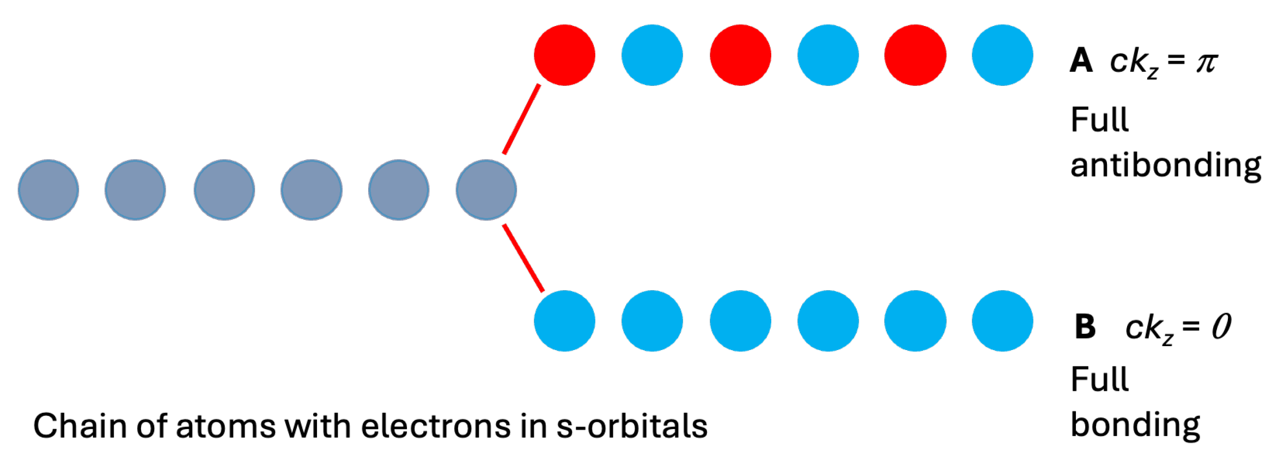
Figure 2.
Electronic band structures of CaC6 at 0 GPa (Space Group R-3m) calculated for: (a) rhombohedral symmetry and (b) equivalent hexagonal symmetry. The cosine-shaped interlayer band along the c* direction crosses the Fermi level (dotted horizontal line) in both cases. In (a) the energy, Ec*/2, is -193.5 meV and the average energy, Eav, between antibonding (A) and bonding (B) nodes of the cosine band is -150.0 meV. This energy difference, ΔE, reflects the marginal asymmetry of the cosine band. In (b) the same cosine band is folded in the hexagonal configuration and results in two bonding (B, Bʹ) and two antibonding (A, Aʹ) nodes of the cosine band. Similarly, Eav and Eʹav show different energy values to Ec*/2 with a net ΔE of 43.4 meV (at higher magnification in the inset). EBS plots showing conventional reciprocal directions and the location of the cosine band are provided in Supplemental Figures S1–S3.
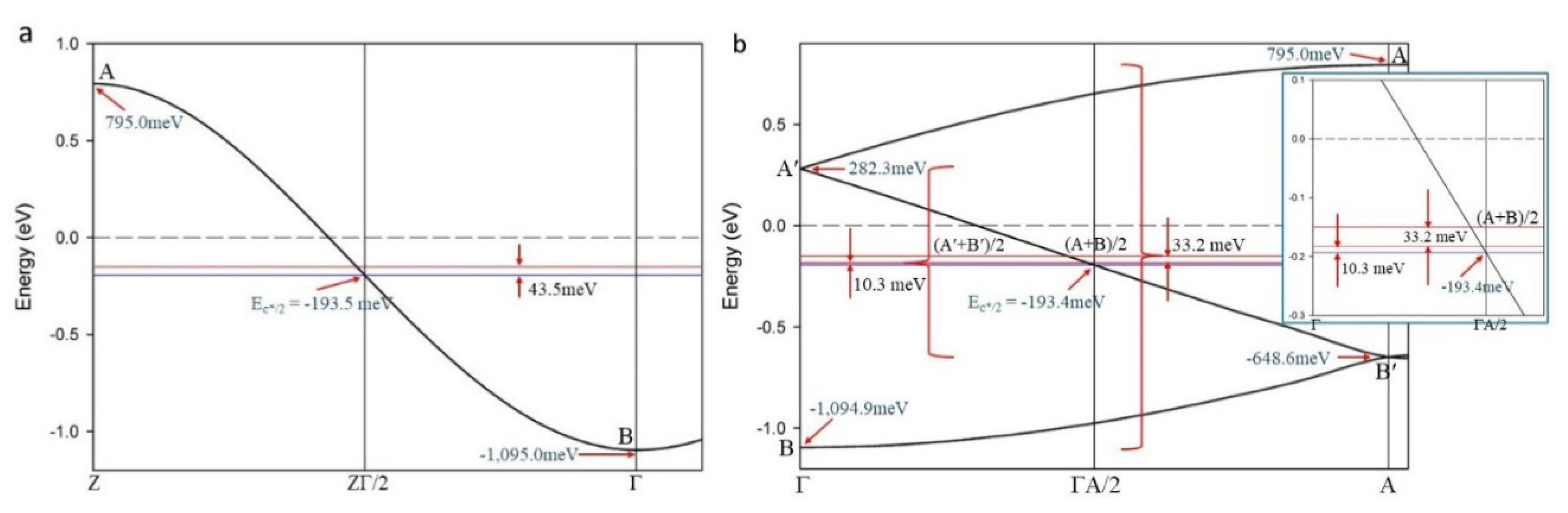
Figure 3.
Electronic band structures of CaC6 (Space Group R-3m) calculated for a 2c hexagonal lattice: (a) at 0 GPa and (b) at 7.5 GPa. In both cases, the folded cosine-shaped interlayer band along the c* direction crosses the Fermi level (dotted horizontal line). In (a) the energy, Ec*/2, is -198.5 meV and is at the intersection on Z where the two branches of the cosine curve from Aʹ and Bʹ meet. The net energy difference, ΔE, is 43.5 meV. This energy difference, ΔE, reflects the marginal asymmetry of the cosine band for a 2c superlattice at 0 GPa. The calculation for CaC6 at 7.5 GPa, shows a shift of the folded bands along c* towards higher energy, with Ec*/2 above the Fermi level at 22.8 meV. In addition, the net ΔE value is 50.7 meV, an increase of 7.2 meV compared to 0 GPa.
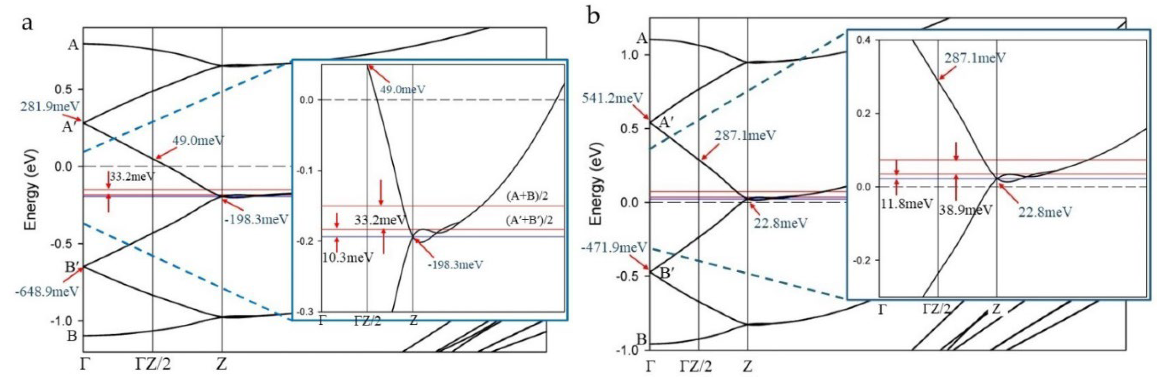
Figure 4.
Enlarged view of the electronic band structure of CaC6 at 0 GPa calculated for rhombohedral symmetry and folded at the midpoint ΓZ/2. The average energy Eav = ½(A+B) at Γ is plotted as the red line. Eav = ½ (A+B) as function ofkz is plotted as the dark continuous line between Eav and Ec*/2 (blue line) with a cosine shape and a full period of π/c.
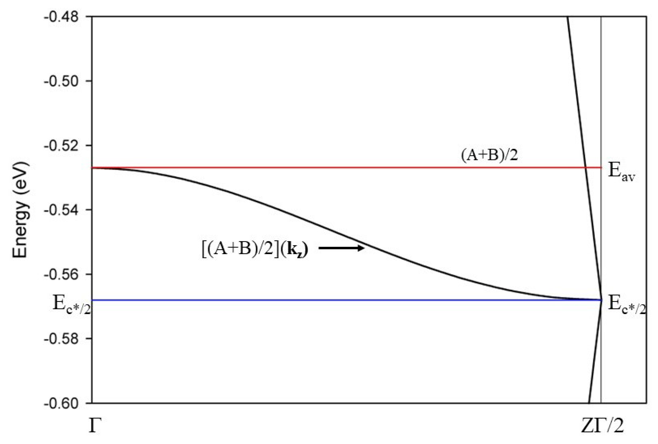
Figure 6.
Cross-sectional views of the Ca-4s Fermi surfaces for CaC6, calculated for 2c hexagonal supercells at pressures: (a) 0 GPa, with detailed view of the Fermi surface crossing point (inset), (b) 4 GPa and (c) 7.5 GPa. Two of the first Brillouin zone sections along the c* reciprocal direction are displayed. Contours for the Fermi surfaces are green- and orange-coloured lines. Nesting vectors of identical length that join opposite sides of the Fermi surface, parallel to the vector that crosses the centre point or origin (A), are shown in red, orange, and purple arrows. See text for further details.
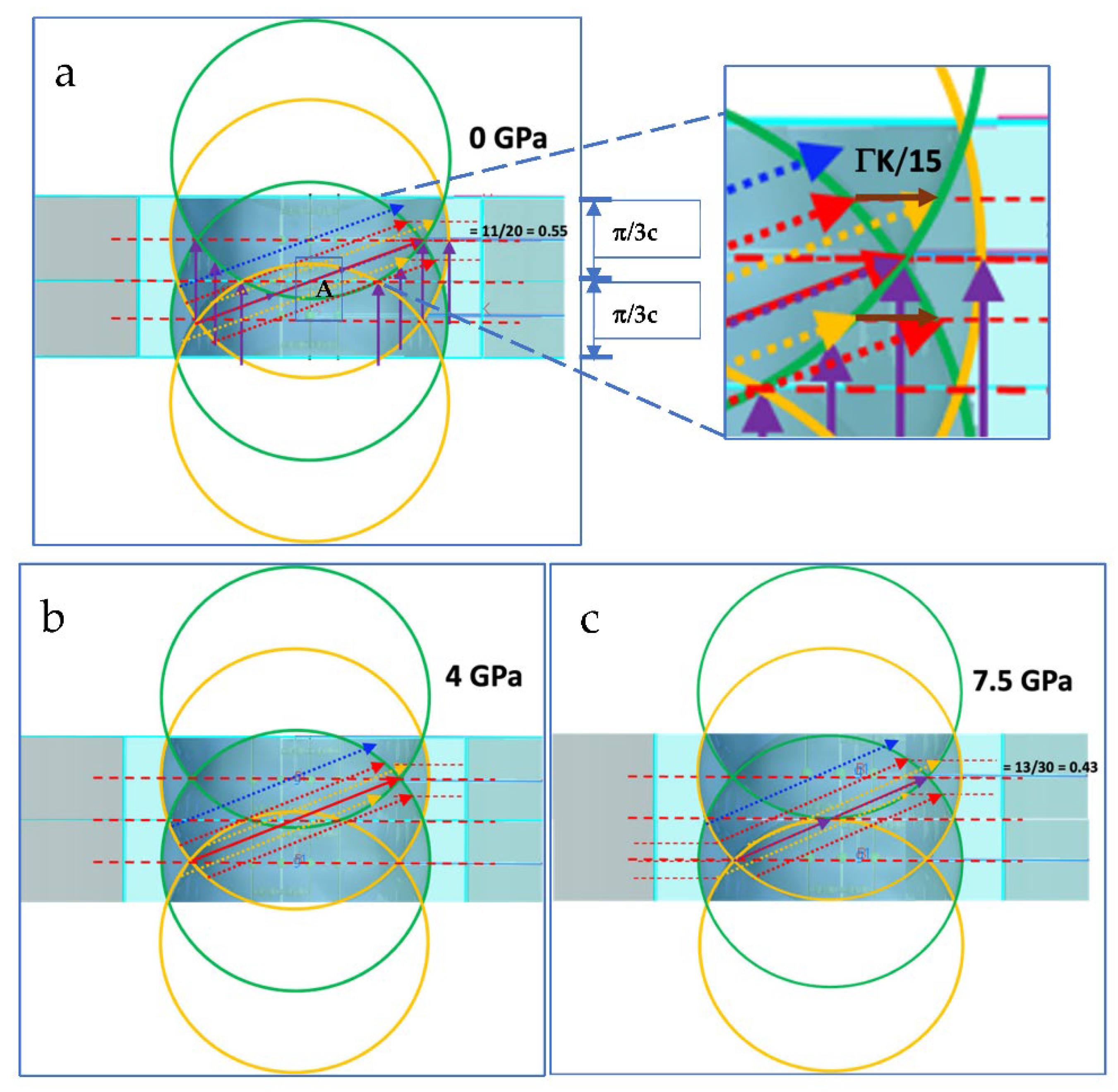
Figure 7.
(a) Phonon dispersion (PD) for CaC6 calculated with a hexagonal unit cell using DFT with LDA functional and k-grid value 0.015Å-1. The PD in red is calculated for 40Ca and the PD in blue for 44Ca isotope, respectively. (b) Magnification of the orange rectangle in (a), showing differences in frequency (Δω = 3.0 ± 0.4 cm-1) between both isotopes at reciprocal point A.
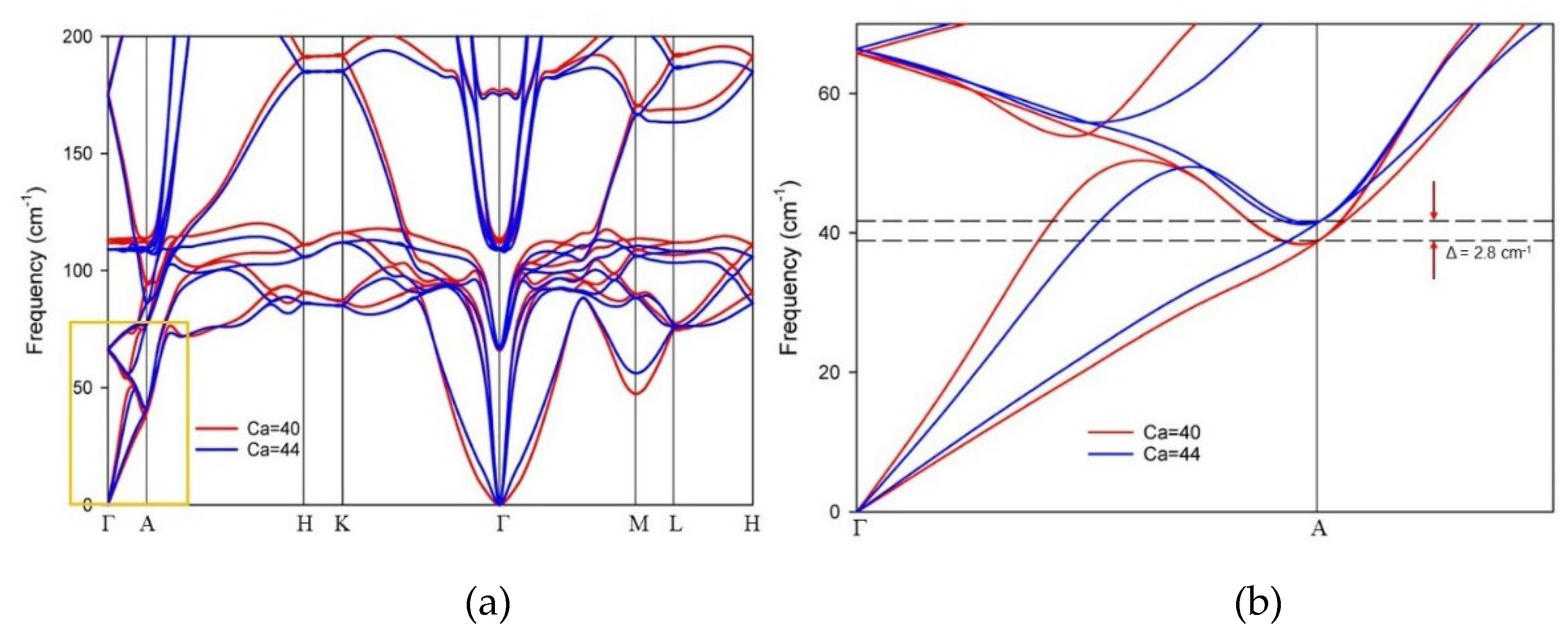
Figure 8.
Phonon Density of States (PDOS) for 40Ca and for 44Ca isotopes, showing relative shifts in peak density (and differences in frequency, Δω) with increase in phonon frequency.
Figure 8.
Phonon Density of States (PDOS) for 40Ca and for 44Ca isotopes, showing relative shifts in peak density (and differences in frequency, Δω) with increase in phonon frequency.
Disclaimer/Publisher’s Note: The statements, opinions and data contained in all publications are solely those of the individual author(s) and contributor(s) and not of MDPI and/or the editor(s). MDPI and/or the editor(s) disclaim responsibility for any injury to people or property resulting from any ideas, methods, instructions or products referred to in the content. |
© 2024 by the authors. Licensee MDPI, Basel, Switzerland. This article is an open access article distributed under the terms and conditions of the Creative Commons Attribution (CC BY) license (http://creativecommons.org/licenses/by/4.0/).
Copyright: This open access article is published under a Creative Commons CC BY 4.0 license, which permit the free download, distribution, and reuse, provided that the author and preprint are cited in any reuse.


