Submitted:
19 April 2024
Posted:
22 April 2024
You are already at the latest version
Abstract
Karst peaks and depressions are scattered in karst zones with strong spatial heterogeneity and fragile ecological environments and are crucial for determining the degree of karst geomorphologic development. However, realizing automatic depiction and extracting depressions with high accuracy is difficult because of their complex morphology. Herein, based on 12.5-m resolution DEM data, six typical karst peaks from depressions in southwest China were selected as the study areas and a revised terrain openness index method based on slope mutation points (ROBSMPs) was used to determine the degree of karst geomorphologic development and the boundary of karst depressions. The extent of depressions extracted by ROBSMPs and the terrain openness index method with the extent of depressions hand-drawn based on remote sensing images was compared and analyzed. The results show that compared with the topographic openness index method, the overall accuracy of karst depression extracted by ROBSMPs was improved and the perimeter, area, and raster displacement error indexes were reduced. ROBSMPs realized high-precision extraction of depressions, thereby strengthening the applicability of the topographic openness index method to karst peak zones. This study offers a new perspective and path toward the expansion of digital terrain analysis technology in karst mountainous areas and is expected to play a vital role in the extraction of similar geomorphic units in karst zones.
Keywords:
topographic openness index method
; slope
; karst
; depressions
1. Introduction
The global concentrated and continuous distribution of karst zones primarily includes three large areas: south-central Europe, eastern North America, and southwestern China. Southwestern China has the largest continuous distribution of karst area, the largest concentration of population, and enriched karst development [1]. The combination of peaks and depressions within southwestern China reflects the development maturity of karst geomorphology and is unique to China [2,3]. Depressions in combined karst peak–depression terrain areas (hereinafter, karst peak zones) is used as a general term for various types of closed negative terrains formed by karst effect in carbonated rock areas [4,5]. These depressions are a result of the confluence of water flow, where energy and transported material are concentrated and accumulated due to the dissolving and eroding actions of various forms of water flow [6]. Moreover, they represent the most valuable but limited agricultural and construction land in the region. Using high-precision topographic data to reasonably divide peaks and depressions and detect karst depressions can help to study theories of karst generation conditions and the development and evolution of karst landforms with respect to the roles of geology, climate, hydrology, and biology in karst peak zones; deepen the understanding of the development of karst landforms; and provide references for national land space planning and ecological civilization construction in karst areas.
Currently, the main methods for detecting depressions in karst peak zones can be classified into four categories. First is the contour method, in which depressions are detected from contoured terrains [7,8,9,10]; however, the detected depressions often form a peak–depression combination, whereby neighboring peaks are classified as the same terrain unit, making it difficult to determine the exact extent of the depression. Second is the hydrological analysis method; this method involves the use of the ArcGIS software hydrological analysis module and a digital elevation model (DEM) to perform a filling process to identify and detect depressions [11,12,13,14,15]. However, the area to which this process can be applied is limited and the number of detected depressions is small; therefore, some depressions are missed. Third is the saddle point spatial interpolation method, whereby detected saddle points are spatially interpolated and subtracted from a DEM to obtain a range of depressions [17]. However, when detecting depressions using this method, the spatial closure of the depressions is not fully considered and there is a gap between the detected depressions and reality. Fourth is the terrain opening index method. This method considers the saddle point as the entry point and then automatically detects depressions by calculating the threshold value of the terrain opening at the saddle point and subsequently segmenting them [18]. Moreover, this method considerably improves work efficiency, but it does not consider that all saddle points are not on the same horizontal plane in karst peak areas due to their extremely strong spatial heterogeneity. Thus, the accuracy of detecting these depressions needs to be improved.
Considering the advantages of the topographic openness index method, including automation and high efficiency in detecting karst peaks, but with low accuracy in extracting depressions, six typical karst peak zones in southwest China were selected as the study areas using a revised terrain openness index method based on slope mutation points (ROBSMPs) for high-precision and high-efficiency detection of karst depressions. This provides technical support for national land space planning and ecological civilization construction in karst regions.
2. Case Study Area
Six typical karst peak zones in southwest China were selected as the study areas. They are located between 105°44′34.29″–107°39′52.78″E and 26°0′41.80″–23°39′21.47″N, with an area of 134.54–317.92 km2, a predominantly humid subtropical climate [19,20,21,22,23] and a predominantly shallow saucer- and funnel-type peak depression geomorphology [24,25] (Figure 1 and Table 1).
3. Research Methodology and Data Preparation
3.1. Extracting Karst Depressions Using the Terrain Openness Index Method
3.1.1. Concept of Terrain Openness
Terrain openness (Openness) is a core terrain factor in depression detection. It was first proposed by Yokoyama et al. [26] and aimed at finding a new technical means for enhancing the effect of DEM visibility [27,28,29,30]. DEM visibility is based on the principle of representing the magnitude of the degree of concavity and convexity of irregular surfaces by averaging the zenith and base angles in eight directions within a certain radius d (Figure 2).
As shown in Figure 2, denote the maximum altitude angle in the positive direction and the maximum altitude angle in the negative direction, respectively, within a certain analyzed radius in eight directions; denote the minimum zenith angle and the minimum nadir angle, respectively, within a certain analyzed radius in eight directions. Moreover, the relationship among the four angles is represented by .
Accordingly, the positive and negative openings of the central image element can be calculated as follows:
where represents the positive openness of the image element and represents the negative openness of the image element.
The positive and negative openness values of all the image elements in the study area were sequentially calculated to obtain the positive and negative terrain openness values of these image elements. The larger the positive openness, the more the location favors the positive terrain; conversely, the larger the negative openness, the more the location favors the negative terrain. For hilltop locations, the positive openings will be >90° and the negative openings will be <90°. For the lowest points of depressions, the positive openings will be <90° and the negative openings will be >90°. Based on the openness values, an openness image reflecting the degree of convexity and concavity of each image element can be generated using the original DEM as a reference.
3.1.2. Basic Process for Extracting Karst Depressions Using the Topographic Openness Index Method
The basic process of extracting karst depressions using the terrain openness index method is detailed in the research results of Meng Xin et al [18], which is divided into five steps.
- (1)
- Determining optimal analysis radius: The mean change point method can be applied to determine the optimal analysis radius. This method determines whether a mutation point occurs using Eqs. (3) and (4) [31]. Specifically, we set the ordered series = 1, 2, 3, …, represents the number of samples and represents the boundary. The data are divided into two segments, and the sum of the squared deviations of each sample segment (Si) and the sum of the squared deviations of the whole sample (S) are calculated. The existence of a change point will increase the difference between the sum of the squared deviations of the sample and the sum of the squared deviations of the segmented sample. The point corresponding to the point when the difference between and reaches the maximum is the change point. The analysis radius corresponding to this change point is the optimal analysis radius.In Eqs. (3) and (4), is the sequence number, = 1, 2, 3, …, ; =1, i + 1, i + 2, …, ; is the arithmetic mean of the overall samples; is the number of total samples; is the total sum of the squares of departures; and is the difference of the sum of the squares of the departures of the samples of the two segments.
- (2)
- Detecting saddle points: Saddle points are important terrain control points that can be obtained by extracting ridge and valley lines and finding their intersections [32].
- (3)
- Obtaining the opening difference graph: Based on the determined optimal analysis radius, positive and negative openness maps of the study area are obtained. The obtained positive and negative openness images are differenced to obtain openness difference maps reflecting the more dominant up-convex or down-convex of each image element.
- (4)
- Optimal segmentation threshold determination: Based on the saddle points obtained in Step (2), the saddle point opening difference values in the opening difference graph in Step (3) are extracted, and a statistical map presenting an approximate normal distribution is obtained after statistics are performed. Combining the principle of normal distribution σ and the meaning of karst depression, the optimal segmentation thresholds of the openness difference map are determined.
- (5)
3.2. Using the Topographic Openness Index Method to Extract Karst Depression Deficiencies
As described in Section 3.1.2, the terrain openness index method first determines the optimal segmentation thresholds after calculating the topographic openness of karst peak zones and then detects depressions. However, it does not consider the reality that saddle points are not on approximate levels due to the different development periods of the depressions in the karst peaks and cluster areas with extremely strong spatial heterogeneity. Furthermore, the accuracy of the karst depressions extracted after determining the segmentation thresholds based on the 3σ principle of normal distribution of saddle points requires improvement. Therefore, it is necessary to explore new methods to determine optimal segmentation thresholds to improve the recognition accuracy of karst depressions.
3.3. ROBSMP Extraction of Karst Depressions
3.3.1. Why Is the Terrain Openness Index Method Improved Based on Slope Mutation Points?
For the identification of karst crests and karst depressions, according to Yang et al [6], in the crest area, steep slopes with large slopes and sharp peaks above the foot line of the slopes are considered crests, whereas flat lands or depressions with gentle slopes below the foot line of the slopes are considered depressions. The actual view of the crested clumps and depressions in the karst area, shown in Figure 4 (left), shows that the slopes decrease from steep to less step or increase abruptly between crested clumps and depressions. To verify this, crested-clump and depression slope changes were counted along four straight lines oriented in eight directions centered on the bottom of the depressions. The eight directions are 0° (north), 45° (northeast), 90° (east), 135° (southeast), 180° (south), 225° (southwest), 270° (west), and 315° (northwest) in a clockwise direction. As shown in Figure 5, the slope changes between 0° and 180°, 45° and 225°, 90° and 270°, and 135° and 315° are characterized by a U-shaped distribution, in which the smallest point of the slope is distributed at the 12th point (i.e., the center of the depression). This indicates that there are abrupt changes in slope from the crested-clump depressions and then to the crested clumps, and that there are abrupt changes in slope from the crested clumps to depressions and then to the crested clumps. The minimum points of the slope are all located at the 12th point (i.e., the center of the depression), indicating that there are mutation points on the slopes from the peaks to the depressions to the peaks. Therefore, we selected slope as an auxiliary discriminant and improved the detection method for karst depressions by optimizing the determination of the optimal segmentation threshold.
3.3.2. Technical Routes for ROBSMP Extraction of Karst Depressions
Appropriate threshold selection is a key factor in determining the accuracy of karst depression detection. Considering that a karst depression is defined as the concave part below the saddle point [4] and that there are obvious abrupt changes in slope from peaks to depressions and back to peaks that have a U-shaped distribution, the optimal segmentation threshold is determined using two steps. In the first step, the difference in terrain openness at the saddle point is obtained as the threshold interval using the terrain openness index method [18]. In the second step, based on the threshold interval obtained in the first step, an iterative method is applied to determine the average slope of the peak clumps and depressions under each threshold. When the difference between the average slopes of the peak clumps and depressions reaches a maximum, the corresponding threshold is the optimal segmentation threshold obtained. In this process, to improve the acquisition accuracy of the optimal segmentation threshold, the approximation method is used to perform the iterative slope operation using the image element in two rounds. The first round takes the difference in the terrain openness of the saddle points determined by the terrain openness index method as the iterative interval and then carries out the iterative slope operation with an iterative spacing of 1° to obtain the preliminary segmentation threshold (T). The second round takes [T − 1, T + 1] as the iterative interval and uses an iterative spacing of 0.1° to perform the iterative slope operation. An iterative slope operation is performed to obtain the optimal segmentation threshold. After determining the optimal segmentation threshold, the terrain opening difference map can be segmented based on this threshold to obtain the prototype of karst depression.
The main technical route is shown in Figure 5:
3.4. Evaluation of the Effectiveness of ROBSMPs for Extracting Karst Depressions
The depressions detected by the topographic openness index method and the ROBSMP were compared using hand-drawn depressions to evaluate the effectiveness of using the ROBSMP to detect karst depressions. Specifically, a depression detected using the topographic openness index method is simulated as depression ; a depression detected using the ROBSMP is simulated as depression 2; a hand-drawn depression is the real depression; and four indexes, namely, the depression perimeter error index, area error index, raster displacement error index, and overall accuracy, are used to evaluate the depressions. The equations used for each index are as follows:
Depression perimeter error index
Area error index
Grid displacement error index
Overall accuracy
where is the depression perimeter error index; is the area error index; is the raster displacement error index; A is the overall accuracy; is the real depression; is the simulated depression; is the perimeter of the boundary of the real depression, m; is the perimeter of the boundary of the simulated depression, m; is the area of the real depression, m2 ; is the area of the simulated depression, m2 ; is the number of grids in the real depression area, m; and is the number of grids in the simulated depression area, m. The values of and are in the range of [0, 1], and the values of are in the range of [−2, 1]. The smaller the values of and and the larger the value of , the better the improvement.
3.5. Data Preparation
Topographic factors, such as terrain openness and slope, were obtained based on DEM data obtained from NASA’s Earth Science Data website (https://nasadaacs.eos.nasa.gov/): high-precision topographic data acquired by the ALOS satellite with a spatial resolution of 12.5 m × 12.5 m. Before using the data, the original DEM needs to be low-pass filtered using a 3 × 3 analysis window to make the DEM smoother and thus eliminate the effect of the various noise introduced by different acquisition processes.
The boundary lines of the depressions were hand-drawn on the basis of the high-resolution remote sensing image, which represents the real extent of the depressions, and then compared with the boundary lines of the depressions detected using the ROBSMP to evaluate the improvements. The high-resolution remote sensing image was obtained from the online data of the National Geographic Information Public Service Platform (https://www.tianditu.gov.cn/), with a spatial resolution of 0.8m×0.8m.
4. Results
4.1. Optimal Analysis Radius for Terrain Openings
From the study area to cut a small piece of experimental sample area for analysis, the small sample area to the outside to make a width of 2000 m as a buffer zone, starting from 100 m each time to increase 50 m, the interval of 10 m to take a point, as an analysis of the radius of the iterative calculation of the sample area of the positive and negative open values and openness of the difference between the value of the study area and the statistics of the study area of the average value of the positive and negative openness of the study area under each analysis of the radius (Figure 6).
In the six sample areas, with an increase in the analysis radius, the average value of positive and negative openings first decreases rapidly and then decreases gradually and stabilizes (Figure 6), and the average value of positive openings is almost always larger than that of negative openings. Using the mean-variable-point method to obtain the optimal analysis radius (Figure 7), the optimal analysis radius of each sample area was determined as follows: 300 m for the Anshun sample area, 250 m for the Ziyun sample area, 250 m for the Xingyi sample area, 300 m for the Luoping sample area, 300 m for the Guilin sample area, and 300 m for the Pingguo sample area.
4.2. Optimal Analysis Radius for Terrain Openings
The saddle points of the six study sample areas were extracted (Figure 8), and the saddle point opening difference values were counted. Based on Figure 9, in Anshun, Ziyun, Xingyi, Luoping, Guilin, and Pingguo sample areas, the maximum values of saddle point openness difference were 21.91°, 9.84°, 21.6°, 20.12°, 13.88°, and 21.41°, the minimum values were −17.33°, −19.36°, −20.34°, −11.56°, −13.35°, and −18.84°, the mean values were 8.17°, 8.17°, −18.84°, 13.35°, and −18.84°, and the mean values were 8.17°, −2.95°, 8.86°, 8.95°, 2.80°, and 8.81°, with standard deviations of 7.35°, 5.70°, 8.90°, 7.28°, 6.02°, and 8.02°, respectively. The statistical maximum and minimum values determined the segmentation thresholds in ROBSMP, whereas the statistical mean and standard deviation determined the segmentation thresholds in the topographic openness index method.
4.2.1. Optimal Segmentation Thresholds Determined Using the Topographic Openness Index Method
Based on the 3σ principle of normal distribution, the threshold values distributed in the position of μ–σ were selected to segment the difference between positive and negative terrain openings, where μ represents the mean value and σ represents the standard deviation. The results showed that the segmentation thresholds of Anshun, Ziyun, Xingyi, Luoping, Guilin, and Pingguo sample areas were 0.82°, −8.65°, −0.04°, 1.67°, −3.22°, and 0.79°, respectively.
4.2.2. Optimal Segmentation Thresholds Determined Using ROBSMPs
Considering the location of the saddle point in crested depressions and the difference in slope between the crested depressions and other depressions, the threshold intervals for performing the iterative slope calculation were determined to be [−18°, 22°], [−20°, 10°], [−21°, 22°], [−12°, 21°], [−14°, 14°], and [−19°, 22°] in the Anshun, Ziyun, Xingyi, Luoping, Guilin, and Pingguo sample areas, respectively. Further, the method introduced in Section 2.3.3 was applied for the preliminary segmentation using [−19°, 22°] as the iterative interval, with an iterative spacing of 1°, to perform the first round of iterative slope calculation. The obtained preliminary segmentation thresholds were −5°, −13°, −16°, −13°, −6°, and −5° in the Anshun, Ziyun, Xingyi, Luoping, Guilin, and Pingguo sample areas, respectively (Figure 10).
After obtaining the preliminary segmentation thresholds, the second round of iterative slope operation was performed in the Anshun, Ziyun, Xingyi, Luoping, Guilin, and Pingguo sample areas using [4°, 6°], [−14°, −12°], [−17°, −15°], [−4°, −2°], [−7°, −5°], and [−6°, −4°], respectively, as the iterative intervals, with an iterative pitch of 0.1°, to calculate the average slope difference between positive and negative topographies. The results show (Figure 11) that when the difference reached the maximum, the thresholds corresponding to the Anshun, Ziyun, Xingyi, Luoping, Guilin, and Pingguo sample areas were 4.8°, −12.7°, −15.3°, −3.5°, −5.5°, and −5.5°, respectively, which were used as the optimal segmentation thresholds for the six sample areas for realizing the delineation of peaks and depressions.
4.3. Evaluation of the Effectiveness of ROBSMPs in Extracting Karst Depressions
Using the method described in Section 3.4, the depressions extracted using the topographic openness index method and ROBSMPw were compared with the hand-drawn depressions (Figure 12), and Eqs. (5)–(8) were applied to evaluate the effectiveness of ROBSMP in extracting karst depressions (Figure 12).
As shown in Figure 13, the accuracy of karst depression extraction using ROBSMPs was improved compared with that of the topographic openness index method. In the Anshun sample area, the perimeter error index decreased from 7.20% to 3.55%, the area error index decreased from 15.35% to 0.74%, the raster displacement error index decreased from 15.28% to 0.72%, and the overall accuracy increased from 62.17% to 94.99%. In the Ziyun sample area, the perimeter error index decreased from 10.47% to 4.30%, the area error index decreased from 13.52% to 1.40%, the raster displacement error index decreased from 13.58% to 1.33%, and the overall accuracy increased from 62.44% to 92.98%. In the Anlong sample area, the perimeter error index decreased from 10.69% to 6.91%, the perimeter error index decreased from 10.69% to 6.91%, the area error index decreased from 12.76% to 1.56%, the raster displacement error index decreased from 12.83% to 1.44%, and the overall accuracy increased from 63.73% to 90.09%. In the Luoping sample area, the perimeter error index decreased from 10.20% to 5.31%, the area error index decreased from 14.31% to 4.39%, the raster displacement error index decreased from 14.35% to 4.23%, and the overall accuracy increased from 61.14% to 86.07%. In the Guilin sample area, the perimeter error index decreased from 2.68% to 2.53%, the area error index decreased from 9.17% to 7.91%, the raster displacement error index decreased from 2.62% to 2.48%, and the overall accuracy increased from 85.53% to 87.09%. Finally, in the Pingguo sample area, the perimeter error index decreased from 10.63% to 7.67%, the area error index decreased from 7.70% to 3.65%, the raster displacement error index decreased from 7.71% to 3.62%, and the overall accuracy increased from 73.79% to 85.06%. It can be seen that the ROBSMPs extract karst depressions with higher accuracy than the terrain openness index method.
5. Discussion
5.1. Applied Value
Depressions in karst peaks are defined as closed negative terrains in karst topographies formed via the dissolution of carbonate rocks. They are scattered throughout karst areas, have strong spatial heterogeneity, are fragile ecological environments, and represent the most valuable but limited agricultural and construction land in the region. Automatically detecting karst depressions and accurately calculating their perimeters and areas can not only deepen the understanding of the development trend of karst landforms but also provide data support for national land space planning and ecological civilization construction in karst peak areas.To improve the precision of extracting karst depressions using the topographic openness index method, the topographic openness index method was revised based on the existence of slope mutation points in peak clumps and depressions, starting from determining optimal segmentation thresholds for positive and negative topographies to respecting the objective fact that in karst peak zones, there is a clear mutation point of the slope presenting the characteristics of “U-shape distribution.” An approximation method is then used to perform iterative slope operations by image elements in two rounds to find the slope mutation points and assist in determining the optimal segmentation thresholds to improve the extraction accuracy of karst depressions, which achieves obvious improvement results and provides new perspectives and paths for the expansion of the application of the digital terrain analysis technology in karst mountainous areas.
5.2. Uncertainty Analysis
In this study, two types of karst crested clump depressions, shallow saucer- and funnel-type, were selected for karst depression extraction, and segmentation thresholds between crested clumps and depressions were determined through abrupt changes in slope. However, when the height difference between the peaks and depressions is large (i.e., the peaks are deeper than the depressions) and the difference in slope is small, the slope change point from peaks to depressions is close to the bottom of the depressions and the extracted depressions do not conform to the concept that “karst depressions are concave portions below the saddle points” [6]. Therefore, the segmentation thresholds for finding peaks and depressions using slope mutation points may not be applicable for extracting depressions in deep depressions with high peaks. For example, the crested clump depressions located in the lower slopes of the southern edge of the Yunnan-Guizhou Plateau and in Qibalang Township in the southern section of the Duyang Mountain Range are typical regions of high peak clump deep depressions [34,35]. A small sample area was cropped in these regions for testing, and iterative calculations were performed using the openness difference [−15.86°, 19.45°] at the saddle point of the small sample area as the iterative interval. The slope mutation point, where the slope changed, was the minimum rather than the maximum (Figure 14). Moreover, if depression extraction was performed with the threshold corresponding to the maximum slope difference, i.e., the minimum or maximum openness difference, it would result in a narrowing of the extent of depressions to the bottom of the depressions or shrink to the top of the crested clumps.
To explore why the slope change point of the high peak clump deep depression is the minimum, a three-dimensional schematic (Figure 15) is drawn in the Anshun sample area, Pingguo sample area, and the peak of Qibalang in Guangxi from the deep depression area by selecting the typical small sample areas of the shallow saucer-type depressions, funnel-type depressions, and high peak clumps of the deep depressions. Based on Figure 15, the shallowest depression is the shallow dish-shaped depression (Figure 1 and Figure 2) and the height difference between its peak clumps and depression is the smallest; the peak clumps of the funnel-type depression have a medium height difference from the depression (Figure 3 and Figure 4); moreover, the peak clumps with the largest height difference from the depression are those of the deep depressions (Figure 5 and Figure 6). In Figure 5 and Figure 6, there is no obvious point of abrupt change in slope from the summit clump to the depression because of the large difference in height between the summit clump and the depression and the similarity in slope.
In addition, although this study has realized high-precision and high-efficiency extraction of karst depressions, the extracted depressions have not yet been analyzed and revealed in depth in terms of geometrical form, area size, depth of depressions, and other features reflecting the law of karst geomorphology evolution and influencing human production and life, and more efforts and research will be made in these aspects in the later stage.
6. Conclusion
In this study, based on slope mutation points, the terrain openness index method was revised to form the ROBSMPs, which was achieved by determining the optimal segmentation thresholds for peak clumps and depressions. After determining the optimal segmentation threshold of peaks and depressions, an approximation method was used to perform iterative slope operations using image elements in two rounds to find the slope mutation points, which in turn improves the extraction accuracy of karst depressions. Results showed that compared with the topographic openness index method, the ROBSMP improved the overall accuracy of the detection of karst depressions and decreased the perimeter error index, area error index, and raster displacement error index. This method enhances the applicability of the topographic openness index method in karst peak areas and provides a new perspective and pathway for the expansion of the application of digital terrain analysis technology in karst mountainous areas.
Author Contributions
Conceptualization, X.X. and Y.L.; methodology, X.X.; software, X.X.; validation, X.X. and S.Z.; formal analysis, X.X.; investigation, X.X. S.Z. X.L and J.L..; resources, S.Y. and Y.L.; data curation, X.X. and J.L.; writing—original draft preparation, X.X.; writing—review and editing, X.X. and Y.L.; visualization, X.X.; supervision, Y.L. and S.Y.; project administration, Y.L.; funding acquisition, S.Y. and Y.L.. All authors have read and agreed to the published version of the manuscript.
Funding
This research was supported by the Joint Projects of the National Natural Science Foundation of China and Karst Research Centre for Science in Guizhou Province, China (Grant number: U1812401), the Ordinary Colleges and Universities Science and Technology Top Talent Support Plan, Guizhou Province (Grant number: Guizhou Jiaohe KY[2018]042), the Science and Technology Plan Project, Guizhou Province (Grant number: Guizhou Kehe Supported[2020]4Y016), the Key Projects of Philosophy and Social Science in 2019, Guizhou Province (Grant number: 19GZZD070).
Informed Consent Statement
Not applicable.
Data Availability Statement
Not applicable.
Conflicts of Interest
The authors declare no conflict of interest.
References
- Li, X.; Lu, S.; Jiang, Z.; et al. Optimization of composite agroforestry system and vegetation restoration experiment in karst peak district. Journal of Natural Resources 2005, 1, 92–98. [Google Scholar]
- Xuewen, Z. Discussion on some issues of China’s Peak Forest Karst. Karst in China 2009, 28, 155–168. [Google Scholar]
- Derek, F.; Paul, W. Karst hydrogeology and geomorphology; John Wiley & Sons Ltd., 2007. [Google Scholar]
- Dehao, Z. Morphometrics of peaked depressions in Guilin and their evolution. Karst in China 1982, 2, 50–57. [Google Scholar]
- Mingde, Y.; Yingjun, Z.; Smart, P.; et al. Karst landscapes of Western Guizhou. Karst in China 1987, 4, 85–99. [Google Scholar]
- Mingde, Y.; Caihua, H. Developmental characteristics of conical karsts in China. Chinese Geographical Society. Geomorphology-Environment-Development. In Proceedings of the 2004 Danxia Mountain Conference, China Environmental Science Publishing House; 2004. [Google Scholar]
- Jixing, Y.; Xiwei, L.; Jianping, X. Contour tree based depression discrimination method. Surveying, Mapping and Spatial Geographic Information, 2010, 33, 229–231. [Google Scholar]
- Conghao, Q. A study on the morphological and quantitative characteristics and spatial pattern of peaked depressions; Guizhou Normal University, 2016. [Google Scholar]
- Huang, W.; Deng, C.; Day, M.J. Differentiating tower karst (fenglin) and cockpit karst (fengcong) using DEM contour, slope, and centroid. Environmental Earth Sciences 2014, 72, 407–416. [Google Scholar] [CrossRef]
- Liang, F.; Du, Y.; Ge, Y.; et al. A quantitative morphometric comparison of cockpit and doline karst landforms. Journal of Geographical Sciences 2014, 24, 1069–1082. [Google Scholar] [CrossRef]
- Mcdonnell, R.A.; Lloyd, C.; Burrough, P. Principles of geographical information systems; Oxford University Press, 1998. [Google Scholar]
- Wilson, J.P.; Gallant, J.C.; Hutchinson, M.F. Future directions for terrain analysis, Terrain Analysis: Principles and Applications; John Wiley: Hoboken, NJ, USA, 2000. [Google Scholar]
- Mukherjee, A.; Zachos, L. GIS analysis of sinkhole distribution in Nixa; GSA Annual Meeting: Missouri, 2012. [Google Scholar]
- Miao, X.; Qiu, X.; Wu, S.S.; Luo, J.; Gouzie, D.R.; Xie, H. Developing efficient procedures for automated sinkhole extraction from lidar DEMs. Photogrammetric Engineering & Remote Sensing 2013, 79, 545–554. [Google Scholar] [CrossRef]
- de Carvalho Júnior, O.A.; Guimarães, R.F.; Montgomery, D.R.; Gillespie, A.R.; Gomes, R.A.; de Souza Martins, É.; Silva, N.C. Karst depression detection using ASTER, ALOS/PRISM and SRTM-derived digital elevation models in the Bambuí Group, Brazil. Remote Sensing 2013, 6, 330–351. [Google Scholar] [CrossRef]
- Osmar, D.C.; Renato, G.; David, M.; et al. Karst Depression Detection Using ASTER, ALOS/PRISM andSRTM-Derived Digital Elevation Models in the BambuíGroup, Brazil. Remote Sensing 2013, 6, 330–351. [Google Scholar] [CrossRef]
- Yang, X.; Tang, G.; Meng, X.; et al. Saddle position-based method for extraction of depressions in fengcong areas by using digital elevation models. ISPRS International Journal of Geo-Information 2018, 7, 136. [Google Scholar] [CrossRef]
- Xin, M. DEM-based extraction and morphological characterization of karst depressions in the peak district; Nanjing Normal University, 2019. [Google Scholar] [CrossRef]
- Liang, F.; Xu, B. Discrimination of tower-, cockpit-, and non-karst landforms in Guilin, Southern China, based on morphometric characteristics. Geomorphology 2014, 204, 42–48. [Google Scholar] [CrossRef]
- Sweeting, M.M. Karst terminology and karst types in China. Karst in China 1995, 15, 42–57. [Google Scholar] [CrossRef] [PubMed]
- Lingling, D.; Jianlin, L.U.; Yangbing, L. Ecological risk assessment of typical peak thicket depression areas in Ziyun County’s Zongdi Township. Journal of Guizhou Normal University 2015, 33, 8–12. [Google Scholar] [CrossRef]
- Heng, Z.; Yangbing, L. The evolution of agglomeration patterns of rural settlements in the peak tussock depression based on spatial autocorrelation and their partitioning--Taking Zongdi Township of Ziyun County as an example. Tropical Agricultural Science 2016, 36, 74–81. [Google Scholar]
- Qiuzhu, P.; Cuiwei, Z.; Juan, L.; et al. Study on the evolution of spatial and temporal patterns of Tumbu rural settlements in different geomorphological zones--Taking Xixiu District of Anshun City as an example. Journal of Guizhou Normal University (Natural Science Edition) 2023, 41, 42–50. [Google Scholar] [CrossRef]
- Wang, S.; Zhang, X.B.; Bai, X.Y. Name deliberation and environmental characteristics of the southern karst desertification subregion. Journal of Mountain Geography 2013, 31, 18–24. [Google Scholar]
- Zhang, X.; Qi, X.; Yue, Y.; et al. Natural territorial zoning for rocky desertification management in karst peaks and depressions. Journal of Ecology 2020, 40, 5490–5501. [Google Scholar]
- Yokoyama, R.; Pike, R.J. Visualizing topography by openness: A new application of image processing to digital elevation models. Photogrammetric Engineering & Remote Sensing 2002, 68, 257–266. [Google Scholar] [CrossRef]
- Li, J.; Zhang, H.; Xu, E. A two-level nested model for extracting positive and negative terrains combining morphology and visualization indicators. Ecological Indicators 2020, 109, 105842. [Google Scholar] [CrossRef]
- Feng, Y.; Yi, Z. Quantifying spatial scale of positive and negative terrains pattern at watershed-scale: Case in soil and water conservation region on Loess Plateau. Journal of Mountain Science 2017, 14, 1642–1654. [Google Scholar] [CrossRef]
- Ke, W.; Zheng, W.; Qinfeng, Z.; et al. A combination of topographic openness and differential image threshold segmentation principle for ditch line extraction along the Loess Plateau. Journal of Surveying and Mapping 2015, 44, 67–75. [Google Scholar]
- Jingxin, L.; Erqi, X. A study on the extraction method of positive and negative topography in the Karst region of Southwest China. Resource Science 2017, 39, 1989–1999. [Google Scholar]
- Ting, N.; Wei, C.; Xiaoyong, M. Analysis of influencing factors for extracting terrain relief based on mean-variable-point method - An example of the Yellow River Basin (Shanxi section); Surveying and Mapping Bulletin, 2022; pp. 159–163. [Google Scholar] [CrossRef]
- Shuhong, H.; Jialong, L.; Zhaoyan, L.; et al. Analysis of the relationship between DEM accuracy and terrain features based on UAV data. Surveying, Mapping and Spatial Geographic Information, 2022, 45, 65–68. [Google Scholar]
- Haotian, W.; Xiaopeng, W.; Wenting, Y.; et al. An adaptive morphological algorithm based on elliptic structure elements. Sensors and Microsystems, 2021, 40, 150–153. [Google Scholar] [CrossRef]
- Zhenbai, L.; Jianshi, Z.; Xiongju, Z. Characteristics and formation and evolution of deep depressions in the Qibalang Summit Bush, Dahua, Guangxi. Journal of Guangxi Academy of Sciences, 2013, 29, 121–123. [Google Scholar] [CrossRef]
- Jiwei, X.; Shiming, F.; Ronghua, H. Research on spatial morphology characteristics of deep depressions in high peak clumps and their genesis in Qibalang National Geopark, Guangxi. Journal of Earth, 2017, 38, 961–970. [Google Scholar]
Figure 1.
Location of the study areas.
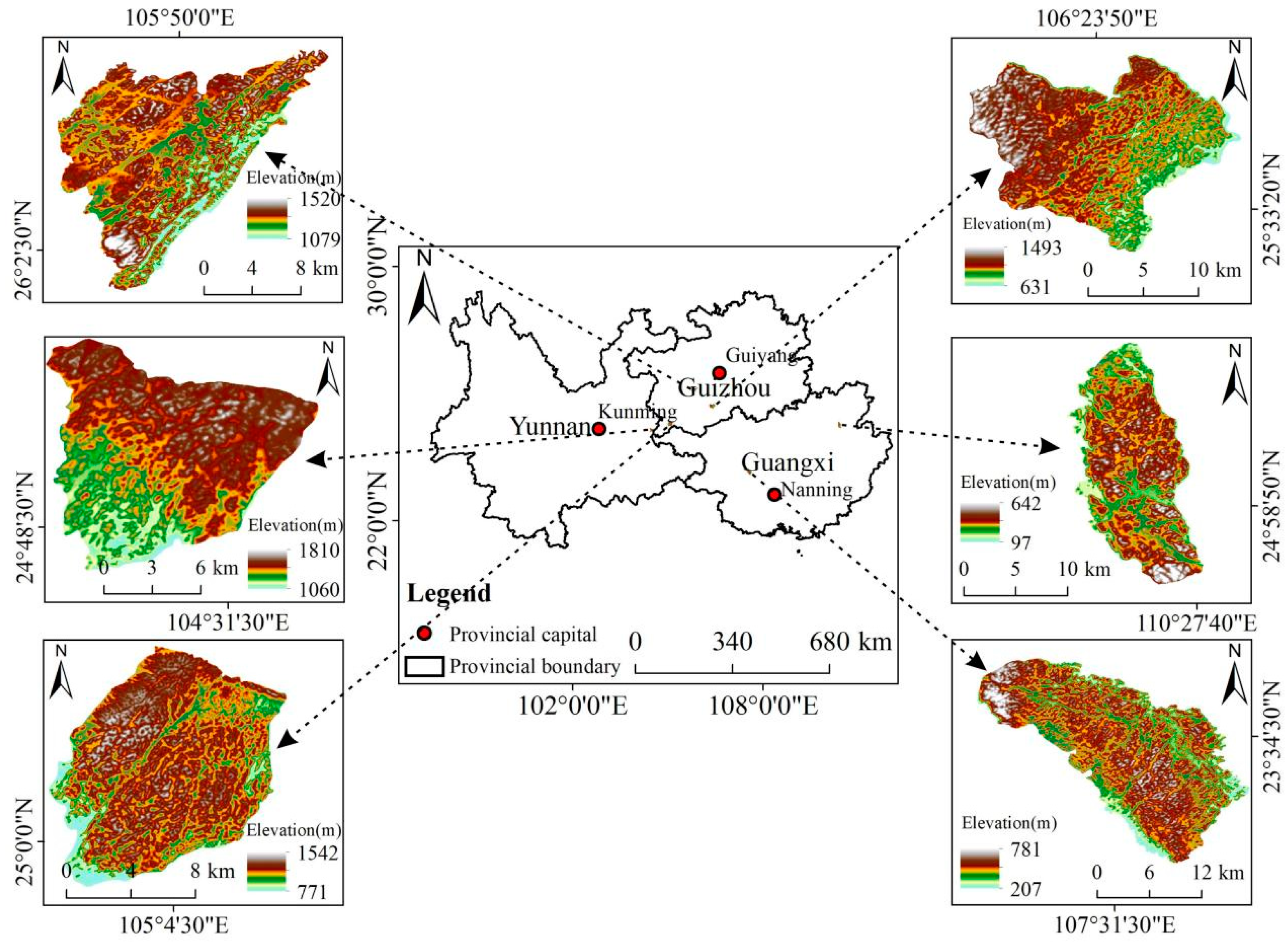
Figure 2.
Schematic diagram of the terrain opening algorithm. Modified from Yokohama et al. (2002).
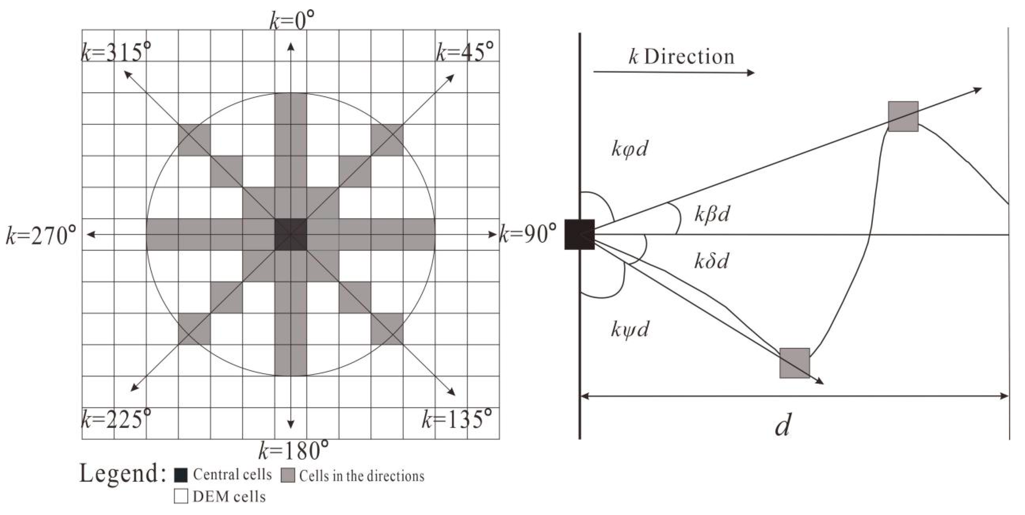
Figure 3.
Schematic of the (a) opening difference, (b) opening and closing operation binary diagram, and (c) positive and negative terrain boundaries.
Figure 3.
Schematic of the (a) opening difference, (b) opening and closing operation binary diagram, and (c) positive and negative terrain boundaries.
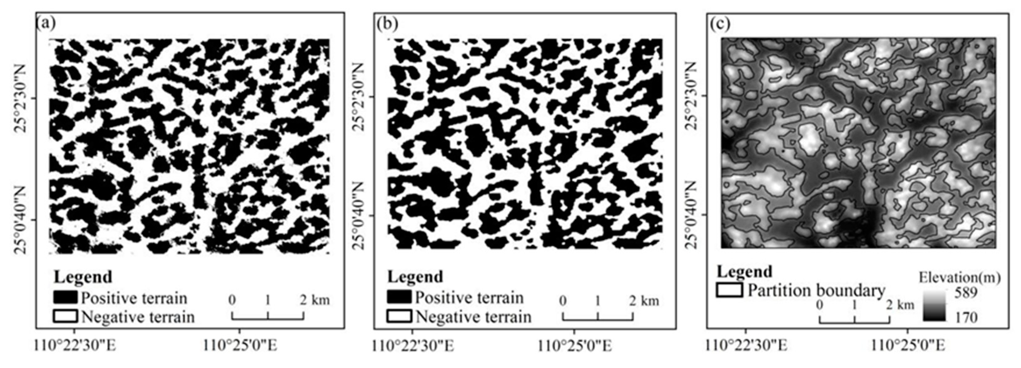
Figure 4.
(Left) View of the peaks and depressions in the karst area and (right) eight-direction slope changes.
Figure 4.
(Left) View of the peaks and depressions in the karst area and (right) eight-direction slope changes.
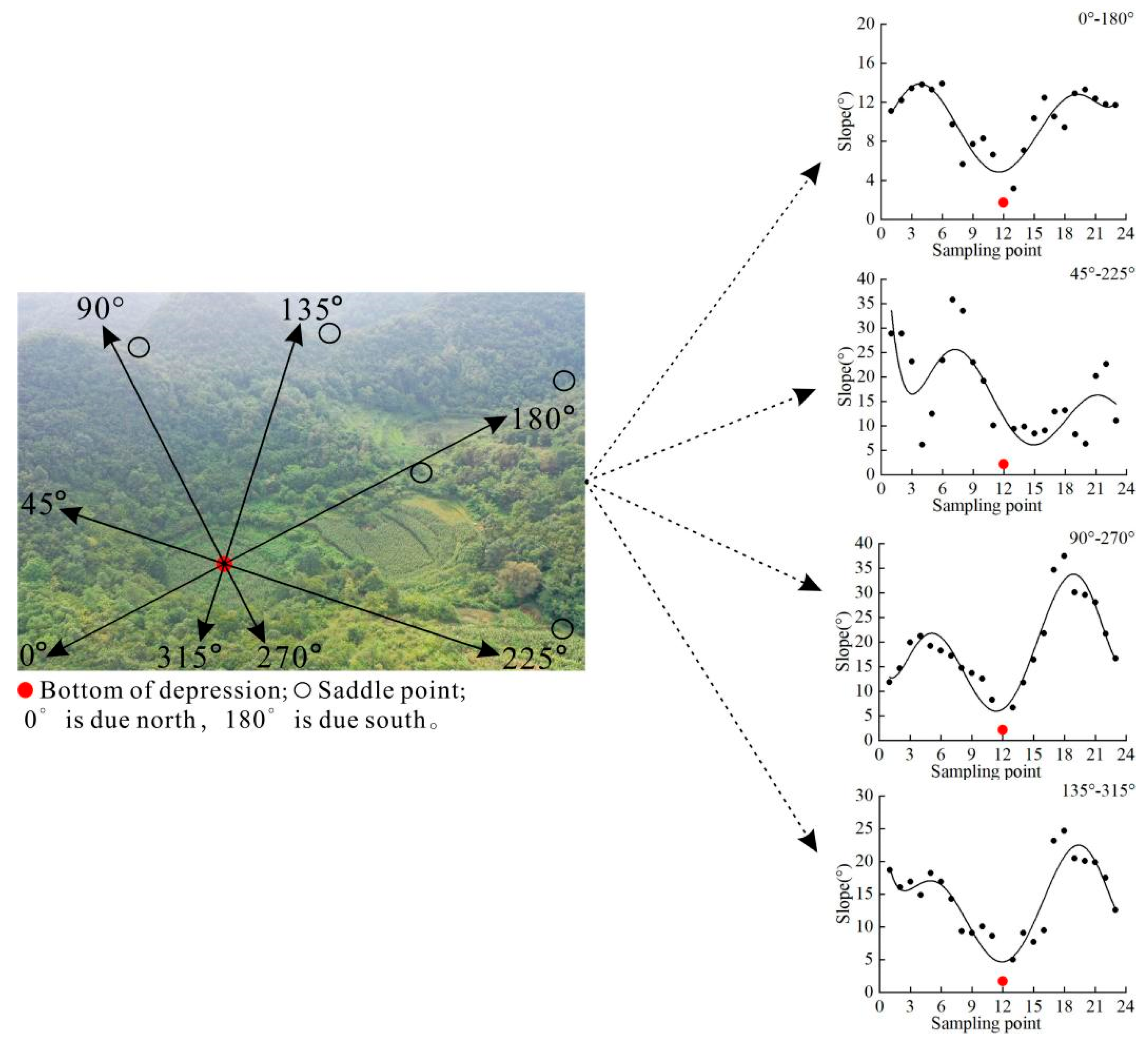
Figure 5.
Technical roadmap for detecting karst depressions using the ROBSMP.
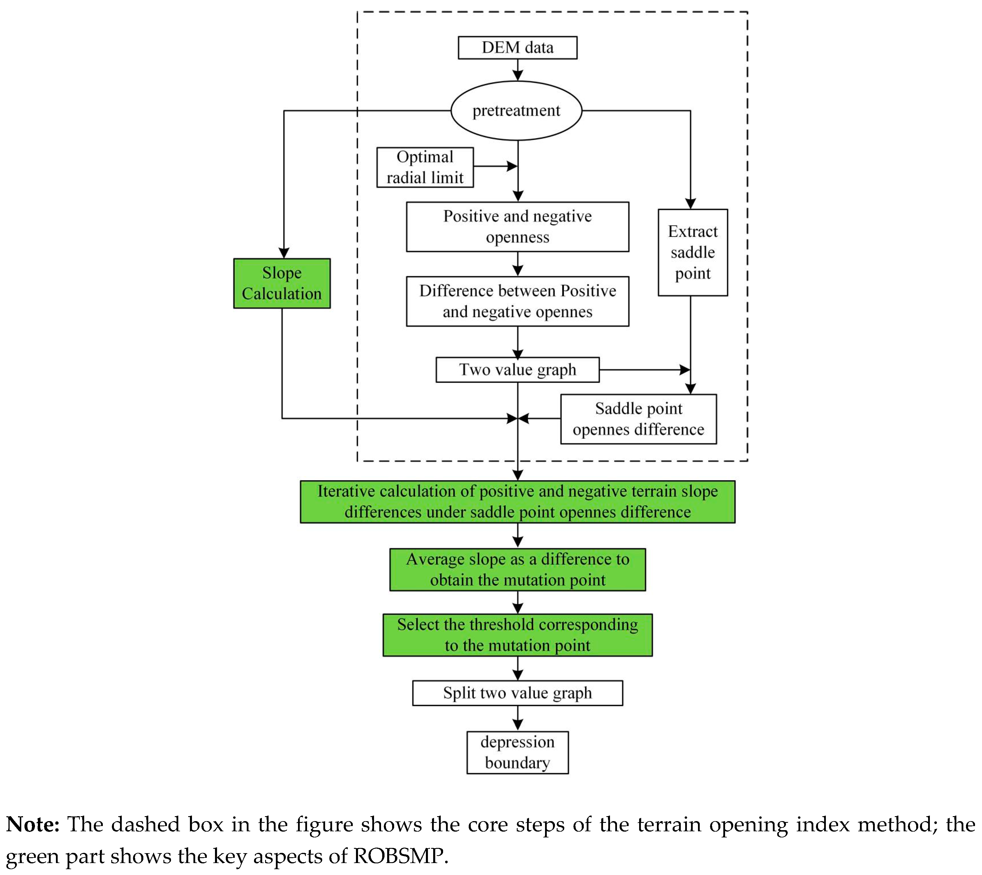
Figure 6.
Variation of the mean value of openness with the analysis radius in (a) Anshun, (b) Ziyun, (c) Xingyi, (d) Luoping, (e) Guilin, and (f) Pingguo sample areas.
Figure 6.
Variation of the mean value of openness with the analysis radius in (a) Anshun, (b) Ziyun, (c) Xingyi, (d) Luoping, (e) Guilin, and (f) Pingguo sample areas.
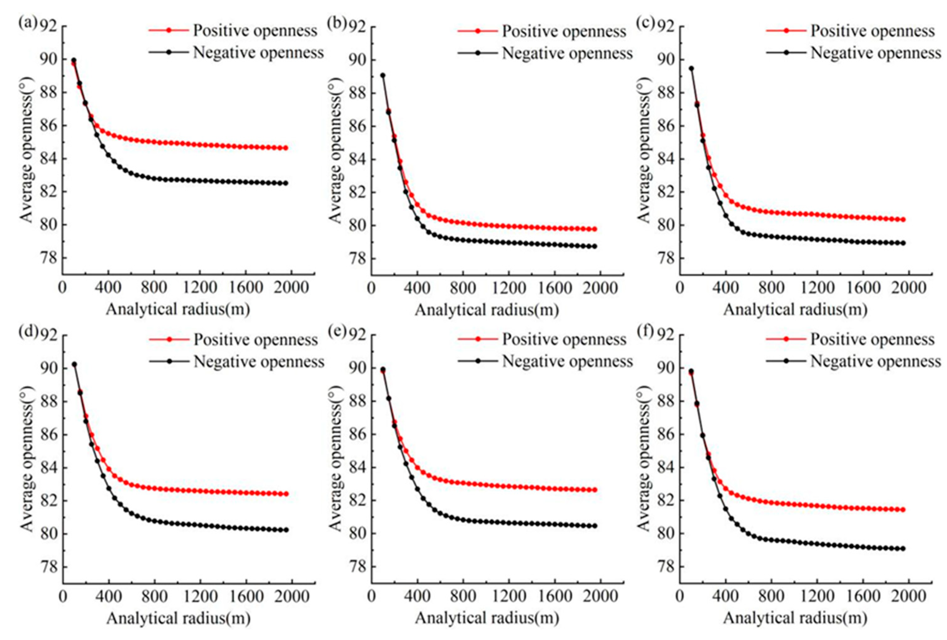
Figure 7.
Obtaining the optimal analysis radius of Anshun sample area (a), Ziyun sample area (b), Xingyi sample area (c), Luoping sample area (d), Guilin sample area (e), Pingguo sample area (f) by using mean-variable-point method.
Figure 7.
Obtaining the optimal analysis radius of Anshun sample area (a), Ziyun sample area (b), Xingyi sample area (c), Luoping sample area (d), Guilin sample area (e), Pingguo sample area (f) by using mean-variable-point method.
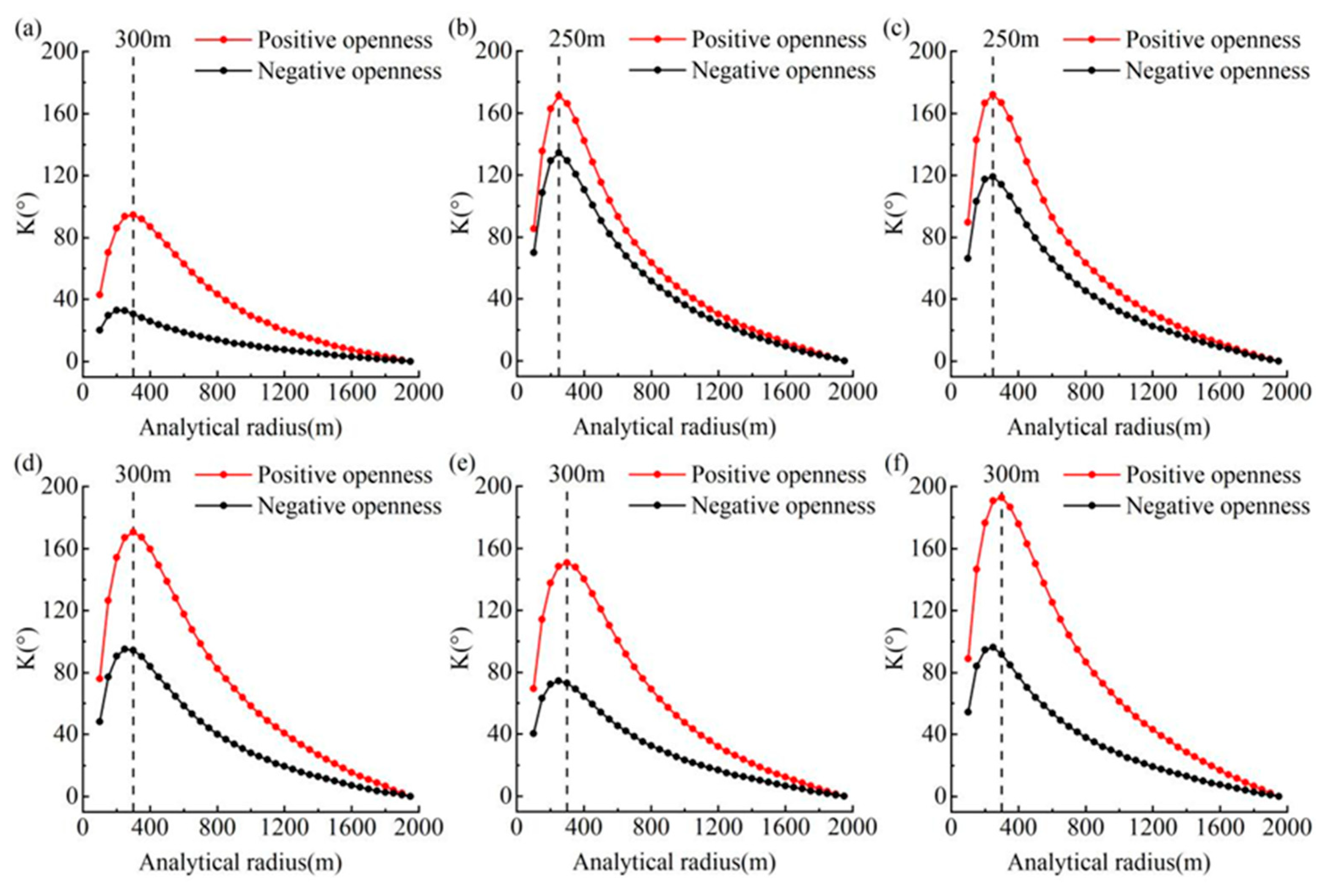
Figure 8.
Schematic diagram of saddle point distribution.
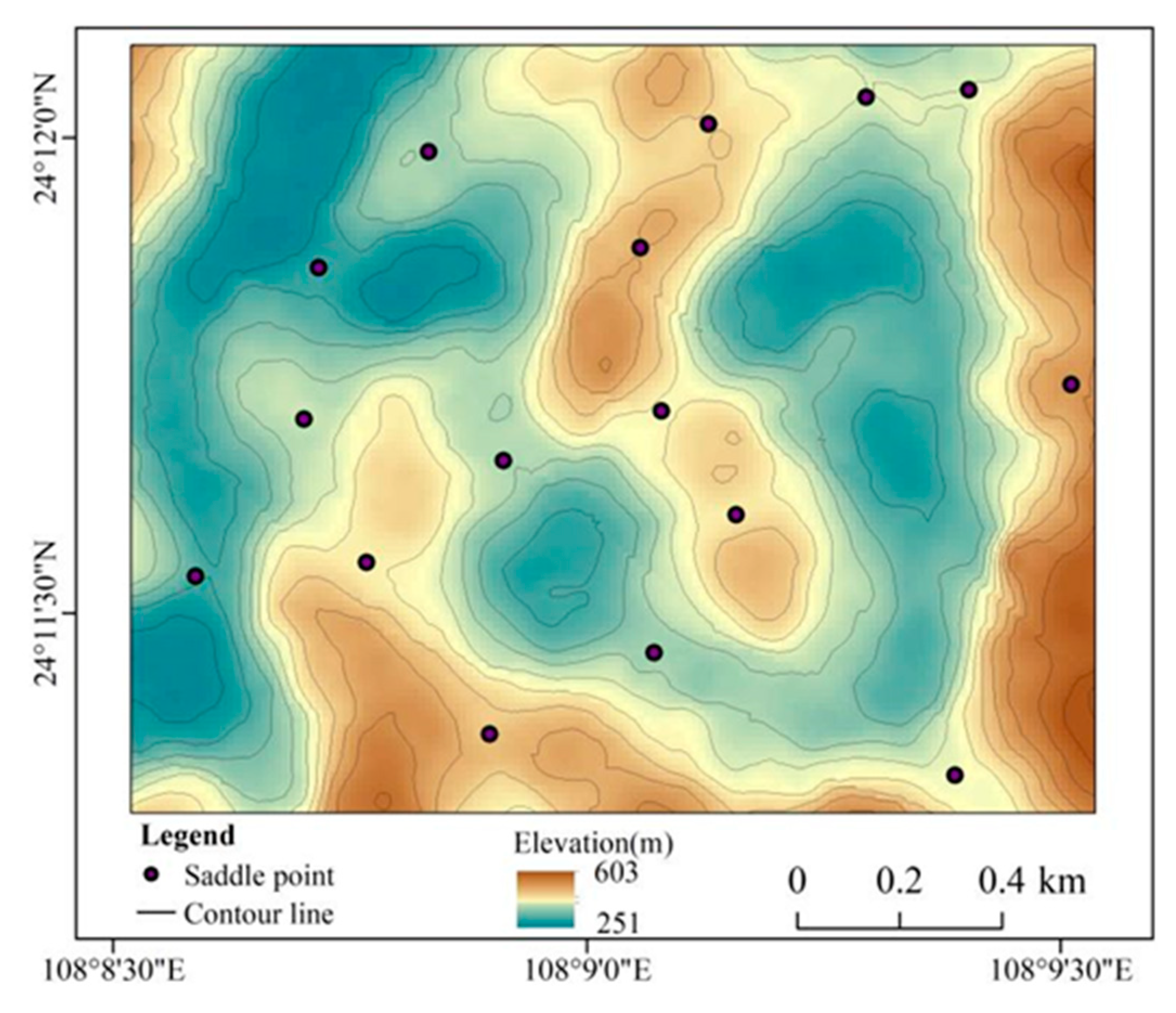
Figure 9.
Distribution statistics of topographic opening difference at saddle point.
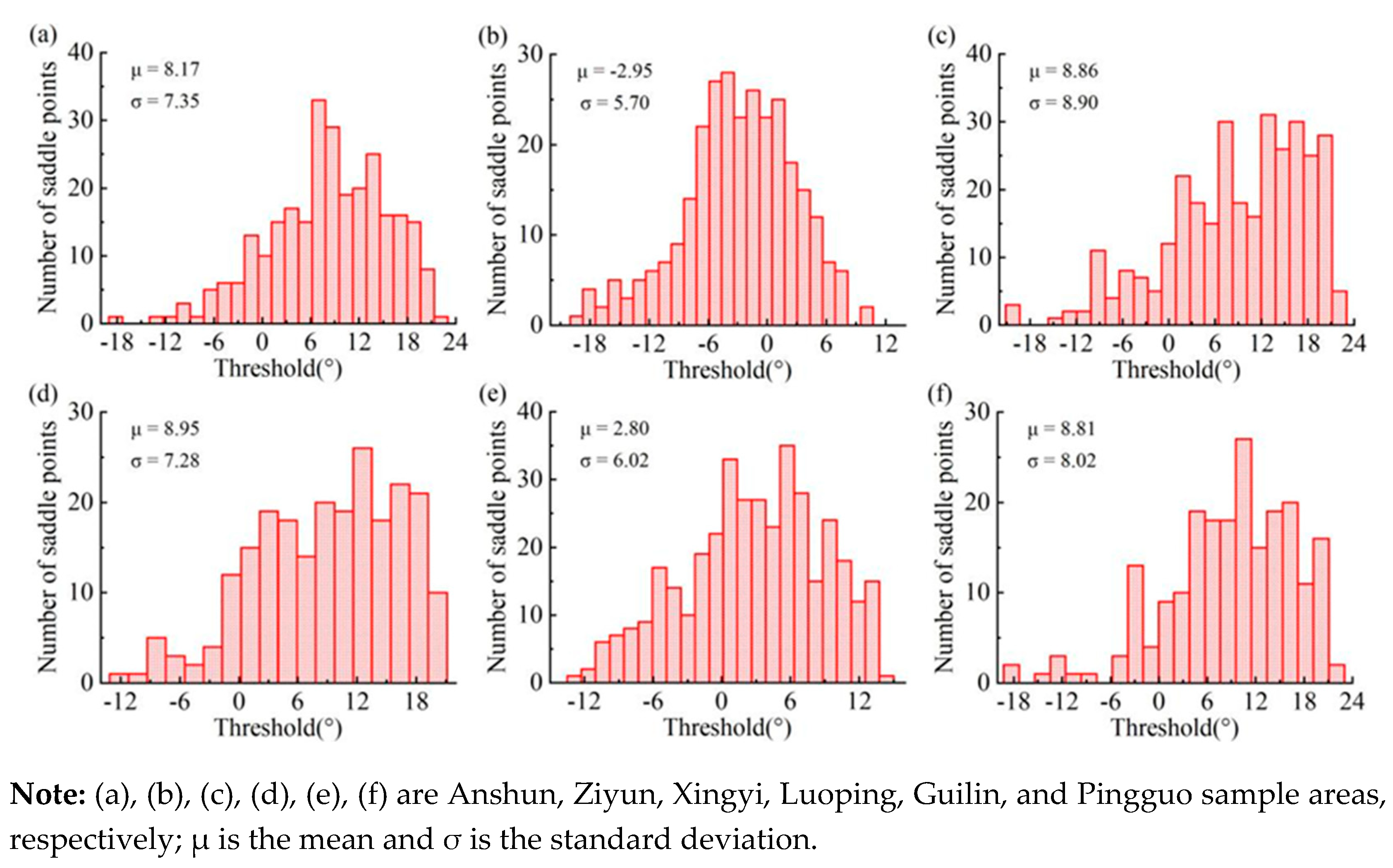
Figure 10.
Relationship between segmentation threshold and average slope difference in Anshun sample area (a), Ziyun sample area (b), Xingyi sample area (c), Luoping sample area (d), Guilin sample area (e), Pingguo sample area (f).
Figure 10.
Relationship between segmentation threshold and average slope difference in Anshun sample area (a), Ziyun sample area (b), Xingyi sample area (c), Luoping sample area (d), Guilin sample area (e), Pingguo sample area (f).
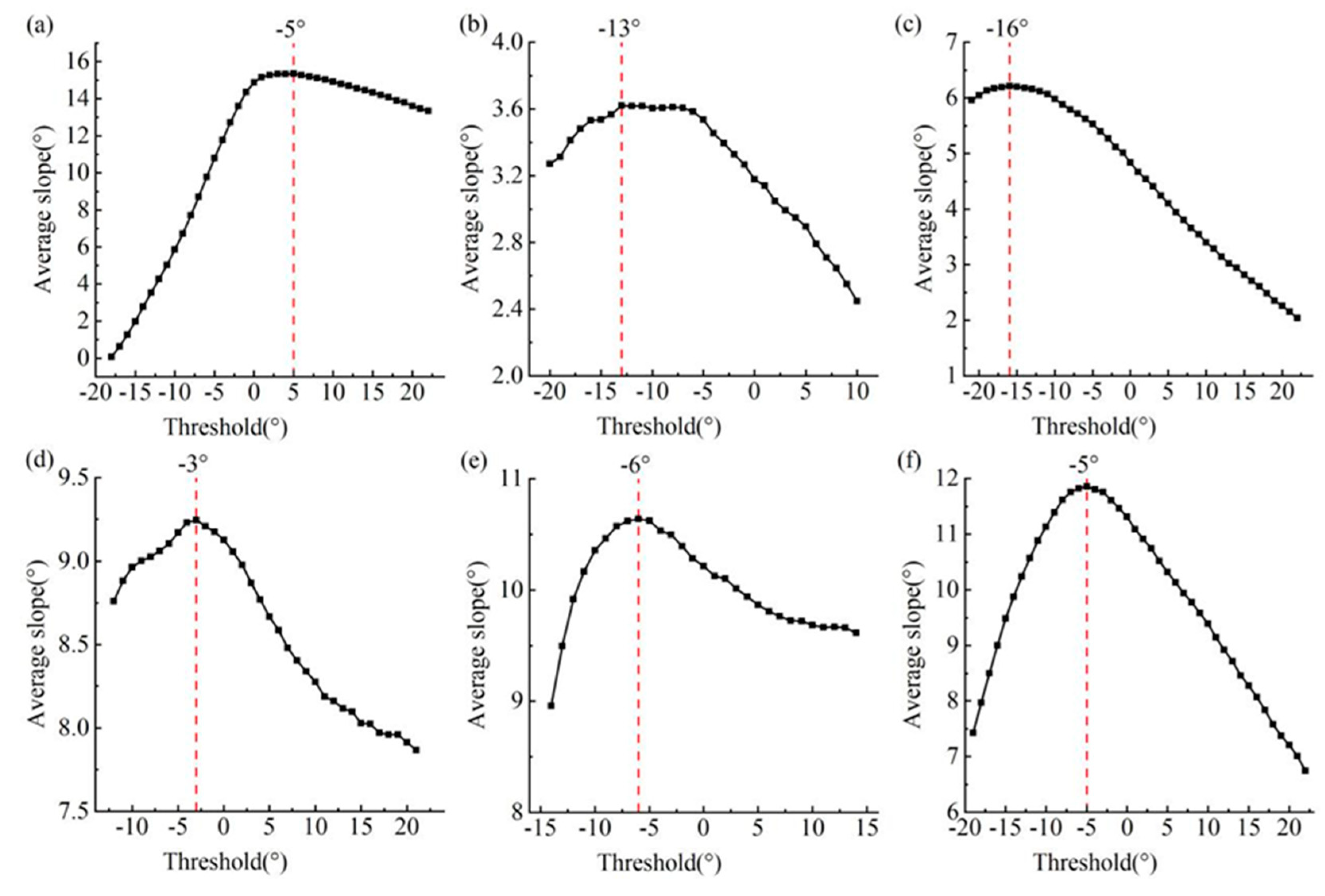
Figure 11.
(a), (b), (c), (d), (e), (f) Relationships between segmentation thresholds and mean slope difference in Anshun, Ziyun, Xingyi, Luoping, Guilin, and Pingguo sample areas, respectively.
Figure 11.
(a), (b), (c), (d), (e), (f) Relationships between segmentation thresholds and mean slope difference in Anshun, Ziyun, Xingyi, Luoping, Guilin, and Pingguo sample areas, respectively.
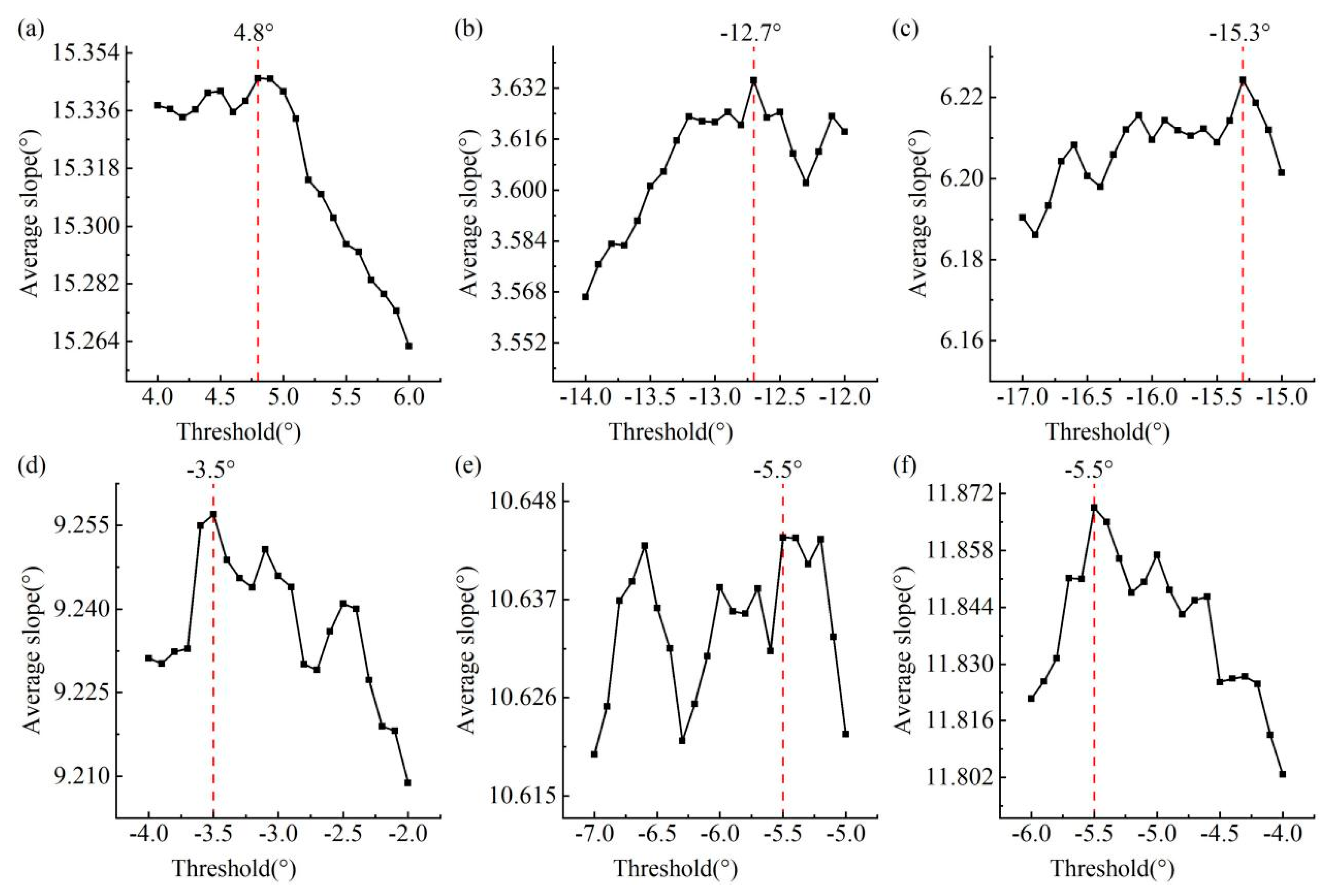
Figure 12.
Comparison of hand-drawn depression boundary lines with those extracted by terrain opening index method and ROBSMP.
Figure 12.
Comparison of hand-drawn depression boundary lines with those extracted by terrain opening index method and ROBSMP.
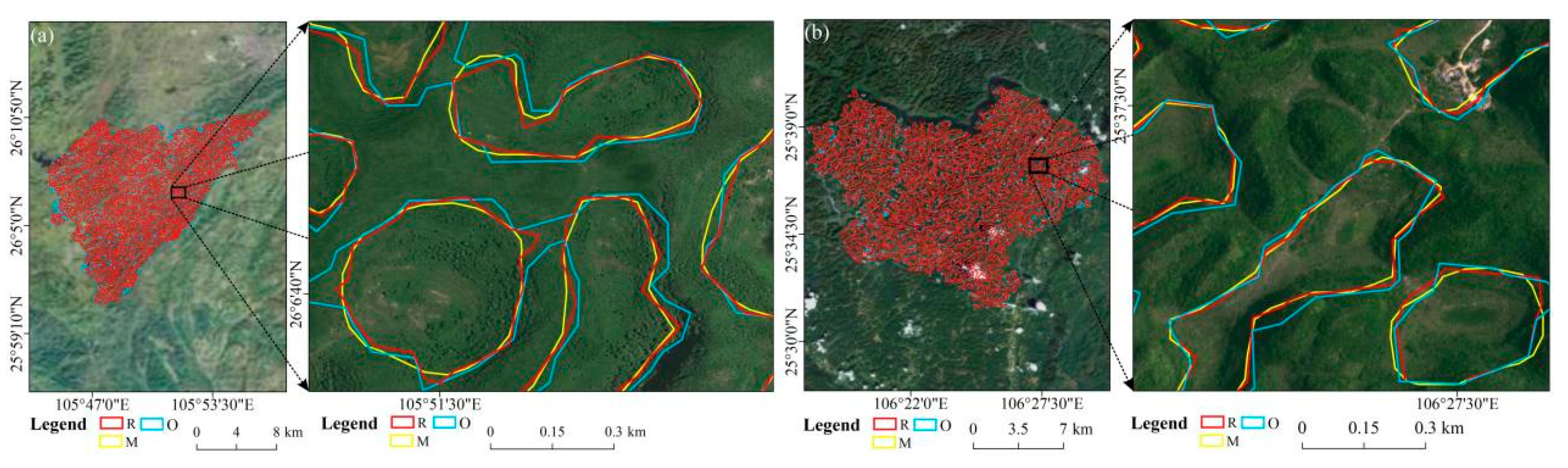
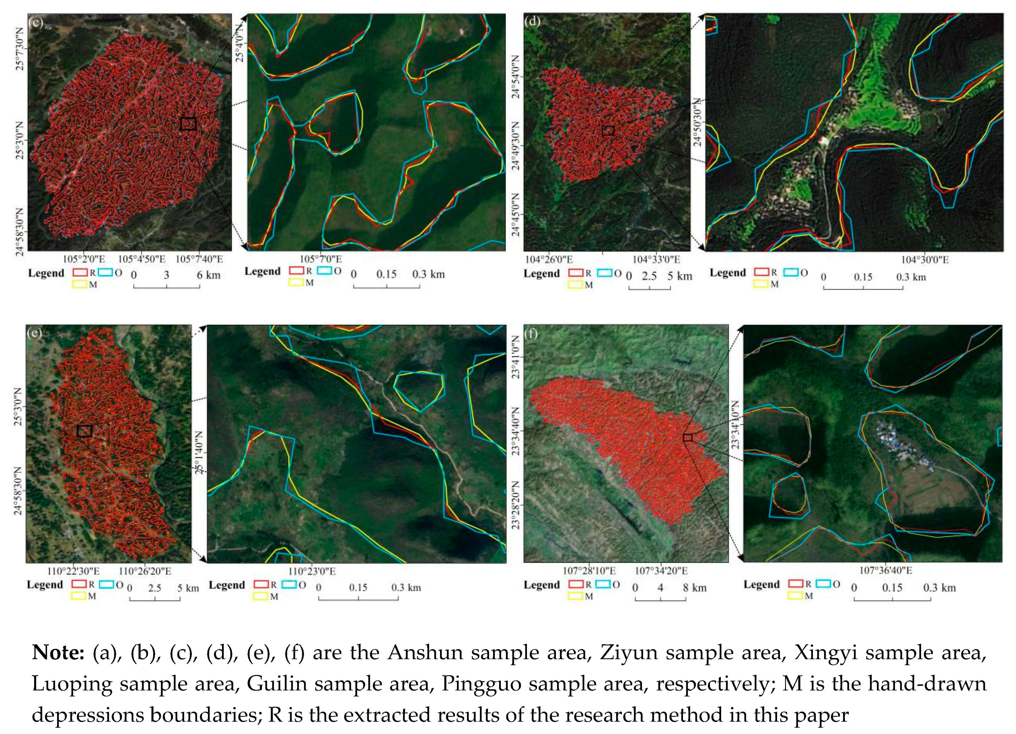
Figure 13.
Comparison of the effectiveness of the terrain opening index method and ROBSMP for extracting karst depressions.
Figure 13.
Comparison of the effectiveness of the terrain opening index method and ROBSMP for extracting karst depressions.
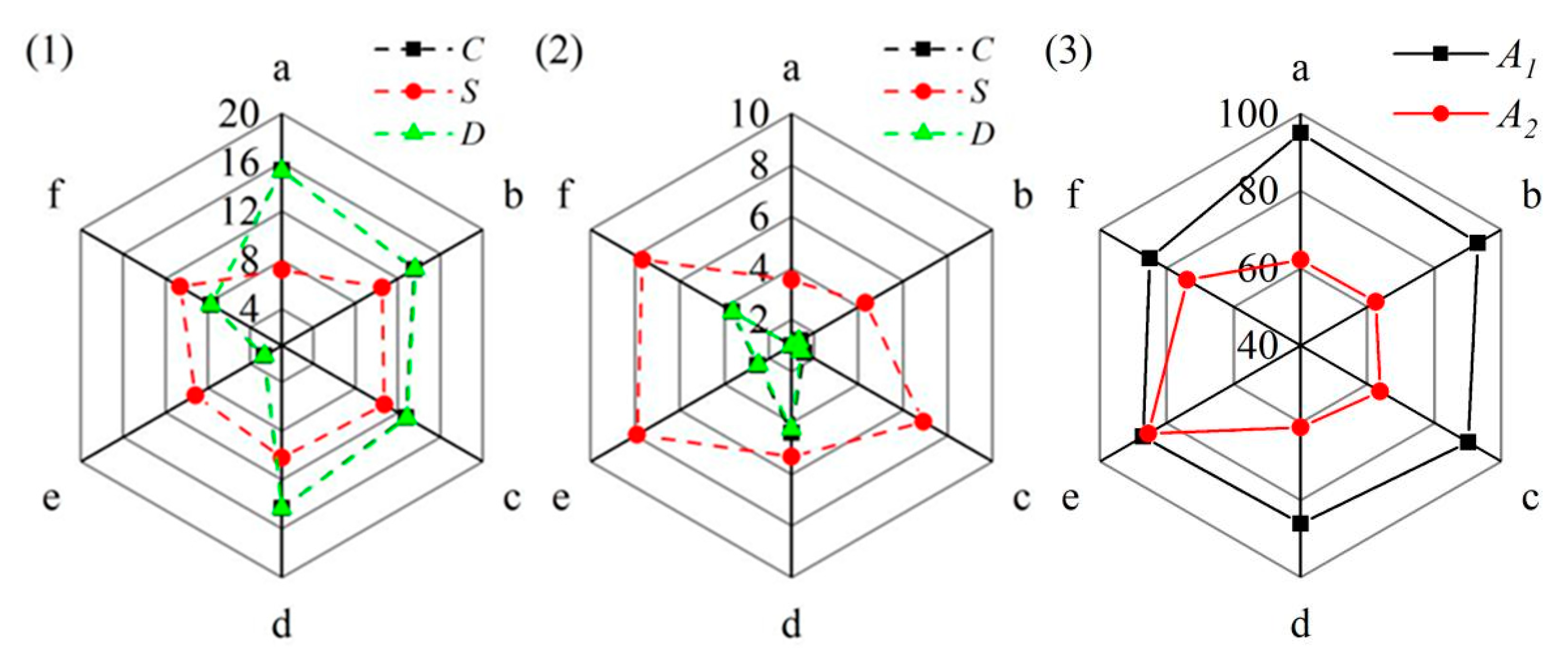
Figure 14.
Variation of the slope with the threshold value in the Qibaigang sample area.
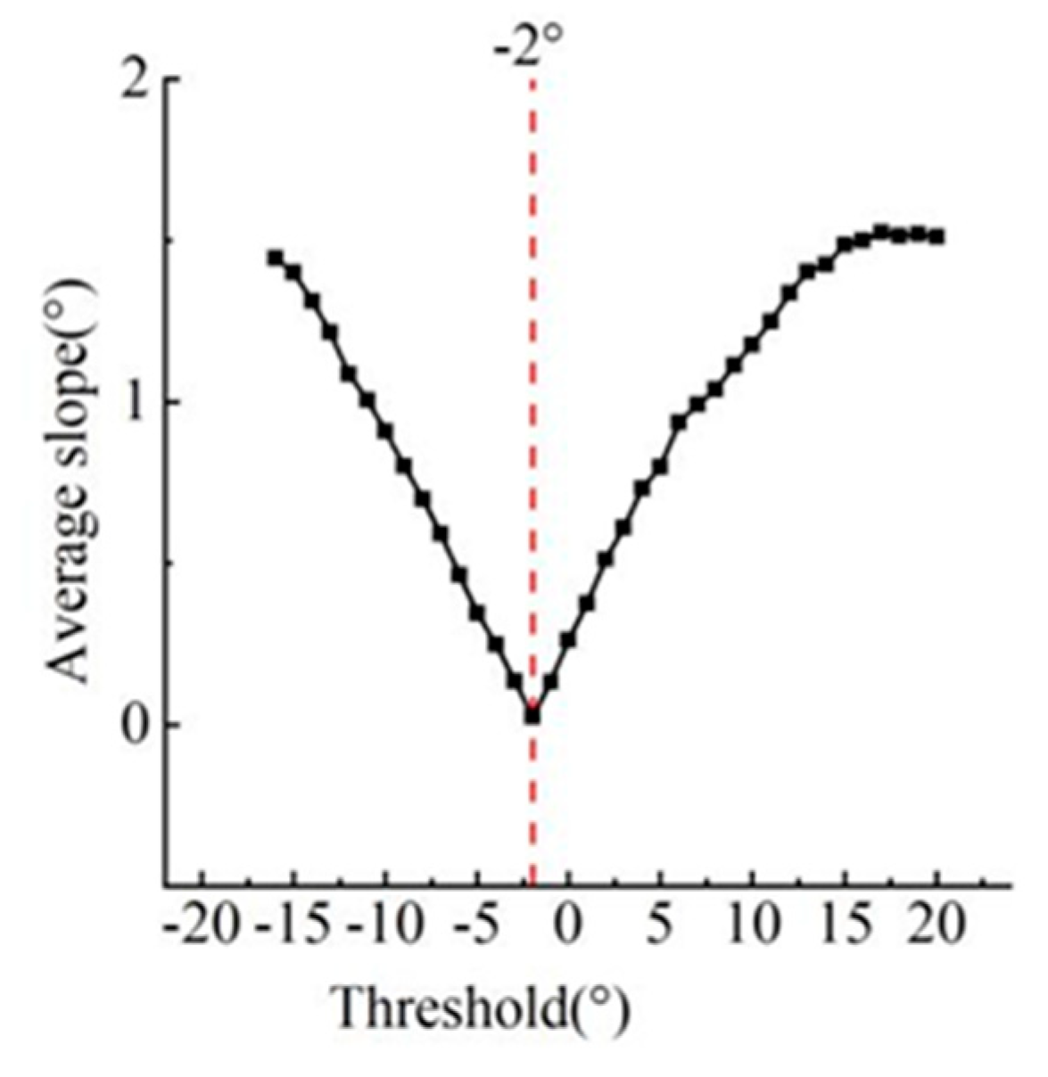
Figure 15.
Three-dimensional schematic of different types of depressions.
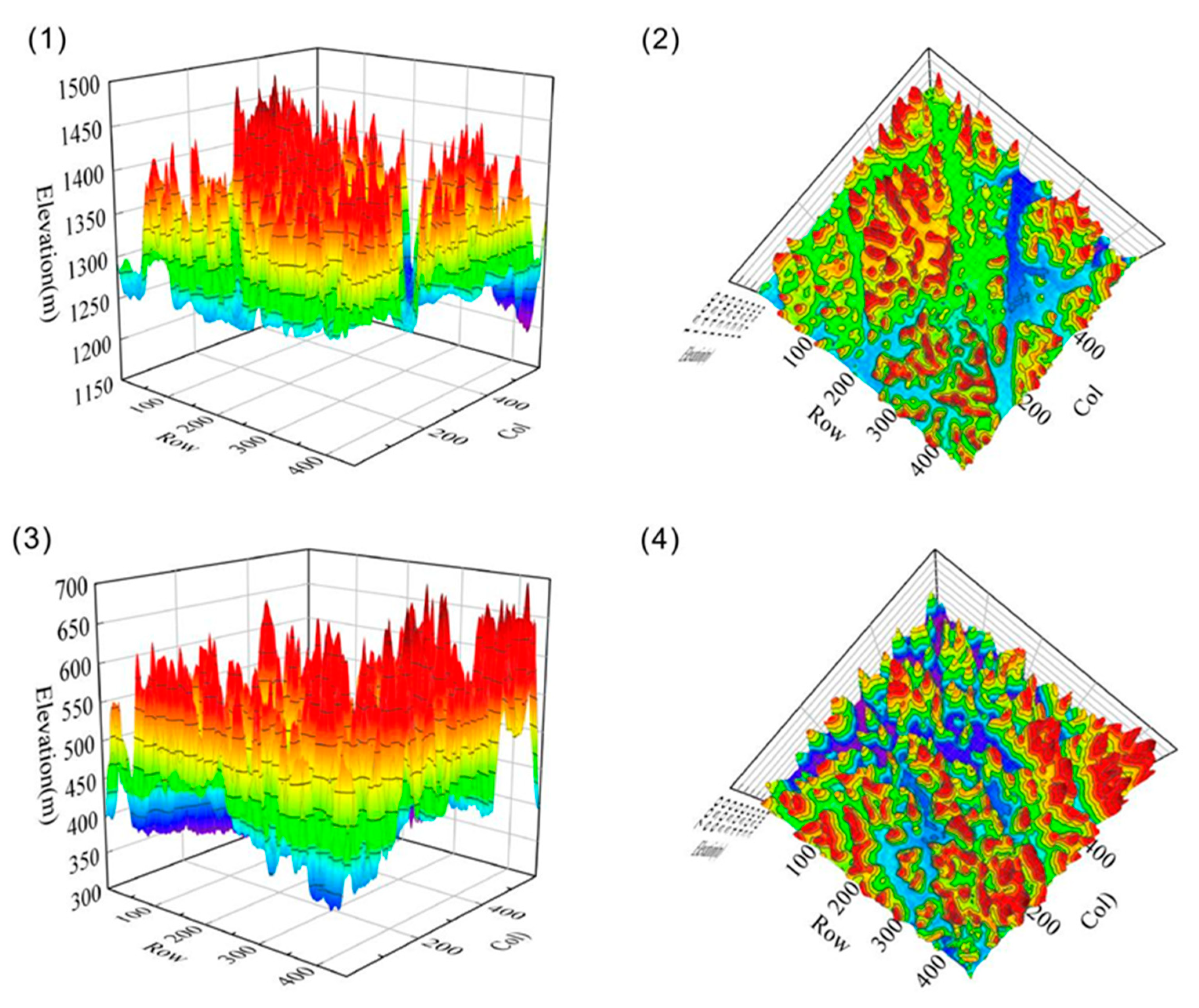
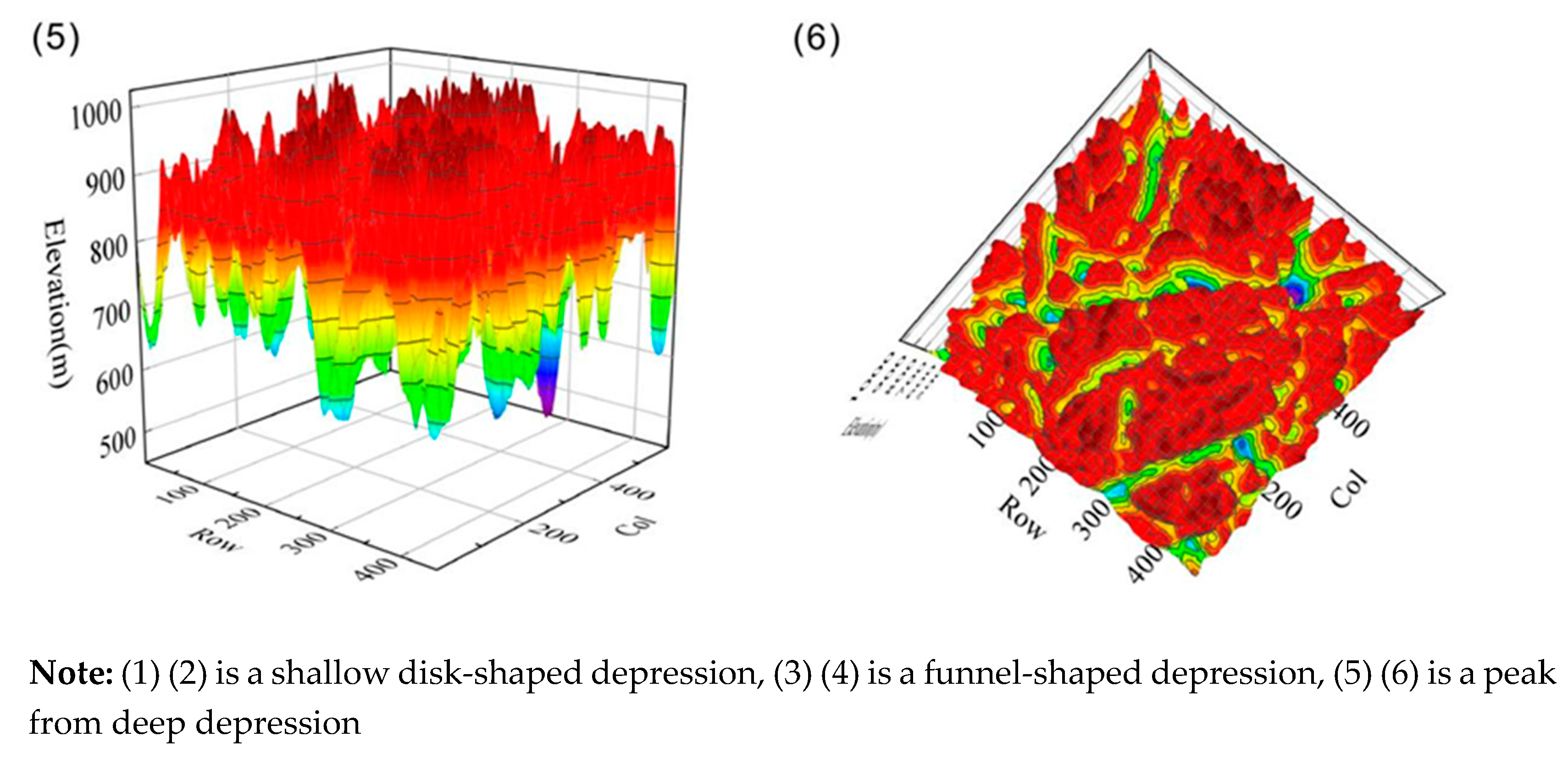

Table 1.
Basic overview of the study areas.
| Name of the study area | Longitude | Latitude | Area (km2) | Depression morphology | Administrative location |
| Anshun sample area | 105°44′34.29″–105°56′37.47″E | 26°0′41.80″–26°11′25.72″N | 191.36 | Shallow dish | Anshun City, Guizhou Province |
| Ziyun sample area | 106°17′35.13″–106°30′54.72″E | 25°31′14.83″–25°40′53.62″N | 223.45 | Funnel-type | Ziyun County, Guizhou Province |
| Xingyi sample area | 104°59′8.86″–105°9′20.75″E | 24°58′3.79″–25°8′23.07″N | 212.41 | Funnel-type | Xingyi City, Guizhou Province |
| Luoping sample area | 104°25′23.89″–104°34′31.81″E | 24°47′2.67″–24°54′48.99″N | 134.54 | Shallow dish | Luoping County, Yunnan Province |
| Guilin sample area | 110°20′50.10″–110°27′59.84″E | 24°54′44.49″–25°7′19.71″N | 163.91 | Funnel-type | Guilin City, Guangxi Zhuang Autonomous Region |
| Pingguo sample area | 107°22′58.08″–107°39′52.78″E | 23°26′48.56″–23°39′21.47″N | 317.92 | Funnel-type | Pingguo County, Guangxi Zhuang Autonomous Region |
Disclaimer/Publisher’s Note: The statements, opinions and data contained in all publications are solely those of the individual author(s) and contributor(s) and not of MDPI and/or the editor(s). MDPI and/or the editor(s) disclaim responsibility for any injury to people or property resulting from any ideas, methods, instructions or products referred to in the content. |
© 2024 by the authors. Licensee MDPI, Basel, Switzerland. This article is an open access article distributed under the terms and conditions of the Creative Commons Attribution (CC BY) license (http://creativecommons.org/licenses/by/4.0/).
Copyright: This open access article is published under a Creative Commons CC BY 4.0 license, which permit the free download, distribution, and reuse, provided that the author and preprint are cited in any reuse.


