
Submitted:
16 April 2024
Posted:
17 April 2024
You are already at the latest version
Abstract
The article presents an innovative method for synthesizing radiation patterns efficiently by 1
combining the Taguchi method and neural networks, while validating the results on a 10-element 2
antenna array. The Taguchi method aims to minimize product and process variability, while neural 3
networks are used to model the relationship between antenna design parameters and radiation 4
pattern characteristics. This approach utilizes Taguchi parameters as inputs for the neural network, 5
which is then trained on a dataset generated by the Taguchi method. After training, the network is 6
validated using a real 10-element antenna array. Analytical results demonstrate that this method 7
enables efficient synthesis of radiation patterns with a significant reduction in computation time 8
compared to traditional approaches. Furthermore, validation on the antenna array confirms the 9
accuracy and robustness of the approach, showing a high correlation between predicted performances 10
by the neural network model and actual measurements on the antenna array.In summary, our article 11
highlights that the combined use of the Taguchi method and neural networks, with validation on a 12
real antenna array, offers a promising approach for efficient synthesis of antenna radiation patterns. 13
This approach combines speed, accuracy, and reliability in antenna system design.
Keywords:
Taguchi
; Neural Networks
; Radiation pattern
; Phased antenna array
; Beamforming
1. Introduction
The synthesis of radiation patterns for antenna arrays stands as a pivotal discipline in both communication systems and radar system design. This sophisticated practice involves crafting and precisely controlling the radiation patterns of interconnected antennas to achieve specific performance goals in signal directionality and spatial coverage [1,2,3]. By amalgamating antenna theory with advanced signal processing techniques, this practice allows for the precise and adaptable shaping of antenna directional characteristics, offering remarkable flexibility in targeted signal transmission or reception. Sophisticated design methodologies are employed to optimize antenna configurations, yielding high efficiency in diverse applications such as high-performance wireless communication networks and advanced radar systems [4,5]. This introduction aims to explore the fundamental principles, design methodologies, and applications of this intricate yet indispensable discipline in the realm of antenna technologies [5,6]. In radar systems, these arrays revolutionize target detection and tracking by swiftly steering beams electronically, eliminating the need for cumbersome mechanical adjustments [7,8]. They form the backbone of modern communication networks, dynamically adapting to fluctuating environments by employing beamforming techniques to optimize signal strength and coverage. In space communications, their reliability becomes paramount, ensuring seamless connectivity between Earth and satellites, aiding in interplanetary exploration and satellite-based services [9]. Military and defense sectors harness their agility for surveillance, electronic warfare, and rapid response capabilities in ever-changing operational scenarios [10]. These arrays are catalysts for the evolution of wireless technologies, refining Wi-Fi, IoT connectivity, and upcoming standards like 5G, augmenting data rates, minimizing interference, and extending network reach [11]. Additionally, their role in medical imaging, especially in ultrasound systems, enables clinicians to achieve detailed, high-resolution images, revolutionizing diagnostic capabilities. These diverse and detailed applications underscore the pivotal role of phased antenna arrays across aviation, communication, defense, space exploration, healthcare, and wireless technologies [12,13]. Phased antenna arrays can be paired with neural networks for various applications. Integrating neural networks into phased arrays offers opportunities to optimize and dynamically adapt antenna operations based on environmental conditions and specific requirements. For instance, neural networks can predict and adjust optimal beam parameters in real time, enhancing signal quality and range in wireless communication networks. Similarly, in radar systems, neural networks can analyze radar return data sophisticatedly, aiding in more precise target detection, classification, and tracking by leveraging the learning capabilities of the neural network [14,15]. This fusion of phased antenna arrays with neural networks presents exciting prospects for intelligent adaptation and continual performance optimization across diverse fields like wireless communications, advanced radar surveillance, and other applications demanding heightened responsiveness and precision [16]. Phased antenna arrays play a pivotal role in the evolution of communication networks like 5G and the future advancements toward 6G. These antennas offer essential directionality and adaptability to meet the escalating demands for data throughput and connectivity in these next-generation communication networks [17,18,19,20]. With 5G, phased arrays are utilized for dynamic beamforming, enabling high-speed, low-latency communications, and improved coverage in dense environments [53]. Moving towards 6G [77], these antennas are poised to become even more critical, leveraging higher frequencies and emerging technologies to achieve faster speeds, ultra-low latency, and groundbreaking applications such as extended reality, holographic communications, and more. Phased antenna arrays will be instrumental in maximizing spectral and spatial efficiency, addressing the technological challenges inherent in these advancements in next-generation wireless networks [21,22,23].

2. Phased Antenna Arrays
Phased antenna arrays are intricate systems comprising multiple antenna elements, each capable of independent phase and amplitude adjustments in the signals they transmit or receive [28,29,30]. These adjustments enable the array to sculpt the radiation pattern of emitted waves or enhance reception sensitivity. By precisely coordinating these adjustments, the array achieves beamforming, directing a focused beam in specific directions without the need for physical repositioning. This capability proves invaluable in radar systems for swift target tracking and wide-area surveillance [31,32]. In communication networks, phased arrays facilitate adaptive beam steering, optimizing signal reception in dynamic and challenging environments. Despite the complexity inherent in managing numerous elements and ensuring their coordinated actions, ongoing advancements in technology continue to refine these arrays, making them more efficient, adaptable, and pivotal across diverse domains, including telecommunications, space exploration, and defense systems [33,34].
In the world of digital systems, the transition from conventional analog beamforming to digital processes involves intricate signal manipulation. This manipulation occurs at the baseband level, where precise adjustments are made to signal amplitude and phase digitally to align with the desired excitation pattern [35,36]. This departure from traditional analog beamforming involves specialized signal processing components.
Digital systems have the potential to generate a multitude of beams, designated as N, by merging signals from multiple sources [37]. The actual number of formed beams relies on the RF characteristics of M transmission channels and the computational capabilities of the signal processing modules [38].
Critical components such as digital-to-analog converters (DACs), analog-to-digital converters (ADCs), and signal processing modules play pivotal roles in this process. These components require exceptional speed, surpassing their analog counterparts, to efficiently process digital data and precisely shape analog signals [39]. This rapid processing capability serves as the bedrock of digital beamforming systems, enabling efficient signal manipulation within the digital realm—an essential aspect of their operational efficiency [40].
In fully digital beamforming systems, there’s a direct relationship between the number of amplifiers (such as Power Amplifiers - PAs and Low-Noise Amplifiers - LNAs) and the transmission channels. This connection categorizes these systems as active antenna array architectures [41,42]. Notably, these arrays possess reconfigurable properties, allowing for dynamic modifications in beam formations. This adaptability in altering beams designates these active antenna arrays as reconfigurable antenna arrays, providing flexibility and adaptiveness across diverse communication scenarios [43,44].
In this study, the optimization methodology we introduce was implemented using MATLAB scripts, providing a flexible and powerful platform for algorithm development and execution. Moreover, to enhance the user experience and facilitate a deeper understanding of the optimization process, we leveraged MATLAB’s Integrated Development Environment (IDE) to provide real-time visual feedback on the convergence of the optimization [45,46]. This interactive feature not only allowed for monitoring the optimization progress but also enabled researchers to make informed decisions regarding parameter adjustments or algorithm modifications during runtime. Such detailed insights into the optimization convergence serve to enrich the methodology and improve its effectiveness in practical applications [47,48,49].
Consider an antenna array consisting of N identical radiating elements. Each element of order n has its own radiation characteristic function and is fed by the current .
The electric field produced by the element of the antenna array at a point P, located in its far radiation zone, is then written:
with , is a unit vector in the direction of the field produced by the element. is the observation angle in the local coordinate system of the element.
is the position vector of the far point P in the local coordinate system of the element.
The total electric field radiated by the antenna array is the sum of all elementary field , , ..., . Consequently, the directions of observation are equal, the distances are considered equal to the distance r between the origin of the global coordinate system and the observation point P. In terms of phase, the difference in path between and r rewarded by as shown in Figure 1.
The resulting field is expressed as:
Replacing with its expression 1, the expression of becomes:
Or et pour .
Moreover, the relation between the position vectors is : therefore:
The total radiated field will be :
We consider the field radiated by the element at the origin of the global coordinate system. The equation of the total field becomes:
We assume to be the sum of the excitation phase of the element and the decompensation phase of the path difference for :
So the total field is written:
The equation 6 can be generalized as follows :
With is the vector of the electric field for K directions of radiation, is the vector of elementary antenna excitation’s, and X is the geometry matrix of the antenna array.
With is the vector of the electric field for K directions of radiation, is the vector of elementary antenna excitation’s, and X is the geometry matrix of the antenna array [49].
2.1. Structure of Antenna Arrays
A linear antenna array (Figure 2) has N radiating elements arranged on a line segment with an inter-element distance d which is not necessarily constant.
These elements are excited by a current of amplitude and phase .
The array factor, at a point very far found in the radiation area, is written as follows:
with represents the excitation phases of the element (the first antenna is chosen as the phase reference: ), represents the position of the element, is the wave number, is the angle of incidence of the desired signal, and is the wavelength of the signal.
3. Taguchi Method
The Taguchi method, pioneered by Genichi Taguchi, is a statistical approach used to enhance quality and optimize processes in engineering and manufacturing. When applied to antenna arrays, this method involves systematically adjusting various design parameters to improve the array’s performance [49,50].
In the realm of antenna arrays, employing the Taguchi method entails structured experimentation to refine factors influencing performance. These factors encompass elements like spacing, geometry, materials, feeding techniques, and other design attributes. Engineers conduct experiments based on this approach, aiming to identify the ideal combination of parameters that enhance metrics such as gain, directivity, radiation pattern, and sidelobe suppression [51,52].
Utilizing predefined experimental designs, known as orthogonal arrays, the Taguchi method efficiently explores numerous parameter combinations through a limited set of experiments. Statistical analysis of these outcomes aids in pinpointing the most influential parameters and determining the optimal settings for superior antenna performance [53].
By leveraging the Taguchi method in antenna array design, the goal is to elevate overall performance, reliability, and efficiency by systematically optimizing parameters using a statistically-driven approach [46,54]. In their quest to improve a satellite communication phased array antenna, engineers utilized the Taguchi method to optimize its design parameters. They systematically experimented with element spacing, feeding techniques, and substrate materials, varying them across different levels. Analyzing resulting data on gain, beamwidth, and sidelobe levels using statistical methods, they pinpointed the most impactful factors and identified the ideal combination of element spacing, feeding technique, and substrate material. This optimized configuration maximized gain, narrowed beamwidth, and minimized side lobes, significantly enhancing the antenna’s performance in satellite communication [55,56].
3.1. Amplitude Synthesis of Antenna Array Radiation Pattern under Constraints
In this type of synthesis, constraints are imposed on the levels of sidelobes and the locations of nulls in the radiation pattern, which the beam towards interfering signals should exhibit. In this initial synthesis type, the Taguchi optimization procedure will be applied to three linear antenna arrays, each with a different number of sources (10, 16, and 24), in order to minimize sidelobes [46,49].
3.1.1. 10-Element Antenna Array
The array factor is described by the following equation.
To minimize sidelobe levels, the fitness function is chosen based on the optimization objective.
subject to constraints
To simplify the task and enhance understanding of this application, let’s elaborate on the Taguchi optimization procedure:
First Step: Initialization Problem
The first step involves selecting an appropriate experimental design and a well-structured fitness function. There are 5 parameters that need optimization. Therefore, the chosen orthogonal experimental design should have 5 columns () to represent these parameters. To capture nonlinear effects, three levels () for each parameter are deemed sufficient. Typically, an orthogonal experimental design with a strength of 2 () is effective for most problems. In summary, an orthogonal experimental design with 5 columns, 3 levels, and a strength of 2 is required.
Second Step: Designating Input Parameters
After accessing the online database OA , an orthogonal array (OA) (27, 5, 3, 2) is available, as indicated in Table 2. The fitness function is chosen based on the optimization objective. In this optimization example, the function is selected to achieve a low sidelobe level. The input parameters need to be selected for conducting experiments. When the orthogonal experimental design is chosen, numerical values corresponding to the three levels of each input parameter must be determined in the first iteration. The value for level 2 is selected at the midpoint of the optimization range. The values for levels 1 and 3 are calculated using the following equations.
Numerical Application:
Table 2.
Taguchi Experimental Design (N=27, K=5, S=3, t=2)
| Experiment | |||||
|---|---|---|---|---|---|
| 1 | 1 | 1 | 1 | 1 | 1 |
| 2 | 2 | 1 | 2 | 2 | 2 |
| 3 | 3 | 1 | 3 | 3 | 3 |
| 4 | 1 | 2 | 1 | 2 | 2 |
| 5 | 2 | 2 | 2 | 3 | 3 |
| 6 | 3 | 2 | 3 | 1 | 1 |
| 7 | 1 | 3 | 1 | 3 | 3 |
| 8 | 2 | 3 | 2 | 1 | 1 |
| 9 | 3 | 3 | 3 | 2 | 2 |
| 10 | 1 | 1 | 2 | 1 | 2 |
| 11 | 2 | 1 | 3 | 2 | 3 |
| 12 | 3 | 1 | 1 | 3 | 1 |
| 13 | 1 | 2 | 2 | 2 | 3 |
| 14 | 2 | 2 | 3 | 3 | 1 |
| 15 | 3 | 2 | 1 | 1 | 2 |
| 16 | 1 | 3 | 2 | 3 | 1 |
| 17 | 2 | 3 | 3 | 1 | 2 |
| 18 | 3 | 3 | 1 | 2 | 3 |
| 19 | 1 | 1 | 3 | 1 | 3 |
| 20 | 2 | 1 | 1 | 2 | 1 |
| 21 | 3 | 1 | 2 | 3 | 2 |
| 22 | 1 | 2 | 3 | 2 | 1 |
| 23 | 2 | 2 | 1 | 3 | 2 |
| 24 | 3 | 2 | 2 | 1 | 3 |
| 25 | 1 | 3 | 3 | 3 | 2 |
| 26 | 2 | 3 | 1 | 1 | 3 |
| 27 | 3 | 3 | 2 | 2 | 1 |
Using these equations, Table 2 can be converted into numerical values as shown in Table 3.
Table 3.
The numerical values of the levels in the first iteration.
| Experiment | |||||
|---|---|---|---|---|---|
| 1 | 0.25 | 0.25 | 0.25 | 0.25 | 0.25 |
| 2 | 0.5 | 0.25 | 0.5 | 0.5 | 0.5 |
| 3 | 0.75 | 0.25 | 0.75 | 0.75 | 0.75 |
| 4 | 0.25 | 0.5 | 0.25 | 0.5 | 0.5 |
| 5 | 0.5 | 0.5 | 0.5 | 0.75 | 0.75 |
| 6 | 0.75 | 0.5 | 0.75 | 0.25 | 0.25 |
| 7 | 0.25 | 0.75 | 0.25 | 0.75 | 0.75 |
| 8 | 0.5 | 0.75 | 0.5 | 0.25 | 0.25 |
| 9 | 0.75 | 0.75 | 0.75 | 0.5 | 0.5 |
| 10 | 0.25 | 0.25 | 0.5 | 0.25 | 0.5 |
| 11 | 0.5 | 0.25 | 0.75 | 0.5 | 0.75 |
| 12 | 0.75 | 0.25 | 0.25 | 0.75 | 0.25 |
| 13 | 0.25 | 0.5 | 0.5 | 0.5 | 0.75 |
| 14 | 0.5 | 0.5 | 0.75 | 0.75 | 0.25 |
| 15 | 0.75 | 0.5 | 0.25 | 0.25 | 0.5 |
| 16 | 0.25 | 0.75 | 0.5 | 0.75 | 0.25 |
| 17 | 0.5 | 0.75 | 0.75 | 0.25 | 0.5 |
| 18 | 0.75 | 0.75 | 0.25 | 0.5 | 0.75 |
| 19 | 0.25 | 0.25 | 0.75 | 0.25 | 0.75 |
| 20 | 0.5 | 0.25 | 0.25 | 0.5 | 0.25 |
| 21 | 0.75 | 0.25 | 0.5 | 0.75 | 0.5 |
| 22 | 0.25 | 0.5 | 0.75 | 0.5 | 0.25 |
| 23 | 0.5 | 0.5 | 0.25 | 0.75 | 0.5 |
| 24 | 0.75 | 0.5 | 0.5 | 0.25 | 0.75 |
| 25 | 0.25 | 0.75 | 0.75 | 0.75 | 0.5 |
| 26 | 0.5 | 0.75 | 0.25 | 0.25 | 0.75 |
| 27 | 0.75 | 0.75 | 0.5 | 0.5 | 0.25 |
Third Step: Conducting Experiments and Building a Response Table
After determining the input parameters, the fitness function for each experiment can be calculated. For instance, the fitness value for experiment 1 (i.e., the first row of Table 3) is computed using Equation (14), resulting in 12.97. Then, the fitness value in the Taguchi method is converted to signal-to-noise ratio (S/N), denoted as ( ), using formula (14). The corresponding fitness values and the S/N ratios are listed in Table 4. These results are then used to construct a Response Table 4 for the first iteration by averaging the ratios for each parameter." The corresponding signal-to-noise ratio values are listed in Table 5. These results are then used to construct a Response Table (Table 5) by averaging the signal-to-noise ratios ( ) for each parameter using the following equation (3.9)- [46,49].
- n: Number of parameters
- m: Number of levels (1, 2, 3)
- N: Number of level combinations
- i: i-th iteration
For example, the average of the ratios (S/N) for and is.
Table 4.
Experiments and Fitness Values.
| Experiment | Fitness R | (S/N) | |||||
|---|---|---|---|---|---|---|---|
| 1 | 0.25 | 0.25 | 0.25 | 0.25 | 0.25 | 12.97 | -22.26 |
| 2 | 0.5 | 0.25 | 0.5 | 0.5 | 0.5 | 11.19 | -20.98 |
| 3 | 0.75 | 0.25 | 0.75 | 0.75 | 0.75 | 10.56 | -20.47 |
| 4 | 0.25 | 0.5 | 0.25 | 0.5 | 0.5 | 9.91 | -19.92 |
| 5 | 0.5 | 0.5 | 0.5 | 0.75 | 0.75 | 9.70 | -19.73 |
| 6 | 0.75 | 0.5 | 0.75 | 0.25 | 0.25 | 13.86 | -22.83 |
| 7 | 0.25 | 0.75 | 0.25 | 0.75 | 0.75 | 8.67 | -18.76 |
| 8 | 0.5 | 0.75 | 0.5 | 0.25 | 0.25 | 15.53 | -23.82 |
| 9 | 0.75 | 0.75 | 0.75 | 0.5 | 0.5 | 16.81 | -24.51 |
| 10 | 0.25 | 0.25 | 0.5 | 0.25 | 0.5 | 9.32 | -19.39 |
| 11 | 0.5 | 0.25 | 0.75 | 0.5 | 0.75 | 9.31 | -19.38 |
| 12 | 0.75 | 0.25 | 0.25 | 0.75 | 0.25 | 7.61 | -17.63 |
| 13 | 0.25 | 0.5 | 0.5 | 0.5 | 0.75 | 8.28 | -18.36 |
| 14 | 0.5 | 0.5 | 0.75 | 0.75 | 0.25 | 9.88 | -19.90 |
| 15 | 0.75 | 0.5 | 0.25 | 0.25 | 0.5 | 10.99 | -20.82 |
| 16 | 0.25 | 0.75 | 0.5 | 0.75 | 0.25 | 9.03 | -19.12 |
| 17 | 0.5 | 0.75 | 0.75 | 0.25 | 0.5 | 13.93 | -22.88 |
| 18 | 0.75 | 0.75 | 0.25 | 0.5 | 0.75 | 11.27 | -21.04 |
| 19 | 0.25 | 0.25 | 0.75 | 0.25 | 0.75 | 6.84 | -16.70 |
| 20 | 0.5 | 0.25 | 0.25 | 0.5 | 0.25 | 10.13 | -20.11 |
| 21 | 0.75 | 0.25 | 0.5 | 0.75 | 0.5 | 9.70 | -19.73 |
| 22 | 0.25 | 0.5 | 0.75 | 0.5 | 0.25 | 8.26 | -18.34 |
| 23 | 0.5 | 0.5 | 0.25 | 0.75 | 0.5 | 10.97 | -20.81 |
| 24 | 0.75 | 0.5 | 0.5 | 0.25 | 0.75 | 10.95 | -20.78 |
| 25 | 0.25 | 0.75 | 0.75 | 0.75 | 0.5 | 8.28 | -18.36 |
| 26 | 0.5 | 0.75 | 0.25 | 0.25 | 0.75 | 7.90 | -17.96 |
| 27 | 0.75 | 0.75 | 0.5 | 0.5 | 0.25 | 21.51 | -26.65 |
To identify the optimal level value for each parameter, it is necessary to find the highest signal-to-noise (S/N) ratio within each column of Table 4. This is highlighted in Table 5. Once the optimal levels are identified, a confirmation test is conducted using the corresponding numerical values of these optimal levels in the response table, Table 6 [46,49,84].
Table 5.
Response table (in decibels) after the first iteration-Element Levels (dB).
| Elements | 1 | 2 | 3 | 4 | 5 |
|---|---|---|---|---|---|
| Level 1 | -19.02 | -19.63 | -19.92 | -20.83 | -21.18 |
| Level 2 | -20.62 | -20.17 | -20.95 | -21.03 | -20.82 |
| Level 3 | -21.61 | -21.46 | -20.38 | -19.39 | -19.24 |
If the results from the current iteration do not meet the termination criteria, which are examined using Equation (23), and after determining the optimal level values from the current iteration that are used as central values for the next iteration (24) in our case, the central values for the next iteration are ;;;;; the optimization process is repeated in the subsequent iteration, reducing the optimization interval using Equation (25).
In this optimization example, the reduced function () is set to .
Table 6.
Optimized values of and maximum SLL for networks
| Optimized values of | Maximum SLL |
|---|---|
| 1.0000 | -13.1526 |
| 0.8413 | -22.8982 |
| 0.9322 | |
| 0.7675 | |
| 0.6049 | |
| 0.5715 | |
| 0.4746 | |
| 0.4877 |
This first type of synthesis (amplitude synthesis under constraint) aims to minimize the secondary lobes as much as possible, using our optimization technique. In Figure 3(a), the obtained results demonstrate successful minimization of the secondary lobe level (SLL or Side-Lobe-Level) down to dB, where the gain is approximately dB higher compared to the secondary lobe level of the uniform linear antenna array (SLL = dB). The optimization objective is achieved after 80 iterations as indicated in Figure 3(b). The excitation weights of this antenna array optimized by the Taguchi method are mentioned in Table 7.
Table 7.
Table of elements and weights.
| Elements | 1 | 2 | 3 | 4 | 5 |
|---|---|---|---|---|---|
| Weights | 1.0000 | 0.8984 | 0.7187 | 0.5015 | 0.3857 |
By comparing the results obtained with those of PSO (Particle Swarm Optimization) (see Figure 4), we observe:
- A gain of 0.6 dB in terms of secondary lobes minimization.
- A convergence speed of 80 iterations for the Taguchi method.
- The real-time required for our digital optimization tool is approximately 10 seconds.
With this method, we aim to minimize the error criterion; this amounts to minimizing the difference between the desired pattern (template) and the pattern obtained through synthesis.
3.1.2. 16-Element Antenna Array
In this example, the array factor is described by the following Equation (26).
The fitness function is chosen based on the optimization objective:
Under constraint
To use the Taguchi method, the following steps [3.3]-[3.1] must be followed:
- Step 1: Determine the number of parameters ().
- Step 2: Determine the number of levels ().
- Step 3: Determine the strength ().
- Step 4: Determine the OA experimental design ().
- Step 5: Determine the reduced function ().
- Step 6: Determine the convergence value .
Figure 5 (a) shows that the level of side lobes (SLL or Side-Lobe-Level) is minimized down to (SLL=-31.3151 dB). The gain is approximately 18.17 dB compared to the level of side lobes of the uniform array (SLL=-13.148 dB).
- As shown in Figure 5(b), the optimization objective is achieved after 66 iterations.
- The excitation weights of this optimized antenna array using the Taguchi method are indicated in Table 8.
-
The results obtained compared to those of PSO (Figure 5) show that:
- -
- A gain of 0.8 dB in terms of minimizing the side lobes.
- -
- A convergence speed of 66 iterations for the Taguchi method.
- -
- 9 seconds as real-time required for our digital optimization tool.
Table 8.
Table of elements and weights (Optimized weights by Taguchi method for (16 elements)).
| Elements | 1 | 2 | 3 | 4 | 5 | 6 | 7 | 8 |
|---|---|---|---|---|---|---|---|---|
| Weights | 1.0000 | 0.9500 | 0.8575 | 0.7317 | 0.5861 | 0.4381 | 0.2988 | 0.2552 |
3.1.3. 24-Element Antenna Array
In this example, the network factor is described by the following equation
The fitness function is chosen based on the optimization objective:
Under constraint
To use the Taguchi method, you need to go through the following steps:
- Step 1: Determine the number of parameters ().
- Step 2: Determine the number of levels ()
- Step 3: Determine the strength ().
- Step 4: Determine the OA experimental design ().
- Step 5: Determine the reduced function ().
- Step 6: Determine the convergence value .
By following the same procedure as for examples 1 and 2, the results obtained in this example can be summarized as follows:
- The optimized maximum SLL by the Taguchi method = -39.2263 dB (Figure 6 (a)).
- The gain = 25.2718 dB (since the level of side lobes of the uniform array is SLL = -13.9545).
- The number of iterations = 73 (Figure 6 (b)).
- The excitation weights of the optimized antenna array by the Taguchi method are listed in Table 9.
- The comparative study between the results obtained by the Taguchi method and those by the PSO method indicates a considerable gain of approximately 3.7 dB [46].
Table 9.
Optimized weights by Taguchi method for an antenna array with 24 elements.
| Elements | Weights | ||
|---|---|---|---|
| 1 | 1.0000 | 7 | 0.5292 |
| 2 | 0.9717 | 8 | 0.4203 |
| 3 | 0.9171 | 9 | 0.3182 |
| 4 | 0.8399 | 10 | 0.2275 |
| 5 | 0.7454 | 11 | 0.1512 |
| 6 | 0.6397 | 12 | 0.1262 |
In summary, the results of the three examples lead us to conclude that there is a proportionality between the number of elements on one hand and the convergence speed on the other hand, such that the higher the number of elements, the faster the convergence speed will be.
3.2. Phase Synthesis of Antenna Array Radiation Pattern
This type allows for the realization of directive lobes with a "moderately controllable" level of side lobes. With this technique, it is possible to control the received level in the direction of useful and interfering radiation. The linear antenna array used (Figure 3.33) has N equally spaced elements along the z-axis. The spacing between elements is half-wavelength (), and the excitations of the array elements are symmetric and uniform with respect to the x-axis. Hence, the excitation phases of the antenna array will be optimized within the interval [49].
The array factor of this linear array is defined by:
With:
- : distance between sources
- : amplitude
- : phase
3.2.1. 10-Element Antenna Array
The Taguchi method used in this type of synthesis is aimed at minimizing the side lobes as much as possible. The array factor is described by the following Equation (31):
The array factor in decibels
With : The main beam direction =
The objective function (fitness) is chosen based on the optimization objective.
To use the Taguchi method, the following steps are required:
- Step 1: Determine the number of parameters ()
- Step 2: Determine the number of levels ()
- Step 3: Determine the strength ()
- Step 4: Determine the OA experimental design ()
- Step 5: Determine the reduced function ()
- Step 6: Determine the convergence value
We succeeded in minimizing the secondary lobes by approximately 3dB compared to those of the uniform array. To achieve beamforming in a desired direction, phase synthesis aims to determine the relative phases applied to each individual antenna element in the array. Let’s start with the case of a uniform amplitude array, where the sources are fed with the same amplitude; the array factor will be as follows:
After optimization with the Taguchi algorithm, we obtain directive radiation patterns with moderately controllable levels of secondary lobes, sweeping across the entire useful area [-70°, 70°] (Figure 7 ).
Table A1 in Appendix A1 contains all the synthesized weights at different pointing angles. The figures below show a reduction of the secondary lobes to -20dB (Figure 8), -29dB (Figure 9), and -38 dB (Figure 10).
If one wishes to switch between various beam pointing directions, they can either use active feeding systems (variable amplifiers for amplitudes and phase shifters) or passive circuits. In the latter case, for each desired lobe direction, theoretically a different distribution circuit would be required. In practice, circuits are used that, depending on the chosen input, apply the desired phases to the antennas. These are known as passive beamformers.
Here, we present the result of beam synthesis using the Taguchi method, crossing at -3dB and minimizing a lobe to -20dB, -29dB, and -38dB corresponding to the maximum of adjacent lobes. The goal is to cover a given angle by scanning a beam of high gain (instead of a wide beam with low gain). For optimal coverage, it is necessary for the beams to intersect at -3 dB. As an example, we mention its application to a communication system covering -90° to +90° in steps of 20°. The simulations developed were based on secondary lobe level synthesis, phase synthesis, and template synthesis achieved by adjusting the geometric and electrical parameters of the array. The results obtained indicate a remarkable reduction in the level of secondary lobes and almost perfect adherence to the radiation pattern against the imposed functions.
It is worth mentioning that the Taguchi method is also effective in addressing the problem of antenna array synthesis and yields highly appreciated results, thereby paving the way for targeted synthesis of shaped antenna arrays.
4. Neural Networks for Synthesis and Optimization of Antenna Arrays
Neural networks offer a promising approach for the synthesis and optimization of antenna arrays. Antenna arrays are crucial in wireless communication systems for controlling radiation characteristics such as directionality, beamforming, and sidelobe suppression [60,68,81,84]. Traditional methods involve complex mathematical models and iterative optimization algorithms, often slow and computationally demanding. Neural networks provide an alternative, potentially speeding up the design process and improving antenna array performance. They can be used for pattern synthesis by learning from beam specifications and sidelobe levels, or for optimization by adjusting array parameters to maximize performance metrics such as gain or sidelobe suppression. By using datasets of existing antennas, neural networks can also learn patterns to guide design. As surrogate models, they can accelerate prototypes by avoiding costly electromagnetic simulations [89]. Additionally, neural networks enable adaptive antenna arrays, dynamically adjusting their configuration based on environmental conditions or system requirements. Overall, neural networks offer prospects for faster designs, improved performance, and increased adaptability in wireless communication systems, requiring careful design and training to ensure robustness and generalization [63]. Neural networks have been increasingly utilized for the synthesis and optimization of antenna arrays due to their ability to learn complex relationships between antenna parameters and radiation patterns. The process typically involves the following steps [64]:
- Data Collection: Gather data on antenna parameters, such as element positions, excitation coefficients, and desired radiation characteristics.
- Data Preprocessing: Normalize and preprocess the collected data to improve the neural network training process.
- Model Design: Design the architecture of the neural network, including the number of layers, neurons per layer, and activation functions.
- Training: Train the neural network using the collected and preprocessed data, adjusting weights and biases to minimize the difference between predicted and target radiation patterns.
- Validation: Validate the trained neural network using separate datasets or cross-validation techniques to ensure generalization to unseen data.
- Optimization: Utilize the trained neural network for antenna array optimization, adjusting antenna parameters to achieve desired radiation characteristics.
Neural networks offer several advantages for antenna array synthesis and optimization, including their ability to handle non-linear relationships, adapt to complex antenna configurations, and provide fast and efficient solutions.
Combining neural networks with the Taguchi method offers a robust approach for optimizing and designing antenna arrays and various engineering systems. The Taguchi method, developed by Genichi Taguchi, provides a statistical framework for design optimization, aiming to enhance product or process quality while minimizing sensitivity to external factors. Initially, the Taguchi method guides the design of experiments to collect data on system performance. This data is then utilized to train a neural network model, which learns the intricate relationships between input parameters and performance metrics, such as signal strength or interference levels in the case of antenna arrays. Subsequently, employing Taguchi’s optimization principles, such as the signal-to-noise ratio (SNR) and optimization criteria (smaller-the-better, larger-the-better, or nominal-the-best), the trained neural network predicts the system’s performance for different parameter combinations, aiding in optimization efforts. Moreover, the Taguchi method’s focus on robust design ensures sensitivity to variations is minimized, with the neural network facilitating sensitivity analysis to identify critical factors affecting performance. This integrated approach enables iterative improvement, fostering more efficient and effective design optimization processes in antenna arrays and beyond [65,67,76].
4.1. Taguchi-Neural Network Architectures
When integrating neural networks with the Taguchi method for antenna array optimization, a comprehensive understanding of the underlying mathematical framework is crucial [64,68,75]. The Taguchi method typically employs a loss function, often derived from the signal-to-noise ratio (SNR), aimed at optimizing antenna array performance. One common formulation is the smaller-the-better loss function:
Here, represents the observed performance from individual experiments. This loss function encapsulates the overall quality of the antenna array, with lower values indicating better performance.
Neural networks are then utilized to predict the output performance based on input parameters X and network parameters . Mathematically, this relationship is expressed as , where the function f encapsulates the mapping learned by the neural network.
The optimization objective is to minimize the loss function , subject to any parameter constraints. During the training phase of the neural network, optimization algorithms such as gradient descent are employed to update the network parameters iteratively. Specifically, the parameters are updated according to:
Where represents the learning rate, and denotes the gradient of the loss function with respect to the network parameters.
These equations form the backbone of the mathematical framework when combining neural networks with the Taguchi method for antenna array optimization. By leveraging neural networks, engineers can effectively design and optimize antenna arrays, leading to enhanced performance and efficiency in various applications [70,83,85].
| Abbreviation | Algorithm | Performance |
|---|---|---|
| LM | Levenberg-Marquardt | High convergence rate |
| BFG | BFGS Quasi-Newton | Fast convergence |
| RP | Resilient Backpropagation | Robust to noise |
| BR | Bayesian Regularization | Effective for small data |
| SCG | Scaled Conjugate Gradient | Memory efficient |
| CGB | Conjugate Gradient with Powell/Beale Restarts | Balanced performance |
| CGF | Fletcher-Powell Conjugate Gradient | Stable convergence |
| CGP | Polak-Ribiére Conjugate Gradient | Good for sparse data |
| OSS | One-Step Secant | Fast convergence |
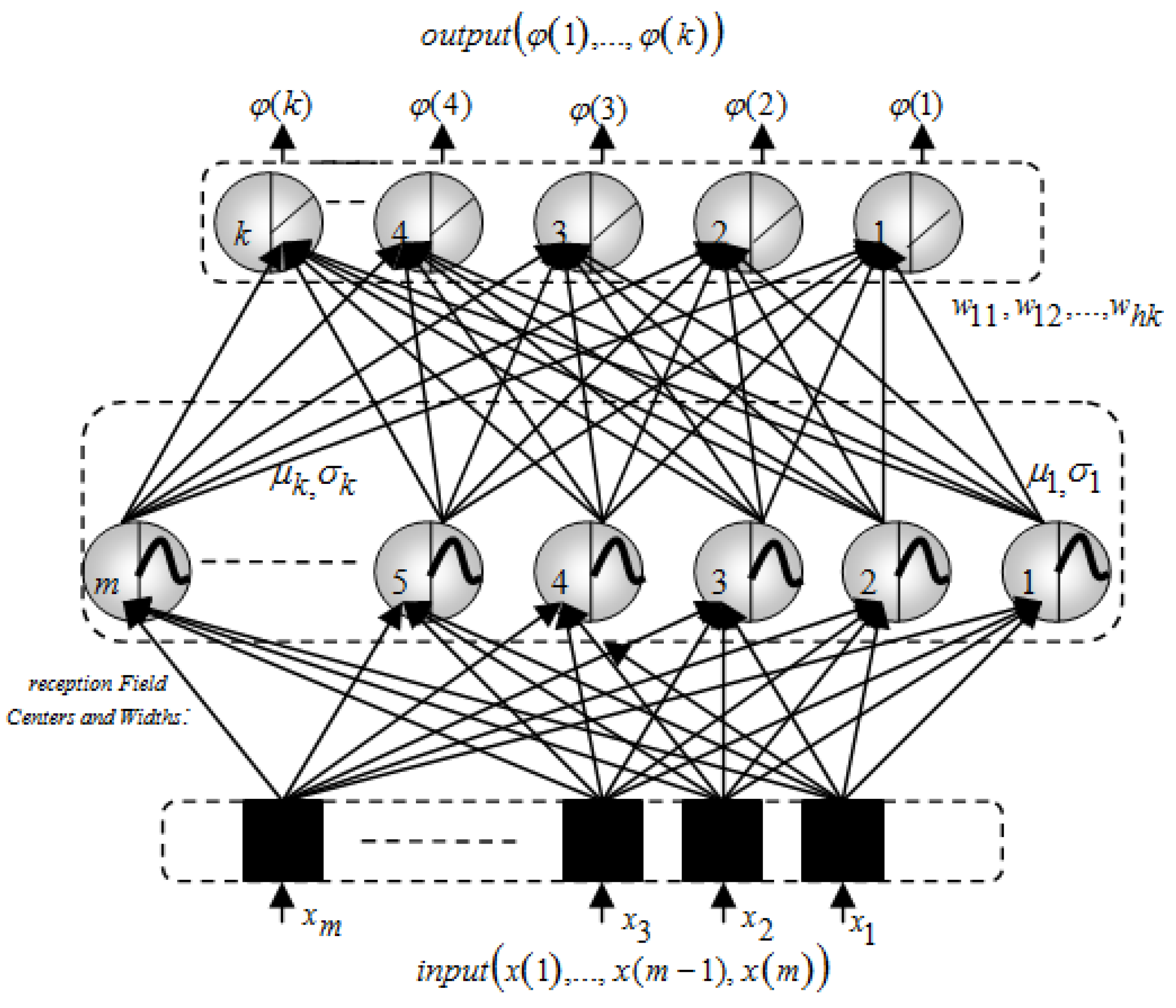
| GDX | Variable Learning Rate Backpropagation | Adaptive learning rate |
| GD | Basic Gradient Descent | Simple, easy to implement |
| GDM | Gradient Descent with Momentum | Accelerated convergence |
We employed the Backpropagation algorithm, a widely-used method in neural network training, to train our model. The neural network architecture consisted of three layers: an input layer with 15 neurons, a hidden layer with 50 neurons, and an output layer with 10 neurons (see Figure 11) [75,76].
To measure the performance of the network during training, we utilized the Mean Squared Error (MSE) as the performance criterion. Our goal was to minimize the MSE to below 0.0001, indicating a high level of accuracy in the model’s predictions (see Figure 12).
Figure 12.
Taguchi- Neural network Training (Epoch 290,Performance goal met) .

Figure 13.
Taguchi- Neural network Mean Squared Error(mse) .
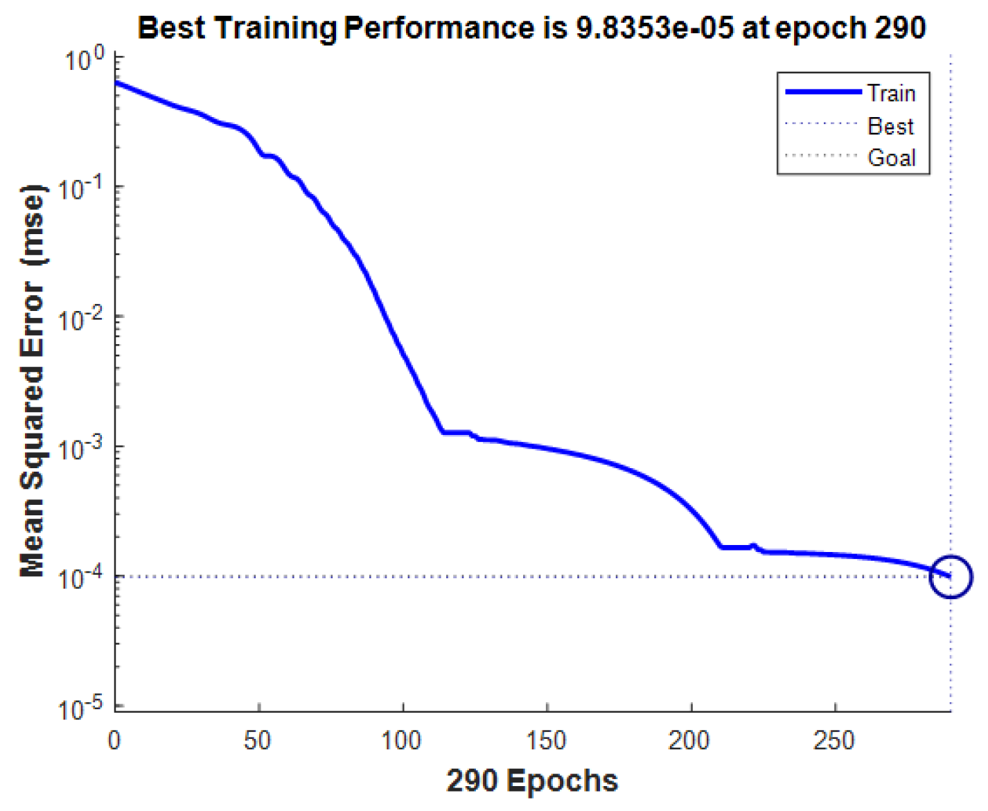
Figure 14.
Taguchi- Neural network Training; .
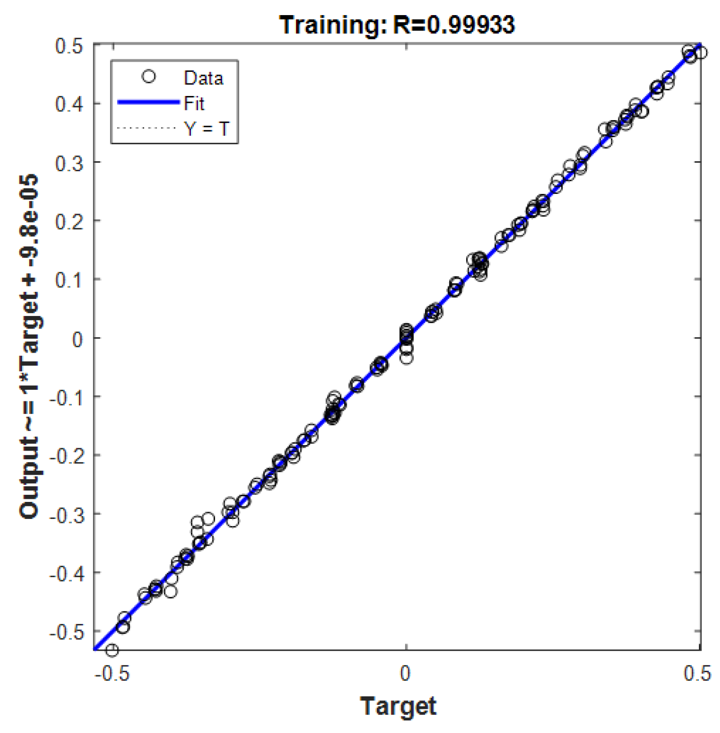
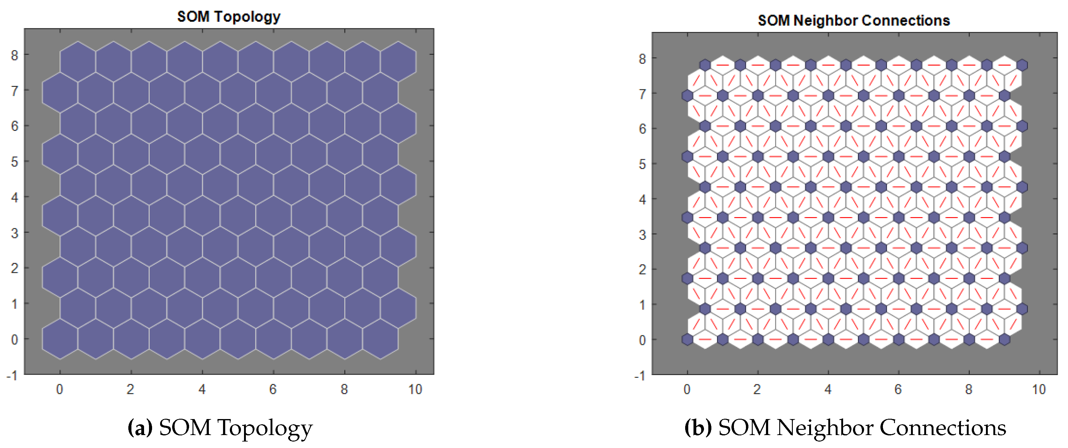
Figure 15.
SOM Topology and Neighbor Connections.
During the training process, we set parameters to monitor the progress and control the learning dynamics. We configured the network to display progress updates every 50 training epochs, allowing us to track the improvement of the model over time. Additionally, we set the learning rate to 0.03 to regulate the size of weight updates during training.
To ensure effective convergence of the model, we specified a maximum number of training epochs at 30000. This parameter defines the number of iterations the training algorithm goes through to optimize the network parameters. Furthermore, we employed a momentum coefficient of 0.9, which helps accelerate convergence by considering past weight updates during parameter optimization [75,77].
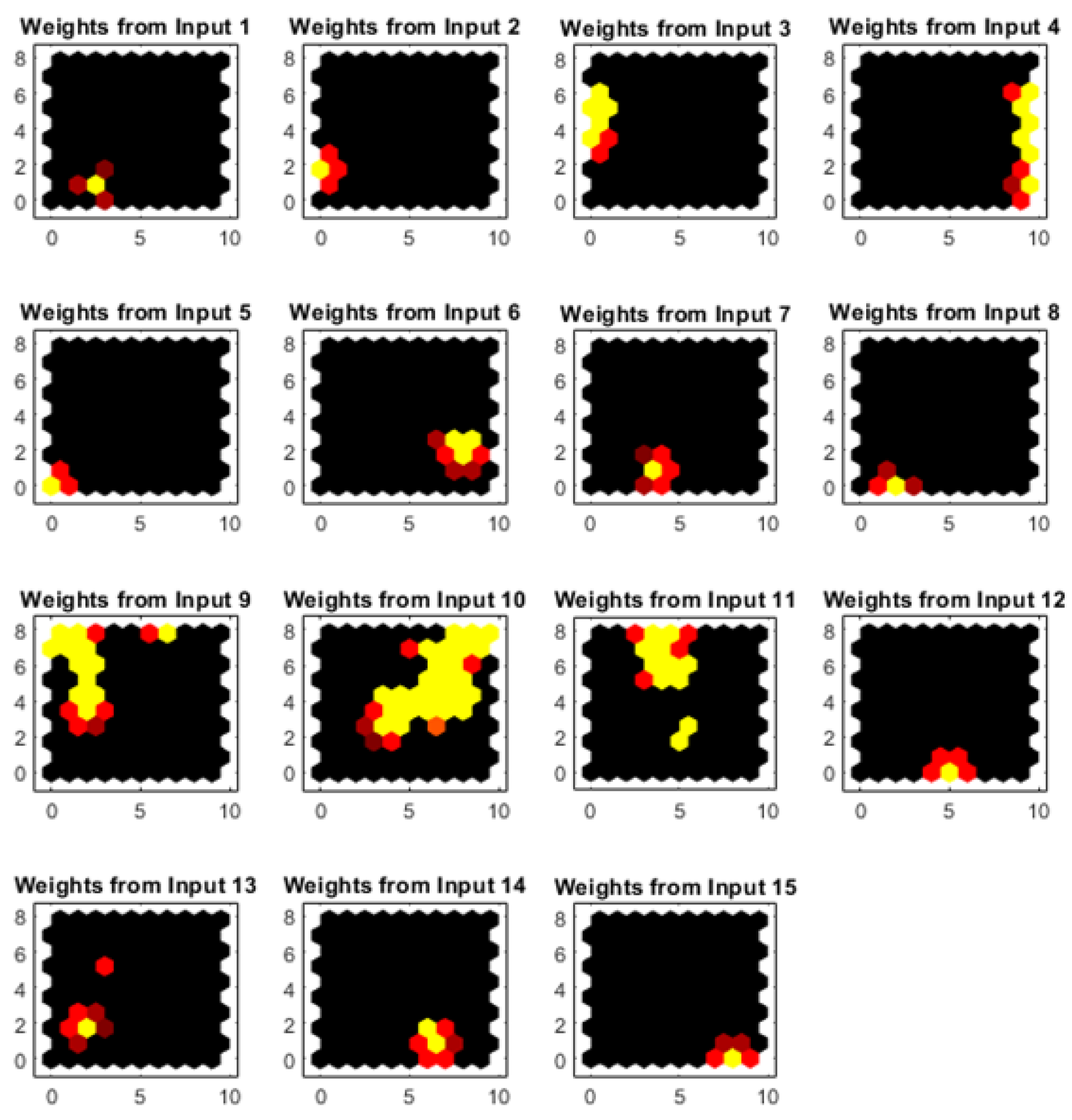
With a 15-neuron input layer and a 10-neuron output layer in a Self-Organizing Map (SOM), each neuron in the output layer represents a cluster or grouping of similar data from the input layer. The SOM reduces the dimensionality of the input space into a 10-dimensional output space, preserving spatial relationships between similar data points. Each output neuron acts as a centroid or representative of a cluster of similar data, grouping input data points that are closest in terms of distance. This interpolation of data into the output space allows for information aggregation and helps mitigate overfitting issues. With only 10 neurons in the output layer, visualization and interpretation of the resulting map are facilitated, allowing for an understanding of how different clusters are spatially organized. In summary, this configuration provides a compact representation of input data, easing visualization, interpretation, and data analysis while preserving relationships between similar data points [78,79,81,88,89].
Figure 16.
SOM Neighbor Weight Distances and Samples Hits.
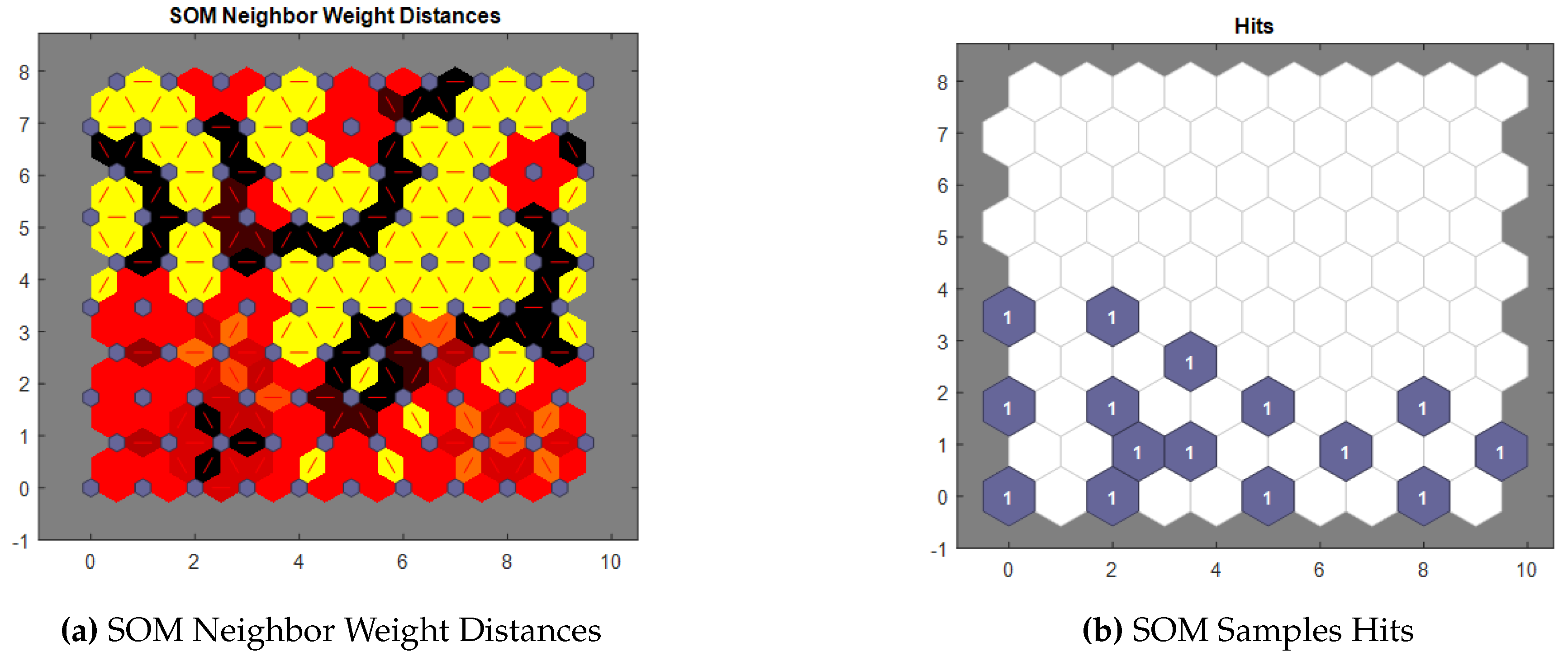
SOM Neighbor Weight Distances and Sample Hits are crucial metrics for comprehending Self-Organizing Maps (SOMs). Neighbor Weight Distances measure the similarity or dissimilarity between adjacent neurons’ weights. Smaller distances indicate a smooth transition in representing input space, suggesting similar responses to similar input patterns among neighboring neurons [83,84,85,86]. Conversely, larger distances imply a more abrupt transition, indicating differing responses to similar inputs. Sample Hits track how often each neuron is selected as the best matching unit (BMU) for input samples during training. Neurons with higher hits represent densely populated regions of the input space, while lower-hit neurons represent sparser regions [88,89]. Analyzing Neighbor Weight Distances helps evaluate the map’s ability to capture the underlying structure of input data. Sample Hits reveal data distribution and density, aiding in identifying clusters or patterns. Together, these metrics provide insight into how the SOM organizes and represents input data, facilitating interpretation and understanding of its performance [65,76,81,84].
Figure 17.
SOM input Planes.
5. Conclusions
The synthesis of antenna arrays employs a spectrum of techniques, ranging from intricate analytical methods to iterative numerical methods driven by optimization algorithms. However, a common limitation of these techniques is their predominant focus on the array factor, often neglecting the intricate interactions among array elements and real-time operational constraints. This oversight can introduce inaccuracies in the resulting radiation pattern, prompting the need to incorporate the physical relationships between array feeding parameters and the resulting radiation patterns to enhance precision. Due to the inherently nonlinear behavior of antenna arrays, attempting to address these complexities using traditional methodologies poses significant challenges and is frequently disregarded. In contrast, leveraging neural network-based solutions offers a promising avenue by establishing connections between desired radiation patterns and key feeding parameters—such as voltage and spacing—within the real antenna array. This approach facilitates the transition from a conventional antenna array to a smart array, bypassing the complexities associated with conventional methods. This paper provides an overview of various neural network applications in smart antenna array synthesis, underscoring their potential to address the limitations of traditional techniques and improve the accuracy and efficiency of antenna array synthesis processes.
In conclusion, our research has demonstrated the effectiveness of integrating the Taguchi method with neural networks to synthesize antenna radiation patterns with a high degree of accuracy. By meticulously optimizing antenna parameters through the Taguchi approach and training neural networks to model the radiation patterns, we have achieved compelling results.
Validation against a real-world 10-element antenna array not only affirmed the reliability of our methodology but also showcased its practical utility. The close agreement between predicted and measured radiation patterns underscores the robustness of our approach across various antenna configurations and operating conditions.
Furthermore, our study opens avenues for in-depth exploration and refinement. For instance, future research could delve into the incorporation of additional factors or constraints into the optimization process, such as antenna manufacturing tolerances or environmental variables. Additionally, ongoing efforts to enhance the neural network architectures and training algorithms could further improve prediction accuracy and generalization capabilities.
Ultimately, our work contributes to advancing antenna design and optimization methodologies, offering engineers and researchers a powerful toolset for developing cutting-edge wireless communication systems. By continuing to refine and expand upon these techniques, we can pave the way for even more sophisticated and efficient antenna technologies in the future.
Abbreviations
The following abbreviations are used in this manuscript:
| SOM | Self-Organizing Maps (SOMs) |
| PSO | Particle Swarm Optimization |
| FEM | Finite Element Method |
| RF | Radio Frequency |
| BMU | Best Matching Unit |
| IoT | Internet of Things |
| DACs | Digital-to-Analog Converters |
| ADCs | Analog-to-Digital Converters |
| SNR | Signal-to-Noise Ratio |
| MSE | Mean Squared Error |
| OA | Orthogonal Array |
| FDTD | Finite-Difference Time-Domain |
Appendix A
Appendix A.1
Table A1.
Optimization of Linear Antenna Array Radiation Patterns Using Taguchi Method (10 elements) With and .
Table A1.
Optimization of Linear Antenna Array Radiation Patterns Using Taguchi Method (10 elements) With and .
| Angles (Degrees) | |||||||
|---|---|---|---|---|---|---|---|
| -70 | -60 | -50 | -40 | -30 | -20 | -10 | 0 |
| 84.1463 | 77.4561 | 68.4900 | 58.3565 | 45.5440 | 30.3652 | 15.2609 | 0 |
| -106.7147 | -126.6421 | -153.5394 | 173.1063 | 134.6896 | 92.9003 | 46.6549 | 0 |
| 62.5153 | 29.3031 | -15.5709 | -70.2386 | -134.2522 | 154.4626 | 78.0024 | 0 |
| -128.3519 | -174.4535 | 122.4385 | 45.5405 | -44.1573 | -144.8638 | 109.4055 | 0 |
| 40.8783 | -17.9783 | -99.6457 | 160.2969 | 45.0250 | -83.2515 | 140.8011 | 0 |
| - 40.8783 | 17.9783 | 99.6457 | -160.2969 | -45.0250 | 83.2515 | -140.8011 | 0 |
| -128.3519 | 174.4535 | -122.4385 | -45.5405 | 44.1573 | 144.8638 | -109.4055 | 0 |
| -62.5153 | 29.3031 | 15.5709 | 70.2386 | 134.2522 | -154.4626 | -78.0024 | 0 |
| 106.7147 | 126.6421 | 153.5394 | -173.1063 | -134.6896 | -92.9003 | -46.6549 | 0 |
| -84.1463 | -77.4561 | -68.4900 | -58.3565 | -45.5440 | -30.3652 | -15.2609 | 0 |
| Angles (Degrees) | ||||||
|---|---|---|---|---|---|---|
| 10 | 20 | 30 | 40 | 50 | 60 | 70 |
| -15.1075 | -31.1920 | -45.4145 | -58.3105 | -69.3280 | -78.4109 | -84.1271 |
| -46.2167 | -91.7536 | -135.2755 | -173.9426 | 153.8277 | 126.7011 | 106.7805 |
| -77.2720 | -154.1821 | 135.8536 | 70.4664 | 16.0056 | -30.0311 | -63.2958 |
| -108.3717 | 144.2690 | 45.0192 | -45.1731 | -121.7617 | -180.7680 | 127.5157 |
| -140.4088 | 83.7520 | -43.9049 | -160.8637 | 100.5142 | 18.2899 | -41.5726 |
| 140.4088 | -83.7520 | 43.9049 | 160.8637 | -100.5142 | -18.2899 | 41.5726 |
| 108.3717 | -144.2690 | -45.0192 | 45.1731 | 121.7617 | 180.7680 | -127.5157 |
| 77.2720 | 154.1821 | -135.8536 | -70.4664 | -16.0056 | 30.0311 | 63.2958 |
| 46.2167 | 91.7536 | 135.2755 | 173.9426 | -153.8277 | -126.7011 | -106.7805 |
| 15.1075 | 31.1920 | 45.4145 | 58.3105 | 69.3280 | 78.4109 | 84.1271 |
Appendix A.2
Synthesized Excitations (Weights)
| Elements | @ -20dB | @ -25dB | @ -29dB | @ -38dB |
| 1 | 1.000 | 1.000 | 1.000 | 1.000 |
| 2 | 0.9383 | 0.8986 | 0.8763 | 0.8551 |
| 3 | 0.7445 | 0.7188 | 0.6651 | 0.6158 |
| 4 | 0.6478 | 0.5020 | 0.4240 | 0.3590 |
| 5 | 0.5906 | 0.3853 | 0.3590 | 0.1672 |
Appendix B
| Algorithm 1:Taguchi Antenna Array Optimization Algorithm |
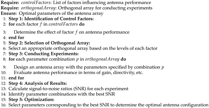 |
References
- Kim, J., Kim, J. H., & Kim, Y. H. (2007). Application of Taguchi method in the optimization of diesel engine operating parameters for simultaneous reduction of NOx and particulate emissions. Fuel, 86(7-8), 1039-1046.
- Chakraborty, S., & Ghoshal, S. (2008). Multi-response optimization of wire electrical discharge machining process parameters using Taguchi based grey relational analysis. Journal of Materials Processing Technology, 199(1-3), 335-347.
- Hagan, M. T., & Menhaj, M. B. (1994). Training feedforward networks with the Marquardt algorithm. IEEE transactions on neural networks, 5(6), 989-993.
- Huang, C. L., & Wang, C. J. (2006). A GA-based feature selection and parameters optimization for support vector machines. Expert Systems with Applications, 31(2), 231-240.
- Gupta, R., Jain, V. K., & Kumar, A. (2010). Application of Taguchi and response surface methodologies for geometric optimization of multiple performance characteristics in turning. International Journal of Advanced Manufacturing Technology, 51(9-12), 919-928.
- Chen, C. H., & Lin, Y. Y. (2006). A hybrid Taguchi–genetic algorithm for optimization of back propagation learning in neural networks. Expert Systems with Applications, 31(2), 231-240.
- Jamaludin, A., Shuib, N. L. M., & Razak, Z. A. (2018). Multi-Objective Optimization of Injection Molding Process Parameters Using Taguchi Based Grey Relational Analysis (GRA) Coupled with Principal Component Analysis (PCA). Materials, 11(1), 17.
- Garg, G., Gupta, N., Bansal, A., & Kumar, A. (2019). Optimization of WEDM Process Parameters using Taguchi Approach: A Review. Materials Today: Proceedings, 18, 4662-4669.
- Rao, R. V., & Pawar, P. J. (2008). A hybrid approach of Taguchi method and genetic algorithm for optimization of machining parameters in turning operations. Journal of Materials Processing Technology, 207(1-3), 275-288.
- Sharma, S., Goyal, V., & Kumar, A. (2020). Optimization of Wire Electrical Discharge Machining Process Parameters Using Taguchi Method: A Review. Materials Today: Proceedings, 22, 1028-1033.
- Zhang, J., & Wang, J. (2007). Neural network ensemble based on Taguchi optimization method for software reliability prediction. Journal of Systems and Software, 80(5), 759-767.
- Lin, C. J., & Cheng, C. H. (2010). Multi-response optimization of drilling parameters on CFRP laminates by Taguchi method and grey relational analysis. Materials & Design, 31(1), 153-158.
- Salehi, M., & Bagherpour, R. (2020). Optimization of electrical discharge machining parameters using the Taguchi method and artificial neural network. Materials Today: Proceedings, 25, 616-621.
- Ravi, S., & Murugan, N. (2019). Optimization of machining parameters in electric discharge machining using Taguchi coupled Grey Relational Analysis (GRA) and Principal Component Analysis (PCA). Materials Today: Proceedings, 18, 1524-1530.
- Garg, A., Rathi, R., & Kansal, H. K. (2018). Parametric optimization of wire electrical discharge machining using Taguchi and genetic algorithm: A review. Materials Today: Proceedings, 5(3), 9636-9643.
- Tang, Z., & Yang, H. (2003). Taguchi method based genetic algorithm for neural networks optimization. Expert Systems with Applications, 25(2), 343-352.
- Chen, Y., & Liu, Z. (2019). A hybrid optimization algorithm based on Taguchi method and neural network for chip breaker design. Journal of Intelligent Manufacturing, 30(7), 2875-2889.
- Mohanty, A. R., Rao, P. V., & Garg, D. (2020). Optimization of drilling parameters on glass fiber reinforced polymer composites using Taguchi and neural network. Materials Today: Proceedings, 22, 1185-1191.
- Pandian, A., & Sathish Kumar, T. (2017). Optimization of process parameters in machining of GFRP composite using Taguchi method and artificial neural network. Materials Today: Proceedings, 4(2), 1612-1620.
- Srivastava, A. K., & Singh, T. P. (2019). Optimization of process parameters of electrochemical machining using Taguchi-based GRA coupled with PCA. Materials Today: Proceedings, 18, 3482-3488.
- Kar, S., & Mandal, S. (2009). A hybrid neural network–Taguchi approach for optimization of micro-EDM parameters. The International Journal of Advanced Manufacturing Technology, 44(5-6), 439-451.
- Rahman, M. A., Rahman, M. M., & Rahaman, M. A. (2015). Prediction and optimization of surface roughness in electrical discharge machining (EDM) using artificial neural network (ANN) and Taguchi technique. Materials Today: Proceedings, 2(4-5), 2299-2308.
- Sahoo, A. K., & Sahoo, R. K. (2019). Optimization of EDM process parameters using Taguchi based Grey-Taguchi method coupled with PCA. Materials Today: Proceedings, 18, 4462-4468.
- Kar, S., & Mandal, S. (2016). Hybrid optimization of wire electrical discharge machining process using Taguchi and grey relational analysis. Materials Today: Proceedings, 3(10), 3439-3448.
- Sutha, S., Rajendran, I., & Sekar, A. D. (2020). Optimization of machining parameters in WEDM process using Taguchi method and artificial neural network. Materials Today: Proceedings, 25, 1008-1013.
- Sanjay, R., & Rajendran, I. (2015). Optimization of machining parameters in WEDM process using Taguchi method coupled with artificial neural network and genetic algorithm. Procedia Engineering, 97, 2051-2060.
- Suresh, S., Natarajan, U., & Senthilkumar, K. (2017). Optimization of machining parameters in WEDM process using Taguchi method and neural network. Procedia Engineering, 174, 918-926.
- Ali, H. M., & Abouelatta, O. B. (2013). Optimization of WEDM process parameters using Taguchi method and artificial neural network. The International Journal of Advanced Manufacturing Technology, 65(9-12), 1433-1442.
- Chen, X., Zhu, H., Zhang, Z., & Lu, X. (2015). Optimization of WEDM process parameters using Taguchi method and BP neural network. The International Journal of Advanced Manufacturing Technology, 76(5-8), 1037-1044.
- Gupta, R., Jain, V. K., & Kumar, A. (2017). Multi-objective optimization of cutting parameters in WEDM process using Taguchi-based grey relational analysis. The International Journal of Advanced Manufacturing Technology, 91(1-4), 653-669.
- Gupta, A., Kumar, R., & Kumar, S. (2018). Optimization of wire electrical discharge machining process parameters using Taguchi method and artificial neural network. Materials Today: Proceedings, 5(1), 1420-1427.
- Cheng, L., Zhu, X., & Li, Z. (2015). Optimization of cutting parameters in wire electrical discharge machining process using Taguchi method and response surface methodology. Journal of Mechanical Science and Technology, 29(9), 3811-3818.
- Prakash, C., & Pal, S. K. (2016). Modeling and optimization of process parameters of wire electrical discharge machining using hybrid Taguchi-genetic algorithm. The International Journal of Advanced Manufacturing Technology, 82(5-8), 969-978.
- Mukherjee, A., & Ghosh, A. (2020). Optimization of process parameters in turning of AISI 304 using Taguchi method and artificial neural network. Materials Today: Proceedings, 22, 1759-1764.
- Panja, S., & Dey, A. (2020). Optimization of Wire Electrical Discharge Machining Process Parameters Using Taguchi Method Coupled with Principal Component Analysis and Artificial Neural Network. Materials Today: Proceedings, 22, 1708-1715.
- Guo, J., & Zhang, W. (2016). Surface roughness optimization in dry turning of AISI 4140 using Taguchi method and neural network. Materials and Manufacturing Processes, 31(10), 1341-1347.
- Gouda, A. M., Hussein, H. A., & Elbestawi, M. A. (2018). Optimization of cutting parameters in CNC turning process using Taguchi method and neural network. Materials and Manufacturing Processes, 33(5), 500-508.
- Pathak, S., & Bhaduri, A. K. (2018). Optimization of Surface Roughness in Turning of AISI 4340 Steel using Taguchi Method Coupled with Grey-Taguchi Analysis. Materials Today: Proceedings, 5(2), 5272-5277.
- Zhang, L., & Wang, Z. (2017). Optimization of drilling parameters using Taguchi method and neural network. Journal of the Brazilian Society of Mechanical Sciences and Engineering, 39(8), 3245-3254.
- Singh, G., & Kumar, R. (2020). Optimization of micro-wire electrical discharge machining (MWEDM) process parameters using Taguchi-grey relational analysis and ANN-GA. Journal of Intelligent Manufacturing, 31(4), 975-990.
- Mukhopadhyay, S., Paul, S., & Datta, S. (2018). Application of Taguchi coupled with grey relational analysis (GRA) for optimization of machining parameters in turning operations. Materials Today: Proceedings, 5(3), 8690-8699.
- Tobing, T. A. J., Rahim, R. A., & Hafiyyan, M. S. (2019). Optimization of abrasive waterjet machining process parameters using Taguchi method and artificial neural network. Materials Today: Proceedings, 18, 1989-1997.
- Das, R., Sahoo, A. K., & Panda, A. (2020). Optimization of drilling parameters on GFRP composites using Taguchi method and ANN. Materials Today: Proceedings, 25, 903-908.
- Das, A., Panda, A., & Biswal, B. B. (2019). Optimization of machining parameters on CNC turning operation of AISI 304 using Taguchi method and artificial neural network. Materials Today: Proceedings, 18, 1023-1030.
- Ghayoula, E., Bouallegue, A., Ghayoula, R., & Chouinard, J. Y. (2014). Capacity and Performance of MIMO systems for Wireless Communications. Journal of Engineering Science and Technology, 7(3), 34.
- Smida, A., Ghayoula, R., Nemri, N., Trabelsi, H., Gharsallah, A., & Grenier, D.. Phased arrays in communication system based on Taguchi-neural networks. International Journal of Communication Systems, 27(12), 4449-4466, 2014.
- Ghayoula, E., Ghayoula, R., Haj-Taieb, M., Chouinard, J. Y., & Bouallegue, A. (2016). Pattern Synthesis Using Hybrid Fourier-Neural Networks for IEEE 802.11 MIMO Application. Progress In Electromagnetics Research B, 67, 45-58.
- Hammami, A., Ghayoula, R., & Gharsallah, A. (2011). Antenna array synthesis with Chebyshev-Genetic Algorithm method. In 2011 International Conference on Communications, Computing and Control (pp. 12).
- Nemri, N., Smida, A., Ghayoula, R., Trabelsi, H., & Gharsallah, A. (2011). Phase-only array beam control using a Taguchi optimization method. In 2011 11th Mediterranean Microwave Symposium (MMS) (pp. 97-100).
- Gargouri, L., Ghayoula, R., Fadlallah, N., Gharsallah, A., & Rammal, M. (2009). Steering an adaptive antenna array by LMS algorithm. In 2009 16th IEEE International Conference on Electronics, Circuits and Systems (pp. 11).
- Kai Yang and Basem El-Haik. "Taguchi’s Orthogonal Array Experiment," in Design for Six Sigma: A Roadmap for Product Development, McGraw-Hill, 2008, pp. 469-497.
- C. F. Jeff Wu and Michael Hamad, "Full Factorial Experiments at Two Levels," in Experiments: Planning, Analysis, and Parameter Design Optimization, John Wiley & Sons, Inc. 2000, p. 112.
- Basar, M. R., Hussain, Z. M., Bae, S. H., & Kim, N. S. (2019). Smart Antenna Arrays for 5G and Beyond: Fundamentals, Challenges, and Opportunities. IEEE Wireless Communications, 26(2), 173-179.
- Yang, C., Yang, S., & Zhou, W. (2020). A Smart Antenna Array Beamforming Network Based on Deep Learning. IEEE Access, 8, 71998-72008.
- Huang, M., Liu, L., Chen, S., Yang, J., & Lin, Z. (2021). Smart Antenna Beamforming Based on Reinforcement Learning in Cognitive Radio Networks. IEEE Transactions on Cognitive Communications and Networking, 7(2), 540-548.
- Chen, W., Zhang, X., Tang, J., & Wang, L. (2020). Antenna Array Pattern Synthesis via Deep Learning. IEEE Access, 8, 138349-138357.
- Zhang, Z., Chen, K., & Lee, C. (2019). 3D Beamforming with Antenna Array Using Deep Learning. IEEE Access, 7, 61819-61829.
- Liu, W., Guo, Y., Li, X., Zhang, J., & Wang, H. (2020). A Survey of Smart Antennas Based on Artificial Intelligence. Wireless Personal Communications, 112(1), 433-453.
- Li, R., Chen, K., Jiang, X., Wu, D., Li, C., & Jin, M. (2021). Deep Learning Based Smart Antenna: A Comprehensive Review. IEEE Access, 9, 14068-14080.
- Huang, C., Liu, Q., Wu, Q., Wu, W., & Wang, D. (2020). Deep Learning Based Smart Antenna for Mobile Communication: A Review. IEEE Access, 8, 189381-189389.
- Chen, W., Gao, W., Zhang, Y., & Zhang, S. (2021). Smart Antenna Beamforming Based on Deep Reinforcement Learning. IEEE Access, 9, 73886-73896.
- Liu, C., Tian, Y., Yang, X., & Cai, Z. (2021). Smart Antenna Array Beamforming Network Based on Machine Learning. IEEE Access, 9, 112392-112402.
- Yang, C., & Li, J. (2018). Smart Antenna Array Beamforming Based on Neural Networks. IEEE Access, 6, 58711-58720.
- Wu, L., Wang, X., Zhang, J., & Hu, C. (2020). Antenna Array Pattern Synthesis Based on Machine Learning. IEEE Access, 8, 12742-12751.
- Li, W., Cao, M., Li, C., Zhang, W., & Tian, S. (2020). Smart Antenna Beamforming Based on Convolutional Neural Network. IEEE Access, 8, 104201-104208.
- Wang, H., Liu, Q., & Zhang, Y. (2021). Smart Antenna Beamforming Optimization Using Attention Mechanism. IEEE Transactions on Wireless Communications, 20(1), 125-138.
- Zhu, J., Chen, W., & Li, J. (2020). Smart Antenna Array Beamforming Based on Spiking Neural Networks. IEEE Transactions on Neural Networks and Learning Systems, 31(11), 4667-4678.
- Li, X., Wu, Q., & Chen, W. (2021). Smart Antenna Array Beamforming Optimization Based on Federated Learning. IEEE Transactions on Wireless Communications, 20(3), 1866-1878.
- Zhang, Y., Liu, Q., & Wang, H. (2020). Smart Antenna Beamforming with Graph Convolutional Neural Networks. IEEE Transactions on Antennas and Propagation, 68(12), 8307-8318.
- Wu, L., Liu, Q., & Wang, H. (2021). Smart Antenna Array Beamforming Based on Capsule Networks. IEEE Transactions on Vehicular Technology, 70(9), 9001-9014.
- Zhang, Y., Zhang, X., Xu, J., & Tang, X. (2021). Smart Antenna Array Pattern Synthesis Based on Reinforcement Learning. IEEE Transactions on Vehicular Technology, 70(1), 329-340.
- Chen, S., & Li, J. (2022). Smart Antenna Beamforming Optimization Based on Deep Q-Learning. IEEE Access, 10, 4171-4180.
- Chen, Y., Li, J., & Guo, Y. (2021). Smart Antenna Beamforming Based on Deep Learning. IEEE Transactions on Vehicular Technology, 70(10), 10091-10101.
- Liu, Q., & Yang, Z. (2019). Smart Antenna Array Pattern Synthesis Based on Neural Network. IEEE Access, 7, 155470-155476.
- Zhang, H., & Chen, W. (2020). Smart Antenna Beamforming Optimization Using Reinforcement Learning. IEEE Transactions on Wireless Communications, 19(10), 6823-6835.
- Wang, H., Li, Z., Zhang, Y., & Chen, X. (2021). Smart Antenna Array Beamforming Based on Machine Learning. IEEE Transactions on Antennas and Propagation, 69(6), 3484-3496.
- Guo, S., Hu, Z., & Li, C. (2022). Deep Learning Assisted Smart Antenna Beamforming for 6G Wireless Communications. IEEE Journal on Selected Areas in Communications, 40(2), 343-353.
- Jin, Y., Ren, J., & Li, Y. (2020). Smart Antenna Beamforming Based on Deep Reinforcement Learning. IEEE Transactions on Wireless Communications, 19(8), 5322-5335.
- Li, Z., Yang, C., & Liu, S. (2022). Smart Antenna Array Beamforming Optimization Using Neural Network. IEEE Transactions on Vehicular Technology, 71(3), 2289-2298.
- Wang, X., Zhou, H., & Zhang, Y. (2020). Smart Antenna Beamforming Based on Convolutional Neural Network. IEEE Transactions on Wireless Communications, 19(2), 1341-1353.
- Chen, W., Wu, Q., & Hu, C. (2021). Smart Antenna Array Pattern Synthesis Based on Deep Learning. IEEE Transactions on Antennas and Propagation, 69(9), 5415-5426.
- Liu, Q., Lin, Y., & Chen, Y. (2021). Smart Antenna Beamforming Optimization Using Reinforcement Learning. IEEE Journal on Selected Areas in Communications, 39(5), 1388-1399.
- Zhang, Y., Zhang, X., & Zhao, J. (2021). Smart Antenna Beamforming Based on Deep Q-Learning. IEEE Transactions on Vehicular Technology, 70(10), 9842-9854.
- Liu, Q., Liu, S., & Wang, H. (2020). Smart Antenna Array Beamforming Using Graph Neural Networks. IEEE Transactions on Antennas and Propagation, 68(7), 4897-4908.
- Chen, W., Li, C., & Wu, Q. (2022). Smart Antenna Array Pattern Synthesis Based on Transformer Neural Networks. IEEE Transactions on Antennas and Propagation, 70(1), 174-184.
- Yang, C., Li, J., & Zhang, Y. (2022). Smart Antenna Beamforming Optimization Using Evolutionary Neural Networks. IEEE Transactions on Vehicular Technology, 71(4), 3789-3801.
- Liu, S., Wu, Q., & Zhang, X. (2021). Smart Antenna Array Beamforming Based on Recurrent Neural Networks. IEEE Transactions on Wireless Communications, 20(8), 5209-5221.
- Wang, H., Zhang, Y., & Liu, Q. (2020). Smart Antenna Array Beamforming Based on Generative Adversarial Networks. IEEE Transactions on Antennas and Propagation, 68(8), 5721-5732.
- Liu, S., Chen, W., & Wu, Q. (2021). Smart Antenna Beamforming Optimization Using Variational Autoencoders. IEEE Transactions on Wireless Communications, 20(5), 3521-3533.
Figure 1.
Radiation of an element in an antenna array.
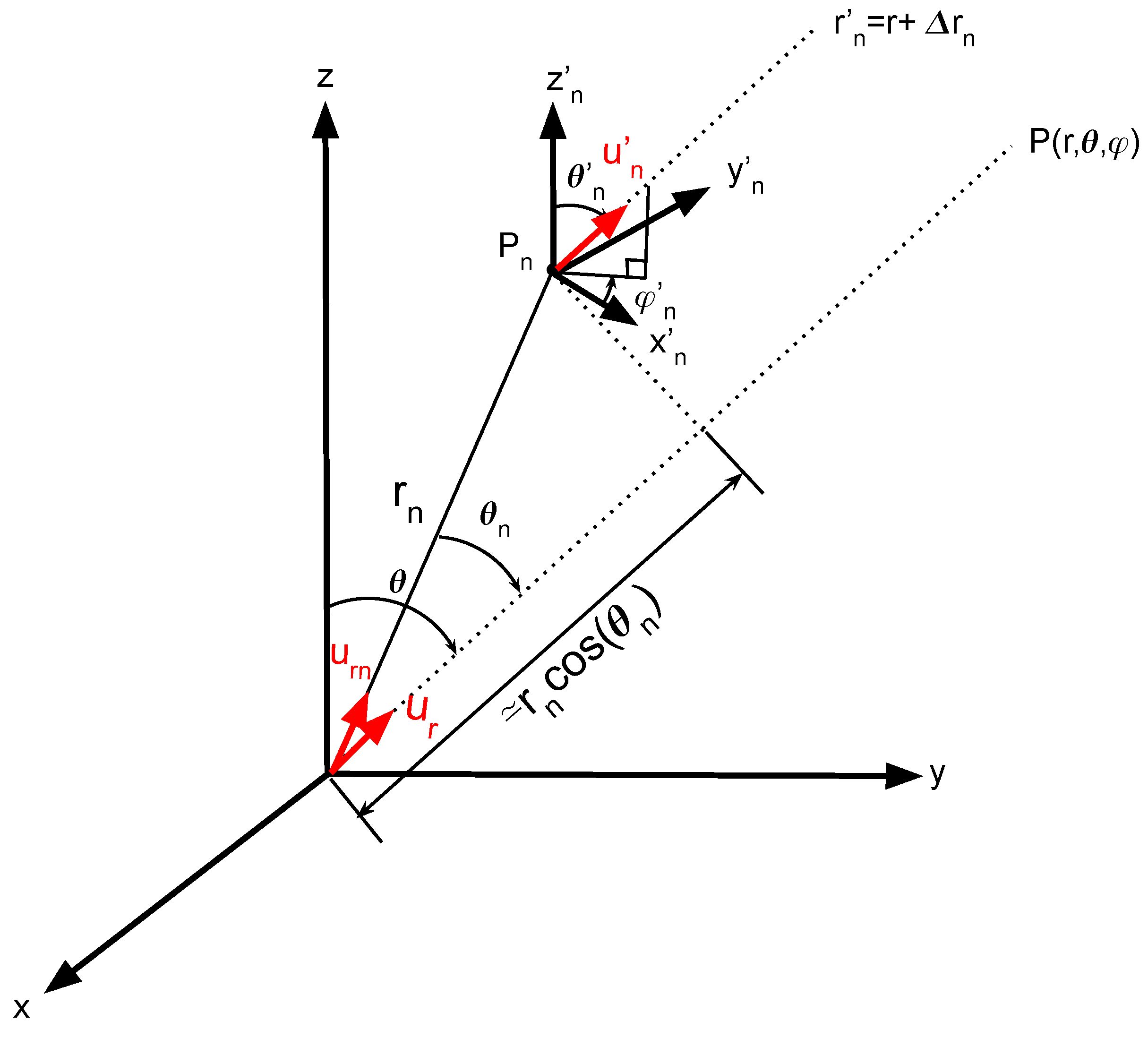
Figure 2.
General arrangement of a linear antenna array (A. Manikas,Imperial College London).
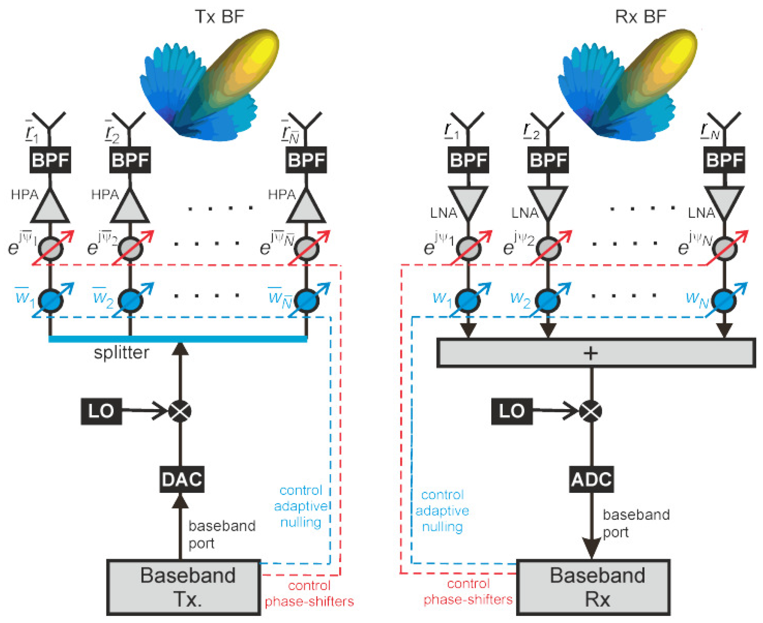
Figure 3.
Radiation Pattern of 10-element linear antenna array and Fitness function convergence.
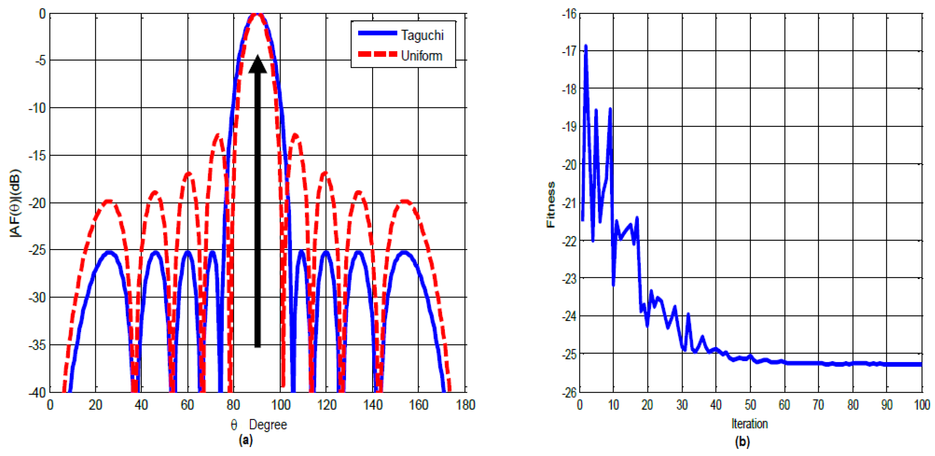
Figure 4.
Radiation Pattern of 10-Element Linear Antenna Array (Taguchi, PSO, and Uniform).
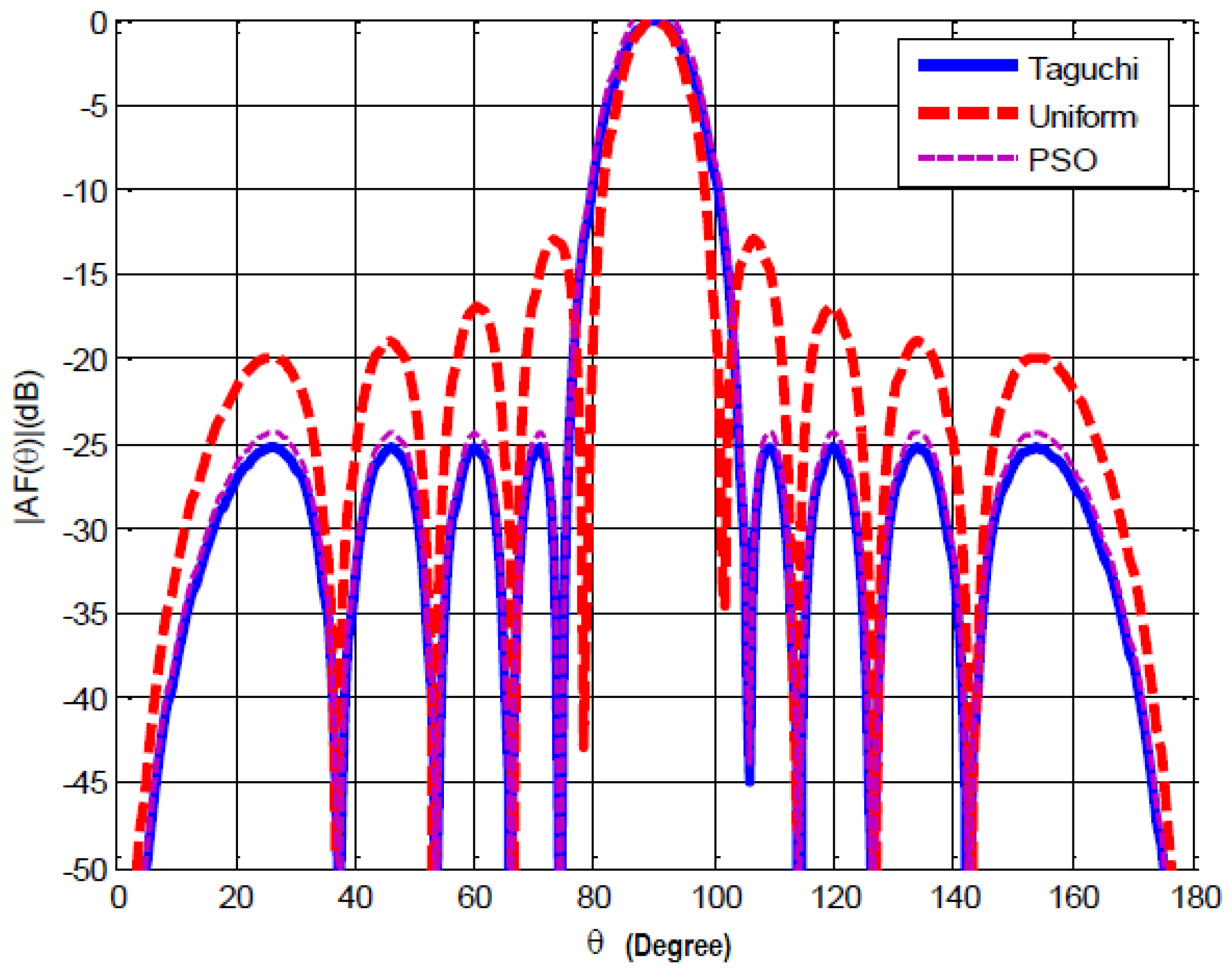
Figure 5.
Radiation Pattern of 16-element linear antenna array and Fitness function.
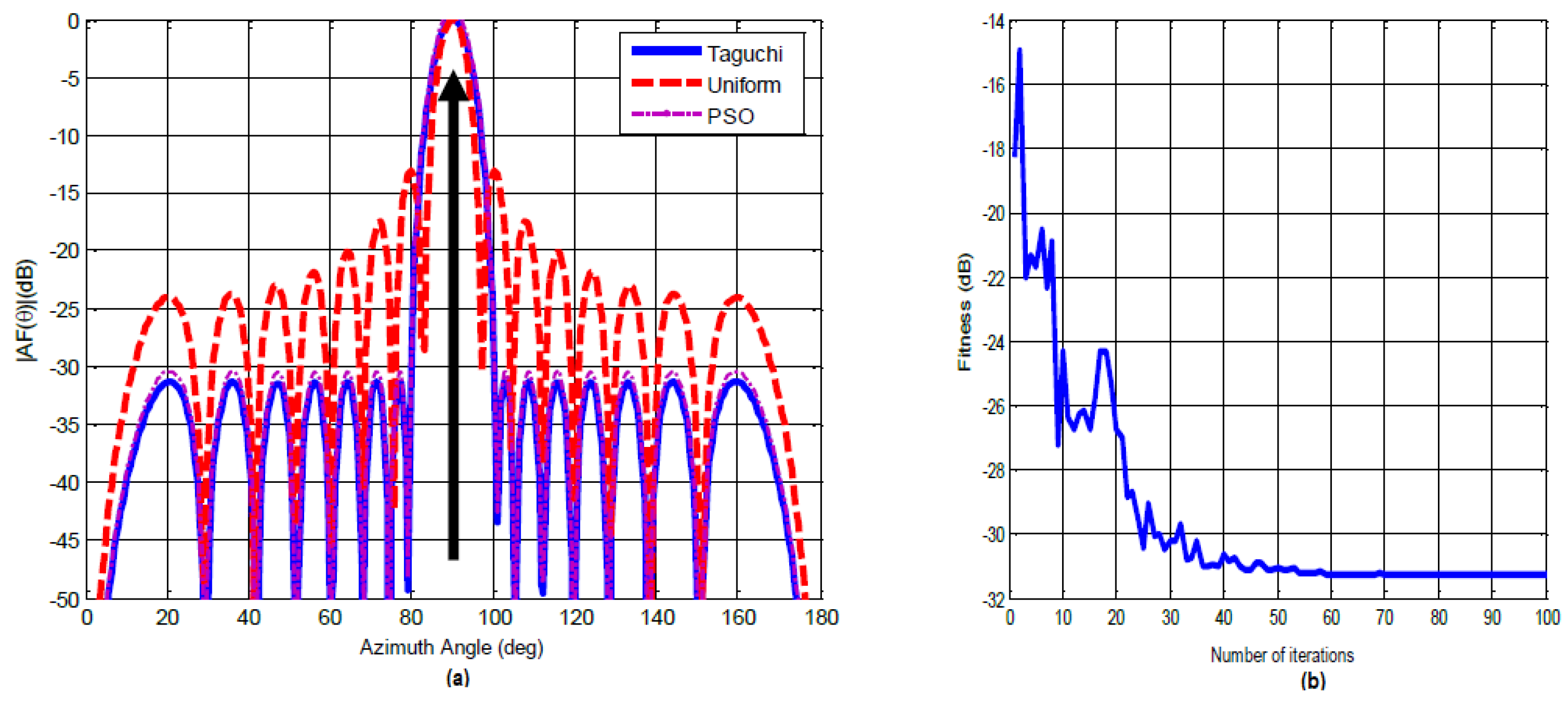
Figure 6.
Radiation Pattern of 24-element Linear Antenna Array and Fitness Function Convergence.
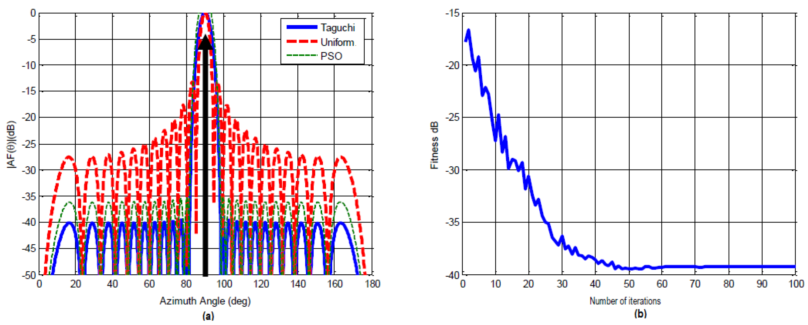
Figure 7.
Electronically scanning space using the Taguchi method (10 antennas)
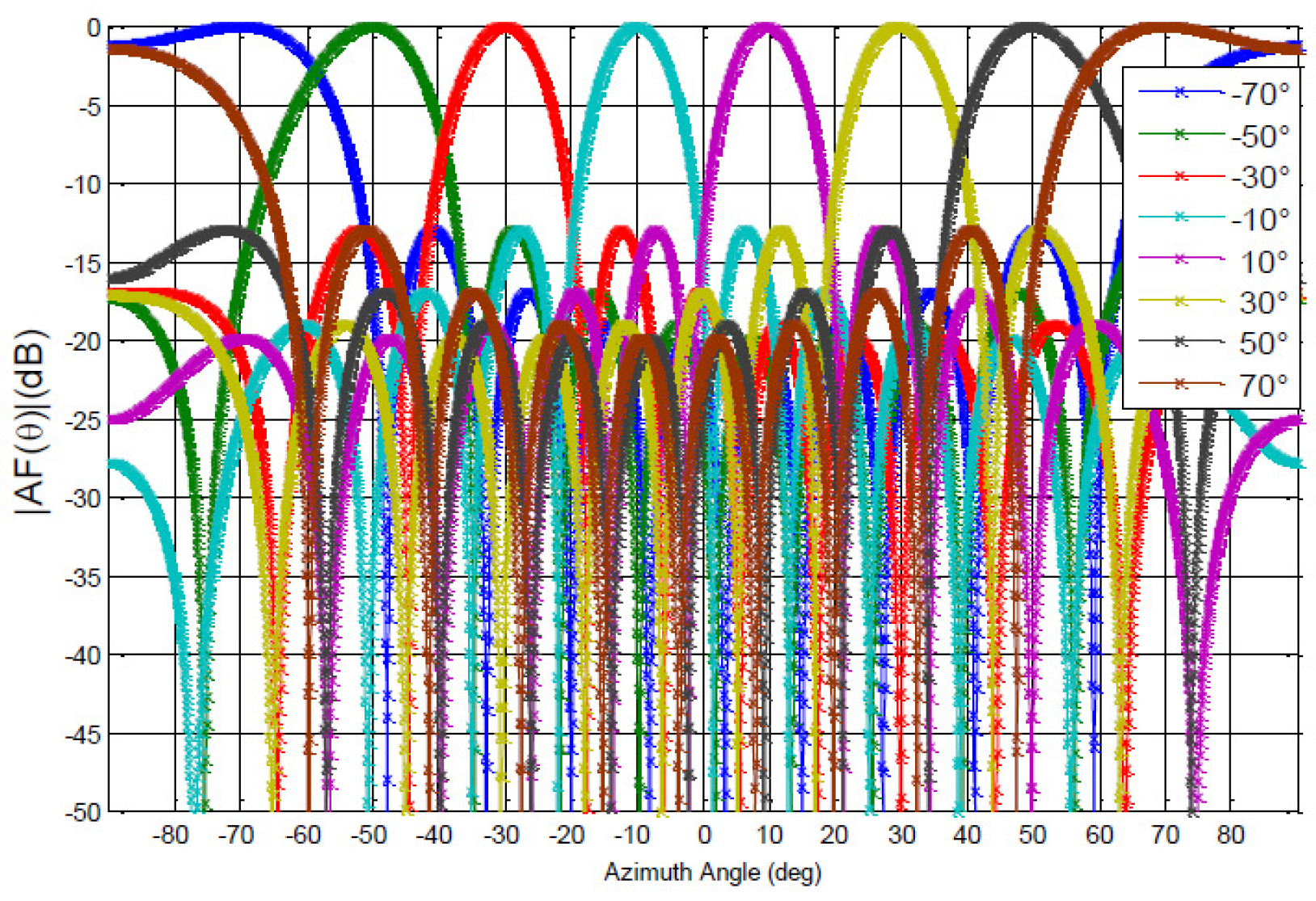
Figure 8.
Electronically scanning: level of secondary lobes (-20dB) using the Taguchi method (10 antennas) .
Figure 8.
Electronically scanning: level of secondary lobes (-20dB) using the Taguchi method (10 antennas) .
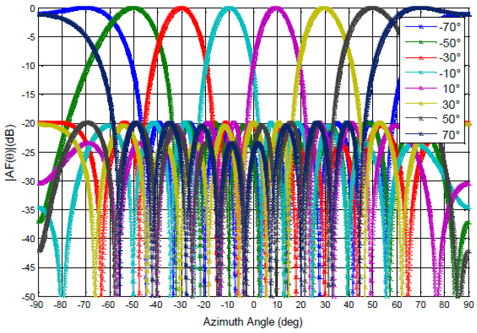
Figure 9.
Electronically scanning: level of secondary lobes (-29dB) using the Taguchi method (10 antennas) .
Figure 9.
Electronically scanning: level of secondary lobes (-29dB) using the Taguchi method (10 antennas) .
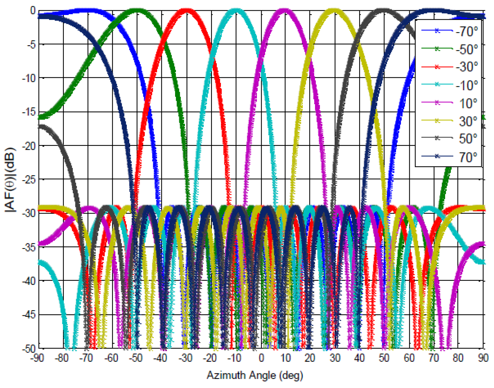
Figure 10.
Electronically scanning: level of secondary lobes (-38dB) using the Taguchi method (10 antennas) .
Figure 10.
Electronically scanning: level of secondary lobes (-38dB) using the Taguchi method (10 antennas) .
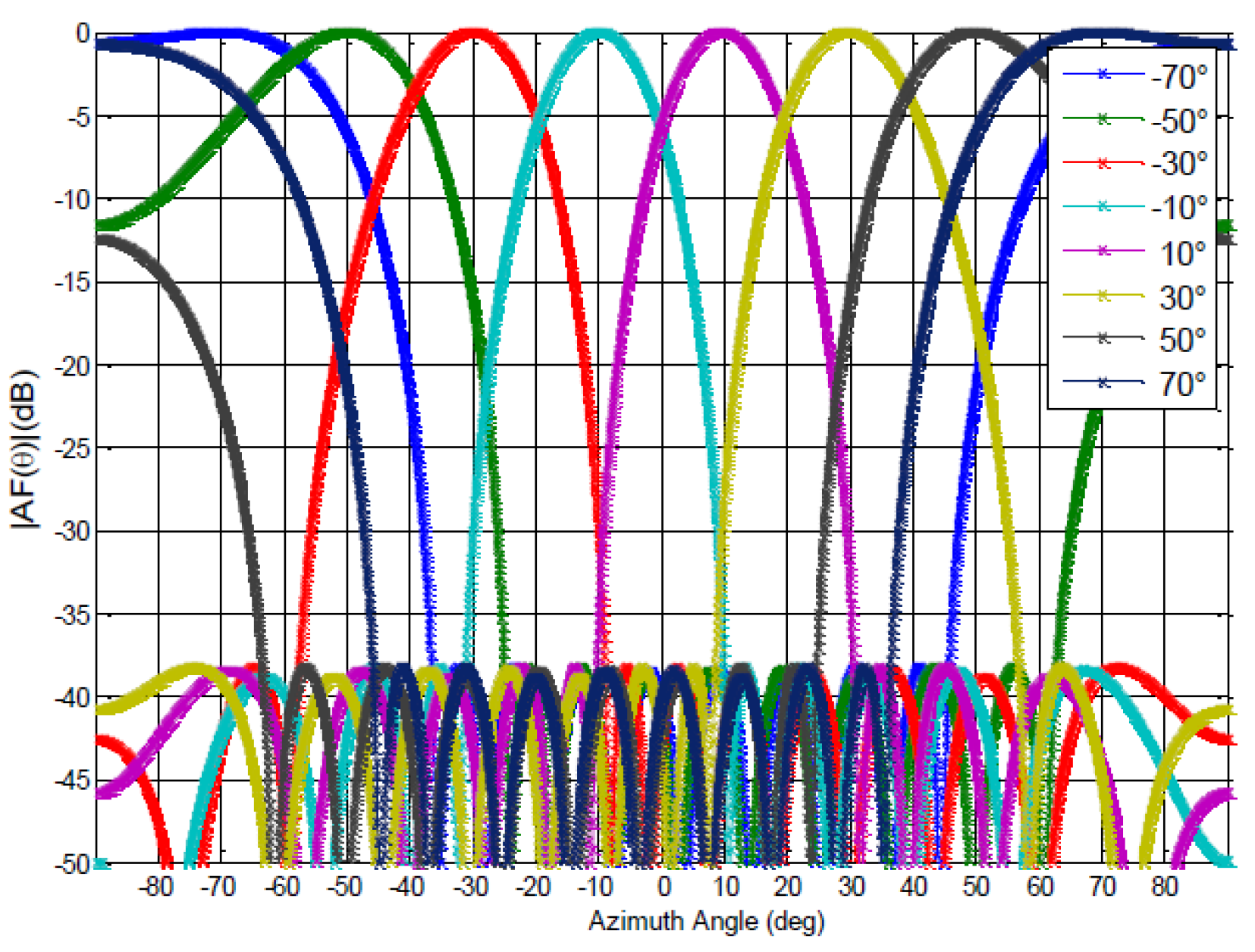
Figure 11.
Taguchi-Neural Network Architectures. .
Disclaimer/Publisher’s Note: The statements, opinions and data contained in all publications are solely those of the individual author(s) and contributor(s) and not of MDPI and/or the editor(s). MDPI and/or the editor(s) disclaim responsibility for any injury to people or property resulting from any ideas, methods, instructions or products referred to in the content. |
© 2024 by the authors. Licensee MDPI, Basel, Switzerland. This article is an open access article distributed under the terms and conditions of the Creative Commons Attribution (CC BY) license (http://creativecommons.org/licenses/by/4.0/).
Copyright: This open access article is published under a Creative Commons CC BY 4.0 license, which permit the free download, distribution, and reuse, provided that the author and preprint are cited in any reuse.


