
Submitted:
16 April 2024
Posted:
16 April 2024
You are already at the latest version
Abstract
Solar energetic particles (SEPs) are bursts of high-energy particles that originate from the Sun and can last for hours or even days. The aim of this study is to understand how the characteristics of energetic particles was affected by the characteristic parameters of corotating interaction regions (CIRs). In particular, the particle intensity distribution with time and space in different CIRs are studied. The propagation and acceleration of particles are described by the focused transport equation (FTE). We used a three-dimensional magnetohydrodynamic (MHD) model to simulate the background field including CIRs. By changing the inner boundary conditions, we constructed CIRs with different solar wind speeds, angles between the polar axis and rotation axis, and the azimuthal widths of the fast streams. Impulsive particles are injected at the inner boundary. We then study the SEPs in different backgrounds. The results show that the CIR widths are related to the solar wind speed, tilt angles, and the azimuthal widths of the fast stream. The acceleration of particles in the reverse and forward compression regions is mainly influenced by the solar wind speed difference and the slow solar wind speed, respectively. Particles with lower energy (sub-MeV) are more sensitive to the parameters of CIRs. Different CIR parameters also greatly affect the spatio-temporal distribution of particle intensities in different ways. These results indicate that, it is crucial to consider the conditions of large-scale structure in interplanetary space when studying or predicting energetic particles. Additionally, our findings provide empirical guidance for forecasting the characteristics of SEPs.
Keywords:
solar energetic particles (SEP)
; corotating interaction regions (CIR)
; magnetohydrody- 19 namic (MHD)
1. Introduction
Recent years, solar energetic particles (SEPs) are attracting much attention since more and more space missions are being carried out. They can damage not only spacecraft, but also astronauts’ health in the human space activities.
SEP events can be roughly classified into two types: impulsive SEP events and gradual SEP events. Impulsive SEP events are composed of either pure "impulsive" SEPs generated by magnetic reconnection in solar jets (SEP1), or ambient ions plus SEP1 ions reaccelerated by the shock wave driven by the narrow coronal mass ejection (CME) from the same jet (SEP2). A gradual SEP event is produced when a moderately fast, wide CME-driven shock wave preferentially accelerates accumulated remnant SEP1 ions from an active region fed by multiple jets (SEP3), or when a very fast, wide CME-driven shock wave is completely dominated by ambient coronal seed population (SEP4). [1].
There are too many factors affecting the characteristics of SEPs. Besides the seed populations and the turbulence, energetic particles can be greatly affected by background configurations. A typical large-scale background configuration is the Corotation Interaction Region (CIR), formed when fast solar wind catches slow solar wind. In previous observations, the parameters describing the CIRs were found to be statistically correlated to the characteristics of energetic particles. The speed difference between fast and slow solar wind showed a good correlation with proton peak intensity during the solar quiet periods [2]. The peak ion intensity [3] and spectral index [4] were found to be statistically correlated to the compression region widths for CIRs with shocks. The peak He intensities showed a positive correlation with magnetic compression ratios for the events with intensity peak time near the CIR trailing edge [5]. The He ion intensity was positively correlated with the tilt angle during periods of a highly inclined current sheet [6]. The particles’ characteristics in different CIR structures have also been studied by simulations. Fraction of trapped particles was found to be a function of compression width in the analytical model [7]. The power law above the injection speed of pickup ions was sensitive to the velocity gradient in CIRs [8].
However, it is hard for the observations to distinguish the role of a particular parameter of the background structure from other factors. While numerous numerical simulation studies have been conducted to examine the modulation effect of solar wind configuration on particles [7,8,9], few have addressed the relationship between energetic particles and the characteristic parameters of CIRs in consideration of three-dimensional topology, so that the specific effect of different configurations has not yet been revealed.
In this study, we coupled the CIRs constructed with a 3D MHD model with the particle transport model described by the focused transport equation (FTE) [10,11,12,13]. We changed the solar wind speed, the angles between polar axis and rotation axis, and the azimuthal width of the fast streams in the backgrounds by changing the inner boundary conditions [14]. We injected impulsive protons in the inner boundary. Our results showed how the particles are affected by different background parameters.
The article is structured as follows: Section 2 provides a brief description of our model and how we control the background parameters. Section 3.1 explains the relationship between the CIR widths and other CIR parameters. Section 3.2 demonstrates the acceleration effect on particles with different energies in different compression regions. Section 3.3 presents the intensity distribution variation with time and space in the CIRs with different parameters. Finally, Section 4 provides a summary.
2. Methods
2.1. MHD Model
The background is obtained by solving the ideal magnetohydrodynamic (MHD) equations [15,16,17]. The MHD equations are as followed:
where is the mass density, is the solar wind velocity, is the magnetic field vector, is the centrifugal force, is the thermal pressure, and is the ratio of specific heats. We use geometric meshes in the radial direction ranging from to ( is the solar radius), with solution region from 0.1 AU to 10.0 AU.
We choose the potential field source surface (PFSS) model to describe the corona magnetic field [18,19]. The polarity of interplanetary magnetic field can be predicted very well by the PFSS model. Subsequent magnetic field models are improved on this basis. In the PFSS model, we assume that there are no currents above the photosphere, therefore . The magnetic field can be written as . Since , we can obtain the Laplace equation . The solution in the spherical coordinates for the domain ( is the solar radius) is
where is Legendre Polynomials, and are harmonic coefficients. are dipole terms. is the axial dipole term and are equatorial dipole terms. We choose different harmonic coefficients to construct the coronal magnetic field. In this work, in order to obtain a dipole field with different tilt angles between solar rotation axis and dipole axis, we set ( and when ) and change the coefficient of . Additionally, the background field with varying width (numbers) of the fast streams can be obtained by adjusting the value of either or .
We then use a simplified WSA coronal solar wind model to set the radial velocity at inner boundary [20]:
where is the corona magnetic field expansion factor, is the minimum angular distance that an open field foot point lies from a coronal hole boundary. We calculate and from the coronal magnetic field we choose. adjusts the effect of and determines the width of the low speed flow. is the minimum possible speed and determines the maximum speed. We set ,.
The radial magnetic field is assumed to be uniform at the inner boundary. To avoid magnetic field numerical reconnection which may effect our analysis, we set all the magnetic field line outward at inner boundary. We don’t consider the influence of the current sheet on particles in this work. Therefore, the direction of the magnetic field doesn’t matter very much.
We set . The temperature is
where is the adiabatic index. is inner boundary radius. The number density is
where , G is the gravitational constant, is solar mass, is solar radius. We set . The latitudinal and longitudinal solar wind speeds are
where W is the solar rotation rate, is the radial distance of inner boundary. The latitudinal and longitudinal magnetic fields are set as
In this work, we construct four sets of CIR backgrounds. We vary the minimum possible speed and the maximum speed to construct background with different solar wind speeds. We change the harmonic coefficient ratio to construct CIRs with different tilt angles. Table 1 shows the four sets of background fields we constructed. In the table, is the tilt angle. and is the minimum and the maximum solar wind speed in the inner boundary (0.1 AU), respectively. and is the minimum and the maximum solar wind speed at 1 AU, respectively. is longitudinal angular width of the fast streams. We set cases in Set A with the same and , Set B with the same and , Set C with the same and . The speed difference between the maximum and minimum solar wind is not constant at different radial distances. Nevertheless, as is shown in Table 1, both the difference in for cases in Set A and for cases in Set B is less than 15 . Referring to 151 SIRs observed by both STA and STB in March 2007 - August 2014 in [21], is between 250 and 500 and is between 300 and 850 . The of case 1 to 4 in Set A is within observation range, Case 5 in Set A is an extreme case. The of case 2,3, and 4 in Set B is within observation range, case 1 and 5 in Set B are extreme cases. The cases in Set D have the same , , and with case 5 in Set C, but have different widths of the fast streams. The solar wind speed in the inner boundary of the cases in Set D is shown in Figure 1.
2.2. SEP Model
We describe the particles with the phase-space distribution function . We solve FTE to model its evolution.
The full FTE for the particle distribution function can be written as (without the stochastic diffusion , cross-field diffusion and the drift velocity ) [10,11,12,13]:
where,
where . , p and are the particle spatial location, momentum and cosine of pitch-angle respectively. is the particle speed. is the pitch-angle diffusion coefficient. is the unit vector of magnetic field. is the solar wind velocity.
where . We set h=0.05, q=5/3.
The parallel mean free path is related to through:
Similar to Dröge et al. (2010) [22] and Wijsen et al. (2019) [23], we set constant radial mean free path for 4 MeV particles. We consider neither the cross-field diffusion nor the drift velocity in our model.
The corresponding forward SDEs are
After the phase-space distribution function is obtained, the particle differential intensity (per unit of kinetic energy) is calculated by
where
The anisotropy is calculated by
3. Results and Discussion
3.1. The Widths of Different CIRs
In the classical model of Giacalone et al.(2002) [7] and Kocharov (2003)[27], the compression width is derived from the azimuthal width , which is one of the coefficients in the function of the radial flow speed assumed. In our model, the compression width is calculated by fitting the radial solar wind speed profile perpendicular to the the stream interface (SI) at 1 AU using the function form of the flow speed in the model of [27] (see Equation (1) in [27]).
In the observation, the thickness of the compression region along a given radius vector () is given by the product of the measured duration of the event and the mean of maximum and minimum solar wind speed across the compression region [28,29]. The compression region boundaries were selected where the pressure structure emerges from and decays back to the background. The width perpendicular to the stream interface () is more meaningful for the study of SIR evolution, which can be roughly estimated by the projected width () into the solar equatorial plane. The projected width () is approximately the product of duration, mean velocity, and , where is the spiral angle [30]. In our model, the compression region boundaries are selected where the total perpendicular pressure is higher than the background. The radial extent at 1 AU is calculated by , where W is a constant speed at which the compression moves radially outward in the inertial (not rotating) frame of reference, is an azimuthal width of the compression region, and is the Sun rotation rate. W is calculated by the mean of maximum and minimum solar wind speed across the compression region in the solar equatorial plane at 1 AU. The azimuthal width is calculated by the longitude difference between the compression region boundaries at 1 AU. The projected width () is then calculated by . The spiral angle is , where r is the heliocentric distance (1 AU). The width is calculated by the distance between the compression region boundaries perpendicular to the stream interface (SI) at 1 AU.
Figure 2 shows the CIR widths at 1AU. The yellow circles are the compression widths derived from the solar wind profile. The blue asterisks are radial extents (). The yellow asterisks are the CIR widths considering 3-D geometry (). The red ones are the projected length into the equatorial plane ().
As is shown in panel (A), for the cases in Set A, the compression width determined from the solar wind speed profile decreases as the solar wind speed difference increases. For the same slow solar wind speed, a larger fast wind speed implies a larger compression ratio, which corresponds to a smaller compression width. However, the widths determined from the pressure (i.e., , , and ) have a different trend from the compression width (). The increases as the solar wind speed difference increases. The compression region determined by the pressure expands to a greater width with a larger compression ratio. The radial extent () and the projected width () are more sensitive to the than the . As the varies from 105 to 597 , the varies from 0.22 AU to 0.31 AU, while the varies from 0.29 AU to 0.53 AU and varies from 0.38 AU to 0.97 AU. For the cases in Set B, the compression width () increases as the slow solar wind speed increases, since for the same solar wind speed difference, a larger slow wind speed implies a smaller compression ratio. Accordingly, the decreases as the slow solar wind speed increases. As the varies from 159 to 579 , the varies from 0.35 AU to 0.19 AU. Unlike Set A, the change in (0.12 AU) with is similar to (0.16 AU), while the change in (0.26 AU) is larger. For the cases in Set C, the compression width () decreases as the tilt angle increases. This is because, for a given fast and slow solar wind speed, the compression ratio perpendicular to the SI increases with the increasing tilt angle. As the tilt angle increases, on the one hand, increases and then remains almost constant, and on the other hand, the ratio of the projection on the equatorial plane to decreases. Thus and increase and then decrease, peaking at a tilt angle of about . The variation of , , and with the tilt angle is 0.17 AU, 0.25 AU, and 0.39 AU, respectively. The azimuthal width of the fast stream has little effect on the with of CIRs. and decrease slightly with the azimuthal width of the fast stream.
Our results indicate that different criteria lead to different CIR widths. The definitions and criteria should be paid attention to when discussing this quantity. The widths determined from the pressure (e.g., [28,29]) have different trends with the background parameters from the compression widths determined from the solar wind speed profile (e.g., [27,31]).
Jian (2008) [30] found that, during 1979 – 1988, the SIR duration and width were smaller around solar minimum. The SIR width in their results correspond to in our results. Around solar minimum, the solar wind speed difference is smaller [30] and the tilted angle is smaller [32]. The width decreases as the solar wind difference decreases (Set A) and decreases when the tilt angle decreases from (Set C). This can explain the observation. Jian (2019) [21] reported that the SIRs are moderately wider in Solar Cycle 24 than in Solar Cycle 23. Although the mean solar wind speed difference is similar in this two Cycles, the mean minimum solar wind speed and the mean maximum solar wind speed are both slower in Cycle 24 than in Cycle 23. According to our results in Set B, the width increases as the minimum solar wind speed decreases when the solar wind speed difference remains the same. Our results are consistent with the observations.
In the classic numerical models, the compression azimuthal widths of the CIRs () are independent with the other parameters [7,27]. Our model shows that the compression azimuthal widths ( in our results) are related to background parameters such as solar wind speed, tilt angle, and the azimuthal width of the fast stream.
3.2. Particle Acceleration in Various Compression Regions
This section explores the acceleration effect on particles in different compression regions and the impact of acceleration on particles with varying energy levels.
Figure 3 displays the ratio of the maximum energy to the original energy () at 1 AU after 60 hours versus the CIR parameters. The red and blue markers are for the reverse and the forward compression regions, respectively.
As is shown in panel (D), the acceleration effect is similar with different azimuthal widths of the fast streams. However, the acceleration effect is affected by the solar wind speed and tilt angle. As is shown in panel (A), the acceleration effect of both reverse and forward compression region increases as the solar wind speed difference increases. In the case with of 105 , the forward compression region is not formed. As the varies from 206 to 391 , the value of varies from 0.91 to 1.07 in the reverse compression regions and from 0.79 to 0.95 in the forward compression regions. The magnitude of change is similar in this range. However, the value of increases respectively by 0.32 and 0.14 in the reverse and forward compression region as varies from 391 to 597 . Panel (B) shows that the acceleration effect decreases as the slow solar wind speed increases. As the varies from 229 to 579 , the value of varies from 1.01 to 0.55 in the reverse compression regions and from 1.01 to 0.63 in the forward compression regions. In these cases, the value difference of the is less than 0.1 between the forward and reverse region. However, in the case with of 159 , the value of the in the forward compression region (1.27) is much larger than in the reverse compression region (1.05). The acceleration effect increases and then stays almost constant as the tilt angle increases (panel (C)). In the case with , both reverse and forward compression region are not formed. As varies from to , the value of varies from 0.87 to 1.03 in the reverse compression regions and from 0.75 to 0.97 in the forward compression regions. When and , the value of is almost the same.
In general, the particle acceleration effect in the reverse compression region is primarily affected by the solar wind speed difference, especially when the difference is larger than 390 . However, the acceleration effect in the forward compression region is mainly influenced by the slow (mean) solar wind speed, especially when the slow solar wind is smaller than 300 . The reverse compression regions could accelerate protons to higher energy than the forward compression regions in most cases. However, if the slow solar wind speed is small or large (Case 1 and Case 5 in Set B), the forward compression region could accelerate particles more strongly than the reversed compression region (for the protons with 5 MeV). The of the SIRs usually varies between 200 and 500 in the observation [21]. Therefore, the particle acceleration efficiency observed in the reverse compression is expected to be usually higher than in the forward compression region.
Figure 4 shows the maximum ratio of the maximum energy in the reversed compression region to that in the approximated Parker field at 1 AU in the first 60 hours versus the CIR parameters. The blue asterisks, red circles, and yellow squares are for protons with original energy of 0.5 MeV, 5 MeV, and 20 MeV, respectively. As can be seen from panel (D), for particles with different energies, the azimuthal width of the fast stream has similar effects on their acceleration. In all the panels, the values of for 20 MeV particles are similar to those for 5 MeV particles. However, the acceleration of 0.5 MeV particles varies more with (Set A), (Set B), and tilt angle (Set C) than particles with higher energy. Therefore, more attention must be paid to the influence of background parameters when studying particles at lower energies (sub-MeV particles).
3.3. The Intensity of SEP and the Parameters of CIRs
We then examine how different parameters affect particle intensities. Particles with energies ranging from 5 to 15 MeV are impulsively injected at of latitude in the inner boundary. The intensity distribution of 6.7-11.4 MeV particles in the solar equatorial plane is measured.
3.3.1. Peak Intensity and CIR Width
In this subsection, we investigate how the particle peak intensity related to the CIR width.
Figure 5 shows peak intensity versus the CIR width at 1 AU. The blue asterisks, red circles, yellow squares, and purple crosses indicate cases in Set A, Set B, Set C, and Set D, respectively.
Giacalone et al. (2002) [7] found that the thinner the width of the compression, the higher the efficiency of the acceleration. The left panel in Figure 5 shows peak intensity versus the compression width . Our results of Set A, Set B, and Set C are consistent with theirs. For Set D, the peak intensity stays essentially constant as the compression width increases. The array of CIRs is more compact with the thinner fast stream, but the width of the fast stream does not affect the degree of CIR compression.
Bucík et al. (2011) [29] analysed the observed events and found no relationship between the peak intensity (for 0.189 MeV/n He) and compression width for CIRs not bounded by reverse shocks. They interpreted that the compression is weak and therefore the acceleration could not operate. The compression width in their study corresponds to the radial extent in our results. The right panel in Figure 5 shows peak intensity versus the radial extent . Our result shows the peak intensity does not correlate well with the pressure-derived radial extent when a compressional mechanism dominates. The peak intensity is not sensitive to the CIR parameters and varies within one order of magnitude in different cases. Therefore, the impact of the CIR parameter on peak intensity is not significant in the CIRs without shocks. Our results are consistent with the statistical study of [29].
3.3.2. The Temporal-Spatial Intenisty Distribution in Different CIRs
In this subsection, we investigate how the particle intensity varying with time and space related to the CIR parameters.
The distribution of particle intensity with time, longitude, and radial distance for different cases is illustrated in Figure 6. The rows from top to bottom display the cases in Set A, B, C, and D, respectively . The columns from left to right represent the distribution of particle intensity varying with time, longitude, and radial distance, respectively.
Panel A1, B1, C1, and D1 show the variation of longitudinal-averaged particle intensity with time at 1 AU. As shown in the panels, the background parameters have little effect on the temporal peak intensity (longitudinally averaged). The intensity variation with time was little affected by the tilt angle (panel C1) and the azimuthal width of the fast stream (panel D1). During the initial 30 hours of the event, the intensity is mainly affected by the slow solar wind speed (panel B1) due to the stronger adiabatic cooling in the faster solar wind. As the event continues, the impact of the solar wind speed difference (panel A1) increases. This is mainly due to the acceleration effect. By 120 hours, the particle intensity difference in cases with different solar wind speeds has already exceeded one order of magnitude.
Panel A2, B2, C2, and D2 display the distribution of particle intensity at 1 AU with longitude at 60 hours. The longitudinal peak intensity is mainly influenced by the solar wind speed difference (panel A2), since the acceleration effect on the particles is stronger when the solar wind speed difference is larger. The intensity variability in the longitudinal direction is also dominated by the solar wind speed difference. On the one hand, the larger the solar wind speed difference, the stronger the acceleration effect in the compressed region. On the other hand, the larger the fast solar wind speed, the stronger the adiabatic cooling effect and the sparser the magnetic field in the rarefaction region. The intensity variation is secondarily affected by the azimuthal width of the fast stream (panel D2). This is due to the fact that more compactly arranged CIRs weaken the effect in the rarefaction region and thus reduce the longitudinal intensity variation. The slow solar wind speed (panel B2) also affects the longitudinal variation. The adiabatic cooling effect is weaker in the slower solar wind and therefore the particle intensity decreases less outside the compression region. The tilt angle (panel C2) has a slight effect on the amplitude, and only the case with a small tilt angle () has a slighter longitudinal intensity variation.
The longitudinal width of the particle intensity (intensity above a certain value, say ) is also affected by the background parameters. It is obvious that the azimuthal width of the fast stream (panel D2) affects the width. The smaller the width of the fast stream, the more CIR structures will be formed, and the smaller the particle width will be. The solar wind speed difference has the least effect on the particle intensity width, e.g. the difference in widths (with intensities greater than ) is at most between cases in panel A1 (the smaller the speed difference, the wider the width). The effect of the slow solar wind speed (panel B2) on the width seems to be large. The smaller the slow solar wind speed, the wider the particle intensity width. The difference between different cases in panel B2 can be more than . However, slow solar wind speeds are not that extreme in actual observations. The width difference is about between the cases with slow solar wind speeds of 229 and 379 . The tilt angle also has a significant effect. The smaller the tilt angle, the larger the particle width. The difference in width between the cases with a tilt angle of and is about . It is important to note that the regularity of the longitudinal width of the particles also depends on the chosen threshold (here ). The width of particle intensity differs from the CIR width discussed earlier (see red asterisks in Fig. Figure 2). On the one hand, the chosen criteria (threshold, etc.) will affect the results. On the other hand, the particle intensity will be influenced by various effects (such as the focusing effect, the adiabatic effect, etc.) other than the compression width of the CIRs. In addition, the width of particle intensity also varies with time.
Column 3 in Figure 6 displays the distribution of the longitudinal-averaged particle intensity with radial distance at 30 hours (panels A3(a)-D3(a)) and 120 hours (panels A3(b)-D3(b)), normalized by the intensity at 0.3 AU.
At 30 hours, the radial distribution of the particle intensity is mainly influenced by the solar wind speed (panel A3 (a) and panel B3 (a)). The larger the solar wind speed difference and the smaller the slow solar wind speed, the faster the particle intensity decreases with radial distance. On the one hand, in the solar wind at higher speed, particles reaching larger radial distances experience larger adiabatic effects and thus they decrease faster with radial distance. On the other hand, the focusing length is smaller in the slower solar wind, causing particles to propagate more slowly to larger radial distances. These two propagation effects combined affect the variation of the particle intensity with radius at this time. The effects of the tilt angle and the azimuthal width of the fast stream are small.
At 120 hours, the distribution of particle intensity with radial distance is flatter, since particles have sufficient time to propagate and particles are accelerated at larger radial distances. Also for these reasons, the effect of the solar wind speed on the radial distribution of particles is reduced, except for a few extreme cases. The case with of 597 in Set A (green solid line in panel A3(b)) and the case with the of 159 in Set B (blue solid line in panel B3(b)) have a roll over of the particle intensities at larger radial distance. This is mainly due to the extension of the magnetic field lines to higher latitudes. For larger compression ratios, the magnetic field lines are more strongly bent towards the north and south. Since the particles are only injected in the latitude range, the more the magnetic lines bend toward higher latitudes, the more particles leave the solar equatorial plane at smaller radial distances, resulting in a sudden drop in particle intensity with radius. At this time, the effect of the tilt angle is still small, but the effect of the azimuthal width of the fast stream is slightly increased.
4. Summary and Conclusion
Prior work has investigated the modulation of SEP by a certain CIR structure [27,33], or the ensemble averaging of SEP modulation by multiple CIRs [9]. However, how the modulation of SEP by 3D CIR is affected by the parameters of CIR needs to be further investigated.
A three-dimensional magnetohydrodynamic (MHD) model was utilized to simulate the background field, which includes CIRs. The focused transport equation (FTE) describes the propagation and acceleration of particles. By modifying the inner boundary conditions, we were able to create CIRs with varying solar wind speeds, angles between the polar and rotation axes, and the azimuthal widths of the fast stream. Impulsive particles are introduced at the inner boundary. We studied the SEPs in various backgrounds.
It was found that the CIR widths, which vary depending on the criteria used, are correlated with background parameters such as the solar wind speed, tilt angle, and the width of the fast streams. The acceleration effect of particles in the reverse compression region is primarily influenced by the difference in solar wind speed, while the acceleration effect in the forward compression region is mainly affected by the slow (mean) solar wind speed. The acceleration effect of particles with lower energies (sub-MeV) are more sensitive to the CIR parameters than those with higher energies.
The CIR parameter also affects the spatial and temporal distribution of particle intensities. The speed of the solar wind significantly affects the radial distribution of the intensity during the early event and the temporal variability of the particle intensity during the late event. Moreover, it affects the longitudinal intensity distribution. The amplitude of the longitudinal variation of the particle intensity is affected by the solar wind speed difference, while the width of the longitudinal extension of the particle intensity is affected by the slow solar wind speed. The tilt angle primarily affects the width of the longitudinal extension of the particle intensity. Once the tilt angle exceeds , the tilt angle variation on the particle modulation is minimal. The azimuthal width of the fast stream primarily affects the longitudinal distribution of particles, both in terms of amplitude and width.
Our study provides insight into the effect of large-scale structural parameters on particles, extending prior work on modeling CIR structural modulations on SEPs. In addition, taking into account the 3D topology, our model found that the CIR width is related to other parameters. This study therefore indicates that, when modeling and predicting energetic particles, it is important to pay close attention to the conditions of the large-scale structure in the interplanetary space. This is the first study to our knowledge to investigate the effect of large-scale parameters of 3D CIRs on the propagation and acceleration of SEPs in simulations. Our results offer empirical guidance for predicting solar energetic particles. Specifically, our results can be applied in setting the seed populations for coronal mass ejection (CME) events when predicting mixed events including both flares and CMEs (i.e., SEP3 mentioned in Section 1).
There are, however, some limitations that are worth noting. Our model considers mainly the compression acceleration mechanism in CIRs. Other processes such as drift effects, stochastic diffusion, and magnetic reconnection acceleration are not taken into account. Moreover, the variation of CIR parameters with time was not considered. Future work should therefore establish background fields that change over time and include more particle processes.
Acknowledgments
This work is jointly supported by the National Natural Science Foundation of China (42330210, 41974202,42004146, 42030204, and 42004144), the National Key R&D Program of China (grant Nos. 2022YFF0503800 and 2021YFA0718600), the Strategic Priority Research Program of the Chinese Academy of Sciences (grant No. XDB 41000000), and the Specialized Research Fund for State Key Laboratories.
References
- Reames, D.V. Four Distinct Pathways to the Element Abundances in Solar Energetic Particles. Space Science Reviews 2020, 216, 20. [Google Scholar] [CrossRef]
- Kobayashi, M.N.; Doke, T.; Kikuchi, J.; Hayashi, T.; Itsumi, K.; Takashima, T.; Takehana, N.; Shirai, H.; Yashiro, J.; Hasebe, N.; Kondoh, K.; Yanagimachi, T.; Nagatani, M.; Harada, A.; Wilken, B. The correlation between CIR ion intensity and solar wind speed at 1 AU. Coupling of the High and Low Latitude Heliosphere and Its Relation to the Corona 2000, 26, 861–864. [Google Scholar] [CrossRef]
- Buík, R.; Mall, U.; Korth, A.; Mason, G.M. On acceleration of <1 MeV/n He ions in the corotating compression regions near 1 AU: STEREO observations. Annales Geophysicae 2009, 27, 3677–3690. [Google Scholar]
- Filwett, R.J.; Desai, M.I.; Ebert, R.W.; Dayeh, M.A. Spectral Properties and Abundances of Suprathermal Heavy Ions in Compression Regions near 1 au. The Astrophysical Journal 2019, 876. [Google Scholar] [CrossRef]
- Ebert, R.W.; Dayeh, M.A.; Desai, M.I.; Mason, G.M. Corotating Interaction Region Associated Suprathermal Helium Ion Enhancements at 1 Au: Evidence for Local Acceleration at the Compression Region Trailing Edge. The Astrophysical Journal 2012, 749. [Google Scholar] [CrossRef]
- Bučík, R.; Mall, U.; Korth, A.; Mason, G.M. STEREO observations of the energetic ions in tilted corotating interaction regions. Journal of Geophysical Research: Space Physics 2011, 116, n/a–n/a. [Google Scholar] [CrossRef]
- Giacalone, J.; Jokipii, J.R.; Kota, J. Particle acceleration in solar wind compression regions. Astrophysical Journal 2002, 573, 845–850. [Google Scholar] [CrossRef]
- Chen, J.H.; Schwadron, N.A.; Möbius, E.; Gorby, M. Modeling interstellar pickup ion distributions in corotating interaction regions inside 1 AU. Journal of Geophysical Research: Space Physics 2015, 120, 9269–9280. [Google Scholar] [CrossRef]
- Wijsen, N.; Li, G.; Ding, Z.; Lario, D.; Poedts, S.; Filwett, R.J.; Allen, R.C.; Dayeh, M.A. On the seed population of solar energetic particles in the inner heliosphere. Journal of Geophysical Research: Space Physics, 2023. [Google Scholar] [CrossRef]
- Skilling, J. Cosmic Rays in Galaxy - Convection or Diffusion. Astrophysical Journal 1971, 170, 265. [Google Scholar] [CrossRef]
- Isenberg, P.A. A hemispherical model of anisotropic interstellar pickup ions. Journal of Geophysical Research-Space Physics 1997, 102, 4719–4724. [Google Scholar] [CrossRef]
- le Roux, J.A.; Webb, G.M. Time-Dependent Acceleration of Interstellar Pickup Ions at the Heliospheric Termination Shock Using a Focused Transport Approach. The Astrophysical Journal 2009, 693, 534–551. [Google Scholar] [CrossRef]
- Zhang, M.; Qin, G.; Rassoul, H. Propagation of Solar Energetic Particles in Three-Dimensional Interplanetary Magnetic Fields. The Astrophysical Journal 2009, 692, 109–132. [Google Scholar] [CrossRef]
- Shen, F.; Yang, Z.; Zhang, J.; Wei, W.; Feng, X. Three-dimensional MHD Simulation of Solar Wind Using a New Boundary Treatment: Comparison with In Situ Data at Earth. The Astrophysical Journal 2018, 866. [Google Scholar] [CrossRef]
- Feng, X.S.; Wu, S.T.; Wei, F.S.; Fan, Q.L. A class of TVD type combined numerical scheme for MHD equations with a survey about numerical methods in solar wind simulations. Space Science Reviews 2003, 107, 43–53. [Google Scholar] [CrossRef]
- Shen, F.; Feng, X.; Song, W. An asynchronous and parallel time-marching method: Application to three-dimensional MHD simulation of solar wind. Science in China Series E: Technological Sciences 2009, 52, 2895–2902. [Google Scholar] [CrossRef]
- Shen, F.; Feng, X.; Wu, S.T.; Xiang, C. Three-dimensional MHD simulation of CMEs in three-dimensional background solar wind with the self-consistent structure on the source surface as input: Numerical simulation of the January 1997 Sun-Earth connection event. Journal of Geophysical Research: Space Physics 2007, 112, n/a–n/a. [Google Scholar] [CrossRef]
- Schatten, K.H.; Wilcox, J.M.; Ness, N.F. A Model of Interplanetary and Coronal Magnetic Fields. Solar Physics 1969, 6, 442. [Google Scholar] [CrossRef]
- Altschuler, M.D.; Newkirk, G. Magnetic fields and the structure of the solar corona. Solar Physics 1969, 9, 131–149. [Google Scholar] [CrossRef]
- Arge, C.N.; Odstrcil, D.; Pizzo, V.J.; Mayer, L.R. Improved Method for Specifying Solar Wind Speed Near the Sun. Solar Wind Ten; Velli, M.; Bruno, R.; Malara, F.; Bucci, B., Eds., 2003, Vol. 679, American Institute of Physics Conference Series, pp. 190–193. [CrossRef]
- Jian, L.K.; Luhmann, J.G.; Russell, C.T.; Galvin, A.B. Solar Terrestrial Relations Observatory (STEREO) Observations of Stream Interaction Regions in 2007 – 2016: Relationship with Heliospheric Current Sheets, Solar Cycle Variations, and Dual Observations. Solar Physics 2019, 294, 31. [Google Scholar] [CrossRef]
- Dröge, W.; Kartavykh, Y.Y.; Klecker, B.; Kovaltsov, G.A. Anisotropic Three-Dimensional Focused Transport of Solar Energetic Particles in the Inner Heliosphere. The Astrophysical Journal 2010, 709, 912–919. [Google Scholar] [CrossRef]
- Wijsen, N.; Aran, A.; Pomoell, J.; Poedts, S. Modelling three-dimensional transport of solar energetic protons in a corotating interaction region generated with EUHFORIA. Astronomy & Astrophysics 2019, 622. [Google Scholar] [CrossRef]
- Bobik, P.; Boschini, M.J.; Della Torre, S.; Gervasi, M.; Grandi, D.; La Vacca, G.; Pensotti, S.; Putis, M.; Rancoita, P.G.; Rozza, D.; Tacconi, M.; Zannoni, M. On the forward-backward-in-time approach for Monte Carlo solution of Parker’s transport equation: One-dimensional case. Journal of Geophysical Research: Space Physics 2016, 121, 3920–3930. [Google Scholar] [CrossRef]
- Kopp, A.; Büsching, I.; Strauss, R.D.; Potgieter, M.S. A stochastic differential equation code for multidimensional Fokker–Planck type problems. Computer Physics Communications 2012, 183, 530–542. [Google Scholar] [CrossRef]
- Strauss, R.D.T.; Effenberger, F. A Hitch-hiker’s Guide to Stochastic Differential Equations. Space Science Reviews 2017, 212, 151–192. [Google Scholar] [CrossRef]
- Kocharov, L. Modeling the propagation of solar energetic particles in corotating compression regions of solar wind. Journal of Geophysical Research 2003, 108. [Google Scholar] [CrossRef]
- Jian, L.; Russell, C.T.; Luhmann, J.G.; Skoug, R.M. Properties of Interplanetary Coronal Mass Ejections at One AU During 1995 – 2004. Solar Physics 2006, 239, 393–436. [Google Scholar] [CrossRef]
- Bučík, R.; Mall, U.; Korth, A.; Mason, G.M. STEREO Observations of the Energetic Ions in Tilted Corotating Interaction Regions: ENERGETIC IONS IN THE TILTED CIRS. Journal of Geophysical Research: Space Physics 2011, 116, n/a–n/a. [Google Scholar] [CrossRef]
- Jian, L.K.; Russell, C.T.; Luhmann, J.G.; Skoug, R.M.; Steinberg, J.T. Stream Interactions and Interplanetary Coronal Mass Ejections at 0.72 AU. Solar Physics 2008, 249, 85–101. [Google Scholar] [CrossRef]
- Hajra, R.; Sunny, J.V. Corotating Interaction Regions during Solar Cycle 24: A Study on Characteristics and Geoeffectiveness. Solar Physics 2022, 297, 30. [Google Scholar] [CrossRef]
- Sheeley, N.R.; Howard, R.A.; Koomen, M.J.; Michels, D.J.; Schwenn, R.; Mühlhäuser, K.H.; Rosenbauer, H. Coronal Mass Ejections and Interplanetary Shocks. Journal of Geophysical Research: Space Physics 1985, 90, 163–175. [Google Scholar] [CrossRef]
- Wijsen, N.; Aran, A.; Pomoell, J.; Poedts, S. Interplanetary Spread of Solar Energetic Protons near a High-Speed Solar Wind Stream. Astronomy & Astrophysics 2019, 624, A47. [Google Scholar] [CrossRef]
Figure 1.
The solar wind speed in the inner boundary of the cases in Set D. The cases in Set D have the same , , and , but different width of the fast streams. The longitudinal angular width of the fast streams (where the speed is larger than 500 ) at equator from panel (a) to (c) is , , and , respectively.
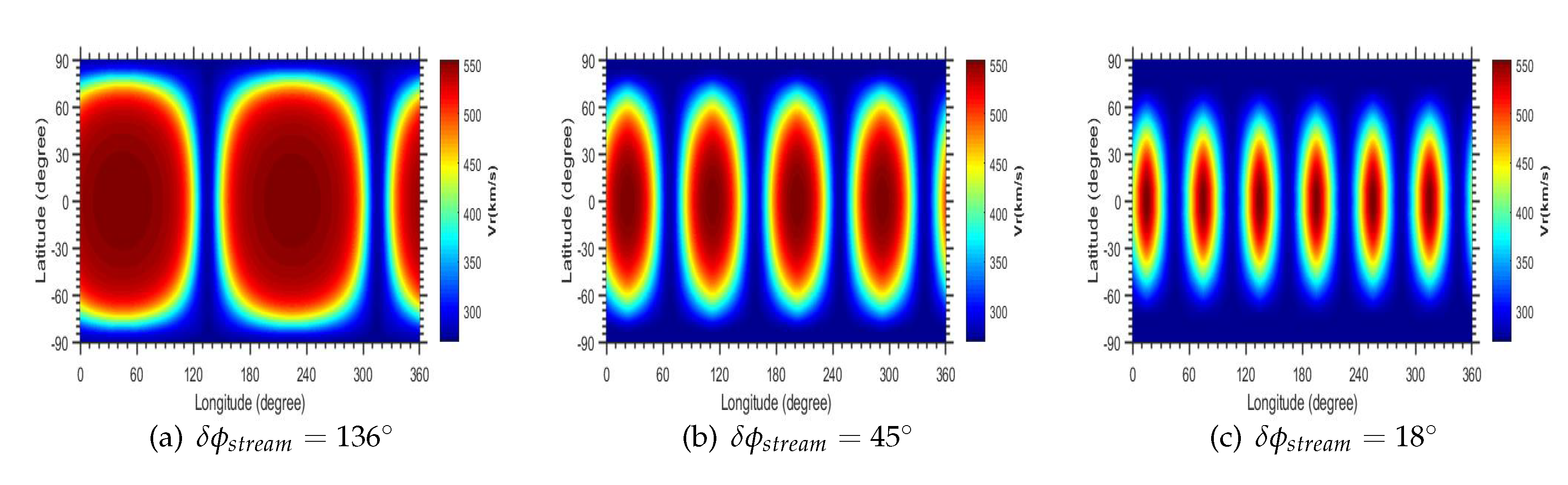
Figure 2.
The CIR width of the cases selected. The blue, red and yellow asterisks indicate the CIR radial extent, width projected into the solar equatorial plane and CIR width considering 3D geometry, respectively.
Figure 2.
The CIR width of the cases selected. The blue, red and yellow asterisks indicate the CIR radial extent, width projected into the solar equatorial plane and CIR width considering 3D geometry, respectively.
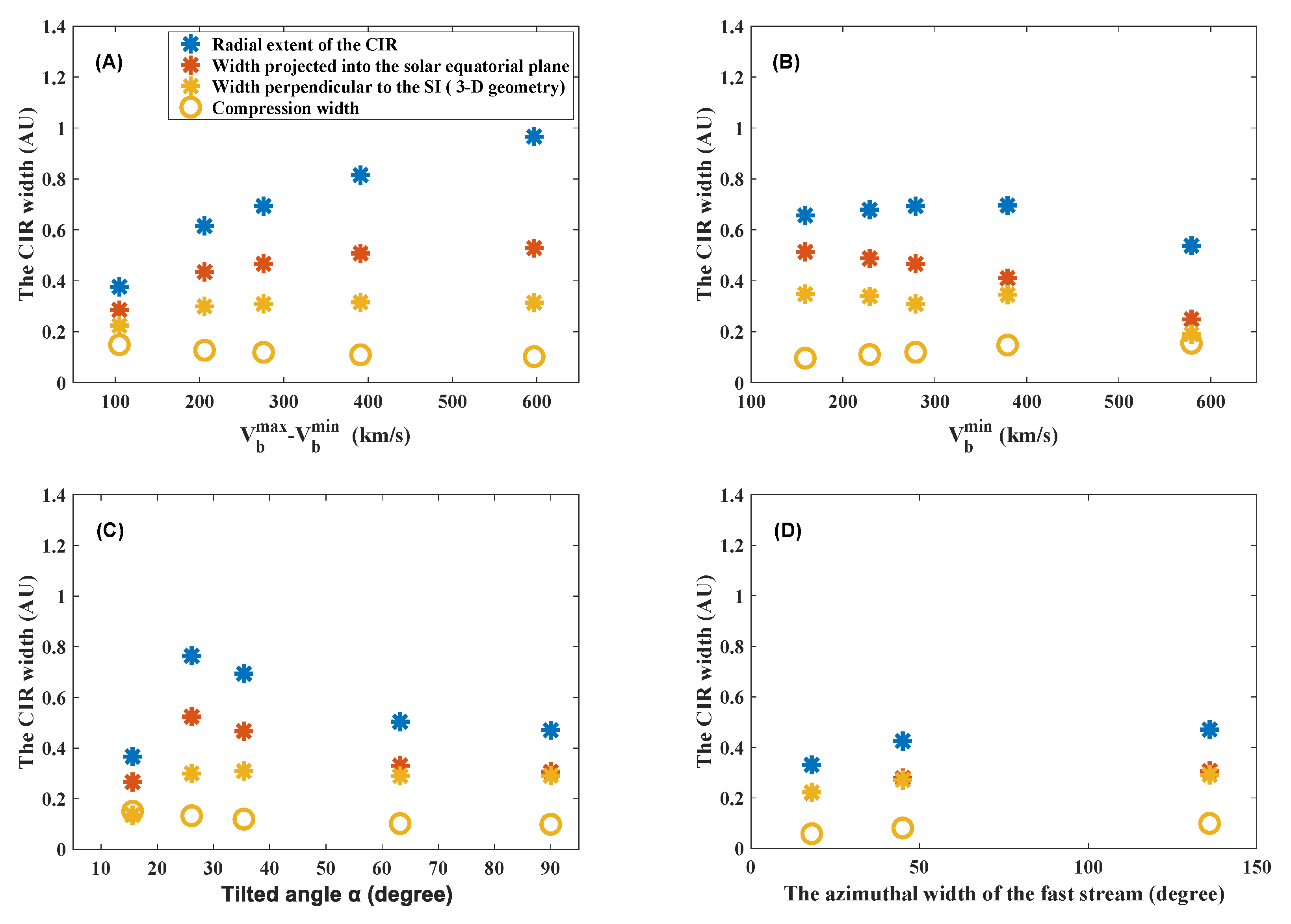
Figure 3.
The ratio of the maximum energy to the original energy () at 1AU after 60 hours versus the CIR parameters. The red and blue markers are for the reverse and the forward compression regions, respectively.
Figure 3.
The ratio of the maximum energy to the original energy () at 1AU after 60 hours versus the CIR parameters. The red and blue markers are for the reverse and the forward compression regions, respectively.
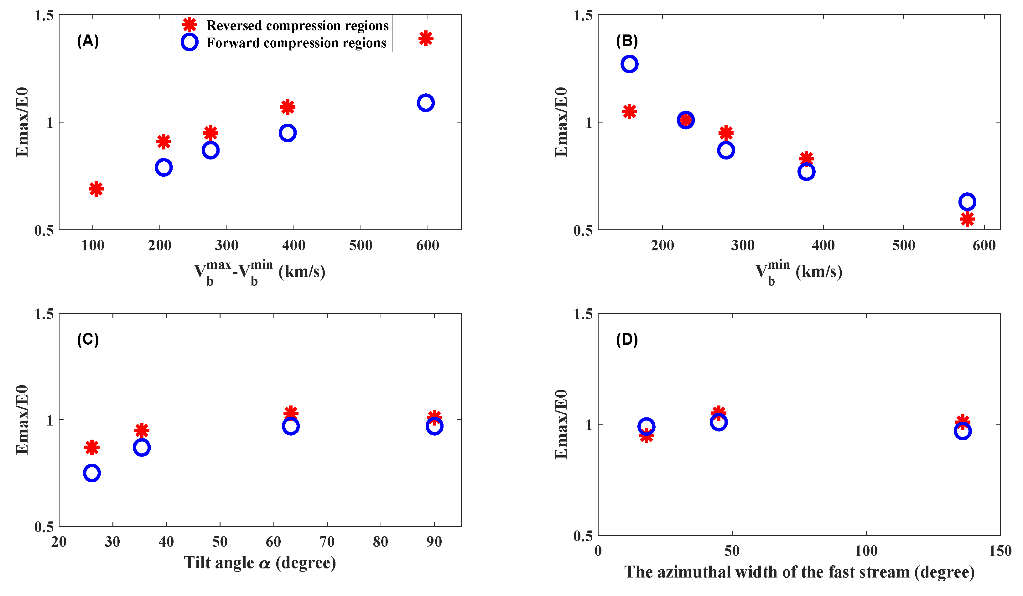
Figure 4.
The maximum ratio of the maximum energy in the reversed compression region to that in the approximated Parker region at 1 AU in the first 60 hours versus the CIR parameters. The blue asterisks, red circles, and yellow squares are for protons with original energy of 0.5 Mev, 5 MeV, and 20 MeV, respectively.
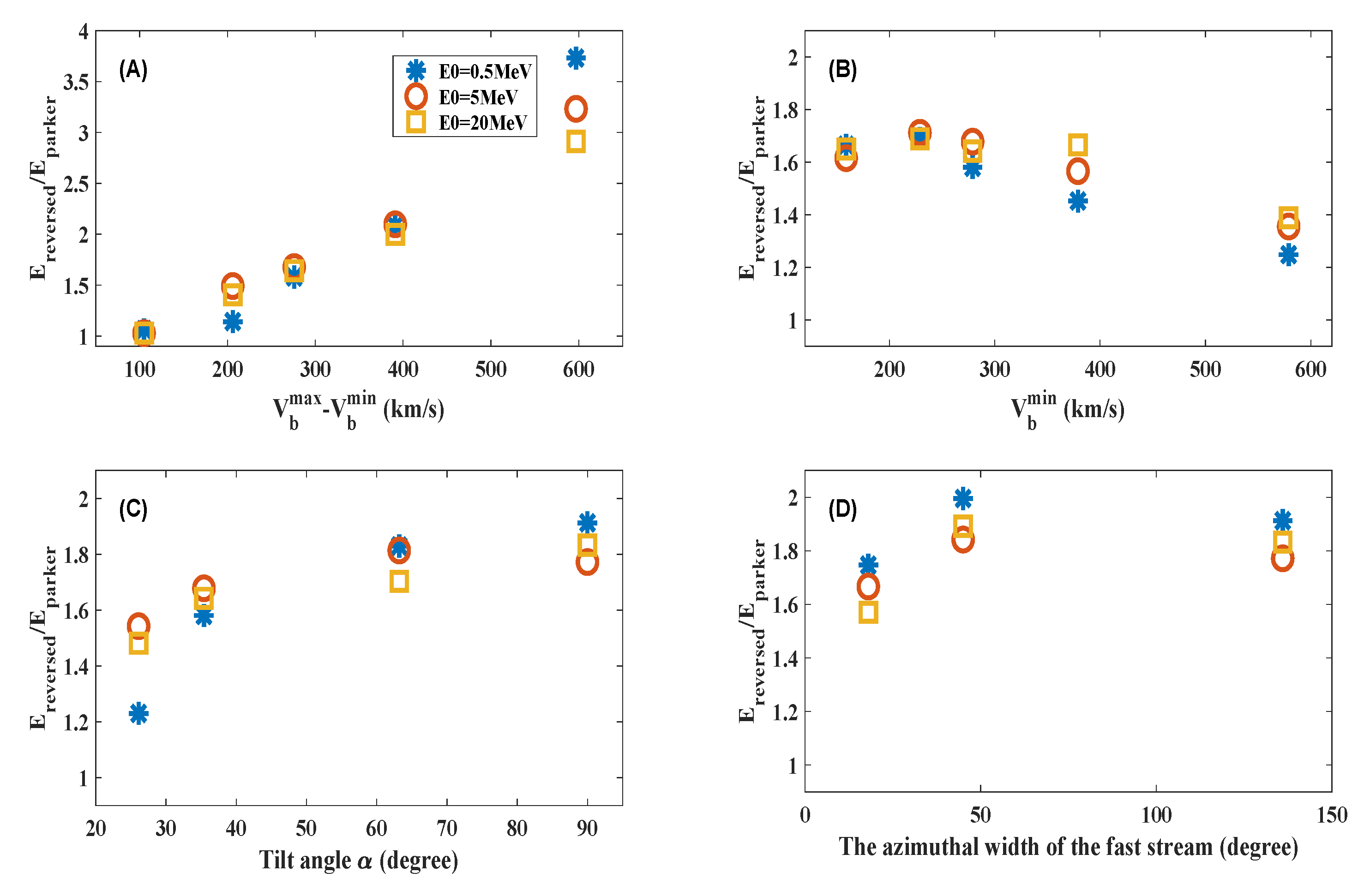
Figure 5.
The peak intensity versus the CIR width at 1 AU. The left panel shows peak intensity versus the compression width . The right panel shows peak intensity versus radial extent . The blue asterisks, red circles, yellow squares, and purple crosses indicate cases in Set A, Set B, Set C, and Set D, respectively.
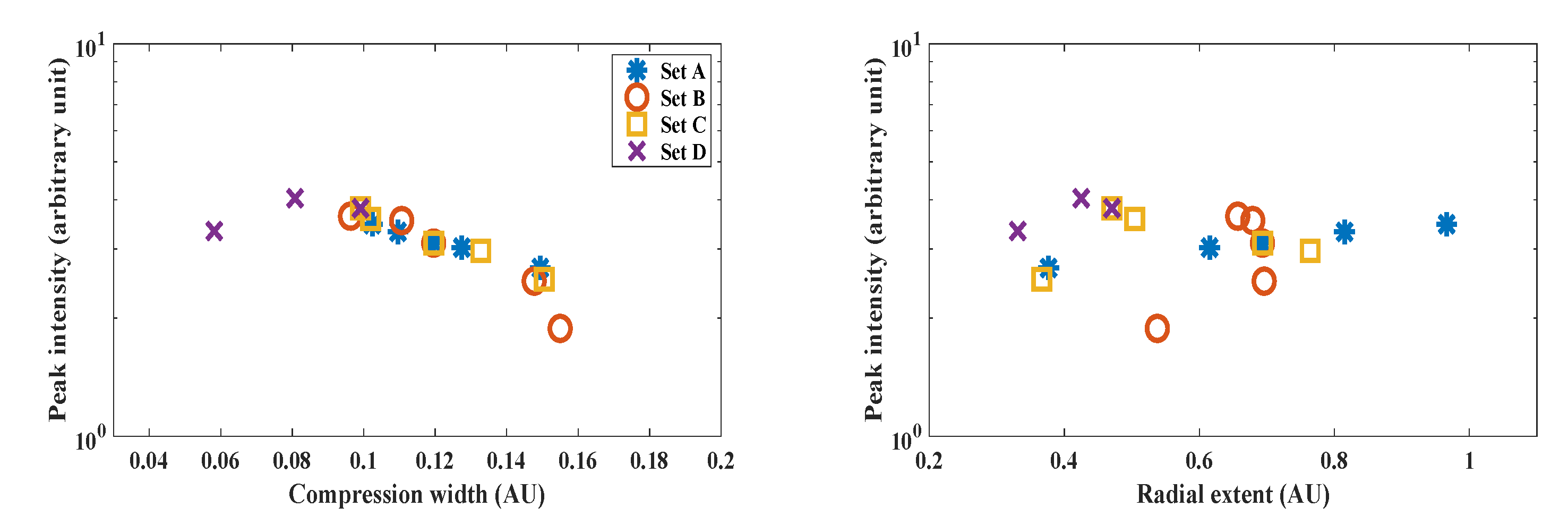
Figure 6.
The distribution of particle intensity with time, longitude, and radial distance for different cases. The rows from top to bottom display the cases in Set A, B, C, and D, respectively. The columns from left to right represent the distribution of particle intensity varying with time, longitude, and radial distance, respectively.
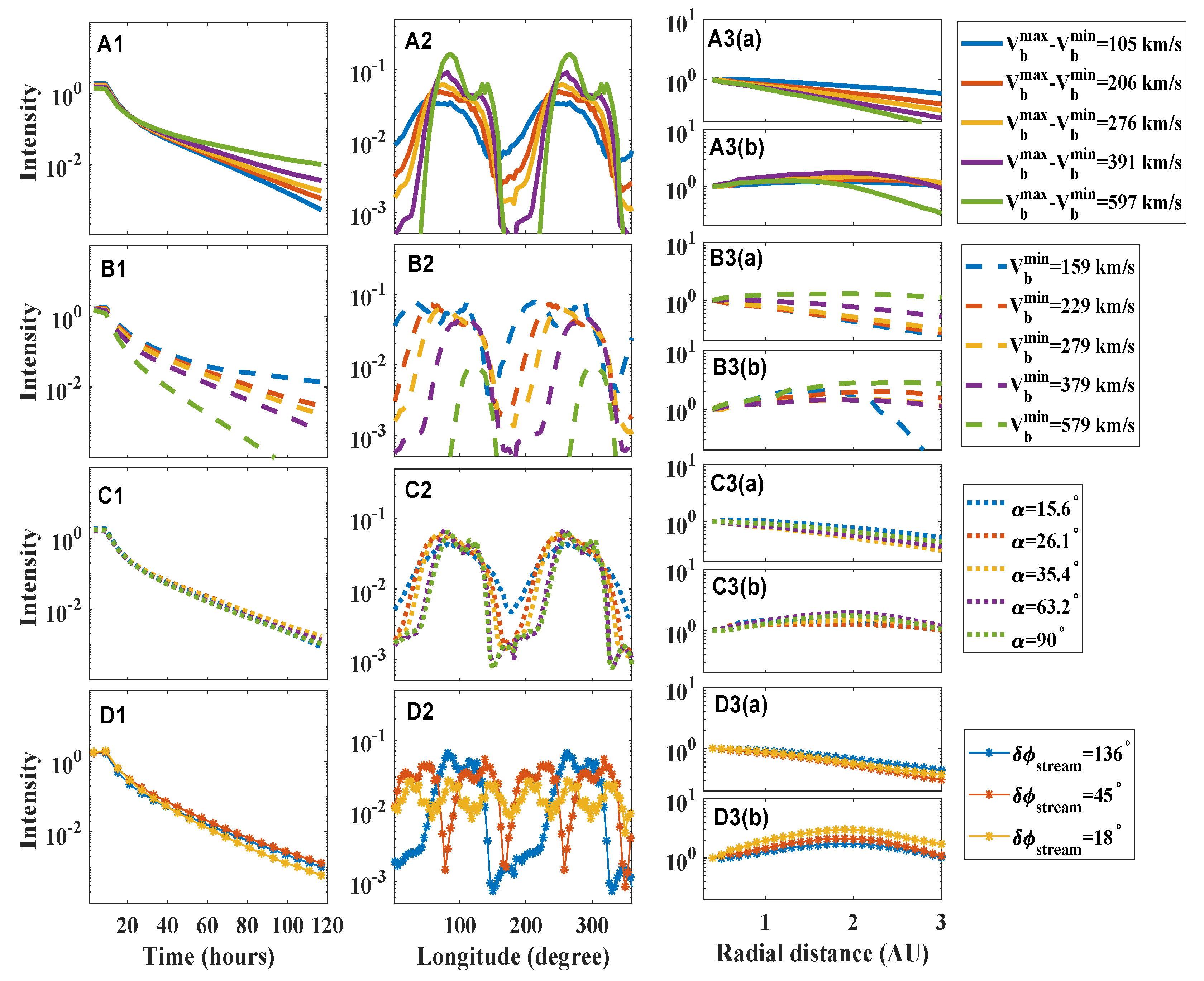

Table 1.
The parameters set in the backgrounds.
| Set A | Set B | Set C | Set D | |||||||||||||||
|---|---|---|---|---|---|---|---|---|---|---|---|---|---|---|---|---|---|---|
| Case Number | 1 | 2 | 3 | 4 | 5 | 1 | 2 | 3 | 4 | 5 | 1 | 2 | 3 | 4 | 5 | 1 | 2 | 3 |
| 35.4 | 35.4 | 15.6 | 26.1 | 35.4 | 63.2 | 90.0 | 90.0 | |||||||||||
| 279 | 579 | 379 | 279 | 229 | 159 | 279 | 279 | |||||||||||
| 384 | 485 | 555 | 670 | 876 | 855 | 655 | 555 | 505 | 435 | 555 | 555 | |||||||
| 105 | 206 | 276 | 391 | 597 | 276 | 276 | 276 | |||||||||||
| 1.4 | 1.7 | 2.0 | 2.4 | 3.1 | 1.5 | 1.7 | 2.0 | 2.2 | 2.7 | 2.0 | 2.0 | |||||||
| 306 | 309 | 309 | 313 | 318 | 673 | 433 | 309 | 246 | 158 | 309 | 309 | |||||||
| 434 | 556 | 640 | 778 | 1021 | 997 | 759 | 640 | 580 | 496 | 640 | 640 | |||||||
| 128 | 247 | 331 | 465 | 703 | 324 | 326 | 331 | 334 | 338 | 331 | 331 | |||||||
| ∖ | ∖ | ∖ | 136 | 45 | 18 | |||||||||||||
Disclaimer/Publisher’s Note: The statements, opinions and data contained in all publications are solely those of the individual author(s) and contributor(s) and not of MDPI and/or the editor(s). MDPI and/or the editor(s) disclaim responsibility for any injury to people or property resulting from any ideas, methods, instructions or products referred to in the content. |
© 2024 by the authors. Licensee MDPI, Basel, Switzerland. This article is an open access article distributed under the terms and conditions of the Creative Commons Attribution (CC BY) license (http://creativecommons.org/licenses/by/4.0/).
Copyright: This open access article is published under a Creative Commons CC BY 4.0 license, which permit the free download, distribution, and reuse, provided that the author and preprint are cited in any reuse.


