The Least Surprising Theory: An Information-Theoretic Approach to the Unification of Physics

1. Introduction

1.1. Physics from Inference

Given an amplitude $\psi$, a covariant exterior derivative $\mathbb{D}$ with curvature ${\mathbb{D}}^2$, and its Clifford contraction D, we form the displacement and reference jets

$$\begin{array}{cc}\hfill {\mathfrak{J}}_{ϵ}\psi :=\left(\psi +iϵD\psi ,\sqrt{ϵ}{\mathbb{D}}^2\right),& \hfill {\mathfrak{J}}_r\psi :=\left(\psi ,0\right).\end{array}$$

(1)

Their normalized complex comparison defines the complexified transition surprisal

$$\begin{array}{cc}\hfill \mathcal{K}\left({\mathfrak{J}}_{ϵ}\psi ,{\mathfrak{J}}_r\psi \right)& :=-ln{\displaystyle \frac{{〈{\mathfrak{J}}_r\psi |{\mathfrak{J}}_{ϵ}\psi 〉}_{\mathfrak{J}}}{\sqrt{{〈{\mathfrak{J}}_r\psi |{\mathfrak{J}}_r\psi 〉}_{\mathfrak{J}}{〈{\mathfrak{J}}_{ϵ}\psi |{\mathfrak{J}}_{ϵ}\psi 〉}_{\mathfrak{J}}}}}=-iϵ\left[Re\langle \psi \mid D\psi \rangle -{\displaystyle \frac{1}{2}}{∥{\mathbb{D}}^2∥}^2\right]+O\left({ϵ}^2\right)\hfill \end{array}$$

(2)

Accumulation retains its first-order coefficient:

$$\underset{ϵ\to 0}{lim}{\displaystyle \frac{1}{ϵ}}\mathcal{K}\left({\mathfrak{J}}_{ϵ}\psi ,{\mathfrak{J}}_r\psi \right)=-i{\int }_X{\mathrm{d}}^{d}x\sqrt{\left|g\right|}\left[Re{\langle \psi \mid D\psi \rangle }_x-{\displaystyle \frac{1}{4}}tr\left(F_{\mu \nu }{F}^{\mu \nu }\right)\right]$$

(3)

whose real coefficient is the action. Its stationary field configurations—the histories of least surprisal—satisfy the Dirac and Yang–Mills equations. Fundamental theory construction thus amounts to transition jets construction and then, to accumulate their surprisal.

Our main result introduces the spacetime transition jets, resulting in a unified matter-gravity action after surprisal accumulation. The wavefunction is parametrized by the pointwise metric bundle $(x,g_x)$ and the current stabilizer $u\in U\left(2\right)$. It takes value in:

$$\mathsf{\Psi }(x,g_x,u)\in {Cl}^{+}(T_{x}X,g_x)\otimes {\mathsf{\Sigma }}^{\epsilon }\left({Sym}^2\left(T_x^{*}X\right),G_{g_x}\right),\epsilon \in \{+,-\}.$$

(4)

where $G_{g_x}$ is the DeWitt form on metric variations. Unlike GUT constructions, here the structures always exist in spacetime. The fibre realizes a particle sector with ambient spin-frame symmetry $Spin(6,4)$ and a family sector which, under polarization, complex structure, and unimodularity assumptions, reduce to the three-generation Standard Model. Surprisal accumulation ${lim}_{ϵ\to 0}{\displaystyle \frac{1}{ϵ}}\mathcal{K}\left({\mathfrak{J}}_{ϵ}\mathsf{\Psi },{\mathfrak{J}}_r\mathsf{\Psi }\right)$ then furnishes the fermion kinetic and Yukawa terms, the Yang–Mills terms $F_{\mu \nu }{F}^{\mu \nu }$, the Higgs kinetic and quartic terms, the nonminimal coupling $R{H}^{†}H$ and the CKM and PMNS matrices together with the gravitational terms $\mathsf{\Lambda }$, R, $R^2$, and $C_{\mu \nu \rho \sigma }{C}^{\mu \nu \rho \sigma }$, yielding the three-generation Standard Model coupled to power-counting-renormalizable gravity. Finally, the opposite-norm massive spin-two sector of quadratic gravity is addressed by an intensity-positive measurement theory. Insofar as the jets describe spacetime transitions, the resulting action is the least-surprising theory native to spacetime.

Jaynes (1957) observed that statistical mechanics need not be derived from mechanics at all. Extremizing the Shannon entropy

$$S\left[p\right]=-\sum _i{p}_{i}ln{p}_i\mathrm{subject}\mathrm{to}\sum _i{p}_i{f}_k^{\left(i\right)}=\langle f_k\rangle$$

(5)

returns the Gibbs distribution,

$$p_i\propto exp\left(-\sum _k{\lambda }_k{f}_k^{\left(i\right)}\right),$$

(6)

the multipliers ${\lambda }_k$ being fixed by the constraints. No ergodic hypothesis is required and nothing is assumed about the underlying dynamics; thermodynamics on this reading is a rule of inference rather than a physical law.

The reframing was more ambitious than a rederivation. If one part of physics is inference under constraint, the rest may be as well, and the laws would then not be brute facts but the least biased account of nature available given what is held fixed. We shall call this the inferential programme. The present work is an attempt to complete it; the two subsections that follow set out what has been achieved within it and why it has not been completed before.

Paths.

Jaynes extended the construction from states to histories. In place of a distribution over configurations one seeks a distribution over trajectories, extremizing the path entropy—the caliber—subject to constraints on path functionals $F_k\left[x\right]$. The output has the same form as (6),

$$p\left[x\left(t\right)\right]\propto exp\left(-\sum _k{\lambda }_k{F}_k\left[x\right]\right),$$

(7)

from which follow diffusion, the fluctuation theorems and Onsager reciprocity; Pressé et al. (2013) survey the construction and its applications.

Updates.

A further refinement takes the object of inference to be not a distribution but the revision of one. Given a reference $\rho$, the least biased revision is measured by the relative entropy, and for nearby distributions

$$D\left(\rho +\delta \rho \parallel \rho \right)={\displaystyle \frac{1}{2}}\int {\displaystyle \frac{{\left(\delta \rho \right)}^2}{\rho }}+O\left(\delta {\rho }^3\right),$$

(8)

whose leading term is the Fisher–Rao metric.

Quantum mechanics.

That line reached a landmark in the recovery of the Schrödinger equation (Hall and Reginatto 2002; Reginatto 1998). A classical ensemble is described by a density $\rho$ and a Hamilton–Jacobi action S, with ensemble Hamiltonian

$${\mathcal{H}}_{\mathrm{cl}}[\rho ,S]=\int {\mathsf{d}}^{3}x\rho \left[{\displaystyle \frac{{|\nabla S|}^2}{2m}}+V\right],$$

(9)

whose stationary points are the continuity and Hamilton–Jacobi equations. Adding the Fisher information of the density,

$$\mathcal{H}[\rho ,S]={\mathcal{H}}_{\mathrm{cl}}[\rho ,S]+\lambda \int {\mathsf{d}}^{3}x{\displaystyle \frac{{|\nabla \rho |}^2}{\rho }},\lambda ={\displaystyle \frac{{\hslash }^2}{8m}},$$

(10)

and writing $\psi =\sqrt{\rho }{e}^{iS/\hslash }$, the two stationarity conditions become the real and imaginary parts of

$$i\hslash {\partial }_t\psi =\left(-{\displaystyle \frac{{\hslash }^2}{2m}}{\nabla }^2+V\right)\psi .$$

(11)

The Fisher term contributes exactly the quantum potential $-\frac{{\hslash }^2}{2m}{\nabla }^2\sqrt{\rho }/\sqrt{\rho }$; the remainder of (11) comes from (9). The Schrödinger equation as a statement about inference rather than a postulate about nature is a genuine success of the programme.

Everything else.

Frieden (1998) carried the idea furthest. In the principle of extreme physical information a measurement is a transfer of information from source to observer, and the equations of physics are the extrema of $I-J$, with I the Fisher information of the observed data and J the bound information of the source. With appropriate choices of J the principle returns the Klein–Gordon, Maxwell and Einstein equations and the Boltzmann distribution.

1.2. Why Each Fell Short

In the guise of completing the inference programme, the sequence above is a sequence of repairs, and each repair leaves something undone.

Maximum entropy assigns a distribution at an instant. It says nothing about evolution, and (6) contains no time. Maximum caliber answers this, replacing distributions over states by distributions over histories.

Maximum caliber therefore delivers dynamics, but (7) is real and positive, and real positive weights do not interfere. What it delivers is stochastic—diffusion and its relatives—and the passage to quantum dynamics still needs $\beta \to i\tau$; that is, it introduces complex amplitudes by fiat. Replacing the entropy by the Fisher information answers this: (11) is quantum, and no rotation was performed to obtain it.

The Fisher route at first appears promising but falls short for two reasons. The first is structural. A divergence vanishes and is stationary where its arguments agree, so (8) has no first-order term and its leading content is the quadratic form; such a principle can supply a metric and nothing else. A metric is a second-order kinetic term, and in (10) that is precisely what it is—the quantum potential, the term of order ${\hslash }^2$—while the kinetic and potential energies are imported with ${\mathcal{H}}_{\mathrm{cl}}$. Second order is moreover the wrong order for fundamental matter. The Dirac Lagrangian $\overline{\psi }i{\gamma }^{\mu }{\partial }_{\mu }\psi$ is linear in the derivative, and it is that linearity which carries the conserved current $\overline{\psi }{\gamma }^{\mu }\psi$ and its positive density; no functional stationary at coincidence produces a term linear in the displacement. Extreme physical information is no counterexample: its extremization returns the Klein–Gordon equation, second order as expected, and Dirac’s equation follows only on factorizing that output—the step Dirac (1928) took in 1928, performed to fix the landed result rather than derived from the principle.

The second reason is methodological. Streater (2007) observes that the bound information J is chosen so that the extremum of $I-J$ is the equation sought, and that as the target theory becomes more structured more of the content sits in J than in the informational term. The breadth of the principle’s reach is bought at the cost of its discriminating power. The result is a program that admits anything at second order, and nothing at first.

1.3. Surprisal

At minimum what is wanted, then, is an informational quantity whose expansion about identical arguments has a first-order term. There is one, and it is the oldest: the surprisal $-ln\rho$ of a single event.

Unlike entropy, surprisal requires no sum, and so needs no ensemble. The decisive step is to attach complexified transition surprisal to the normalized complex comparison of a displacement jet and a reference jet. Jets allow the surprisal of both the $\psi \to \psi +iϵD\psi$ and the $0\to \sqrt{ϵ}{\mathbb{D}}^2$ transitions to simultaneously contribute to the same action phase. The full construction is given in Definitions 1–3.

Where relative maximum entropy delivers the least biased revision given constraints, transition surprisal delivers the least surprising update given a displacement from a reference. The two stand in the same relation to their inputs.

$$\begin{array}{c}\hfill \underset{\mathbf{The}\mathbf{least}\mathbf{biased}\mathbf{revision}}{\underbrace{D\left(\rho +\delta \rho \parallel \rho \right)=\frac{1}{2}\int {\displaystyle \frac{{\left(\delta \rho \right)}^2}{\rho }}+\dots }}\mathrm{vs}.\underset{\mathbf{The}\mathbf{least}\mathbf{surprising}\mathbf{update}}{\underbrace{\mathcal{K}\left({\mathfrak{J}}_{ϵ}\psi ,{\mathfrak{J}}_r\psi \right)=-iϵ\left[\langle \psi \mid D\psi \rangle +{\displaystyle \frac{s_F}{2}}{∥{\mathbb{D}}^2-{\mathbb{F}}_0∥}^2\right]+\dots }}.\end{array}$$

(12)

Both quantities measure the informational cost of a change relative to a reference. Relative entropy is real and begins at second order. The state displacement in the jet comparison has a first-order term, which is imaginary and oriented: it changes sign when the displacement is reversed, as a divergence between probability distributions cannot. The curvature comparison is intrinsically quadratic, but its $\sqrt{ϵ}$ scaling makes it contribute at the same accumulated order, while the signature-dependent complex jet pairing places it in the same action phase. Nothing need be imported alongside them: kinetic terms, potentials and curvature terms arise from the transport, reference and invariant pairings of the jets during surprisal accumulation, so there is no analogue of a supplementary source J chosen to reproduce a predetermined equation.

The resulting expression is precisely the global form required of an action. A field history with real action S has the one-parameter transition weight

$${\mathcal{A}}_{ϵ}=e^{iϵS},$$

(13)

where $ϵ$ is the dimensionless deformation parameter of the jets. Its transition surprisal, on the continuous local logarithm branch at $ϵ=0$, is

$$-ln{\mathcal{A}}_{ϵ}=-ln{e}^{iϵS}=-iϵS.$$

(14)

With the carrier pairings understood as global $L^2$ pairings, comparison with (12) therefore identifies

$$\begin{array}{cc}\hfill S& =Re\langle \psi \mid D\psi \rangle +{\displaystyle \frac{s_F}{2}}{∥{\mathbb{D}}^2-{\mathbb{F}}_0∥}^2\hfill \\ \hfill & ={\int }_X{\mathsf{d}}^{d}x\sqrt{\left|g\right|}\left[Re{\langle \psi \mid D\psi \rangle }_x+{\displaystyle \frac{s_F}{2}}{∥{\mathbb{D}}^2-{\mathbb{F}}_0∥}_x^2\right].\hfill \end{array}$$

(15)

The expression in brackets is the local Lagrangian density,

$$\mathcal{L}=Re{\langle \psi \mid D\psi \rangle }_x+{\displaystyle \frac{s_F}{2}}{∥{\mathbb{D}}^2-{\mathbb{F}}_0∥}_x^2,S={\int }_X{\mathsf{d}}^{d}x\sqrt{\left|g\right|}\mathcal{L}.$$

(16)

The least-surprising update thus has exactly the form of the surprisal of an action amplitude. Accumulation extracts the first-order coefficient of the jet comparison and gives

$$\mathcal{I}=\underset{ϵ\to 0}{lim}{\displaystyle \frac{{\mathcal{K}}_{ϵ}}{ϵ}}=-iS,e^{-\mathcal{I}}=e^{iS}.$$

(17)

Our claim is accordingly that the inferential programme was right but the functionals considered were wrong. Not entropy, relative entropy or Fisher information, but the surprisal of the transition between a displacement jet and a reference jet. In other words, the universe does not evolve according to the least biased revision; it evolves according to the least surprising update.

1.4. The Ansatz

Ordinarily, a carrier is chosen to realize a Lagrangian already given: the theory determines which fields, representations, and internal spaces must be supplied. Accumulated surprisal permits the reverse direction. Given a carrier and its transition jets, surprisal accumulates to the action. Thus, fundamental theory construction is reducible to transition jets construction.

This simplifies theory construction sufficiently that a power-counting-renormalizable unified matter-gravity theory can be attempted by Ansatz. This constitutes our main result.

To that end, we introduce the spacetime transition jets. We begin with their carrier, whose amplitude and parameter spaces are constructed exclusively from structures that spacetime itself supplies. The jets then describe transitions over these structures, and its surprisal accumulates to the action. Specifically, we use the following spacetime structures:

(i)

The pair $(x,g_x)$ supplies the even spacetime algebra

$${Cl}^{+}(T_{x}X,g_x),$$

(18)

which realizes the Dirac amplitude in the Dirac–Hestenes formulation of spacetime algebra.

(ii)

Retaining the local metric $g_x$ as a parameter supplies the tangent space to the pointwise metric fibre,

$$V_{x,g}:=T_{g_x}{\mathcal{M}}_{1,3,x}\left(X\right)\cong {Sym}^2\left(T_x^{*}X\right),$$

(19)

together with its DeWitt form $G_{g_x}$ and an irreducible chiral spin carrier

$${\mathsf{\Sigma }}^{\epsilon }(V_{x,g},G_{g_x}),\epsilon \in \{+,-\}.$$

(20)

(iii)

The even spacetime algebra satisfies

$${Cl}^{+}(1,3)\cong {Mat}_2\left(\mathbb{C}\right)$$

(21)

as a real algebra. Its left $Spin(1,3)$ action commutes with a nongauged right action. The right transformations preserving the Dirac current

$$J\left(\psi \right)=\psi {\gamma }_0\tilde{\psi }$$

(22)

satisfy

$$J\left(\psi U\right)=\psi U{\gamma }_0\tilde{U}\tilde{\psi }=J\left(\psi \right),U{\gamma }_0\tilde{U}={\gamma }_0,$$

(23)

and form the internal group

$$U{\left(2\right)}_{\mathrm{fam}}\cong {\displaystyle \frac{SU\left(2\right)\times U\left(1\right)}{{\mathbb{Z}}_2}}.$$

(24)

Because this group acts from the right, it commutes with the left spacetime-spin action and cannot be reached by a Lorentz transformation. We retain its coordinate $u\in U{\left(2\right)}_{\mathrm{fam}}$ as a nongauged family parameter.

We therefore make the Ansatz

$$\mathsf{\Psi }=\mathsf{\Psi }(x,g_x,u),u\in U{\left(2\right)}_{\mathrm{fam}},$$

(25)

with pointwise values

$$\mathsf{\Psi }(x,g_x,u)\in {Cl}^{+}(T_{x}X,g_x)\otimes {\mathsf{\Sigma }}^{\epsilon }\left({Sym}^2\left(T_x^{*}X\right),G_{g_x}\right),\epsilon \in \{+,-\}.$$

(26)

Unlike conventional GUT constructions, the carrier structures used here are not hypothetical internal spaces: they are supplied by the spacetime algebra and the geometry of local metric variations, and therefore exist pointwise wherever the selected spacetime arena exists. The construction is therefore more economical (and importantly more restrictive) that GUT constructions. Although the present construction remains an Ansatz, it introduces only the limited choices required to select a physical realization of these spacetime-native structures. As shown below, those choices are retrodictively vindicated by the unified matter–gravity theory on which their accumulated surprisal closes.

Using this carrier, a general spacetime transition is represented by the jets

$$\begin{array}{cc}{\mathfrak{J}}_{ϵ}\mathsf{\Psi }:=\left(\mathsf{\Psi }+iϵD_{\mathrm{ST}}\mathsf{\Psi },\sqrt{ϵ}{\mathbb{D}}_{\mathrm{ST}}^2\right),\hfill & {\mathfrak{J}}_r\mathsf{\Psi }:=\left(\mathsf{\Psi },\sqrt{ϵ}{\mathbb{F}}_{0,\mathrm{ST}}\right).\hfill \end{array}$$

(27)

Here ${\mathbb{D}}_{\mathrm{ST}}$ is a covariant transport on the native carrier, $D_{\mathrm{ST}}$ is its contracted first-order operator, and ${\mathbb{D}}_{\mathrm{ST}}^2$ is its curvature. The reference ${\mathbb{F}}_{0,\mathrm{ST}}$ specifies the curvature and vacuum configuration declared unsurprising. The subscript $\mathrm{ST}$ indicates that the transport acts on the complete spacetime carrier, including its spacetime, metric-fibre, and family dependence.

Applying transition surprisal to (27) gives

$$\mathcal{K}\left({\mathfrak{J}}_{ϵ}\mathsf{\Psi },{\mathfrak{J}}_r\mathsf{\Psi }\right)=-iϵ\left[Re〈\mathsf{\Psi }|D_{\mathrm{ST}}\mathsf{\Psi }〉+{\displaystyle \frac{s_F}{2}}{∥{\mathbb{D}}_{\mathrm{ST}}^2-{\mathbb{F}}_{0,\mathrm{ST}}∥}^2\right]+O\left({ϵ}^2\right).$$

(28)

Their accumulated surprisal therefore determines the action

$$\begin{array}{c}{\mathcal{I}}_{\mathrm{ST}}:=\underset{ϵ\to 0}{lim}{\displaystyle \frac{1}{ϵ}}\mathcal{K}\left({\mathfrak{J}}_{ϵ}\mathsf{\Psi },{\mathfrak{J}}_r\mathsf{\Psi }\right)=-i{S}_{\mathrm{ST}},\hfill \\ S_{\mathrm{ST}}={\int }_X{\mathsf{d}}^{4}x\sqrt{-g}\left[Re{〈\mathsf{\Psi }|D_{\mathrm{ST}}\mathsf{\Psi }〉}_{\mathrm{fib}}+{\displaystyle \frac{s_F}{2}}{∥{\mathbb{D}}_{\mathrm{ST}}^2-{\mathbb{F}}_{0,\mathrm{ST}}∥}_{\mathrm{fib}}^2\right],\hfill \end{array}$$

(29)

where the fibre pairing includes the metric-fibre and family dependence retained by the carrier. The explicit transport, its curvature decomposition, the reference, and the corresponding fibre pairings are assembled in Section 3.5.

As shown in Section 3.3, the metric-variation space has signature $(6,4)$ and ambient spin-frame symmetry $Spin(6,4)$. Positive definiteness of the particle density selects a positive polarization $R_x$ and restricts maximal compatible transport to the Pati–Salam group. A compatible complex structure $J_x$ and unimodularity then select the faithful Standard Model realization:

$$\begin{array}{|c|}\hline Spin(6,4)\stackrel{R_x}{\to }{G}_{\mathrm{PS}}\stackrel{J_x}{\to }U\left(3\right)\times U\left(2\right)\stackrel{\mathrm{unimodularity}}{\to }{G}_{\mathrm{SM}}.\\ \hline\end{array}$$

(30)

Independently, in Section 3.4, we show that the reduction of the nongauged family structure gives

$$U{\left(2\right)}_{\mathrm{fam}}⟶U\left(1\right)\times U\left(1\right),{\displaystyle \frac{U{\left(2\right)}_{\mathrm{fam}}}{U\left(1\right)\times U\left(1\right)}}\cong {\mathbb{CP}}^1.$$

(31)

Its tangent-equivariant sector is

$$T^{1,0}{\mathbb{CP}}^1\cong \mathcal{O}\left(2\right),$$

(32)

and the corresponding Dolbeault–Dirac operator has index three. The metric-fibre half-spin module therefore supplies the particle content of one generation, while the STA family sector supplies three chiral copies.

Finally, in Section 3.6, we obtain the zero-mode sector of the resulting action and show that it is the three-generation Standard Model coupled to quadratic gravity, which is local and power-counting renormalizable:

$$\begin{array}{cc}\hfill S_{\mathrm{SM}+\mathrm{QG}}^{\left(3\right)}& ={\int }_X{\mathsf{d}}^{4}x\sqrt{-g}[a{C}_{\mu \nu \rho \sigma }{C}^{\mu \nu \rho \sigma }+b{R}^2+c{E}_4+{\displaystyle \frac{M_{\mathrm{P}}^2}{2}}R-\mathsf{\Lambda }\hfill \\ \hfill & -{\displaystyle \frac{1}{4g_3^2}}{G}_{\mu \nu }^A{G}^{A\mu \nu }-{\displaystyle \frac{1}{4g_2^2}}{W}_{\mu \nu }^I{W}^{I\mu \nu }-{\displaystyle \frac{1}{4g_1^2}}{B}_{\mu \nu }{B}^{\mu \nu }\hfill \\ \hfill & +{\displaystyle \sum _{n=1}^3}\sum _f{\overline{\psi }}_{f,n}i{\gamma }^{\mu }{D}_{\mu }^{\mathrm{SM}}{\psi }_{f,n}-{\left(D_{\mu }^{\mathrm{SM}}H\right)}^{†}{D}^{\mu ,\mathrm{SM}}H-\xi R{H}^{†}H\hfill \\ \hfill & -m_H^2{H}^{†}H-{\lambda }_H{\left(H^{†}H\right)}^2\hfill \\ \hfill & -\left({\overline{Q}}_L{Y}_u\tilde{H}{u}_R+{\overline{Q}}_L{Y}_{d}H{d}_R+{\overline{L}}_L{Y}_{e}H{e}_R+{\overline{L}}_L{Y}_{\nu }\tilde{H}{\nu }_R+\mathrm{h}.\mathrm{c}.\right)\hfill \\ \hfill & -{\displaystyle \frac{1}{2}}\left(\overline{{\nu }_R^c}{M}_R{\nu }_R+\mathrm{h}.\mathrm{c}.\right)],\hfill \end{array}$$

(33)

where $\tilde{H}=i{\sigma }_2{H}^{*}$, and the Yukawa and Majorana couplings are matrices on the three-dimensional family zero-mode space. The complete action is accumulated over spacetime and the family orbit and additionally contains the nonzero family-excitation spectrum.

This subsection states the destination of the construction. The arena, native carrier, particle and family reductions, three-generation spectrum, and operator sectors entering (33) are developed in Section 3.

1.5. An Observer Internal to the Universe

Accumulated surprisal produces an action quadratic in the curvature. For a gauge connection this is precisely the Yang–Mills term, and its quantization is unproblematic. The spin connection enjoys no such protection: the Riemann curvature already contains two derivatives of the metric, so its square is a four-derivative action—quadratic gravity, containing $C_{\mu \nu \rho \sigma }{C}^{\mu \nu \rho \sigma }$ and $R^2$ alongside the Einstein–Hilbert term R and the cosmological term $\mathsf{\Lambda }$. Since the procedure cannot avoid this outcome, the standing objections to quadratic gravity must be addressed lest the theory be discarded. There are two. The dynamical objection—stability—is taken up in Section 1.6. The kinematical objection, addressed here, is that retaining the massive opposite-norm spin-two mode (Stelle, 1977) places the state space in a Krein space rather than a Hilbert space: the kinematical carrier of (33) is the Hilbert–Krein space

$$K_{universe}={\mathcal{H}}_{\mathrm{SM}}^{\left(3\right)}\widehat{\otimes }{K}_{\mathrm{QG}},{\eta }_{universe}={\mathbb{1}}_{\mathrm{SM}}^{\left(3\right)}\otimes {\eta }_{\mathrm{QG}}.$$

(34)

A Krein space K carries a positive Hilbert topology $(·,·)$ together with a self-adjoint involution

$${\eta }^{†}=\eta ,{\eta }^2=\mathbb{1},$$

(35)

which defines the conserved indefinite form

$$[\varphi ,\psi ]:=(\varphi ,\eta \psi ).$$

(36)

The decomposition

$$K=K_{+}\oplus K_{-}{,\eta |}_{K_{\pm }}=\pm \mathbb{1},$$

(37)

admits nonzero states of positive, negative, or vanishing signed norm. Consequently, the conserved form cannot provide a universal positive normalization

$$[\psi ,\psi ]=1$$

(38)

for all physical states. If quantum measurement is assumed to require such a positively normalized state, the opposite-norm sector appears to have no measurement interpretation. This is the conventional negative-norm objection.

The objection mistakes the cure for the disease.

First, why it’s not a disease.

The objection conflates physical measurement with representation by a positively normalized probability measure. However, a detector need only return nonnegative, countably additive intensities, thus satisfying two of the three Kolmogorov axioms. Let

$$P_{\pm }={\displaystyle \frac{1}{2}}(\mathbb{1}\pm \eta ),A_{\pm }=\eta P_{\pm }.$$

(39)

Both channels are intensity-positive, since

$$I_{\pm }\left(\psi \right):=[\psi ,A_{\pm }\psi ]=(\psi ,P_{\pm }\psi )\ge 0.$$

(40)

Their sum gives the total positive intensity,

$$I_{+}\left(\psi \right)+I_{-}\left(\psi \right)=(\psi ,\psi ),$$

(41)

whereas their difference reconstructs the conserved signed Krein charge,

$$I_{+}\left(\psi \right)-I_{-}\left(\psi \right)=[\psi ,\psi ].$$

(42)

A negative conserved value is therefore not a negative detector event: it is a difference between two nonnegative detector records.

Intensities are standard in quantum optics, hence the present structure is already familiar. In balanced photodetection, the two photodetectors return nonnegative photon-count intensities, while their difference defines a signed photocurrent from which field quadratures are reconstructed. A negative quadrature or difference current is not a negative photon count; it records which positive channel has the greater intensity. Likewise, a signed Krein observable is reconstructed from differences of nonnegative intensities rather than measured as a negative event.

More generally, for a Krein-self-adjoint channel A,

$$I_A\left(\psi \right):=[\psi ,A\psi ]=(\psi ,\eta A\psi )$$

(43)

is nonnegative precisely when $\eta A\ge 0$. The order isomorphism

$$A⟼E:=\eta A$$

(44)

therefore identifies intensity-positive Krein channels with ordinary positive Hilbert-space effects. Since the intensity cone generates the full observable space, differences of nonnegative records recover signed observables and provide complete tomography. Section 4 develops this construction in full.

Second, why it is a cure.

An observer without a conserved global normalizer cannot prove that a quantum system has been exhaustively measured. We qualify such an observer as internal. By contrast, an external observer can. Internal observers are naturally suited to quantum cosmology because they resolve its longest standing philosophical objection: the need for an observer external to the universe. Intensities are precisely the records available to an internal observer. Such an observer accesses a finite, nonexhaustive collection of local channels, not every possible outcome of the system as a whole. The carrier

$$K_{universe}={\mathcal{H}}_{\mathrm{SM}}^{\left(3\right)}\widehat{\otimes }{K}_{\mathrm{QG}}$$

(45)

positions the observer externally to the particle physics sector (i.e., ${\mathcal{H}}_{\mathrm{SM}}^{\left(3\right)}$ is a Hilbert space) while internally to the universe (i.e., $K_{QG}$ and by extension $K_{universe}$ are Krein spaces).

The Krein structure is therefore not a defect of the quantum theory. Krein spaces are to internal observers, what Hilbert spaces are to external observers.

1.6. The Stability Objection

The second objection to quadratic gravity concerns its dynamics rather than its kinematics. A Krein-self-adjoint Hamiltonian,

$$H^{♯}=H,$$

(46)

generates Krein-unitary evolution, but its spectrum is constrained only to be symmetric under complex conjugation: nonreal eigenvalues occur in conjugate pairs $E,\overline{E}$, and their eigenvectors are necessarily null, $[\psi ,\psi ]=0.$ On such pairs, the total intensity may grow without bound,

$$I_{+}\left({\psi }_t\right)+I_{-}\left({\psi }_t\right)=({\psi }_t,{\psi }_t)⟶\infty ,$$

(47)

while $[{\psi }_t,{\psi }_t]$ remains exactly conserved. By contrast, intensities in Hilbert spaces are outright conserved, so this cannot happen. As Krein spaces provide no such innate guarantees, intensity boundedness is entirely determined by the dynamics of the theory. Specifically in quadratic gravity, the massive spin-two mode couples universally to the stress tensor, and interactions generically displace its pole into a complex-conjugate pair. This is the conventional stability objection.

The response of the literature has been to seek a unitary sector: a decomposition of the Krein space into a subspace of real spectrum and positive norm, dynamically preserved by the interactions, never populated from ordinary matter, and excisable in a Lorentz-invariant manner—completed by the assumption that the initial conditions of the universe lie within it. Each clause of this program remains unproven, its treatments of the complex-pair sector remain in explicit disagreement (Donoghue and Menezes, 2019; Kubo and Kugo, 2024), and the program as a whole is now in its sixth decade (Cutkosky et al., 1969; Lee and Wick, 1969).

The program, however, pursues two goals at once, and it is worth separating them. The first is a measurement theory: a preserved positive-definite subspace is a carrier on which the Born rule can be declared, and without one the theory appeared to have no measurement interpretation at all. The second is bounded dynamics: within such a sector, evolution is genuinely unitary and nothing grows. The first goal is discharged by the preceding subsection. Intensities furnish a measurement theory on the full Krein carrier directly—no protected subspace is required for detector records to be nonnegative, additive, and tomographically complete. What survives of the second goal is correspondingly weaker. With the measurement burden carried by intensities, the sector may remain krein-unitary: it suffices that the leak into the opposite-norm sector remain bounded. This is the equivalent program under a lesser constraint: intensity-boundedness of the Krein-unitary theory rather than reduction to a unitarity sector.

The evidence for boundedness is as follows. Classically, quadratic gravity exhibits no runaways below computable energy thresholds (Salvio, 2019). For the quantum theory, the operator analysis of the complex-ghost sector shows the corresponding structural property: ghost pairs are produced from ordinary matter only above a definite energy threshold, and the populated sector is anti-unstable—conjugate pairs carry real total energy and persist without amplification (Kubo and Kugo, 2024). Under a unitarity requirement this production is fatal, and it is on this ground that the operator analysis rejects the theory. Under intensity measurements it is a bounded transfer between signed channels— precisely what the framework tolerates. The dynamics is stable, in that no intensity diverges; the positive sector is metastable, in that its contents transfer into the opposite-norm reservoir. The first is what intensity-boundedness requires; the second is what it permits. We adopt this as a hypothesis supported where the dynamics has been solved exactly and denied nowhere; its residual conditions—the extension of anti-instability to the multi-ghost sector and the frame consistency of the complex-pair kinematics—are open questions within the operator formalism (Kubo and Kugo, 2024). The stability objection is thus not an axiomatic violation but an unfinished boundedness question, and every sector in which the dynamics has been solved answers it in the affirmative.

1.7. Conventions and Definitions

Throughout, $\hslash =1$. Unless stated otherwise, the signature is $(-,+,+,+)$, and the state pairing $\langle ·\mid ·\rangle$ is antilinear in its first argument.

To construct a Lagrangian from surprisal, we require a local complex comparison between a displaced amplitude and a reference. The parametrization of the amplitude supplies two forms of local data: its first-order transport and the curvature of that transport. We collect these data into jets and define transition surprisal directly from their normalized complex comparison.

Two operators built from the same connection must therefore be distinguished. The covariant exterior derivative $\mathbb{D}$ has curvature ${\mathbb{D}}^2$, while its contraction D is a first-order operator on the carrier, typically Clifford. They are not independent: D and ${\mathbb{D}}^2$ are respectively the contracted transport and curvature supplied by the same connection.

Definition 1 

(Jets). Let $\psi \in \mathcal{H}$, let $\mathbb{D}$ be a covariant transport with curvature ${\mathbb{D}}^2$ and contraction D, let $ϵ>0$, and let ${\mathbb{F}}_0$ be a curvature-valued reference. The displacement and reference jets of ψ are

$$\begin{array}{cccc}\hfill {\mathfrak{J}}_{ϵ}\psi & :=\left(\psi +iϵD\psi ,\sqrt{ϵ}{\mathbb{D}}^2\right),\hfill & \hfill {\mathfrak{J}}_r\psi & :=\left(\psi ,\sqrt{ϵ}{\mathbb{F}}_0\right),\hfill \end{array}$$

(48)

the first slot of the displacement jet being the infinitesimal unitary transport generated by D, and the reference jet supplying the state against which the displaced jet is compared.

Definition 2 

(Complex jet pairing). For $U=(u_1,u_2)$ and $V=(v_1,v_2)$ in the jet carrier ${\mathcal{H}}_{\mathfrak{J}}=\mathcal{H}\oplus {\mathcal{H}}_F$, define the complex jet pairing

$${\langle U\mid V\rangle }_{\mathfrak{J}}:=w_1\langle u_1\mid v_1\rangle +w_2\langle u_2\mid v_2\rangle ,{\displaystyle \frac{w_2}{w_1}}=-i{s}_F,s_F=\left\{\begin{array}{cc}-1\hfill & \mathit{Lorentzian},\hfill \\ +1\hfill & \mathit{Euclidean},\hfill \end{array}\right.$$

(49)

the slots being mutually orthogonal. Because their relative weight is imaginary, the resulting jet pairing is generally a complex comparison form rather than a Hermitian inner product. The form of the complex jet pairing places the surprisal of both arguments of the jets into the same action phase.

Definition 3 

(Transition surprisal). Let $U,V\in {\mathcal{H}}_{\mathfrak{J}}$ be jets for which the following comparison is nonzero and continuously connected to coincidence. The transition surprisal from V to U is the negative local logarithm of their normalized complex jet comparison,

$$\mathcal{K}(U,V):=-ln{\displaystyle \frac{{\langle V\mid U\rangle }_{\mathfrak{J}}}{\sqrt{{\langle V\mid V\rangle }_{\mathfrak{J}}{\langle U\mid U\rangle }_{\mathfrak{J}}}}},$$

(50)

where the square root and logarithm are chosen by continuous local continuation from coincidence, with $\mathcal{K}(V,V)=0$.

Proposition 1 

(Expansion of the jet surprisal). Let the jets be those of Definition 1, with normalized amplitude $\langle \psi \mid \psi \rangle =1$, and let the relative curvature-slot weight be

$$\sigma =-i{s}_F,s_F\in \{+1,-1\}.$$

(51)

If D is formally Hermitian and the curvature pairing is real and symmetric, then

$$\mathcal{K}\left({\mathfrak{J}}_{ϵ}\psi ,{\mathfrak{J}}_r\psi \right)=-iϵ\left[\langle \psi \mid D\psi \rangle +{\displaystyle \frac{s_F}{2}}{∥{\mathbb{D}}^2-{\mathbb{F}}_0∥}^2\right]+O\left({ϵ}^2\right),$$

(52)

and the coefficient in brackets is real.

Proof. 

Write

$$\begin{array}{cc}a:=\langle \psi \mid D\psi \rangle \in \mathbb{R},\hfill & b:={\parallel D\psi \parallel }^2,\hfill \end{array}$$

(53)

$$\begin{array}{ccc}c:=〈{\mathbb{F}}_0|{\mathbb{D}}^2〉\in \mathbb{R},\hfill & d:={\parallel {\mathbb{D}}^2\parallel }^2,\hfill & f:={\parallel {\mathbb{F}}_0\parallel }^2.\hfill \end{array}$$

(54)

The three pairings entering the normalized jet comparison are computed separately. First, the cross pairing is

$$\begin{array}{cc}\hfill {〈{\mathfrak{J}}_r\psi |{\mathfrak{J}}_{ϵ}\psi 〉}_{\mathfrak{J}}& =w_1\left[\langle \psi \mid \psi +iϵD\psi \rangle +\sigma ϵ〈{\mathbb{F}}_0|{\mathbb{D}}^2〉\right]\hfill \end{array}$$

(55)

$$\begin{array}{cc}\hfill & =w_1\left[1+iϵa+\sigma ϵc\right].\hfill \end{array}$$

(56)

The reference self-pairing is

$$\begin{array}{cc}\hfill {〈{\mathfrak{J}}_r\psi |{\mathfrak{J}}_r\psi 〉}_{\mathfrak{J}}& =w_1\left[\langle \psi \mid \psi \rangle +\sigma ϵ{\parallel {\mathbb{F}}_0\parallel }^2\right]\hfill \end{array}$$

(57)

$$\begin{array}{cc}\hfill & =w_1\left[1+\sigma ϵf\right].\hfill \end{array}$$

(58)

Finally, the displaced self-pairing is

$$\begin{array}{cc}\hfill {〈{\mathfrak{J}}_{ϵ}\psi |{\mathfrak{J}}_{ϵ}\psi 〉}_{\mathfrak{J}}& =w_1\left[\langle \psi +iϵD\psi \mid \psi +iϵD\psi \rangle +\sigma ϵ{\parallel {\mathbb{D}}^2\parallel }^2\right]\hfill \end{array}$$

(59)

$$\begin{array}{cc}\hfill & =w_1\left[1+iϵ\langle \psi \mid D\psi \rangle -iϵ\langle D\psi \mid \psi \rangle +{ϵ}^2{\parallel D\psi \parallel }^2+\sigma ϵd\right]\hfill \end{array}$$

(60)

$$\begin{array}{cc}\hfill & =w_1\left[1+{ϵ}^{2}b+\sigma ϵd\right],\hfill \end{array}$$

(61)

where the two terms linear in $ϵ$ cancel because D is formally Hermitian and hence

$$\langle D\psi \mid \psi \rangle =\langle \psi \mid D\psi \rangle =a.$$

(62)

By Definition 3, the surprisal of the normalized jet comparison is

$$\begin{array}{cc}\hfill \mathcal{K}& =-ln{〈{\mathfrak{J}}_r\psi |{\mathfrak{J}}_{ϵ}\psi 〉}_{\mathfrak{J}}\hfill \end{array}$$

(63)

$$\begin{array}{cc}\hfill & +{\displaystyle \frac{1}{2}}ln{〈{\mathfrak{J}}_r\psi |{\mathfrak{J}}_r\psi 〉}_{\mathfrak{J}}+{\displaystyle \frac{1}{2}}ln{〈{\mathfrak{J}}_{ϵ}\psi |{\mathfrak{J}}_{ϵ}\psi 〉}_{\mathfrak{J}}.\hfill \end{array}$$

(64)

Substituting (56)–(61), the constant normalization cancels:

$$-ln{w}_1+{\displaystyle \frac{1}{2}}ln{w}_1+{\displaystyle \frac{1}{2}}ln{w}_1=0.$$

(65)

Using

$$ln(1+z)=z-{\displaystyle \frac{1}{2}}{z}^2+O\left(z^3\right),$$

(66)

the three remaining logarithms give

$$\begin{array}{cc}\hfill -ln\left(1+iϵa+\sigma ϵc\right)& =-iϵa-\sigma ϵc+{\displaystyle \frac{{ϵ}^2}{2}}{(ia+\sigma c)}^2+O\left({ϵ}^3\right),\hfill \end{array}$$

(67)

$$\begin{array}{cc}\hfill {\displaystyle \frac{1}{2}}ln\left(1+\sigma ϵf\right)& ={\displaystyle \frac{\sigma ϵ}{2}}f-{\displaystyle \frac{{\sigma }^2{ϵ}^2}{4}}{f}^2+O\left({ϵ}^3\right),\hfill \end{array}$$

(68)

$$\begin{array}{cc}\hfill {\displaystyle \frac{1}{2}}ln\left(1+\sigma ϵd+{ϵ}^{2}b\right)& ={\displaystyle \frac{\sigma ϵ}{2}}d+{\displaystyle \frac{{ϵ}^2}{2}}b-{\displaystyle \frac{{\sigma }^2{ϵ}^2}{4}}{d}^2+O\left({ϵ}^3\right).\hfill \end{array}$$

(69)

Collecting the first-order terms yields

$$\begin{array}{cc}\hfill \mathcal{K}& =-iϵa+\sigma ϵ\left({\displaystyle \frac{1}{2}}d-c+{\displaystyle \frac{1}{2}}f\right)+O\left({ϵ}^2\right)\hfill \end{array}$$

(70)

$$\begin{array}{cc}\hfill & =-iϵa+{\displaystyle \frac{\sigma ϵ}{2}}\left(d+f-2c\right)+O\left({ϵ}^2\right).\hfill \end{array}$$

(71)

Since the curvature pairing is real and symmetric,

$$d+f-2c={∥{\mathbb{D}}^2-{\mathbb{F}}_0∥}^2,$$

(72)

and therefore

$$\mathcal{K}=-iϵa+{\displaystyle \frac{\sigma ϵ}{2}}{∥{\mathbb{D}}^2-{\mathbb{F}}_0∥}^2+O\left({ϵ}^2\right).$$

(73)

Substituting $\sigma =-i{s}_F$ and restoring $a=\langle \psi \mid D\psi \rangle$ gives (52).

Both terms in brackets are real. The displacement term is necessarily proportional to $-i$, so the curvature contribution shares the same phase precisely when its relative weight is imaginary. Its real magnitude is absorbed into the invariant curvature pairing, while the signature convention gives $\sigma =-i{s}_F$ in the normalization used here. □

Definition 4 

(Surprisal accumulation). Using the global $L^2$ pairings of the carrier, define the accumulated surprisal by

$$\mathcal{I}:=\underset{ϵ\to 0}{lim}{\displaystyle \frac{1}{ϵ}}\mathcal{K}\left({\mathfrak{J}}_{ϵ}\psi ,{\mathfrak{J}}_r\psi \right)=-iS,$$

(74)

where

$$S={\int }_X{\mathsf{d}}^{d}x\sqrt{\left|g\right|}\left[Re{\langle \psi \mid D\psi \rangle }_x+{\displaystyle \frac{s_F}{2}}{∥{\mathbb{D}}^2-{\mathbb{F}}_0∥}_x^2\right].$$

(75)

The parameter ϵ is a dimensionless deformation parameter: division by ϵ extracts the first variation of the global jet comparison at coincidence.

Remark 1 

(The exponentiated accumulated surprisal). Because the carrier pairing is the global $L^2$ pairing, the first-order coefficient of the jet comparison is already the complete action:

$${\mathcal{K}}_{ϵ}=-iϵS+O\left({ϵ}^2\right).$$

(76)

Consequently,

$$\mathcal{I}=\underset{ϵ\to 0}{lim}{\displaystyle \frac{{\mathcal{K}}_{ϵ}}{ϵ}}=-iS,e^{-\mathcal{I}}=e^{iS}.$$

(77)

Thus exponentiating the accumulated surprisal gives the usual Lorentzian history weight. Construction of the full propagator then proceeds, as usual, by integrating $e^{iS}$ over field histories with the appropriate measure, gauge fixing, and boundary conditions.

2. Calibration

A procedure that attempts to output a unified matter-gravity theory from first principles must first be shown to output the laws already known. The five subsections that follow are therefore not illustrations but calibration: in each, the same kernel is applied to the same pair of jets, only the reference changing, and the output is compared with a Lagrangian established independently by other means. The success of this calibration retrodictively justifies definitions 1-4.

Because surprisal carries no absolute value, a theory built on it is a declaration of what counts as unsurprising, and the declaration is made by the reference. The Dirac equation declares a non-displaced state, vacuum declares flatness; the instanton declares self-duality; gravity declares constant curvature; the Higgs declares a nonvanishing vacuum value. And of what it counts as surprising: namely, an infinitesimal displacement and a curvature. Fixing these fixes a theory, in the strong sense that its Lagrangian is outputted rather than posited.

2.1. Dirac

Let X be flat, let $\psi \in \mathcal{H}$ be an amplitude, let $D=i{\gamma }^{\mu }{\partial }_{\mu }-m$ be the distinguished transport operator on $\mathcal{H}$, formally Hermitian, and let $ϵ>0$. Since X is flat and no gauge field is present, ${\mathbb{D}}^2=0$, and the curvature slot is empty. The relevant jets are

$$\begin{array}{cccc}\hfill {\mathfrak{J}}_{ϵ}\psi & =\left(\psi +iϵD\psi ,\sqrt{ϵ}{\mathbb{D}}^2\right),\hfill & \hfill {\mathfrak{J}}_r\psi & =\left(\psi ,0\right).\hfill \end{array}$$

(78)

By Proposition 1, with ${\mathbb{D}}^2={\mathbb{F}}_0=0$,

$$\mathcal{K}\left({\mathfrak{J}}_{ϵ}\psi ,{\mathfrak{J}}_r\psi \right)=-iϵRe\langle \psi \mid D\psi \rangle +O\left({ϵ}^2\right),$$

(79)

so that, on accumulating we find

$$\begin{array}{cccc}\hfill \mathcal{I}\left({\mathfrak{J}}_{ϵ}\psi ,{\mathfrak{J}}_r\psi \right)& =-iS,\hfill & \hfill S& =Re\langle \psi \mid D\psi \rangle =\langle \psi \mid D\psi \rangle \hfill \end{array}$$

(80)

$$\begin{array}{cccc}\hfill & \hfill & \hfill & ={\int }_X{\mathsf{d}}^{4}x\sqrt{\left|g\right|}\overline{\psi }\left(i{\gamma }^{\mu }{\partial }_{\mu }-m\right)\psi ,\hfill \end{array}$$

(81)

the Dirac action.

2.2. Dirac–Yang–Mills

Let X be flat, let $\psi \in \mathcal{H}$ be an amplitude, and let

$$\mathbb{D}=d+A,{\mathbb{D}}_{\mu }={\partial }_{\mu }-ig{A}_{\mu },{\mathbb{D}}^2=F=dA+A\wedge A$$

(82)

be a covariant exterior derivative with Hermitian generators normalized by $tr\left(T^a{T}^b\right)={\delta }^{ab}$. Let $D=i{\gamma }^{\mu }{\mathbb{D}}_{\mu }-m$ be its Clifford contraction and the distinguished transport operator on $\mathcal{H}$. Unlike the previous example, the curvature slot is now occupied, ${\mathbb{D}}^2=F\ne 0$, while the reference remains flat. The relevant jets are

$$\begin{array}{cccc}\hfill {\mathfrak{J}}_{ϵ}\psi & =\left(\psi +iϵD\psi ,\sqrt{ϵ}{\mathbb{D}}^2\right),\hfill & \hfill {\mathfrak{J}}_r\psi & =\left(\psi ,0\right).\hfill \end{array}$$

(83)

By Proposition 1, with ${\mathbb{F}}_0=0$, $s_F=-1$, and the two-form norm

$${\langle F\mid F\rangle }_x={\displaystyle \frac{1}{2}}tr\left(F_{\mu \nu }{F}^{\mu \nu }\right),$$

(84)

one has

$$\mathcal{K}\left({\mathfrak{J}}_{ϵ}\psi ,{\mathfrak{J}}_r\psi \right)=-iϵ\left[Re\langle \psi \mid D\psi \rangle -{\displaystyle \frac{1}{4}}tr\left(F_{\mu \nu }{F}^{\mu \nu }\right)\right]+O\left({ϵ}^2\right).$$

(85)

Both terms are of order $ϵ$, which is the purpose of the $\sqrt{ϵ}$ weighting: a single accumulation serves both slots. Accumulating yields

$$S={\int }_X{\mathsf{d}}^{4}x\sqrt{\left|g\right|}\left[\overline{\psi }\left(i{\gamma }^{\mu }{\mathbb{D}}_{\mu }-m\right)\psi -{\displaystyle \frac{1}{4}}tr\left(F_{\mu \nu }{F}^{\mu \nu }\right)\right],$$

(86)

the Dirac–Yang–Mills action.

2.3. Instantons

Nothing requires the curvature slot to be compared against flatness. Let X be a Euclidean four-manifold, so that ${★}^2=+1$ on two-forms and consequently $\parallel ★F\parallel =\parallel F\parallel$. Let the curvature slot carry the Euclidean weight $s_F=+1$ rather than the Lorentzian $-1$, so that the accumulated surprisal carries the Euclidean action. Let $\mathbb{D}=d+A$ with ${\mathbb{D}}^2=F$ as before. Comparing the curvature against its own Hodge dual, the relevant jets are

$$\begin{array}{cccc}\hfill {\mathfrak{J}}_{ϵ}\psi & =\left(\psi ,\sqrt{ϵ}{\mathbb{D}}^2\right),\hfill & \hfill {\mathfrak{J}}_{★}\psi & =\left(\psi ,\sqrt{ϵ}★{\mathbb{D}}^2\right).\hfill \end{array}$$

(87)

The displacement slot is common to both jets and therefore inert; this calibration concerns the geometry alone. By Proposition 1, with $D=0$ and ${\mathbb{F}}_0=★F$,

$$\mathcal{K}\left({\mathfrak{J}}_{ϵ}\psi ,{\mathfrak{J}}_{★}\psi \right)=-iϵ{\displaystyle \frac{1}{2}}{∥F-★F∥}^2+O\left({ϵ}^2\right),$$

(88)

and, on accumulating,

$$\begin{array}{cc}\hfill S_{★}& ={\displaystyle \frac{1}{2}}{∥F-★F∥}^2={\parallel F\parallel }^2-〈★F|F〉\ge 0\hfill \end{array}$$

(89)

$$\begin{array}{cc}\hfill & =2S_{\mathrm{YM}}-〈★F|F〉,S_{\mathrm{YM}}:={\displaystyle \frac{1}{2}}{\parallel F\parallel }^2={\displaystyle \frac{1}{4}}{\int }_X{\mathsf{d}}^{4}xtr\left(F_{\mu \nu }{F}^{\mu \nu }\right).\hfill \end{array}$$

(90)

Here $S_{\mathrm{YM}}$ is the action accumulated by the same curvature against the flat reference of the previous example. Nonnegativity is unconditional because the setting is Euclidean and the slot arguments are Lie-algebra-valued forms with a positive Hilbert–Schmidt norm. The cross term is topological: with the coupling absorbed into the normalization of the pairing,

$${\displaystyle \frac{1}{2}}〈★F|F〉={\displaystyle \frac{8{\pi }^{2}k}{g^2}},k\in \mathbb{Z},$$

(91)

where k is the instanton number. Nonnegativity of the surprisal is therefore the Bogomolny bound,

$$S_{\mathrm{YM}}\ge {\displaystyle \frac{8{\pi }^{2}k}{g^2}},S_{★}=0\iff F=★F.$$

(92)

Replacing the reference by $-★{\mathbb{D}}^2$ reverses the orientation and gives the anti-self-dual branch,

$$S_{\mathrm{YM}}\ge -{\displaystyle \frac{8{\pi }^{2}k}{g^2}},F=-★F$$

(93)

at equality; together the two references yield

$$S_{\mathrm{YM}}\ge {\displaystyle \frac{8{\pi }^2\left|k\right|}{g^2}}.$$

(94)

Two features are worth mentioning. First, the topological charge is the irreducible surprisal of a sector: no field in the class k can be less surprising than $8{\pi }^2\left|k\right|/g^2$ relative to flatness, and the instanton saturates the bound. Second, the same curvature compared against two different references returns two different theories: against 0 the Yang–Mills action, against $★F$ the Bogomolny functional—therefore illustrating quite clearly that a theory is, in part, a declaration of what counts as unsurprising, and the declaration is made by the reference.

2.4. Dirac–Einstein–Stelle

The first two examples compared curvature against flatness. Like the third example, here the reference is nonzero, and this supplies the dimensionful content of gravity: one quadratic comparison contributes at three orders in the reference scale at once and returns the Lagrangian of Stelle (Salvio, 2018; Stelle, 1977)—quadratic gravity with an Einstein–Hilbert term, a cosmological term and Dirac matter.

Two load-bearing features are visible in advance. First, the first-order coefficient is quadratic in the curvature slot, and curvature has mass dimension two, so a comparison of curvatures produces operators of mass dimension four—which in four dimensions is precisely the power-counting renormalizable ceiling. The procedure cannot emit a dimension-six operator, and it cannot emit the Einstein–Hilbert term alone: unrenormalizable gravity is outside its range. Second, a nonvanishing reference reaches below dimension four, to the dimension-two and dimension-zero terms $M_P^{2}R$ and $\mathsf{\Lambda }$, and this is where the dimensionful content of physics resides.

Carrier and transport.

Let $\psi \in \mathcal{H}$ be an amplitude and let $\omega$ be the Levi-Civita spin connection of g, so that the construction is second-order and torsion-free. Set

$$\mathbb{D}=d+\omega ,{\mathbb{D}}^2=:\mathbb{F},{{\mathbb{F}}_{\mu \nu }}^{ab}{R_{\mu \nu }}^{ab},$$

(95)

so that the curvature slot carries the Riemann curvature two-form. Let

$$D=i{\gamma }^{\mu }{\nabla }_{\mu }-m$$

(96)

be the Clifford contraction of the same connection.

The curvature-slot pairing.

The curvature slot takes values in the space of algebraic curvature tensors, which in four dimensions is twenty-dimensional and splits into three irreducible sectors: Weyl $\left(10\right)$, traceless Ricci $\left(9\right)$ and scalar $\left(1\right)$. For a curvature two-form $\mathbb{K}$, write $C\left[\mathbb{K}\right]$, $S\left[\mathbb{K}\right]$ and $R\left[\mathbb{K}\right]$ for its Weyl, traceless-Ricci and scalar parts. The general invariant real pairing carries one weight per sector:

$${∥\mathbb{K}∥}^2:={\displaystyle \frac{1}{2}}\left[{\kappa }_{C}C\left[\mathbb{K}\right]·C\left[\mathbb{K}\right]+2{\kappa }_{S}S\left[\mathbb{K}\right]·S\left[\mathbb{K}\right]+{\displaystyle \frac{{\kappa }_R}{6}}R{\left[\mathbb{K}\right]}^2\right].$$

(97)

For the Riemann two-form itself,

$$S_{\mu \nu }:=R_{\mu \nu }-{\displaystyle \frac{1}{4}}R{g}_{\mu \nu },$$

(98)

and the identities used below are

$$\begin{array}{cc}\hfill R_{\mu \nu \rho \sigma }{R}^{\mu \nu \rho \sigma }& =C_{\mu \nu \rho \sigma }{C}^{\mu \nu \rho \sigma }+2S_{\mu \nu }{S}^{\mu \nu }+{\displaystyle \frac{1}{6}}{R}^2,\hfill \end{array}$$

(99)

$$\begin{array}{cc}\hfill E_4& =C_{\mu \nu \rho \sigma }{C}^{\mu \nu \rho \sigma }-2S_{\mu \nu }{S}^{\mu \nu }+{\displaystyle \frac{1}{6}}{R}^2,\hfill \end{array}$$

(100)

where $E_4$ is the Euler density. The choice

$$({\kappa }_C,{\kappa }_S,{\kappa }_R)=(3,-2,1)$$

(101)

is carried through this calibration for concreteness.

The reference.

The metric supplies a canonical nonzero element of the same slot: the constant-curvature two-form of radius ℓ,

(102)

with

(103)

Its sector decomposition is

$$C\left[{\mathbb{F}}_0\right]=0,S\left[{\mathbb{F}}_0\right]=0,R\left[{\mathbb{F}}_0\right]=R_0:={\displaystyle \frac{12}{{\ell }^2}},$$

(104)

and therefore

$${∥{\mathbb{F}}_0∥}^2={\displaystyle \frac{{\kappa }_R{R}_0^2}{12}},〈{\mathbb{F}}_0|\mathbb{F}〉={\displaystyle \frac{{\kappa }_R{R}_{0}R}{12}}.$$

(105)

Jets and surprisal.

The jets are

$$\begin{array}{cccc}\hfill {\mathfrak{J}}_{ϵ}\psi & =\left(\psi +iϵD\psi ,\sqrt{ϵ}{\mathbb{D}}^2\right),\hfill & \hfill {\mathfrak{J}}_r\psi & =\left(\psi ,\sqrt{ϵ}{\mathbb{F}}_0\right).\hfill \end{array}$$

(106)

By Proposition 1, with $s_F=-1$,

$$\mathcal{K}\left({\mathfrak{J}}_{ϵ}\psi ,{\mathfrak{J}}_r\psi \right)=-iϵ\left[Re\langle \psi \mid D\psi \rangle -{\displaystyle \frac{1}{2}}{∥\mathbb{F}-{\mathbb{F}}_0∥}^2\right]+O\left({ϵ}^2\right).$$

(107)

Expanding the square,

$${\displaystyle \frac{1}{2}}{∥\mathbb{F}-{\mathbb{F}}_0∥}^2=\underset{\mathrm{quadratic}}{\underbrace{{\displaystyle \frac{1}{2}}{\parallel \mathbb{F}\parallel }^2}}-\underset{\mathrm{linear}}{\underbrace{〈{\mathbb{F}}_0|\mathbb{F}〉}}+\underset{\mathrm{constant}}{\underbrace{{\displaystyle \frac{1}{2}}{\parallel {\mathbb{F}}_0\parallel }^2}}.$$

(108)

The comparison thus contributes at three orders in the reference: quadratic curvature, the Einstein–Hilbert term and the cosmological term. Substitution of (97) and (105) gives

$$\begin{array}{cc}\hfill {\displaystyle \frac{1}{2}}{∥\mathbb{F}-{\mathbb{F}}_0∥}^2& ={\displaystyle \frac{1}{4}}\left[{\kappa }_C{C}_{\mu \nu \rho \sigma }{C}^{\mu \nu \rho \sigma }+2{\kappa }_S{S}_{\mu \nu }{S}^{\mu \nu }+{\displaystyle \frac{{\kappa }_R}{6}}{R}^2\right]\hfill \\ \hfill & -{\displaystyle \frac{{\kappa }_R{R}_{0}R}{12}}+{\displaystyle \frac{{\kappa }_R{R}_0^2}{24}}.\hfill \end{array}$$

(109)

Eliminating $S_{\mu \nu }{S}^{\mu \nu }$ with (99) and (100),

$$\begin{array}{cc}\hfill {\displaystyle \frac{1}{2}}{∥\mathbb{F}-{\mathbb{F}}_0∥}^2& ={\displaystyle \frac{1}{4}}\left[({\kappa }_C+{\kappa }_S)C^2+{\displaystyle \frac{{\kappa }_S+{\kappa }_R}{6}}{R}^2-{\kappa }_S{E}_4\right.\hfill \\ \hfill & \left.-{\displaystyle \frac{{\kappa }_R{R}_0}{3}}R+{\displaystyle \frac{{\kappa }_R{R}_0^2}{6}}\right].\hfill \end{array}$$

(110)

Accumulation.

Accumulating yields

$$\begin{array}{c}\hfill S={\int }_X{\mathsf{d}}^{4}x\sqrt{\left|g\right|}\left[\overline{\psi }\left(i{\gamma }^{\mu }{\nabla }_{\mu }-m\right)\psi +a{C}_{\mu \nu \rho \sigma }{C}^{\mu \nu \rho \sigma }+b{R}^2+c{E}_4+{\displaystyle \frac{M_{\mathrm{P}}^2}{2}}R-\mathsf{\Lambda }\right],\end{array}$$

(111)

with

$$\begin{array}{cccccccccc}\hfill a& =-{\displaystyle \frac{{\kappa }_C+{\kappa }_S}{4}},\hfill & \hfill b& =-{\displaystyle \frac{{\kappa }_S+{\kappa }_R}{24}},\hfill & \hfill c& ={\displaystyle \frac{{\kappa }_S}{4}},\hfill & \hfill M_{\mathrm{P}}^2& ={\displaystyle \frac{2{\kappa }_R}{{\ell }^2}},\hfill & \hfill \mathsf{\Lambda }& ={\displaystyle \frac{6{\kappa }_R}{{\ell }^4}}.\hfill \end{array}$$

(112)

At (101),

$$\begin{array}{cccccccccc}\hfill a& =-{\displaystyle \frac{1}{4}},\hfill & \hfill b& ={\displaystyle \frac{1}{24}},\hfill & \hfill c& =-{\displaystyle \frac{1}{2}},\hfill & \hfill M_{\mathrm{P}}^2& ={\displaystyle \frac{2}{{\ell }^2}},\hfill & \hfill \mathsf{\Lambda }& ={\displaystyle \frac{6}{{\ell }^4}}.\hfill \end{array}$$

(113)

This is quadratic gravity with an Einstein–Hilbert and a cosmological term. It is local, generally covariant and perturbatively renormalizable in four dimensions (Stelle, 1977), with known asymptotically free trajectories in its coupling space (Avramidi and Barvinsky, 1985; Fradkin and Tseytlin, 1982; Salvio, 2018). Its linearized spectrum contains the massless graviton, a massive spin-two mode with parameter

$$m_2^2=-{\displaystyle \frac{M_{\mathrm{P}}^2}{4a}},$$

(114)

and a scalaron with parameter

$$m_0^2={\displaystyle \frac{M_{\mathrm{P}}^2}{12b}},$$

(115)

both positive at (101). Variation with respect to $\overline{\psi }$ gives the Dirac equation, while variation with respect to the metric gives the fourth-order gravitational equation.

The zero-surprisal vacuum.

In vacuum, the configuration $\mathbb{F}={\mathbb{F}}_0$ has vanishing surprisal and solves that equation. It is de Sitter space of radius ℓ:

$$R_{\mu \nu \rho \sigma }={\displaystyle \frac{1}{{\ell }^2}}\left(g_{\mu \rho }{g}_{\nu \sigma }-g_{\mu \sigma }{g}_{\nu \rho }\right),R=R_0=4{\mathsf{\Lambda }}_{\mathrm{geo}},$$

(116)

where

$${\mathsf{\Lambda }}_{\mathrm{geo}}:={\displaystyle \frac{\mathsf{\Lambda }}{M_{\mathrm{P}}^2}}={\displaystyle \frac{3}{{\ell }^2}}.$$

(117)

Being conformally flat, it annihilates the Bach tensor; being Einstein with constant R, it also annihilates the variation of $R^2$. It therefore solves the full fourth-order equation, not merely its Einstein–Hilbert truncation.

2.5. Dirac–Einstein–Stelle–Standard Model

The preceding calibrations may be assembled into the established matter operator basis coupled to quadratic gravity. Let the fermion amplitude take values in the conventional carrier

$$\psi \left(x\right)\in S(T_{x}X,g_x)\otimes E_{\mathrm{SM}},$$

(118)

where $E_{\mathrm{SM}}$ contains one or more Standard Model generations. More explicitly, we may write $\psi$ as:

$$\psi \left(x\right)\in \left[S_L(T_{x}X,g_x)\otimes \left({(\mathbf{3},\mathbf{2})}_{1/6}\oplus {(\mathbf{1},\mathbf{2})}_{-1/2}\right)\right]\oplus \left[S_R(T_{x}X,g_x)\otimes \left({(\mathbf{3},\mathbf{1})}_{2/3}\oplus {(\mathbf{3},\mathbf{1})}_{-1/3}\oplus {(\mathbf{1},\mathbf{1})}_{-1}\oplus {(\mathbf{1},\mathbf{1})}_0\right)\right],$$

(119)

Let

$$\mathbb{D}={\nabla }_g^{\mathrm{spin}}+{\nabla }_A^{\mathrm{SM}}+{\mathsf{\Phi }}_H,D=i{\gamma }^{\mu }\left({\nabla }_{g,\mu }^{\mathrm{spin}}+{\nabla }_{A,\mu }^{\mathrm{SM}}\right)-{\mathsf{\Phi }}_H,$$

(120)

where ${\mathsf{\Phi }}_H$ is the odd zero-form containing the Higgs and Yukawa transport. Its curvature is

$${\mathbb{D}}^2=R_g+F_A^{\mathrm{SM}}+D_{g,A}{\mathsf{\Phi }}_H+{\mathsf{\Phi }}_H^2.$$

(121)

Take the reference

(122)

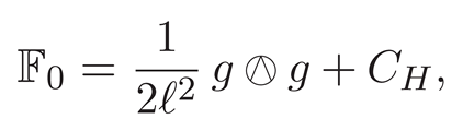where the first term is the constant-curvature gravitational reference and $C_H$ is the scalar zero-form reference. The jets are

$$\begin{array}{cccc}\hfill {\mathfrak{J}}_{ϵ}\psi & =\left(\psi +iϵD\psi ,\sqrt{ϵ}{\mathbb{D}}^2\right),\hfill & \hfill {\mathfrak{J}}_r\psi & =\left(\psi ,\sqrt{ϵ}{\mathbb{F}}_0\right).\hfill \end{array}$$

(123)

Choose the invariant curvature pairing sectorwise on the gravitational, gauge, Higgs-derivative, and scalar endomorphism components, including the allowed mixed invariant $\xi R{H}^{†}H$. Proposition 1 then gives

$$\mathcal{K}\left({\mathfrak{J}}_{ϵ}\psi ,{\mathfrak{J}}_r\psi \right)=-iϵS_{\mathrm{ESM}}+O\left({ϵ}^2\right),$$

(124)

and accumulating gives

$$\mathcal{I}=-i{S}_{\mathrm{ESM}},S_{\mathrm{ESM}}={\int }_X^{4}x\sqrt{-g}{\mathcal{L}}_{\mathrm{ESM}},$$

(125)

where

$$\begin{array}{cc}\hfill {\mathcal{L}}_{\mathrm{ESM}}& =a{C}_{\mu \nu \rho \sigma }{C}^{\mu \nu \rho \sigma }+b{R}^2+c{E}_4+{\displaystyle \frac{M_{\mathrm{P}}^2}{2}}R-\mathsf{\Lambda }\hfill \\ \hfill & -{\displaystyle \frac{1}{4g_3^2}}{G}_{\mu \nu }^A{G}^{A\mu \nu }-{\displaystyle \frac{1}{4g_2^2}}{W}_{\mu \nu }^I{W}^{I\mu \nu }-{\displaystyle \frac{1}{4g_1^2}}{B}_{\mu \nu }{B}^{\mu \nu }\hfill \\ \hfill & +\sum _f{\overline{\psi }}_{f}i{\gamma }^{\mu }{D}_{\mu }^{\mathrm{SM}}{\psi }_f-{\left(D_{\mu }^{\mathrm{SM}}H\right)}^{†}{D}^{\mu ,\mathrm{SM}}H-\xi R{H}^{†}H\hfill \\ \hfill & -m_H^2{H}^{†}H-{\lambda }_H{\left(H^{†}H\right)}^2\hfill \\ \hfill & -\left({\overline{Q}}_L{Y}_u\tilde{H}{u}_R+{\overline{Q}}_L{Y}_{d}H{d}_R+{\overline{L}}_L{Y}_{e}H{e}_R+{\overline{L}}_L{Y}_{\nu }\tilde{H}{\nu }_R+\mathrm{h}.\mathrm{c}.\right),\hfill \end{array}$$

(126)

with $\tilde{H}=i{\sigma }_2{H}^{*}$ — the Standard Model matter action coupled to Einstein–Stelle quadratic gravity.

3. Main Result

Having calibrated least surprisal against established Lagrangians, we now construct the spacetime transition jets, and determine the theory produced by their accumulated surprisal. Insofar as the jets describe spacetime transitions, the resulting theory is the least-surprising theory spacetime furnishes of itself.

3.1. The Arena

The dimensionality of surprisal fixes the arena and its signature.

Theorem 1 

(Dimensionality of surprisal). Let Ψ be a canonically normalized Dirac field in d spacetime dimensions, let the contracted transport have mass dimension one, and let its curvature and reference have mass dimension two:

$$\left[\mathsf{\Psi }\right]={\displaystyle \frac{d-1}{2}},\left[D\right]=1,\left[{\mathbb{D}}^2\right]=\left[{\mathbb{F}}_0\right]=2.$$

(127)

The local coefficients furnished by the matter and curvature slots then have dimensions

$$\begin{array}{cccc}\hfill \left[Re{\langle \mathsf{\Psi }\mid D\mathsf{\Psi }\rangle }_x\right]& =d,\hfill & \hfill \left[Q\left({\mathbb{D}}^2-{\mathbb{F}}_0,{\mathbb{D}}^2-{\mathbb{F}}_0\right)\right]& =4.\hfill \end{array}$$

(128)

Consequently, the two slots contribute to a common local Lagrangian with a dimensionless relative slot weight precisely when

$$d=4.$$

(129)

Equivalently, only in four dimensions does the given transition-jet pairing combine canonically normalized Dirac transport and curvature-square dynamics without an additional dimensionful relative coefficient.

Having selected $d=4$, the remaining metric signatures are

$$(4,0),(3,1),(2,2),(1,3),(0,4).$$

(130)

The matter slot furnishes the Dirac equation and its conserved current

$$J^{\mu }=\overline{\mathsf{\Psi }}{\gamma }^{\mu }\mathsf{\Psi }.$$

(131)

For this current to represent the locally measurable density of the amplitude, we require the existence of a unit covector n whose contraction with the current,

$$n_{\mu }{J}^{\mu },$$

(132)

is positive-definite in the orientation defined by n: nonvanishing for every nonzero physical state, with a common sign fixed to be positive by the choice of orientation. Any such n is necessarily timelike, and its existence defines the temporal orientation of the arena. The intrinsic Clifford-compatible Dirac adjoint admits such a positive-definite density in the one-time Lorentzian signatures

$$(3,1),(1,3),$$

(133)

which differ only by the overall metric-sign convention. In Euclidean signature the contraction is indefinite for every unit vector: $n·\gamma$ squares to the identity and is traceless, so its spectrum is symmetric about zero. In split signature the same failure occurs on the unrestricted Dirac carrier for every choice of n, timelike in either of the two temporal planes or otherwise.

The transition jets therefore select Lorentzian $3+1$ spacetime: four dimensions are required for dimensionless compatibility of their matter and curvature slots, and Lorentzian signature is required for the positive conserved density of the Dirac amplitude. The selected dimension is additionally the marginal dimension of curvature-square gravity and hence the dimension in which the resulting gravitational theory is power-counting renormalizable with dimensionless higher-curvature couplings.

3.2. The Carrier

We now collect the carrier structures supplied by the 3+1D arena.

For the jets of a carrier to describe the spacetime transitions, its amplitude, parameters, and representation spaces must be constructed from structures intrinsic to the geometry, without appending an unrelated internal vector space, symmetry group, or representation—otherwise it would describe the transitions of another geometry than spacetime, defeating the goal of identifying the least surprising theory of spacetime.

The initial local data are a point $x\in X$ and a Lorentzian metric $g_x$ on $T_{x}X$. Denote by ${\mathcal{M}}_{1,3}\left(X\right)$ the bundle of local Lorentzian metrics, whose points are pairs $(x,g_x)$. A metric field is a section $g\in \mathsf{\Gamma }\left({\mathcal{M}}_{1,3}\left(X\right)\right).$

Metric-fibre structure.

Retaining $g_x$ as a parameter supplies the tangent space to the local metric fibre,

$$V_{x,g}:=T_{g_x}{\mathcal{M}}_{1,3,x}\left(X\right)\cong {Sym}^2\left(T_x^{*}X\right),$$

(134)

equipped with the DeWitt form $G_{g_x}$. Since spacetime is four-dimensional,

$${dim}_{\mathbb{R}}{V}_{x,g}={dim}_{\mathbb{R}}{Sym}^2\left(T_x^{*}X\right)=10.$$

(135)

The quadratic space $(V_{x,g},G_{g_x})$ therefore supplies its Clifford algebra, spin-frame symmetry, and complex half-spin representations. These representations provide the internal particle carrier; no independent grand-unification space is introduced.

Spacetime-algebra structure.

In four-dimensional Lorentzian spacetime, the complex Dirac amplitude admits its Dirac–Hestenes realization as an even Clifford multivector. The corresponding real algebra satisfies

$${Cl}^{+}(T_{x}X,g_x)\cong {Mat}_2\left(\mathbb{C}\right).$$

(136)

Its eight real components agree with those of an ordinary four-component complex Dirac spinor.

Spacetime spin acts on this carrier from the left,

$$\psi ⟼S\psi ,S\in Spin(1,3),$$

(137)

while associativity permits an independent commuting right action,

$$\psi ⟼\psi U,S\left(\psi U\right)=\left(S\psi \right)U.$$

(138)

The admissible right action is fixed by invariance of the Dirac–Hestenes current

$$J\left(\psi \right):=\psi {\gamma }_0\tilde{\psi }.$$

(139)

Indeed,

$$J\left(\psi U\right)=\psi \left(U{\gamma }_0\tilde{U}\right)\tilde{\psi },$$

(140)

so $J\left(\psi U\right)=J\left(\psi \right)$ for every amplitude $\psi$ if and only if

$$U{\gamma }_0\tilde{U}={\gamma }_0.$$

(141)

The connected right stabilizer is generated by the three spatial bivectors ${\gamma }_i{\gamma }_j$, which generate $Spin\left(3\right)\cong SU\left(2\right)$, together with the spacetime pseudoscalar

$$I:={\gamma }_0{\gamma }_1{\gamma }_2{\gamma }_3,I^2=-1,$$

(142)

which generates a commuting $U\left(1\right)$ phase. Consequently,

$${Stab}_R{\left(J\right)}_0\cong {\displaystyle \frac{Spin\left(3\right)\times U\left(1\right)}{{\mathbb{Z}}_2}}\cong {\displaystyle \frac{SU\left(2\right)\times U\left(1\right)}{{\mathbb{Z}}_2}}\cong U\left(2\right).$$

(143)

We denote this uniquely selected connected current-preserving right group by

$$U{\left(2\right)}_{\mathrm{fam}}.$$

(144)

We retain its coordinate

$$u\in U{\left(2\right)}_{\mathrm{fam}}$$

(145)

as an argument of the complete amplitude. Its subsequent reduction and spectral resolution determine the family sector.

Definition 5 

(The carrier of spacetime). Let X be a four-dimensional Lorentzian manifold, let

$$V_{x,g}:=T_{g_x}{\mathcal{M}}_{1,3,x}\left(X\right)\cong {Sym}^2\left(T_x^{*}X\right),$$

(146)

and let $U{\left(2\right)}_{\mathrm{fam}}$ be the commuting nongauged right-action group intrinsic to the spacetime-algebra factor. The native carrier of spacetime is the amplitude

$$\mathsf{\Psi }=\mathsf{\Psi }(x,g_x,u),(x,g_x)\in {\mathcal{M}}_{1,3}\left(X\right),u\in U{\left(2\right)}_{\mathrm{fam}},$$

(147)

with pointwise values

$$\mathsf{\Psi }(x,g_x,u)\in {Cl}^{+}(T_{x}X,g_x)\otimes {\mathsf{\Sigma }}^{\epsilon }\left(V_{x,g},G_{g_x}\right),\epsilon \in \{+,-\}.$$

(148)

Here ${Cl}^{+}(T_{x}X,g_x)$ is the real Dirac–Hestenes spacetime carrier. The symbol $\mathsf{\Sigma }(V_{x,g},G_{g_x})$ denotes the complex spin module associated with the metric-variation quadratic space. Since ${dim}_{\mathbb{R}}{V}_{x,g}=10$ is even, its restriction to the even Clifford algebra decomposes into irreducible chiral half-spin modules,

$$\mathsf{\Sigma }(V_{x,g},G_{g_x})={\mathsf{\Sigma }}^{+}(V_{x,g},G_{g_x})\oplus {\mathsf{\Sigma }}^{-}(V_{x,g},G_{g_x}),$$

(149)

and ${\mathsf{\Sigma }}^{\epsilon }$ denotes one selected irreducible chirality. Reversal of the fibre orientation exchanges the two choices.

The carrier of spacetime thus combines two independent internal structures, both supplied by its geometric factors:

$$U{\left(2\right)}_{\mathrm{fam}}\mathrm{and}Spin(V_{x,g},G_{g_x}).$$

(150)

The first is the nongauged right-action structure of the spacetime-algebra factor and will determine family multiplicity. The second is the spin-frame symmetry of the metric-variation factor and will determine the particle gauge representation. Both groups are retained unreduced in Definition 5; their reductions and physical consequences are derived in the subsequent subsections.

Remark 2 

(Pointwise and global carriers). Definition 5 is pointwise over $(x,g_x)$ and retains functional dependence on the nongauged family coordinate u. Its globalization requires the corresponding Clifford and fibre-spinor bundles, together with the appropriate spin or ${Spin}^c$ lifts. These global topological conditions are assumed whenever the pointwise carriers are assembled into bundles.

3.3. The Particle Sector

The local metric fibre of 3+1D has tangent space

$$V_{x,g}=T_{g_x}{\mathcal{M}}_{1,3,x}\left(X\right)\cong {Sym}^2\left(T_x^{*}X\right),dim{V}_{x,g}=10.$$

(151)

Its DeWitt form determines the ambient spin-frame symmetry of the internal carrier.

Lemma 1 

(DeWitt signature). Let

$$G_g(h,k)=h_{\mu \nu }{k}_{\rho \sigma }\left[g^{\mu \rho }{g}^{\nu \sigma }-\lambda g^{\mu \nu }{g}^{\rho \sigma }\right]$$

(152)

on

$$V_{x,g}={Sym}^2\left(T_x^{*}X\right),$$

(153)

where g is Lorentzian and $\lambda >1/d$. Then

$$dim{V}_{x,g}={\displaystyle \frac{d(d+1)}{2}},sig{G}_g=\left({\displaystyle \frac{d(d-1)}{2}},d\right).$$

(154)

In the selected arena $d=4$, and therefore

$$dim{V}_{x,g}=10,sig{G}_g=(6,4).$$

(155)

At $\lambda =1/d$, the trace direction is null.

Proof. 

Decompose a metric variation into its trace and traceless parts:

$$h=h_0+{\displaystyle \frac{{tr}_{g}h}{d}}g,{tr}_g{h}_0=0.$$

(156)

The decomposition is orthogonal with respect to $G_g$. In a Lorentzian orthonormal frame, the $d-1$ off-diagonal components containing one temporal index have negative norm, while the remaining off-diagonal components have positive norm. The trace direction has norm

$$G_g(g,g)=d-\lambda d^2,$$

(157)

which is negative for $\lambda >1/d$. Counting the resulting positive and negative directions gives

$$sig{G}_g=\left({\displaystyle \frac{d(d-1)}{2}},d\right).$$

(158)

Setting $d=4$ gives $(6,4)$. □

3+1D therefore supplies

$$Spin(V_{x,g},G_{g_x})\cong Spin(6,4).$$

(159)

Positive definiteness of the fibre-spin particle density selects a positive polarization

$$R_x^2=\mathbb{1},G_{g_x}(u,R_{x}u)>0,$$

(160)

and hence the maximal compact symmetry

$$Spin(6,4)⟶Spin\left(6\right)\times Spin\left(4\right)\cong SU\left(4\right)\times SU{\left(2\right)}_L\times SU{\left(2\right)}_R,$$

(161)

the Pati–Salam group.

To develop the experimentally established Standard Model realization, we impose two additional structures: a compatible complex structure $J_x$ and unimodularity,

$$J_x^2=-\mathbb{1},G_{g_x}(J_{x}u,J_{x}v)=G_{g_x}(u,v),[J_x,R_x]=0.$$

(162)

The common stabilizer of $R_x$ and $J_x$ is

$$U\left(3\right)\times U\left(2\right),$$

(163)

and unimodularity reduces it to

$$S\left(U\left(3\right)\times U\left(2\right)\right)\cong {\displaystyle \frac{SU{\left(3\right)}_c\times SU{\left(2\right)}_L\times U{\left(1\right)}_Y}{{\mathbb{Z}}_6}},$$

(164)

the faithful Standard Model gauge group. Its central generator is, up to normalization and sign,

$$Y=diag\left(-{\displaystyle \frac{1}{3}},-{\displaystyle \frac{1}{3}},-{\displaystyle \frac{1}{3}},{\displaystyle \frac{1}{2}},{\displaystyle \frac{1}{2}}\right).$$

(165)

Thus the internal reductions are

$$\begin{array}{|c|}\hline Spin(6,4)\stackrel{R_x}{\to }{G}_{\mathrm{PS}}\stackrel{J_x}{\to }U\left(3\right)\times U\left(2\right)\stackrel{\mathrm{unimodularity}}{\to }{G}_{\mathrm{SM}}.\\ \hline\end{array}$$

(166)

3.4. The Family Sector

Definition 5 retains the full dependence

$$\mathsf{\Psi }=\mathsf{\Psi }(x,g_x,u),u\in U{\left(2\right)}_{\mathrm{fam}},$$

(167)

on the nongauged right-action geometry of the spacetime-algebra factor. We now reduce this already-present family dependence and determine its spectrum.

Select the maximal-torus subgroup

$$H_{\mathrm{fam}}:=U\left(1\right)\times U\left(1\right)\subset U{\left(2\right)}_{\mathrm{fam}}.$$

(168)

The corresponding homogeneous space is

$${\mathcal{Y}}_{\mathrm{fam}}:={\displaystyle \frac{U{\left(2\right)}_{\mathrm{fam}}}{H_{\mathrm{fam}}}}\cong {\mathbb{CP}}^1\cong S^2.$$

(169)

Because $U{\left(2\right)}_{\mathrm{fam}}$ is nongauged, the residual $H_{\mathrm{fam}}$ does not enlarge the particle gauge group or introduce additional gauge fields.

Let

$$h=diag\left(e^{i\alpha },e^{i\beta }\right)\in H_{\mathrm{fam}}.$$

(170)

The holomorphic tangent direction of the orbit transforms under the isotropy character

$${\chi }_{\tan }\left(h\right)=e^{i(\alpha -\beta )},$$

(171)

up to reversal of the complex orientation. We select from the original u-dependent carrier the tangent-equivariant sector satisfying

$$\mathsf{\Psi }(x,g_x,uh)={\chi }_{\tan }{\left(h\right)}^{-1}\mathsf{\Psi }(x,g_x,u).$$

(172)

Equivariant functions of this type are canonically identified with sections of the associated bundle

$$U{\left(2\right)}_{\mathrm{fam}}{\times }_{H_{\mathrm{fam}}}{\mathbb{C}}_{\tan }\cong T^{1,0}{\mathcal{Y}}_{\mathrm{fam}}\cong T^{1,0}{\mathbb{CP}}^1\cong \mathcal{O}\left(2\right).$$

(173)

Thus the family reduction does not append a new carrier factor: it selects a geometrically distinguished sector of the $U{\left(2\right)}_{\mathrm{fam}}$ dependence already contained in Definition 5.

The corresponding first-order family transport is the Dolbeault–Dirac operator

$$D_{\mathrm{fam}}:={\displaystyle \frac{\sqrt{2}}{r_{\mathrm{f}}}}\left({\overline{\partial }}_{\mathcal{O}\left(2\right)}+{\overline{\partial }}_{\mathcal{O}\left(2\right)}^{†}\right),$$

(174)

where $r_{\mathrm{f}}$ is the geometric scale of the family orbit. Because the family symmetry is independent of the metric-fibre particle symmetry, this operator acts trivially on the particle representation:

$$\left[D_{\mathrm{fam}},\rho \left(G_{\mathrm{SM}}\right)\right]=0.$$

(175)

Theorem 2 

(Three chiral family modes). The tangent-equivariant family operator (174) has three positive-chirality zero modes and no negative-chirality zero modes:

$${dim}_{\mathbb{C}}ker{D}_{\mathrm{fam}}^{+}=3,{dim}_{\mathbb{C}}ker{D}_{\mathrm{fam}}^{-}=0.$$

(176)

Its chiral index is therefore

$$ind{D}_{\mathrm{fam}}^{+}=3.$$

(177)

Proof. 

For the degree-two line bundle on ${\mathbb{CP}}^1$,

$$\begin{array}{cccc}\hfill H^0\left({\mathbb{CP}}^1,\mathcal{O}\left(2\right)\right)& \cong {\mathbb{C}}^3,\hfill & \hfill H^1\left({\mathbb{CP}}^1,\mathcal{O}\left(2\right)\right)& =0.\hfill \end{array}$$

(178)

Equivalently, Riemann–Roch gives

$$\chi \left({\mathbb{CP}}^1,\mathcal{O}\left(2\right)\right)=deg\mathcal{O}\left(2\right)+1=3.$$

(179)

The positive- and negative-chirality kernels of the Dolbeault–Dirac operator are represented by $H^0$ and $H^1$, respectively. The vanishing of $H^1$ therefore shows that the index counts three actual positive-chirality zero modes. □

Define the family zero-mode space by

$${\mathcal{F}}_{\mathrm{fam}}:=ker{D}_{\mathrm{fam}}^{+}\cong {\mathbb{C}}^3.$$

(180)

If $F^{+}$ denotes the chiral metric-fibre module containing the particle content of one generation, then

$${\mathcal{F}}_{\mathrm{fam}}\otimes F^{+}\cong {\mathbb{C}}^3\otimes F^{+}\cong 3F^{+}.$$

(181)

Because the family operator commutes with the particle gauge action, the three factors have identical Standard Model quantum numbers. The metric-fibre geometry determines the content of one generation, while the nongauged STA family geometry determines its multiplicity.

The family operator also has a discrete nonzero spectrum. Let

$$D_{\mathrm{fam}}{\chi }_n=0,n=1,2,3,$$

(182)

and

$$D_{\mathrm{fam}}{\chi }_{\alpha }={\lambda }_{\alpha }{\chi }_{\alpha },{\lambda }_{\alpha }\ne 0,$$

(183)

denote orthonormal zero and nonzero modes. The original u-dependent amplitude then has the reduced spectral expansion

$$\mathsf{\Psi }(x,g_x,u)={\displaystyle \sum _{n=1}^3}{\mathsf{\Psi }}_n(x,g_x){\chi }_n\left(u\right)+\sum _{{\lambda }_{\alpha }\ne 0}{\mathsf{\Psi }}_{\alpha }(x,g_x){\chi }_{\alpha }\left(u\right).$$

(184)

When $D_{\mathrm{fam}}$ is included in the total contracted transport, the first sum gives three chiral generations, while the second gives a tower of family excitations with characteristic scale

$$m_{\alpha }^{\mathrm{fam}}\sim \left|{\lambda }_{\alpha }\right|\sim r_{\mathrm{f}}^{-1}.$$

(185)

The family zero-mode condition does not make the observed fermions massless: their four-dimensional masses arise from the Higgs Yukawa and possible Majorana transports assembled below.

Family dependence of the scalar transport produces the Yukawa and Majorana matrices through overlap integrals. For example,

$${\left(Y_f\right)}_{mn}={\int }_{{\mathcal{Y}}_{\mathrm{fam}}}{\mu }_{\mathrm{f}}〈{\chi }_m\left|{\mathsf{\Phi }}_f\right|{\chi }_n〉,f=u,d,e,\nu ,$$

(186)

with an analogous expression for $M_R$. Their relative diagonalizations yield the CKM and PMNS matrices.

The resulting division of roles is

$$\begin{array}{|c|}\hline \begin{array}{cc}\hfill {\mathsf{\Sigma }}^{+}(V_{x,g},G_{g_x})& ⟶\mathrm{particle}\mathrm{content}\mathrm{of}\mathrm{one}\mathrm{generation},\hfill \\ \hfill ind{D}_{\mathrm{fam}}^{+}=3& ⟶\mathrm{three}\mathrm{chiral}\mathrm{generations},\hfill \\ \hfill \mathrm{family}-\mathrm{dependent}\mathrm{scalar}\mathrm{transport}& ⟶\mathrm{masses}\mathrm{and}\mathrm{flavour}\mathrm{mixing}.\hfill \end{array}\\ \hline\end{array}$$

(187)

3.5. Assembly

The preceding results determine the particle and family structures of the carrier. After the family reduction, the same amplitude defined in Definition 5 is written as

$$\mathsf{\Psi }=\mathsf{\Psi }(x,g_x,y),y\in {\mathcal{Y}}_{\mathrm{fam}}\cong {\mathbb{CP}}^1,$$

(188)

where the reduced y dependence is valued in

$$T^{1,0}{\mathcal{Y}}_{\mathrm{fam}}\cong \mathcal{O}\left(2\right).$$

(189)

The spacetime action is evaluated along a physical metric section $g\in \mathsf{\Gamma }\left({\mathcal{M}}_{1,3}\left(X\right)\right)$, while the complete family dependence is retained.

The metric-fibre half-spin module $F^{+}$ contains one complete Standard Model generation, while the family operator supplies

$${\mathcal{F}}_{\mathrm{fam}}:=ker{D}_{\mathrm{fam}}^{+}\cong {\mathbb{C}}^3.$$

(190)

Because the nongauged family transport commutes with the Standard Model action, the three-generation zero-mode carrier is

$${\mathcal{E}}_{\mathrm{f}}^{\left(3\right)}={\mathcal{F}}_{\mathrm{fam}}\otimes \left[(S_L\otimes F_L)\oplus (S_R\otimes F_R)\right],$$

(191)

where

$$F_L=Q_L\oplus L_L,F_R=u_R\oplus d_R\oplus {\nu }_R\oplus e_R.$$

(192)

For the complex-polarized and unimodular realization of Section 3.3, let

$${\nabla }_{g,A}={\nabla }_g^{\mathrm{spin}}+{\nabla }_A^{\mathrm{SM}}$$

(193)

denote the spacetime and particle-gauge transport, where

$$G_{\mathrm{SM}}=S\left(U\left(3\right)\times U\left(2\right)\right)\cong {\displaystyle \frac{SU{\left(3\right)}_c\times SU{\left(2\right)}_L\times U{\left(1\right)}_Y}{{\mathbb{Z}}_6}}.$$

(194)

The family transport is the Dolbeault transport on $\mathcal{O}\left(2\right)\to {\mathbb{CP}}^1$, whose contracted operator is

$$D_{\mathrm{fam}}={\displaystyle \frac{\sqrt{2}}{r_{\mathrm{f}}}}\left({\overline{\partial }}_{\mathcal{O}\left(2\right)}+{\overline{\partial }}_{\mathcal{O}\left(2\right)}^{†}\right).$$

(195)

Here $r_{\mathrm{f}}$ sets the family-excitation scale. Since the family structure is nongauged and independent of the metric-fibre particle symmetry,

$$\left[D_{\mathrm{fam}},\rho \left(G_{\mathrm{SM}}\right)\right]=0.$$

(196)

The minimal odd Lorentz-scalar transport connecting the left- and right-handed matter sectors is the Higgs zero-form

$${\mathsf{\Phi }}_H=\left(\begin{array}{cc}0& {\mathsf{\Phi }}_{LR}\left(H\right)\\ {\mathsf{\Phi }}_{LR}{\left(H\right)}^{†}& 0\end{array}\right),H\sim {(\mathbf{1},\mathbf{2})}_{1/2},\tilde{H}:=i{\sigma }_2{H}^{*},$$

(197)

with

$${\mathsf{\Phi }}_{LR}\left(H\right)\sim diag\left({\mathcal{Y}}_u\left(y\right)\tilde{H},{\mathcal{Y}}_d\left(y\right)H,{\mathcal{Y}}_{\nu }\left(y\right)\tilde{H},{\mathcal{Y}}_e\left(y\right)H\right).$$

(198)

The operators ${\mathcal{Y}}_f\left(y\right)$ act on the family dependence. If ${\left\{{\chi }_n\right\}}_{n=1}^3$ is an orthonormal basis of $ker{D}_{\mathrm{fam}}^{+}$, their restrictions to the zero-mode sector give the physical Yukawa matrices

$${\left(Y_f\right)}_{mn}={\int }_{{\mathcal{Y}}_{\mathrm{fam}}}{\mu }_{\mathrm{f}}\left(y\right)〈{\chi }_m\left(y\right)\left|{\mathcal{Y}}_f\left(y\right)\right|{\chi }_n\left(y\right)〉,f=u,d,e,\nu .$$

(199)

The complete generalized transport and its Clifford contraction are

$$\begin{array}{cc}\hfill {\mathbb{D}}_{\mathrm{tot}}& ={\nabla }_{g,A}+{\mathbb{D}}_{\mathrm{fam}}+{\mathsf{\Phi }}_H,\hfill \end{array}$$

(200)

$$\begin{array}{cc}\hfill D_{\mathrm{tot}}& =i{\gamma }^{\mu }{\nabla }_{g,A,\mu }+{\gamma }_5{D}_{\mathrm{fam}}-{\mathsf{\Phi }}_H.\hfill \end{array}$$

(201)

The factor ${\gamma }_5$ supplies the grading of the product Dirac operator.

The corresponding supercurvature decomposes as

$$\begin{array}{cc}\hfill {\mathbb{D}}_{\mathrm{tot}}^2& =\underset{\mathrm{spacetime}\mathrm{curvature}}{\underbrace{R_g}}+\underset{\mathrm{gauge}\mathrm{curvature}}{\underbrace{F_A^{\mathrm{SM}}}}+\underset{\mathrm{family}\mathrm{curvature}}{\underbrace{F_{\mathrm{fam}}}}\hfill \\ \hfill & +\underset{\mathrm{horizontal}--\mathrm{family}\mathrm{curvature}}{\underbrace{F_{\mathrm{mix}}}}+\underset{\mathrm{horizontal}\mathrm{Higgs}\mathrm{transport}}{\underbrace{D_{g,A}{\mathsf{\Phi }}_H}}+\underset{\mathrm{family}\mathrm{Higgs}\mathrm{transport}}{\underbrace{D_{\mathrm{fam}}{\mathsf{\Phi }}_H}}+\underset{\mathrm{zero}-\mathrm{form}}{\underbrace{{\mathsf{\Phi }}_H^2}},\hfill \end{array}$$

(202)

where

$$\begin{array}{cccc}\hfill F_{\mathrm{fam}}& :={\mathbb{D}}_{\mathrm{fam}}^2,\hfill & \hfill F_{\mathrm{mix}}& :=[{\nabla }_{g,A},{\mathbb{D}}_{\mathrm{fam}}],\hfill \end{array}$$

(203)

$$\begin{array}{cccc}\hfill D_{g,A}{\mathsf{\Phi }}_H& :=[{\nabla }_{g,A},{\mathsf{\Phi }}_H],\hfill & \hfill D_{\mathrm{fam}}{\mathsf{\Phi }}_H& :=[{\mathbb{D}}_{\mathrm{fam}},{\mathsf{\Phi }}_H].\hfill \end{array}$$

(204)

For the product transport considered here,

$$F_{\mathrm{mix}}=0.$$

(205)

The family dependence of ${\mathsf{\Phi }}_H$ remains nontrivial and produces the Yukawa matrices and flavour mixing.

The basic curvature pairing is sectorwise on the gravitational, Standard Model gauge, family, Higgs-derivative, and scalar components. The complete renormalizable pairing additionally admits the mixed invariant

$${〈R_g,{\mathsf{\Phi }}_H^2〉}_{\mathrm{mix}}:=\xi R{H}^{†}H.$$

(206)

The reference contains gravitational, family, and scalar components:

(207)

The first term is the constant-curvature gravitational reference, $F_{\mathrm{fam},0}$ is the family curvature declared unsurprising, and $C_H$ is the scalar vacuum reference. For the fixed nongauged family geometry, one may take

$$F_{\mathrm{fam},0}=F_{\mathrm{fam}},$$

(208)

so its background curvature does not produce an additional dynamical gauge sector.

The spacetime displacement and reference jets are

$$\begin{array}{cc}\hfill {\mathfrak{J}}_{ϵ}\mathsf{\Psi }& =\left(\mathsf{\Psi }+iϵD_{\mathrm{tot}}\mathsf{\Psi },\sqrt{ϵ}{\mathbb{D}}_{\mathrm{tot}}^2\right),\hfill \end{array}$$

(209)

$$\begin{array}{cc}\hfill {\mathfrak{J}}_r\mathsf{\Psi }& =\left(\mathsf{\Psi },\sqrt{ϵ}{\mathbb{F}}_{0,\mathrm{tot}}\right).\hfill \end{array}$$

(210)

By Proposition 1, their accumulated surprisal is

$${\mathcal{I}}_{\mathrm{tot}}=-i{S}_{\mathrm{tot}},$$

(211)

with

$$\begin{array}{cc}\hfill S_{\mathrm{tot}}& ={\int }_X{\mathrm{d}}^{4}x\sqrt{-g}{\int }_{{\mathcal{Y}}_{\mathrm{fam}}}{\mu }_{\mathrm{f}}\left(y\right)[Re{〈\mathsf{\Psi }|D_{\mathrm{tot}}\mathsf{\Psi }〉}_{x,y}\hfill \\ \hfill & +{\displaystyle \frac{s_F}{2}}{〈{\mathbb{D}}_{\mathrm{tot}}^2-{\mathbb{F}}_{0,\mathrm{tot}},{\mathbb{D}}_{\mathrm{tot}}^2-{\mathbb{F}}_{0,\mathrm{tot}}〉}_{x,y}-\xi R{H}^{†}H].\hfill \end{array}$$

(212)

The family measure is normalized by

$${\int }_{{\mathcal{Y}}_{\mathrm{fam}}}{\mu }_{\mathrm{f}}=1,$$

(213)

while the physical family scale is carried by $r_{\mathrm{f}}$.

The curvature comparison decomposes as

(214)

Its invariant pairings supply

(215)

$$\begin{array}{cc}\hfill F_A^{\mathrm{SM}}& ⟼G_{\mu \nu }^A{G}^{A\mu \nu },W_{\mu \nu }^I{W}^{I\mu \nu },B_{\mu \nu }{B}^{\mu \nu },\hfill \end{array}$$

(216)

$$\begin{array}{cc}\hfill D_{g,A}{\mathsf{\Phi }}_H& ⟼-{\left(D_{\mu }H\right)}^{†}{D}^{\mu }H,\hfill \end{array}$$

(217)

$$\begin{array}{cc}\hfill D_{\mathrm{fam}}{\mathsf{\Phi }}_H& ⟼\mathrm{family}\text{-}\mathrm{dependent}\mathrm{scalar}\mathrm{transport},\hfill \end{array}$$

(218)

$$\begin{array}{cc}\hfill {\mathsf{\Phi }}_H^2-C_H& ⟼-m_H^2{H}^{†}H-{\lambda }_H{\left(H^{†}H\right)}^2.\hfill \end{array}$$

(219)

Together with (206), these are the gravitational, gauge, scalar, and family operators of the assembled theory.

Let

$$\begin{array}{cccc}\hfill D_{\mathrm{fam}}{\chi }_n& =0,\hfill & \hfill n& =1,2,3,\hfill \end{array}$$

(220)

$$\begin{array}{cccc}\hfill D_{\mathrm{fam}}{\chi }_{\alpha }& ={\lambda }_{\alpha }{\chi }_{\alpha },\hfill & \hfill {\lambda }_{\alpha }& \ne 0,\hfill \end{array}$$

(221)

be the zero and nonzero family modes. The amplitude has the spectral expansion

$$\mathsf{\Psi }(x,g_x,y)={\displaystyle \sum _{n=1}^3}{\psi }_n(x,g_x){\chi }_n\left(y\right)+\sum _{{\lambda }_{\alpha }\ne 0}{\psi }_{\alpha }(x,g_x){\chi }_{\alpha }\left(y\right).$$

(222)

The first sum gives three chiral Standard Model generations. The second gives a discrete tower of family excitations with characteristic scale

$$m_{\alpha }^{\mathrm{fam}}\sim \left|{\lambda }_{\alpha }\right|\sim r_{\mathrm{f}}^{-1}.$$

(223)

The zero family eigenvalue fixes generation multiplicity; ordinary fermion masses arise from the Yukawa matrices (199).

Because ${\nu }_R$ is a Standard Model singlet, the zero-form sector may also contain a symmetric Majorana matrix

$$M_R=M_R^T\in {Mat}_3\left(\mathbb{C}\right),$$

(224)

whose entries may likewise arise from family-mode overlaps. Setting $M_R=0$ leaves Dirac neutrinos, while $M_R\ne 0$ permits a type-I seesaw regime.

Restriction of (212) to $ker{D}_{\mathrm{fam}}^{+}$ gives the three-generation Standard Model coupled to quadratic gravity. Retaining the nonzero family spectrum gives the larger theory containing its excited family states. The explicit action is collected in Section 3.6.

3.6. The Action

Evaluating the sectors assembled in Section 3.5 gives the accumulated surprisal

$${\mathcal{I}}_{\mathrm{tot}}=\underset{ϵ\to 0}{lim}{\displaystyle \frac{1}{ϵ}}\mathcal{K}\left({\mathfrak{J}}_{ϵ}\mathsf{\Psi },{\mathfrak{J}}_r\mathsf{\Psi }\right)=-i{S}_{\mathrm{tot}}.$$

(225)

Because the amplitude retains its dependence on the family orbit, the complete action is accumulated over both spacetime and family space:

$$S_{\mathrm{tot}}={\int }_X^{4}x\sqrt{-g}{\int }_{{\mathcal{Y}}_{\mathrm{fam}}}{\mu }_{\mathrm{f}}\left(y\right){\mathcal{L}}_{\mathrm{tot}}(x,y),{\mathcal{Y}}_{\mathrm{fam}}\cong {\mathbb{CP}}^1.$$

(226)

The family measure is normalized by

$${\int }_{{\mathcal{Y}}_{\mathrm{fam}}}{\mu }_{\mathrm{f}}\left(y\right)=1,$$

(227)

while the physical family-excitation scale is carried by $r_{\mathrm{f}}$ in $D_{\mathrm{fam}}$.

Expanding the amplitude in eigenmodes of the family operator and performing the family integral decomposes the complete action as

$$S_{\mathrm{tot}}=S_{\mathrm{SM}+\mathrm{QG}}^{\left(3\right)}+S_{\mathrm{fam}}^{\mathrm{exc}},$$

(228)

where $S_{\mathrm{SM}+\mathrm{QG}}^{\left(3\right)}$ is the restriction to the three chiral family zero modes and $S_{\mathrm{fam}}^{\mathrm{exc}}$ contains the nonzero family spectrum.

The zero-mode action is

$$\begin{array}{cc}\hfill S_{\mathrm{SM}+\mathrm{QG}}^{\left(3\right)}& ={\int }_X{\mathrm{d}}^{4}x\sqrt{-g}[a{C}_{\mu \nu \rho \sigma }{C}^{\mu \nu \rho \sigma }+b{R}^2+c{E}_4+{\displaystyle \frac{M_{\mathrm{P}}^2}{2}}R-\mathsf{\Lambda }\hfill \\ \hfill & -{\displaystyle \frac{1}{4g_3^2}}{G}_{\mu \nu }^A{G}^{A\mu \nu }-{\displaystyle \frac{1}{4g_2^2}}{W}_{\mu \nu }^I{W}^{I\mu \nu }-{\displaystyle \frac{1}{4g_1^2}}{B}_{\mu \nu }{B}^{\mu \nu }\hfill \\ \hfill & +\sum _f{\overline{\psi }}_{f}i{\gamma }^{\mu }{D}_{\mu }^{\mathrm{SM}}{\psi }_f-{\left(D_{\mu }^{\mathrm{SM}}H\right)}^{†}{D}^{\mu ,\mathrm{SM}}H-\xi R{H}^{†}H\hfill \\ \hfill & -m_H^2{H}^{†}H-{\lambda }_H{\left(H^{†}H\right)}^2\hfill \\ \hfill & -\left({\overline{Q}}_L{Y}_u\tilde{H}{u}_R+{\overline{Q}}_L{Y}_{d}H{d}_R+{\overline{L}}_L{Y}_{e}H{e}_R+{\overline{L}}_L{Y}_{\nu }\tilde{H}{\nu }_R+\mathrm{h}.\mathrm{c}.\right)\hfill \\ \hfill & -{\displaystyle \frac{1}{2}}\left(\overline{{\nu }_R^c}{M}_R{\nu }_R+\mathrm{h}.\mathrm{c}.\right)],\hfill \end{array}$$

(229)

where

$$\tilde{H}=i{\sigma }_2{H}^{*}.$$

(230)

The fermion fields in (229) are vectors in the three-dimensional family zero-mode space. Accordingly,

$$Y_u,Y_d,Y_e,Y_{\nu },M_R\in {Mat}_3\left(\mathbb{C}\right),M_R=M_R^T.$$

(231)

The family integration in (226) supplies these matrices through the overlap integrals established in Section 3.5. Orthonormality of the family zero modes similarly reduces their kinetic pairing to the sum over three generations.

Because ${\nu }_R$ is a Standard Model singlet, the Majorana block $M_R$ is gauge invariant. Setting $M_R=0$ gives the Dirac-neutrino realization, while $M_R\ne 0$ permits a type-I seesaw regime. Its presence and scale remain zero-form transport or reference data.

The nonzero family modes contribute

$$S_{\mathrm{fam}}^{\mathrm{exc}}\supset \sum _{{\lambda }_{\alpha }\ne 0}{\int }_X^{4}x\sqrt{-g}{\overline{\psi }}_{\alpha }\left(i{\gamma }^{\mu }{D}_{\mu }^{\mathrm{SM}}+{\gamma }_5{\lambda }_{\alpha }\right){\psi }_{\alpha }+S_{\mathrm{fam}}^{\mathrm{int}},$$

(232)

where $S_{\mathrm{fam}}^{\mathrm{int}}$ contains the interactions obtained from family-dependent scalar transport. Their characteristic scale is

$$m_{\alpha }^{\mathrm{fam}}\sim \left|{\lambda }_{\alpha }\right|\sim r_{\mathrm{f}}^{-1}.$$

(233)

Thus the three observed generations are the chiral zero modes of the family operator, while the complete carrier also contains a discrete tower of nongauged family excitations.

The three-generation zero-mode theory is quantized perturbatively by the standard background-field and BRST treatment of quadratic gravity (Salvio, 2018; Stelle, 1977). One expands the metric and gauge fields about backgrounds,

$$g_{\mu \nu }={\overline{g}}_{\mu \nu }+\kappa h_{\mu \nu },A_{\mu }={\overline{A}}_{\mu }+a_{\mu },$$

(234)

and supplements the action by covariant gauge-fixing and ghost terms,

$$S_{\mathrm{gf}}=S_{\mathrm{SM}+\mathrm{QG}}^{\left(3\right)}+S_{\mathrm{g}.\mathrm{f}.}^{\mathrm{diff}}+S_{\mathrm{g}.\mathrm{f}.}^{\mathrm{SM}}+S_{\mathrm{gh}}^{\mathrm{diff}}+S_{\mathrm{gh}}^{\mathrm{SM}}.$$

(235)

The perturbative generating functional is then

$$Z[\overline{g},\overline{A}]=\int \mathcal{D}h\mathcal{D}a\mathcal{D}H\mathcal{D}\psi \mathcal{D}\overline{\psi }\mathcal{D}c\mathcal{D}\overline{c}{e}^{i{S}_{\mathrm{gf}}},$$

(236)

with the usual Feynman boundary conditions understood.

After four-derivative gravitational gauge fixing, the spin-two part of the propagator has the schematic form

$${\mathsf{\Delta }}^{\left(2\right)}\left(k\right)\propto {\displaystyle \frac{P^{\left(2\right)}}{k^2\left(1-k^2/m_2^2\right)}}=P^{\left(2\right)}\left[{\displaystyle \frac{1}{k^2}}-{\displaystyle \frac{1}{k^2-m_2^2}}\right],$$

(237)

with the pole prescription understood. Its ultraviolet behaviour is

$${\mathsf{\Delta }}^{\left(2\right)}\left(k\right)\sim {\displaystyle \frac{1}{k^4}},\left|k^2\right|⟶\infty ,$$

(238)

which yields the power-counting renormalizability of the four-dimensional curvature-square operator basis. The opposite residue of the massive spin-two pole is represented by an opposite-norm sector of the state space. The resulting kinematical carrier is therefore of Hilbert–Krein form,

$$K_{universe}={\mathcal{H}}_{\mathrm{SM}}^{\left(3\right)}\widehat{\otimes }{K}_{\mathrm{QG}},{\eta }_{universe}={\mathbb{1}}_{\mathrm{SM}}^{\left(3\right)}\otimes {\eta }_{\mathrm{QG}},$$

(239)

whose intensity-positive measurement interpretation is developed in the next section.

4. Intensity Measurements

One difficulty remains. The quadratic-gravity action is perturbatively renormalizable and admits asymptotically free trajectories (Avramidi and Barvinsky, 1985; Fradkin and Tseytlin, 1982; Salvio, 2018; Stelle, 1977), but its standard covariant quantization contains a massive spin-two pole with opposite residue. This pole is not an incidental excitation that can simply be removed: schematically,

$${\displaystyle \frac{1}{k^2(1+k^2/m_2^2)}}={\displaystyle \frac{1}{k^2}}-{\displaystyle \frac{1}{k^2+m_2^2}},$$

(240)

so the same pole that produces the indefinite sector is tied to the $k^{-4}$ ultraviolet decay underlying perturbative renormalizability.

Retaining the complete spectrum therefore places the massive spin-two mode in a negative-metric sector, conventionally called the Stelle ghost. Since the Standard Model sector is Hilbert-positive, the resulting kinematical carrier is

$$\begin{array}{|c|}\hline K_{universe}={\mathcal{H}}_{\mathrm{SM}}^{\left(3\right)}\widehat{\otimes }{K}_{\mathrm{QG}},{\eta }_{universe}={\mathbb{1}}_{\mathrm{SM}}^{\left(3\right)}\otimes {\eta }_{\mathrm{QG}},\\ \hline\end{array}$$

(241)

where ${\eta }_{\mathrm{QG}}$ acts as $+\mathbb{1}$ on the positive sectors and as $-\mathbb{1}$ on the massive spin-two sector.

The usual objection conflates measurement with a globally normalized probability measure, and as such incorrectly claims that measurements are not possible on a Krein space. The literature is a prescription of attempts to remove the ghost without damaging the renormalizable character of the theory. However, a simpler realization resolves the issue—the physical interpretation is merely that Hilbert spaces describe quantum systems with external observers, and Krein spaces describe quantum systems with internal observers.

A probability measure satisfies three Kolmogorov requirements: nonnegativity, countable additivity on disjoint channels, and normalization of an exhaustive family to unity. However, detector records prior to normalization are intensities, which require only the first two:

$$I_A\left(\omega \right)\ge 0,I_{{\sum }_m{A}_m}\left(\omega \right)=\sum _m{I}_{A_m}\left(\omega \right).$$

(242)

Whenever a registered family $\mathcal{D}=\left\{A_m\right\}$ has finite nonzero total intensity, it defines ordinary probabilities by

$$p(m\mid \mathcal{D},\omega )={\displaystyle \frac{I_{A_m}\left(\omega \right)}{{\sum }_n{I}_{A_n}\left(\omega \right)}}.$$

(243)

These satisfy all three Kolmogorov requirements within the registered experiment. This is sufficient for quantum measurement on the Krein carrier.

The order isomorphism

$$A⟼E:=\eta A$$

(244)

identifies intensity-positive Krein observables with ordinary positive Hilbert-space effects, so measurement families, state updates, and instruments transfer directly between the two descriptions. The indefinite form remains a conserved signed charge, while every detector record is a nonnegative intensity and every registered experiment with finite nonzero total admits the usual probabilistic interpretation.

The objection that Krein spaces cannot be measured, hence cannot be physical, is unfounded. In a Krein space, the observer retains access to intensity measurements via detector counts, but cannot normalize over all possible outcomes of the quantum system. Consequently, the observer can never prove it measured the totality of the system, and as such we say it is internal to it. Krein spaces are to internal observers what Hilbert spaces are to external observers. The kinematical carrier

$$K_{universe}={\mathcal{H}}_{\mathrm{SM}}^{\left(3\right)}\widehat{\otimes }{K}_{\mathrm{QG}},{\eta }_{universe}={\mathbb{1}}_{\mathrm{SM}}^{\left(3\right)}\otimes {\eta }_{\mathrm{QG}},$$

(245)

places the observer externally to the particle sector (i.e., ${\mathcal{H}}_{\mathrm{SM}}^{\left(3\right)}$ is a Hilbert space) but internally to the universe (i.e., $K_{\mathrm{QG}}$ and $K_{universe}$ are Krein spaces).

We now construct this intensity-positive measurement structure without altering the action, propagator, or spectrum.

The intensity cone. 

Write K for $K_{universe}$ and $\eta$ for ${\eta }_{universe}$, so that

$${\eta }^{†}=\eta ,{\eta }^2=\mathbb{1},[\varphi ,\psi ]=(\varphi ,\eta \psi ),$$

(246)

with $(·,·)$ the positive pairing defining the topology. The Krein adjoint is

$$A^{♯}=\eta A^{†}\eta ,$$

(247)

and the bounded Krein-self-adjoint observables form

$${\mathfrak{A}}^{\mathrm{sa}}=\{A:A^{♯}=A\}.$$

(248)

Definition 6 

(Intensity-positive observable). An observable $A\in {\mathfrak{A}}^{\mathrm{sa}}$ is intensity-positive when

$$[\psi ,A\psi ]\ge 0$$

(249)

for every $\psi \in K$. The resulting cone is

$$\mathcal{C}:=\left\{A\in {\mathfrak{A}}^{\mathrm{sa}}:[\psi ,A\psi ]\ge 0\mathrm{for}\mathrm{all}\psi \right\}.$$

(250)

A preparation is a nonzero continuous real-linear functional ω on ${\mathfrak{A}}^{\mathrm{sa}}$ satisfying $\omega \left(A\right)\ge 0$ on $\mathcal{C}$, and the intensity of a channel $A\in \mathcal{C}$ is

$$I_A\left(\omega \right):=\omega \left(A\right)\ge 0.$$

(251)

Vectors define preparations by

$${\omega }_{\psi }\left(A\right):=[\psi ,A\psi ].$$

(252)

No normalization is imposed.

Lemma 2 

(Structure). $A^{♯}=A$ if and only if $\eta A$ is Hilbert-self-adjoint, and

$$[\psi ,A\psi ]=(\psi ,\eta A\psi ).$$

(253)

Hence

$$A⟼E:=\eta A$$

(254)

is a linear bijection from ${\mathfrak{A}}^{\mathrm{sa}}$ onto the Hilbert-self-adjoint operators, carrying $\mathcal{C}$ onto the ordinary positive cone. Detector channels are therefore $A=\eta E$ with $E\ge 0$.

Proof. 

The condition $A^{♯}=A$ is

$$A^{†}\eta =\eta A,$$

(255)

equivalently ${\left(\eta A\right)}^{†}=\eta A$. The displayed identity is immediate, and ${\eta }^2=\mathbb{1}$ inverts the map. If both A and $-A$ belong to $\mathcal{C}$, then $\eta A=0$, hence $A=0$. □

Proposition 2 

(Generation and tomography). η is an order unit for $\mathcal{C}$: for every $B\in {\mathfrak{A}}^{\mathrm{sa}}$,

$$-M\eta \le B\le M\eta ,M=\parallel \eta B\parallel .$$

(256)

Consequently,

$${\mathfrak{A}}^{\mathrm{sa}}=\mathcal{C}-\mathcal{C},$$

(257)

and preparations agreeing on $\mathcal{C}$ agree everywhere.

Proof. 

$M\eta \mp B\in \mathcal{C}$ if and only if

$$M\mathbb{1}\mp \eta B\ge 0,$$

(258)

which holds for $M=\parallel \eta B\parallel$. Writing

$$B=B_{+}-B_{-},B_{\pm }={\displaystyle \frac{1}{2}}(M\eta \pm B)\in \mathcal{C},$$

(259)

shows that the cone generates the full observable space. □

A signed observable value is therefore a difference of two nonnegative records, not a negative detector event.

The dichotomy. 

In a Hilbert space one observable is simultaneously conserved and positive. An indefinite pairing separates these roles.

Theorem 3 

(Conservation and positivity are exclusive). Let $H^{♯}=H$ generate the Krein-unitary evolution

$$U\left(t\right)=e^{-iHt}.$$

(260)

Then:

(i) 

$\mathbb{1}$ is conserved, but $\mathbb{1}\in \mathcal{C}$ only if $\eta =\mathbb{1}$;

(ii) 

$\eta \in \mathcal{C}$, but its reading is conserved if and only if $[\eta ,H]=0$;

(iii) 

no countable family $\left\{A_m\right\}\subset \mathcal{C}$ satisfies ${\sum }_m{A}_m=\mathbb{1}$, whereas, with

$$P_{\pm }={\displaystyle \frac{1}{2}}(\mathbb{1}\pm \eta ),A_{\pm }=\eta P_{\pm },$$

(261)

one has

$$A_{+}+A_{-}=\eta ,A_{+}-A_{-}=\mathbb{1};$$

(262)

(iv) 

if the Krein-unitary group acts irreducibly, the only element of $\mathcal{C}$ invariant under all of it is 0.

Proof. 

For (i), intensity positivity of $\mathbb{1}$ would require $\eta \ge 0$, which fails unless the carrier is definite. For (ii), $H^{♯}=H$ implies

$$H^{†}=\eta H\eta .$$

(263)

Hence the Hilbert norm is conserved for every state if and only if $H^{†}=H$, equivalently $[\eta ,H]=0$. For (iii), if ${\sum }_m{A}_m=\mathbb{1}$, then

$$\sum _m\eta A_m=\eta$$

(264)

would be an increasing limit of positive operators and hence positive, contradicting indefiniteness. The identities for $A_{\pm }$ follow from ${\eta }^2=\mathbb{1}$. For (iv), invariants lie in the commutant, which by irreducibility consists of scalar multiples of $\mathbb{1}$; no nonzero such multiple lies in $\mathcal{C}$ when $\eta$ is indefinite. □

Corollary 1 

(Krein charge and energy). The identity has the conserved signed reading

$$Q\left(\omega \right):=\omega \left(\mathbb{1}\right)=I_{+}\left(\omega \right)-I_{-}\left(\omega \right),Q\left({\omega }_{\psi }\right)=[\psi ,\psi ].$$

(265)

When $[\eta ,H]=0$ and $H\ge 0$, the observable $\eta H$ belongs to $\mathcal{C}$ and has nonnegative conserved reading

$$I_{\eta H}\left({\omega }_{\psi }\right)=(\psi ,H\psi ).$$

(266)

Energy intensity and signed energy charge are therefore distinct.

Frequencies.

For a registered family $\mathcal{D}=\left\{A_m\right\}\subset \mathcal{C}$ of mutually exclusive channels with finite nonzero total, define

$$p(m\mid \mathcal{D},\omega )={\displaystyle \frac{I_{A_m}\left(\omega \right)}{{\sum }_n{I}_{A_n}\left(\omega \right)}}.$$

(267)

Then

$$p(m\mid \mathcal{D},\omega )\ge 0,\sum _{m}p(m\mid \mathcal{D},\omega )=1.$$

(268)

Probabilities are normalized ratios of registered intensities. On the Standard Model factor of (241), where ${\eta }_{\mathrm{SM}}=\mathbb{1}$, an exhaustive positive family is available and the ordinary Born rule is recovered.

5. Conclusion

This work proposed least surprisal as a first-principles procedure for deriving physical laws. Given displacement and reference jets, transition surprisal extracts the local action through

$$\mathcal{I}=\underset{ϵ\to 0}{lim}{\displaystyle \frac{1}{ϵ}}\mathcal{K}\left({\mathfrak{J}}_{ϵ}\mathsf{\Psi },{\mathfrak{J}}_r\mathsf{\Psi }\right)=-iS,$$

(269)

with

$$S={\int }_X{\mathrm{d}}^{4}x\sqrt{\left|g\right|}\left[Re{\langle \mathsf{\Psi }\mid D\mathsf{\Psi }\rangle }_x+{\displaystyle \frac{s_F}{2}}{∥{\mathbb{D}}^2-{\mathbb{F}}_0∥}_x^2\right].$$

(270)

Thus $e^{-\mathcal{I}}=e^{iS}$, and stationarity of accumulated surprisal gives the equations of motion. The same construction recovers the Dirac, Yang–Mills, instanton, Standard Model, and Einstein–Stelle operator sectors under their established carriers and references.

The jets also select their arena. Accumulated surprisal is dimensionless only in $d=4$, while positive Dirac probability selects Lorentzian signature. Constructing a carrier using only structures that exist in spacetime allows the jets to describe spacetime transitions. Accumulating surprisal for these jets then furnishes the least-surprising theory native to spacetime. This is the ansatz. Specifically, the carrier is:

$$\mathsf{\Psi }=\mathsf{\Psi }(x,g_x,u),u\in U{\left(2\right)}_{\mathrm{fam}},$$

(271)

with pointwise values

$$\mathsf{\Psi }(x,g_x,u)\in {Cl}^{+}(T_{x}X,g_x){\otimes }_{\mathbb{R}}{\mathsf{\Sigma }}^{\epsilon }\left({Sym}^2\left(T_x^{*}X\right),G_{g_x}\right).$$

(272)

The fundamental output is therefore a self-contained parent structure with ambient spin-frame symmetry $Spin(6,4)$, family structure $U{\left(2\right)}_{\mathrm{fam}}$, and quadratic gravitational dynamics. The observed particle theory is a nearby reduced realization of this parent. A positive polarization ($R_x$), required by positive definiteness of the particle density, a compatible complex structure ($J_x$), and unimodularity select the faithful Standard Model gauge group,

$$Spin(6,4)\stackrel{R_x}{\to }{G}_{\mathrm{PS}}\stackrel{J_x}{\to }U\left(3\right)\times U\left(2\right)\stackrel{\mathrm{unimodularity}}{\to }{G}_{\mathrm{SM}},$$

(273)

while the family reduction

$$U{\left(2\right)}_{\mathrm{fam}}⟶U\left(1\right)\times U\left(1\right)$$

(274)

gives the family orbit

$${\displaystyle \frac{U{\left(2\right)}_{\mathrm{fam}}}{U\left(1\right)\times U\left(1\right)}}\cong {\mathbb{CP}}^1.$$

(275)

Its tangent Dolbeault–Dirac operator has index three, so the one-generation metric-fibre module occurs in three chiral copies. Family-dependent scalar transport supplies the Yukawa and Majorana matrices, whose relative diagonalizations yield the CKM and PMNS matrices.

Accumulated surprisal of the reduced carrier yields the three-generation Standard Model coupled to quadratic gravity, including

$$C_{\mu \nu \rho \sigma }{C}^{\mu \nu \rho \sigma },R^2,E_4,M_{\mathrm{P}}^{2}R,\mathsf{\Lambda }.$$

(276)

The zero-mode theory is power-counting renormalizable. The complete family-dependent theory additionally contains a discrete tower of nongauged family excitations. Quadratic gravity retains its opposite-norm massive spin-two sector with positive kinetic energy; the intensity-positive measurement theory developed here assigns nonnegative detector readings to the resulting Krein-Hilbert carrier. The Krein-Hilbert carrier $K_{\mathrm{universe}}={\mathcal{H}}_{\mathrm{SM}}^{\left(3\right)}\widehat{\otimes }{K}_{\mathrm{QG}}$ places the observer externally to its particle sector (i.e., ${\mathcal{H}}_{SM}^{\left(3\right)}$ is an Hilbert space), but internally to the universe (i.e., $K_{QG}$ and $K_{universe}$ are Krein spaces).

The construction consequently closes on the arena it selected:

$$\begin{array}{|c|}\hline \begin{array}{cc}\hfill \mathrm{least}\mathrm{surprisal}& ⟶\mathrm{Lorentzian}3+1\mathrm{spacetime}\hfill \\ \hfill & ⟶\mathrm{self}\text{-}\mathrm{contained}\mathrm{carrier}\hfill \\ \hfill & ⟶Spin(6,4)\times U{\left(2\right)}_{\mathrm{fam}}+\mathrm{quadratic}\mathrm{gravity}\hfill \\ \hfill +(R_x,J_x,\mathrm{unimod}.,H_{\mathrm{fam}},{\chi }_{\tan })& ⟶\mathrm{three}\text{-}\mathrm{generation}\mathrm{SM}+\mathrm{quadratic}\mathrm{gravity}.\hfill \end{array}\\ \hline\end{array}$$

(277)

Nature supplies the arena, the arena supplies the carrier, and accumulated surprisal of its transition jets supplies the action governing the arena and its contents. Least surprisal thereby provides a first-principles route to a candidate fundamental parent theory of nature, with the observed three-generation Standard Model appearing as its experimentally realized reduced phase.

References

- Adler, S. L. 1969. Axial-Vector Vertex in Spinor Electrodynamics. Phys. Rev. 177: 2426–2438. [Google Scholar] [CrossRef]
- Amari, S., and H. Nagaoka. 2000. Methods of Information Geometry. In Translations of Mathematical Monographs. Providence: American Mathematical Society and Oxford University Press, Vol. 191. [Google Scholar]
- Anselmi, D. 2017. On the Quantum Field Theory of the Gravitational Interactions. J. High Energy Phys. 06: 086. [Google Scholar] [CrossRef]
- Atiyah, M. F., R. Bott, and A. Shapiro. 1964. Clifford Modules. In Topology. vol. 3, Suppl. 1, pp. 3–38. [Google Scholar]
- Atiyah, M. F., and I. M. Singer. 1968. The Index of Elliptic Operators: I. Ann. Math. 87: 484–530. [Google Scholar] [CrossRef]
- Atiyah, M. F., and I. M. Singer. 1971. The Index of Elliptic Operators: IV. Ann. Math. 93: 119–138. [Google Scholar] [CrossRef]
- Avramidi, I. G., and A. O. Barvinsky. 1985. Asymptotic Freedom in Higher-Derivative Quantum Gravity. Phys. Lett. B 159: 269–274. [Google Scholar] [CrossRef]
- Azizov, T. Ya., and I. S. Iokhvidov. 1989. Linear Operators in Spaces with an Indefinite Metric. Chichester: Wiley. [Google Scholar]
- Bachas, C. 1995. A Way to Break Supersymmetry. arXiv arXiv:hep. [Google Scholar]
- Baez, J. C., and J. Huerta. 2010. The Algebra of Grand Unified Theories. Bull. Am. Math. Soc. 47: 483–552. [Google Scholar] [CrossRef]
- Bardeen, W. A. 1969. Anomalous Ward Identities in Spinor Field Theories. Phys. Rev. 184: 1848. [Google Scholar] [CrossRef]
- Bell, J. S., and R. Jackiw. 1969. A PCAC Puzzle: Π0 → γγ in the σ-Model. Nuovo Cimento A 60: 47–61. [Google Scholar] [CrossRef]
- Berezin, F. A. 1971. Wick and Anti-Wick Operator Symbols. Math. USSR Sbornik 15: 577–606. [Google Scholar] [CrossRef]
- Birrell, N. D., and P. C. W. Davies. 1982. Quantum Fields in Curved Space. Cambridge: Cambridge University Press. [Google Scholar]
- Bognár, J. 1974. Indefinite Inner Product Spaces. Springer-Verlag, Berlin. [Google Scholar]
- Buchbinder, I. L., S. D. Odintsov, and I. L. Shapiro. 1992. Effective Action in Quantum Gravity. Bristol: IOP Publishing. [Google Scholar]
- Čencov, N. N. 1982. Statistical Decision Rules and Optimal Inference. Providence: American Mathematical Society. [Google Scholar]
- Chamseddine, A. H., and A. Connes. 1997. The Spectral Action Principle. Commun. Math. Phys. 186: 731–750. [Google Scholar] [CrossRef]
- Connes, A., and J. Lott. 1991. Particle Models and Noncommutative Geometry. Nucl. Phys. B Proc. Suppl. 18: 29–47. [Google Scholar] [CrossRef]
- Cremades, D., L. E. Ibáñez, and F. Marchesano. 2004. Computing Yukawa Couplings from Magnetized Extra Dimensions. J. High Energy Phys. 05: 079. [Google Scholar] [CrossRef]
- Cutkosky, R. E., P. V. Landshoff, D. I. Olive, and J. C. Polkinghorne. 1969. A Non-Analytic S Matrix. Nucl. Phys. B 12: 281–300. [Google Scholar] [CrossRef]
- DeWitt, B. S. 1967. Quantum Theory of Gravity. I. The Canonical Theory. Phys. Rev. 160: 1113–1148. [Google Scholar] [CrossRef]
- Dirac, P. A. M. 1928. The Quantum Theory of the Electron. Proc. R. Soc. Lond. A 117: 610–624. [Google Scholar] [CrossRef]
- Donoghue, J. F., and G. Menezes. 2019. Unitarity, Stability, and Loops of Unstable Ghosts. Phys. Rev. D 100: 105006. [Google Scholar] [CrossRef]
- Fradkin, E. S., and A. A. Tseytlin. 1982. Renormalizable Asymptotically Free Quantum Theory of Gravity. Nucl. Phys. B 201: 469–491. [Google Scholar] [CrossRef]
- Frieden, B. R. 1998. Physics from Fisher Information: A Unification. Cambridge: Cambridge University Press. [Google Scholar]
- Fritzsch, H., and P. Minkowski. 1975. Unified Interactions of Leptons and Hadrons. Ann. Phys. 93: 193–266. [Google Scholar] [CrossRef]
- Georgi, H. 1975. The State of the Art—Gauge Theories. AIP Conf. Proc. 23: 575–582. [Google Scholar] [CrossRef]
- Georgi, H., and S. L. Glashow. 1974. Unity of All Elementary-Particle Forces. Phys. Rev. Lett. 32: 438–441. [Google Scholar] [CrossRef]
- Gross, C., A. Strumia, D. Teresi, and M. Zirilli. 2021. Is Negative Kinetic Energy Metastable? Phys. Rev. D 103: 115025. [Google Scholar] [CrossRef]
- Hall, M. J. W., and M. Reginatto. 2002. Schrödinger Equation from an Exact Uncertainty Principle. J. Phys. A 35: 3289–3303. [Google Scholar] [CrossRef]
- Jaynes, E. T. 1957. Information Theory and Statistical Mechanics. Phys. Rev. 106: 620–630. [Google Scholar] [CrossRef]
- Kobayashi, S., and K. Nomizu. 1963. Foundations of Differential Geometry, Vol. I. Wiley, New York. [Google Scholar]
- Kolmogorov, A. N. 1933. Grundbegriffe der Wahrscheinlichkeitsrechnung. Berlin: Springer. [Google Scholar]
- Kubo, J., and T. Kugo. 2024. Anti-Instability of Complex Ghost. Prog. Theor. Exp. Phys. 2024: 053B01. [Google Scholar] [CrossRef]
- Kuntz, J. 2025. Unitarity through PT Symmetry in Quantum Quadratic Gravity. Class. Quantum Grav. 42: 175003. [Google Scholar] [CrossRef]
- Lawson, H. B., and M.-L. Michelsohn. 1989. Spin Geometry. Princeton: Princeton University Press. [Google Scholar]
- Lee, T. D., and G. C. Wick. 1969. Negative Metric and the Unitarity of the S Matrix. Nucl. Phys. B 9: 209–243. [Google Scholar] [CrossRef]
- Lee, T. D., and G. C. Wick. 1970. Finite Theory of Quantum Electrodynamics. Phys. Rev. D 2: 1033–1048. [Google Scholar] [CrossRef]
- Mannheim, P. D. 2007. Solution to the Ghost Problem in Fourth Order Derivative Theories. Found. Phys. 37: 532–571. [Google Scholar] [CrossRef]
- Mostafazadeh, A. 2002. Pseudo-Hermiticity versus PT Symmetry: The Necessary Condition for the Reality of the Spectrum of a Non-Hermitian Hamiltonian. J. Math. Phys. 43: 205–214. [Google Scholar] [CrossRef]
- Nakahara, M. 2003. Geometry, Topology and Physics, 2nd ed. Bristol: Institute of Physics Publishing. [Google Scholar]
- Parker, L., and D. Toms. 2009. Quantum Field Theory in Curved Spacetime: Quantized Fields and Gravity. Cambridge: Cambridge University Press. [Google Scholar]
- Pressé, S., K. Ghosh, J. Lee, and K. A. Dill. 2013. Principles of Maximum Entropy and Maximum Caliber in Statistical Physics. Rev. Mod. Phys. 85: 1115–1141. [Google Scholar] [CrossRef]
- Quillen, D. 1985. Superconnections and the Chern Character. Topology 24: 89–95. [Google Scholar] [CrossRef]
- Reginatto, M. 1998. Derivation of the Equations of Nonrelativistic Quantum Mechanics Using the Principle of Minimum Fisher Information. Phys. Rev. A Erratum: Phys. Rev. A 60. 58: 1775–1778 1730. [Google Scholar] [CrossRef]
- Salvio, A. 2018. “Quadratic Gravity,”. Front Phys. 6: 77. [Google Scholar] [CrossRef]
- Salvio, A. 2019. Metastability in Quadratic Gravity. Phys. Rev. D 99: 103507. [Google Scholar] [CrossRef]
- Salvio, A., and A. Strumia. 2016. Quantum Mechanics of 4-Derivative Theories. Eur. Phys. J. C76 arXiv:1512.01237, 227. [Google Scholar] [CrossRef]
- Schmidt, H.-J. 1990. The Metric in the Superspace of Riemannian Metrics and Its Relation to Gravity. In Differential Geometry and Its Applications. corrected reprint. Edited by J. Janyška and D. Krupka. World Scientific, Singapore: pp. 405–411. [Google Scholar]
- Slansky, R. 1981. Group Theory for Unified Model Building. Phys. Rep. 79: 1–128. [Google Scholar] [CrossRef]
- Stelle, K. S. 1977. Renormalization of Higher-Derivative Quantum Gravity. Phys. Rev. D 16: 953–969. [Google Scholar] [CrossRef]
- R. F. Streater, Lost Causes in and beyond Physics. 2007. Berlin: Springer.
- Witten, E. 1982. An SU(2) Anomaly. Phys. Lett. B 117: 324–328. [Google Scholar] [CrossRef]
Disclaimer/Publisher’s Note: The statements, opinions and data contained in all publications are solely those of the individual author(s) and contributor(s) and not of MDPI and/or the editor(s). MDPI and/or the editor(s) disclaim responsibility for any injury to people or property resulting from any ideas, methods, instructions or products referred to in the content. |
© 2026 by the authors. Licensee MDPI, Basel, Switzerland. This article is an open access article distributed under the terms and conditions of the Creative Commons Attribution (CC BY) license (http://creativecommons.org/licenses/by/4.0/).
Copyright: This open access article is published under a Creative Commons CC BY 4.0 license, which permit the free download, distribution, and reuse, provided that the author and preprint are cited in any reuse.