
Submitted:
11 April 2024
Posted:
12 April 2024
You are already at the latest version
Abstract
To conduct high-precision and high-resolution numerical simulation of complex flow structures in turbomachinery, a high-order finite volume weighted essentially non-oscillatory (WENO) scheme for the large eddy simulation (LES) is improved and embedded into the three-dimensional viscous unsteady CFD solver NUAA-Turbo. Firstly, the spectral characteristics and unsteady convergence of the improved WENO scheme are studied. Compared with the classical WENO scheme, the improved WENO scheme has better dissipation and dispersion characteristics and faster convergence speed. Then, the coefficient CW of the Wall-Adapting Local Eddy-viscosity (WALE) model is calibrated by decaying homogeneous isotropic turbulence (DHIT) test case. Finally, the scheme is applied to conduct high-precision LES calculations of turbulent boundary layer flow, supersonic compression corner flow, and low-pressure turbine cascade separation flow. The numerical simulation results show that this WENO scheme has excellent shock wave capture ability and turbulence resolution and can capture more flow field details with less mesh size, greatly reducing the computational cost and laying a foundation for large-scale engineering application of LES.
Keywords:
WENO scheme
; turbomachinery flow
; NUAA-Turbo
; large scale engineering application
; LES
1. Introduction
As an energy conversion component of an aero-engine, turbomachinery has an important influence on the thrust-weight ratio, specific fuel consumption, and reliability of aero-engines [1]. With the improvement of the thrust-weight ratio of aero-engines, turbomachinery shows a trend of compact structure and increasing load, which makes its aerodynamic design gradually shift from 'simple design 'to 'fine design'[2], that is, from the realization of macro aerodynamic indicators (such as pressure ratio/expansion ratio, efficiency, margin) to the effective control of the internal flow details ( such as shock wave, separation flow, transition) and their influencing factors in the turbomachinery[3,4,5,6,7]. The development of ' fine design ' largely depends on breakthrough research on the complex flow mechanism and the high-fidelity prediction of flow details in turbomachinery [8]. Due to the limitations of turbulence models and transition models [9], traditional Reynolds-Averaged Navier-Stokes (RANS) methods are gradually becoming insufficient to meet the needs of designers. With the continuous improvement in computer performance, applying LES methods in engineering computations has become feasible [10,11,12]. Therefore, developing LES numerical simulation programs with higher computational accuracy and better universality is of great significance for guiding the design of modern turbomachinery components and studying the internal flow mechanics of turbomachinery.
Driven by the demand for fine simulation of the flow field in turbomachinery, the study of high-resolution, low-dissipation, and high-precision shock wave capture format has become one of the hot topics in computational fluid dynamics. In 1983, Harten [13] creatively introduced the concept of total variation diminishing (TVD) by analyzing the reasons for non-physical oscillations near shocks and constructed a second-order accuracy TVD finite difference scheme. Harten et al. [14,15] then built upon the Godunov scheme [16] to propose the essentially non-oscillatory (ENO) scheme. The basic idea of the ENO schemes is to select the 'smoothest' spatial template for calculation. The high-order accuracy is achieved in the smooth region of the solution, and the basic non-oscillatory property is maintained in the discontinuous region of the solution. Liu et al. [17] introduced a third-order finite volume WENO scheme, which increased the utilization of computational information and elevated the numerical accuracy of the ENO scheme from order r to (r+1). In 1996, Jiang and Shu [18] established a general framework for constructing (2r+1)-order numerical accuracy WENO schemes based on the same templates as the (r+1)-order ENO scheme. Their developed fifth-order finite difference WENO scheme (WENO-JS scheme) marked a significant milestone in developing high-precision WENO schemes. Unlike the classical ENO scheme, the main innovation of the WENO scheme lies in the weighted combination of several local reconstructions based on different equal-sized spatial stencils used as the final WENO spatial reconstruction. Although the classical WENO schemes mentioned above have many advantages, they also have some disadvantages in large-scale engineering applications [19]: high computational costs and complexity in the computation process; dependence of optimal (linear) weights on the geometry of the grid, which may be negative in some cases, making robustness difficult to guarantee; these drawbacks become more pronounced as the spatial dimension increases.
To improve the application effects of WENO schemes, Levy et al. [20] studied the issue of the absence of linear weights for the third-order WENO reconstruction at the center of the target cell. They argued that the accuracy of WENO schemes with linear weights would vary slightly with the number of grids. In contrast, the errors obtained under sparse grids with nonlinear weights were lower than those with linear weights, and the accuracy could be maintained stable. They proposed a technique called central WENO (CWENO) [20,21] to deal with this difficulty. Based on the classical WENO scheme, Zhu and Qiu [22,23] proposed the core construction concept of non-equidistant space template selection and different order polynomial convex combination and designed a simple and practical finite difference and finite volume unequal size WENO-ZQ scheme with high precision. In recent years, many scholars have improved the WENO-ZQ scheme and carried out various engineering applications. Zhong and Sheng [24,25] applied the high-order unstructured WENO-ZQ scheme to the RANS statistic modeling framework to predict transition and separated flows. Zhao et al. [26] proposed a new fifth-order hybrid WENO scheme by introducing the method proposed in [27]. Its main advantage is that it has higher efficiency in the smooth region, reduces the numerical truncation error and reduces the computational cost. However, the current WENO-ZQ scheme is still limited to the verification of simple geometric models, and there are few studies on the complex internal flow of turbomachinery.
Based on the finite difference and finite volume WENO-ZQ scheme [22,23] for solving Euler equations, we design a new type of finite volume WENO scheme to solve Navier-Stokes equations on structured meshes. Compared with the classical WENO schemes [18,28], this new finite volume WENO scheme has the following advantages:
- The construction of the scheme is simple and easily extendable to multiple dimensions;
- Linear weights at quadrature points along target cell boundaries can be flexibly assigned as positive numbers, provided their sum equals one;
- The scheme maintains optimal accuracy in smooth regions while degrading to second-order accuracy near strong discontinuities;
- The scheme can be applied to compute and simulate aero-engine intakes, compressors, and turbines, demonstrating its applicability in large-scale engineering.
These characteristics enable the scheme to accurately capture more details of fluid physics structures using fewer grid elements, significantly reducing computational costs in aerodynamic applications and laying a foundation for deeper investigation into turbomachinery's complex compressible internal flow problems. The organization of this paper is as follows: In Section 2, multi-dimensional third and fifth-order finite volume WENO-ZQ schemes are designed and embedded into the LES CFD framework. Subsequently, within the same section, the spectral properties and unsteady convergence of these schemes are provided. Additionally, the calibration of the coefficient Cw of the WALE model is conducted by combining with the WENO-ZQ scheme, the AUSM-up flux splitting method, and the viscous flux calculation method [28]. Section 3 conducts benchmark numerical tests on typical cases to systematically evaluate the improved third and fifth-order WENO-ZQ schemes. Finally, Section 4 offers conclusive remarks.
2. WENO-ZQ Scheme
2.1. WENO-ZQ Scheme in One Dimension
This section introduces the higher-order WENO-ZQ scheme of the finite volume form of Navier-Stokes (N-S) equations. We first consider the one-dimensional N-S equation:
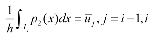
To simplify matters, the computational mesh is divided into several cells , each with a uniform size and associated cell centers are . Utilizing the intervals Ii as our control volumes, we can reformulate the semi-discretization of Eq. (1) as follows:
where is the cell average. We represent Eq. (2) with the following conservative formulation:
where is the numerical approximation to the cell average , and the non-viscous numerical flux is defined by cedures narrated latter. A sixth order scheme [38] is adopted for the viscous numerical flux .
If we can reconstruct , then Eq. (3) is the r-th order approximation to Eq. (2). Now we provide a detailed explanation of the reconstruction procedure of to approximate up to third-order and fifth-order, respectively. Additionally, the reconstruction procedure for is symmetrically mirrored with respect to of that for .
Step 1. Select the larger stencil for the third-order case (or for the fifth-order case). Then, a quartic polynomial is derived from the cell averages of is obtained by ensuring
Step 2. Then, select two smaller stencils and . Subsequently, two linear polynomials based on the cell averages of and are obtained by requiring
and
Note that Eq. (7) holds for any choice of the linear weights ,, with . In order to ensure the numerical stability of spatial discretization, we require these linear weights to be positive numbers and satisfy .
Step 4. Compute the smoothness indicators to assess the smoothness of the functions within the target cell . The smaller is, the smoother the polynomial is on the target grid . The computation of these smoothness indicators follows the same methodology outlined in [18,28,29]:
where r=2 (or r=4 ) for r=1 and for . The associated explicit expressions are
or
and
Step 5. Calculate the nonlinear weights using the linear weights and smoothness indicators. Specifically, we employ τ, defined as the absolute difference between β1, β2, and β3. Notably, this definition differs from the formula outlined in [30,31,32] due to variations in the reconstruction stencils. The expression for τ was initially introduced in [22] for the finite difference approach and subsequently adopted in [29]:
Then the non-linear weights are expressed as
where, ε represents a small positive value introduced to prevent the denominator of Eq. (14) from becoming zero. Therefore, if , then within the smooth region , where the nonlinear weights are essentially consistent with the linear weights, the WENO scheme can achieve third-order or fifth-order numerical accuracy. In this study, the value of ε is set to .
Step 6. Substituting the linear weights in Eq. (7) with the nonlinear weights specified in Eq. (14), we derive the updated reconstruction formulation for the conservative values u(x, t) at the point within the target cell , as follows:
Step 7. The semi-discretization scheme presented in Eq. (3) undergoes temporal discretization using a third-order TVD Runge-Kutta method [33]:
2.2. WENO-ZQ Scheme in Two Dimensions
Next we consider the two-dimensional N-S equation:
To simplify matters, the grid meshes are uniformly partitioned into cells, with each cell having sizes represented by and cell centers denoted by . Two dimensional cells are labeled as and the semi-discrete finite volume scheme is defined as follows:
We approximate Eq. (18) through a conservative formulation as follows:
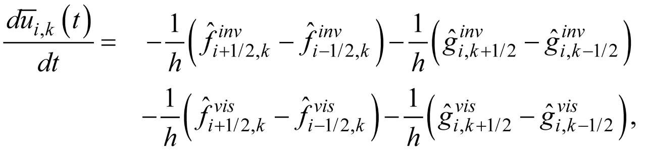
where the numerical fluxes and are defined as
to approximate and , respectively. , and
represent the weights and nodes of a three-point Gaussian within the cell , respectively. Here and denote the fifth-order approximations of and , respectively, which will be reconstructed by WENO procedures. The numerical fluxes and are determined as one-dimensional monotone fluxes.
Now, employing a dimension-by-dimension approach, we elucidate the reconstruction process for point values from cell averages .
- In the x-direction, utilizing , we execute the WENO reconstruction procedure described earlier for the one-dimensional case to reconstruct
- In the y-direction, utilizing , we apply the WENO reconstruction method outlined above for the one-dimensional scenario to reconstruct the point values . Once again, we calculate the nonlinear weights only once for all three Gauss points in the y-direction. In contrast, for classical WENO reconstruction, nonlinear weights must be computed at least three times. Additionally, negative linear weights occur at Gauss point σ2 = 0 in classical WENO reconstruction, necessitating the application of techniques to address negative linear weights in WENO reconstruction [34].
Reconstructing the point values from cell averages is similar to that for . Notably, in this step, the intermediate results should be a point value in the direction, but the cell averages in the x direction.
After the abovementioned steps, the semi-discretization scheme Eq. (19) is temporally discretized using a third-order TVD Runge-Kutta method Eq. (16).
Extending the third-order and fifth-order finite volume WENO-ZQ schemes to the three-dimensional scenario follows a dimension-by-dimension approach, akin to the two-dimensional counterpart. Similar to the two-dimensional case, it becomes evident that the novel third-order and fifth-order finite volume WENO-ZQ schemes outlined in this study surpass the classical same-order finite volume WENO-JS schemes in [28]. This superiority stems from the ability to employ identical linear weights across various quadrature points along the boundaries of the target cell, thereby significantly reducing the reconstruction process's computational burden.
2.3. All Strategies in the Framework
In this paper, all strategies are developed based on a three-dimensional, viscous, unsteady, compressible, finite volume, and RANS/LES CFD framework of the NUAA-Turbo solver using the multi-block structured grid topology. To handle both low- and high-speed flows for aerodynamic analysis, a global preconditioning technique [35] is adopted. The governing equations are expressed in the form of a conservative flux formula using primitive variables, as shown in Eq. (21). The system of nonlinear equations is solved using Newton’s implicit method [35] or a third-order TVD Runge-Kutta explicit method [33]. Dual time stepping is implemented for time accuracy in the implicit solver.
The Wall-Adapting Local Eddy-viscosity (WALE) subgrid-scale model, proposed by [36], recovers the proper y3 near-wall scaling for the eddy viscosity without requiring dynamic procedure and is adopted to simulate the LES numerical tests in this paper. The WALE model formula is as follows:
The AUSM+−up flux splitting scheme [37] is employed in this paper to calculate the numerical inviscid flux as:
where uL and uR are the reconstructed left and right valuables on the face of the control volume . So, in this framework, LES simulation uses the third-order Runge-Kutta explicit method [33], AUSM+−up flux splitting scheme [37] coupled with the fifth-order WENO schemes reconstruct interface valuables, and a sixth-order scheme [38] for the viscous flux.
2.4. Spectral Properties of WENO-ZQ Scheme
Taylor series analysis and Fourier spectrum analysis are common techniques to study the accuracy, stability, dissipation, and dispersion of constructed numerical schemes [39]. Taylor series analysis is usually used to analyze the accuracy of linear scheme, while Fourier spectrum analysis is used to analyze the dissipation and dispersion properties of numerical schemes and only applies to linear equations. Therefore, when discussing the accuracy and spectral characteristics of nonlinear schemes (such as the WENO scheme for capturing shock waves or contact discontinuities), one usually refers to the accuracy and spectral characteristics of the linear part of the nonlinear scheme. In this paper, the WENO scheme's spectral characteristics are analyzed using the numerical method for solving the approximate dispersion relation (ADR) proposed by Pirozzoli [40]. By solving the periodic solution of the linear wave equation and the discrete Fourier transform, the modified wavenumber of the nonlinear scheme can be approximately obtained, which can be used to analyze the dissipation and dispersion characteristics of the nonlinear scheme.
Zhu and Qiu [22] choose three types of the linear weights which are (1) , and ; (2) , , and ; (3) , , and in the numerical accuracy cases to illustrate the random choice of the linear weights would not pollute the optimal order of accuracy. In this section, these types of the linear weights are selected to show the spectral characteristics of the fifth-order WENO-ZQ (WENO-ZQ5) scheme in Figure 1. Although the linear weights are selected differently, they show the same trend, and the latter two curves are very close. Through verification, it is found that when the linear weight of the largest stencil is further reduced, it is also very close to the 3-curve. The following WENO-ZQ schemes adopt the first type of the linear weights as , , and , unless specified otherwise.
Figure 2 shows that the third-order WENO-ZQ (WENO-ZQ3) scheme has better spectral properties than the third-order WENO-JS (WENO-JS3) scheme. The spectral property of the third-order MUSCL scheme with a mind limiter is also presented in the figure. The dissipation and dispersion of the WENO-ZQ3 scheme are less than those of the MUSCL scheme. However, the MUSCL scheme’s dispersion is higher than that of the spectral method, which indicates that the amplitude of the calculated wave is higher than the theoretical value, which may lead to a higher prediction efficiency than the actual value in the internal flow. The dispersion of the WENO-ZQ5 scheme is better than that of the fifth-order WENO-JS (WENO-JS5) scheme in the whole wave number range. Only in the range of φ < 0.95, the dissipation is less than that of the WENO-JS5 scheme, which indicates that it can better resolve the high-frequency waves than the WENO-JS5 scheme.
2.5. Calibration the Coefficient Cw of the WALE Model
Although the WENO-ZQ scheme has good spectral characteristics, as a three-dimensional viscous CFD solver, it is necessary to consider the dissipation characteristics of mutually coupled systems, such as flux method, interface value reconstruction, viscous flux calculation method, turbulence model, etc. Decaying homogenous isotropic turbulence (DHIT) is a simple and important test case used to calibrate numerous CFD solvers. Here, we adopt the AUSM-up flux splitting scheme, the WENO-ZQ scheme to reconstruct interface values, the second-order central difference to calculate the viscous flux, and the WALE sub-grid model to calibrate Cw in WALE model with energy spectra of the experimental measurements by Comte-Bellot and Corrsin [41]. The measurements have been made dimensionless, so the computational domain is the unit box. The field is initialized at the physical times 42M/Uo in the experiment. M = 0.0508m and Uo = 10m/s are the size of the turbulence-generating mesh and free stream velocity, respectively. The detailed generation method of the initial flow field is discussed by Rozema et al. [42]. The grid cell distribution is 643, and periodic boundary conditions are applied in all directions. Many Cw are selected to calculate and compare with the experiment. Finally, Cw = 0.45, which agrees with the experiment results, is selected to present here. Figure 4 shows the energy spectrum investigated with different WENO schemes at the two subsequent physical times (98 and 171 M/Uo) computed using the WALE model and the CBC experiment [41]. The calculated results are in good agreement with the experimental data.
2.6. Unsteady Convergence Compared with WENO-JS Scheme
The three-dimensional viscous Taylor-Green vortex (TGV) [43] is a typical benchmark case in fluid mechanics, commonly used to assess the capabilities of viscous flow solvers in simulating vortex structure evolution, turbulent transition, and kinetic energy dissipation. Due to its simple initial and boundary conditions and known analytical solutions, it can be employed to evaluate the accuracy and convergence of numerical methods. The physical domain is a cube with a side length of 2πL, which contains the vorticity of the initial flow field with a smooth distribution. It is solved with the following initial conditions to present the convergence of the unsteady solution by various high-order schemes.
Detailed flow and initial conditions used here were specified in [43]. The Reynolds number of the flow is defined as and equals 1600. In this field, kinetic energy is transferred from the large scale down to the smaller scale until it reaches a sufficiently small length scale. Finally, it dissipates into internal energy under physical viscosity. The largest dissipation rate occurs at . The purpose here is to evaluate the convergence property of the schemes. This paper investigates the evolution of the Taylor-Green vortex with time using four different mesh sizes, 32×32×32, 64×64×64, 128×128×128, and 256×256×256, under different WENO schemes. Coherent structures in the field are observed employing a Q-criterion, with iso-surfaces set at , and velocity magnitude colors the iso-surfaces.
Figure 5, Figure 6, Figure 7 and Figure 8 illustrate the Taylor-Green vortex flows computed with different WENO schemes for comparative analysis. Computational results show that the new WENO-ZQ schemes can capture more turbulence structures than those of the same order WENO-JS schemes across identical meshes. Moreover, the computed flows demonstrate favorable symmetry in the vortex structures, suggesting that the schemes effectively preserve the flow field's symmetry.
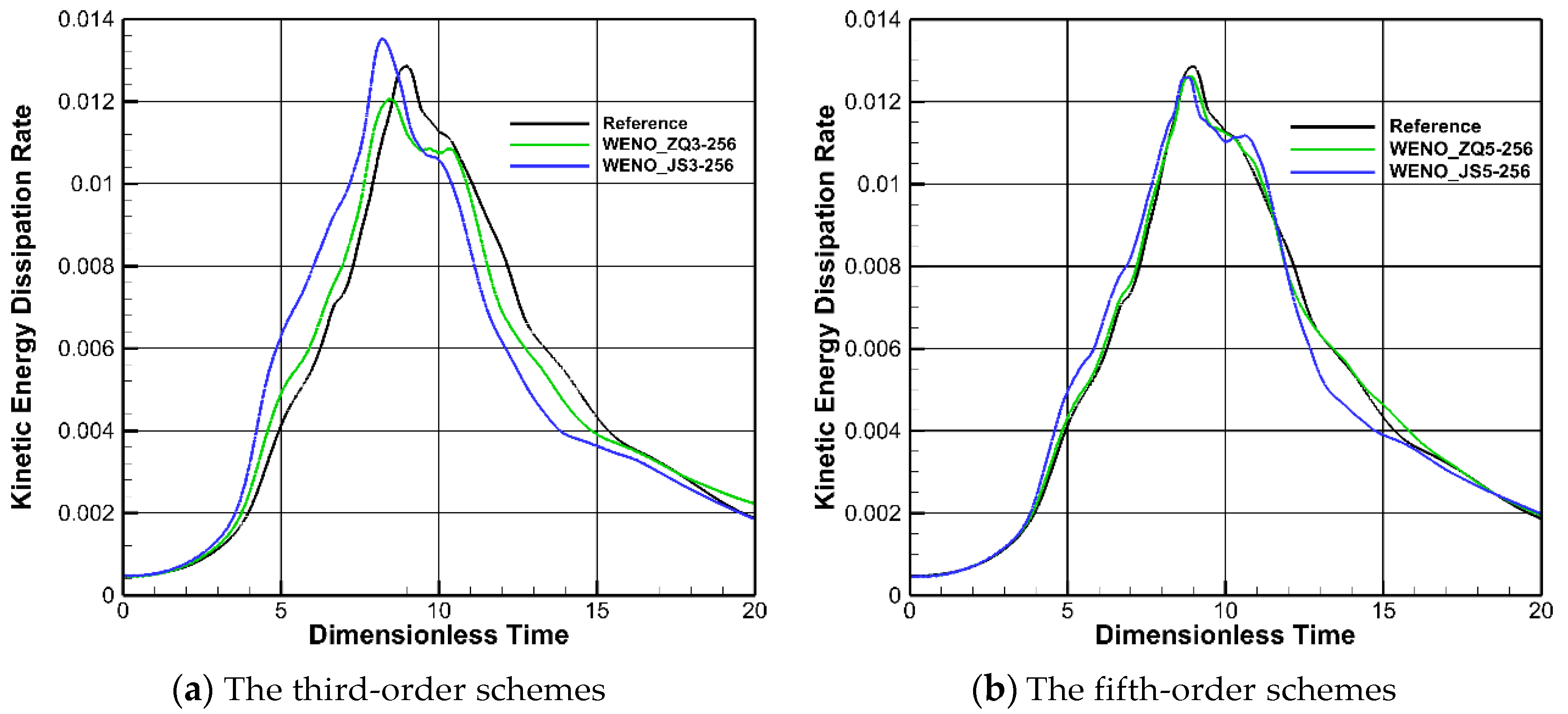
The evolution of kinetic energy and its dissipation rate is contrasted with the reference solution acquired from the pseudo-spectral code [44]. The evolution of kinetic energy calculated on different meshes is shown in Fig. 9. The results of the WENO-ZQ scheme on 32×32×32 cells are similar to that of the WENO-JS scheme on 64×64×64 cells. It is shown that the convergence rate of the WENO-ZQ scheme is faster than that of the WENO-JS scheme. The numerical results show that these new high-order finite volume WENO schemes reduce the computational cost and capture more details of flow physics than classical WENO-JS schemes [18]. The kinetic energy dissipation rates calculated using different schemes on 256×256×256 cells are shown in Fig. 10. It can be observed from the figure that the WENO-ZQ scheme is closer to the reference solution.
Figure 10.
Evolution of kinetic energy dissipation rates by various WENO schemes
3. Numerical Tests of Turbomachinery Flow
In order to further investigate the properties of the new WENO schemes developed in the LES CFD framework in this paper, some numerical tests of turbomachinery flow containing various physical phenomena, such as transition, separation-induced transition, the wake of the turbine, and the interaction between shock wave and turbulence boundary layer, are presented in this section.
3.1. Turbulent Boundary Layer Simulation
Generating three-dimensional, time-dependent turbulent inflow data is critical in conducting large eddy simulations (LES) of complex spatially developing turbulent boundary layers (TBL). Obtained TBL with specified boundary layer thickness (δ) and friction velocity (uτ) is the key to the study of shock wave and turbulent boundary layers interaction (SWTBI). In this paper, the recycling and rescaling method (RRM) proposed by Lund, Wu, and Squires [45] and further developed by Urbin and Knight [46] is adopted to generate the inflow data for TBL. The WENO schemes are used to simulate this case, and the results are compared with those simulated by Dawson et al. [47].
Figure 11 shows the computational domain. To avoid confusion, we will refer to the x, y, and z directions as streamwise, wall-normal, and spanwise unless specified otherwise. The mesh contains 310×111×119 cells in the x, y, and z directions. The grid resolution is Δx+=4.05, Δy+= 0.23, and Δz+=2.64 in the wall. The upper and right boundaries of the computational domain are set as supersonic outlet boundary conditions. The non-slip isothermal wall condition is implemented in the button wall, and the wall temperature is 307K. Periodic boundary conditions are used in the z-direction. The boundary conditions of inlet turbulence are given dynamically by the RRM. Table 1 contains the main parameters of the turbulent boundary layer on the incoming plane.
In order to compare with different schemes, 200 dimensionless time flow field information are analyzed. Figure 12 shows the mean velocity profiles by Van Driest transformation [51] at the recycled plane, is dimensionless by uτ. As can be seen from the figure, the distribution calculated by the WENO-JS5 and WENO-ZQ5 schemes in the viscous sublayer and log layer coincides with the classical law of the wall. The distribution of Reynolds stress normal to the wall of recycling plane is compared with Dawson’s LES results [47]. As shown in Figure 13, the distribution obtained by those schemes is basically the same. Coherent structures are also visualized by Q-criterion () and the iso-surfaces are colored by local Mach number at the same time in Figure 14, and the WENO-ZQ5 scheme can capture richer flow structure than that of the WENO-JS5 scheme. The comparison of velocity profile, Reynolds stress, and coherent structures shows that this paper's WENO-ZQ5 and WENO-JS5 schemes can generate a reasonable and effective turbulent boundary layer.
3.2. Shock Wave/Turbulent Boundary Layer Interaction (SWTBLI)
The SWTBLI represents a critical aerodynamic and thermodynamic process in the supersonic inlet flow. It can lead to significant alterations in heat transfer in the external flow and produce unsteady pressure loads, potentially shortening the lifespan of structures. Internally, it may trigger large-scale, unsteady separated flows, increasing total pressure loss and causing flow distortion that can lead to engine surge. The compression ramp model, despite its simplicity, captures essential SWTBLI phenomena such as boundary layer separation, reattachment, and turbulence enhancement due to inverse pressure gradients [48]. The highly three-dimensional flow field features intricate multi-scale interactions, making it an ideal test case for validating CFD methods.
Figure 15 depicts the schematic of the computational domain, where the inlet boundary layer thickness (δ) measures 6.7mm. This domain comprises two main sections: the flat plane computation domain, referred to as the auxiliary computation domain, and the 24° compression ramp computation domain, denoted as the primary computation domain [48]. Within the auxiliary computation domain, the RRM model generates the turbulent boundary layer, which subsequently serves as the inlet boundary condition for the primary computation domain. The coordinate system's origin is situated at the ramp, with both upstream and downstream lengths spanning 7.73δ, a spanwise width of 2.15δ, and a normal height along the wall measuring 5.23δ. The number of grid points in three directions is 505×89×112, corresponding to the streamwise, the spanwise, and the normal directions, respectively. Refined mesh is implemented along the normal direction (y) near the wall to ensure that the height of the first cell layer satisfies Δy+< 0.5. The flow field within the recycled plane of the auxiliary computation domain is extracted to serve as the inlet boundary conditions for the primary computation.
Figure 16 depicts the distribution of the average wall pressure () and the average skin friction coefficient (Cf) along the streamwise direction within the primary computation domain. Additionally, experimental data by Bookey et al. [48] and the direct numerical simulation (DNS) results by Wu et al. [49] are presented. From the figure, it can be observed that the averaged separation point in the ramp flow occurs at , and the reattachment point is located at , where the skin friction coefficient Cf equals zero. Both are in good agreement with the experimental results.
Figure 17 shows the instantaneous flow structure within the primary computation domain. It illustrates the turbulent boundary layer’s quasi-ordered structure using the Q-criterion and colors it based on streamwise velocity. The semi-transparent gray surface in the figure represents the dimensionless pressure iso-surface (), which depicts the three-dimensional structure of the separation shock wave. It is evident from the figure that the flow field within the interaction region exhibits pronounced three-dimensional characteristics. As large vortex structures traverse the root of the shock wave, they undergo fragmentation at the ramp due to intensified turbulent fluctuations. Concurrently, deformation of the shock wave occurs at its root, with surface wrinkling becoming evident along the spanwise direction. It is observed that the shock wave maintains typical two-dimensional structural features when situated away from the interaction region.
3.3. Pak B Low Pressure Turbine Cascade
The boundary layer transition from laminar to turbulent flow is a very important and complex problem in fluid mechanics. Understanding the physical mechanisms of boundary layer transition is of great significance in studying the formation mechanism of turbulence, and the prediction and control of transition is also of great application value in engineering.
Due to the working environment of a low-pressure turbine, the boundary layer state of the suction surface is greatly affected by the transition. The ability to accurately predict the separation of laminar flow and the transition of the boundary layer is essential for the design of high-load, low-loss, low-pressure turbines. However, the transition is caused by non-linear instability and requires a higher accuracy method to capture small-scale vortex.
The load factor Zweifiel Coefficient of Pak B blade profile is selected to test the WENO-ZQ5 scheme, which is a typical high-load turbine blade profile. It comes from the middle section of a Pratt and Whitney unmanned aerial vehicle's low-pressure blade; the main parameters are presented in Table 2. The specific blade profile data are from reference [52], and the experimental data are from reference[53]. The free stream turbulence intensity (FSTI) is 0.08% and the Reynolds number based on the exit velocity and the suction surface length is 100,000 from experiments.
Only 30 grid points are given in the blade height direction. The length between the inlet and the leading edge of the cascade is about one time the chord length, and the outlet to the trailing edge is about two times the chord length. 330 nodes are arranged on the suction surface. The first grid near the wall is Δy+ = 0.3. The grid growth rate along the wall is 1.1, and the total number of grids is 4.07 million.
Figure 18 shows the calculated blade surface static pressure coefficient Cp. The numerical simulation results of the pressure surface of the blade are in good agreement with the experimental data, and the location and size of the separation bubble on the pressure surface are accurately simulated. There is a pressure platform at on the suction surface of the blade, and the separation occurs on the suction surface and then reattachment. However, there is a slight difference in the separation area on the suction surface compared with the experiment. At the same time, the velocity distributions at different suction surface positions are shown, which are 50%, 60%, 70%, 75%, 80%, 85%, and 90% of the axial chord length, respectively. It can be seen that the numerical simulation results are consistent with the experimental values, and there is a slight deviation between the numerical simulation results and the experimental values at the reattachment point. The coherent structures of the suction surface of Pak B are shown in Figure 19. Generally speaking, the method used in this paper can accurately predict the separation and the transition caused by separation in the low-pressure turbine.
4. Conclusions
This paper implements a new type of finite volume high-order WENO scheme into the NUAA-Turbo software for solving three-dimensional Navier-Stokes equations on structured meshes. The key advantages of this WENO scheme are their simplicity and ability to obtain optimal high-order accuracy by applying a series of unequal-sized spatial stencils in reconstructions. This new finite volume WENO methodology utilizes information from a combination of spatial stencils, including one five-cell stencil and two smaller two-cell stencils in each direction. Linear weights are artificially assigned to ensure conservation, while smoothness indicators are computed, and nonlinear weights are redefined accordingly. The construction of these WENO schemes is rooted in WENO interpolation within the spatial field, followed by implementing a third-order TVD Runge-Kutta time discretization method to solve the ordinary differential equations
Compared with the classical same-order WENO-JS schemes, the new finite volume WENO schemes are very simple in the computation of problems containing various physical phenomena such as transition, separation induced transition, and the interaction between shock wave and turbulence boundary layer in the LES framework. They achieve the same level of accuracy while minimizing absolute numerical truncation errors. These high-order WENO schemes are easily applied in aero-engine internal flow simulation. Although the calculation process of classical WENO schemes is complex in practical applications or results in the appearance of instability, these new high-order finite-volume WENO schemes do not have these drawbacks at all. So, the new WENO schemes can reduce the computational cost in aerodynamic applications by using fewer grid cells, capturing more flow physics details, and improving the robustness and stability in large-scale engineering applications.
Author Contributions
For research articles with several authors, a short paragraph specifying their individual contributions must be provided. The following statements should be used “Conceptualization, S.Z. and D.Z.; methodology, S.Z. and D.Z.; software, D.Z.; validation, S.Z., H.W. and X.W.; formal analysis, X.W.; investigation, S.Z.; data curation, D.Z.; writing—original draft preparation, S.Z.; writing—review and editing, N.G.; supervision, W.H.; funding acquisition, N.G. All authors have read and agreed to the published version of the manuscript.
Funding
Please add: This research was funded by NATIONAL SCIENCE AND TECHNOLOGY, grant number Y2019-I-0018-0017.
Data Availability Statement
Not applicable.
Conflicts of Interest
The authors declare no conflicts of interest.
References
- Laskowski, G.M.; Kopriva, J.; Michelassi, V.; Shankaran, S.; Paliath, U.; Bhaskaran, R.; Wang, W.Q.; Talnikar, C.; Wang, Z.J.; Jia, F.L. Future Directions of High Fidelity CFD for Aerothermal Turbomachinery Analysis and Design. 46th AIAA Fluid Dynamics Conference, Washington, DC, U.S.A. 13-17 June 2016. [CrossRef]
- Zhang, S.; Si, T.Y.; Zhang, X.M.; Li, H.Y.; Xi, D.K.; He, W.Q.; Zhang, A.C. Research progress of skew and sweep aerodynamic technology for turbomachinery blades. J. Propul. Techno. 2021, 42, 2417–2431. (In Chinese) [Google Scholar] [CrossRef]
- Liu, Y.Z.; Zhao, W.; Zhao, Q.J.; Zhou, Q.; Xu, J.Z. Passage shock wave/boundary layer interaction control for transonic compressors using bumps. Chinese J. Aeronaut. 2022, 35, 82–97. [Google Scholar] [CrossRef]
- Wu, Y.H.; Wang, B.; Fu, Y.; Liu, J. Research progress of corner separation in axial-flow compressor. Chinese J. Aeronaut. 2017, 38, 102–123. (In Chinese) [Google Scholar] [CrossRef]
- Zhou, Q.H.; Zhao, W.; Sui, X.M.; Zhao, Q.J.; Xu, J.Z. A shock loss reduction method using a concave suction side profile for a zero inlet swirl turbine rotor. J. Turbomach. 2022, 144, 111010. [Google Scholar] [CrossRef]
- Li, J.; Hu, J.; Wang, Z.Q.; Tu, B.F. Investigation of corner separation in axial compressor stator using DDES. J. Aerosp. Power 2021, 36, 687–700. (In Chinese) [Google Scholar] [CrossRef]
- Li, X.; Zheng, Q.; Chi, Z.D.; Wang, S.M.; Zhou, Z.T.; Jiang, B. Research on the influence of spanwise cross-flow on the boundary layer transition of compressor cascade. Phys. Fluids 2024, 36, 014127. [Google Scholar] [CrossRef]
- Sandberg, R.D.; Michelassi, V. The current state of high-fidelity simulations for main gas path turbomachinery components and their industrial impact. Flow Turbul. Combust. 2019, 102, 797–848. [Google Scholar] [CrossRef]
- Van Ingen J, L. The en Method for Transition Prediction, Historical Review of Work at TU Delft . In Proceedings of the 38th Fluid Dynamics Conference and Exhibit, Seattle, U.S.A., 23-26 June 2008. [Google Scholar] [CrossRef]
- Gourdain, N. Prediction of the unsteady turbulent flow in an axial compressor stage. Part 1: Comparison of unsteady RANS and LES with experiments. Comput. Fluids 2015, 106, 119–129. [Google Scholar] [CrossRef]
- Gourdain, N. Prediction of the unsteady turbulent flow in an axial compressor stage. Part 2: Analysis of unsteady RANS and LES data. Comput. Fluids 2015, 106, 67–78. [Google Scholar] [CrossRef]
- Miki, K.; Ameri, A. Improved prediction of losses with large eddy simulation in a low-pressure turbine. J. Turbomach. 2022, 144, 071002. [Google Scholar] [CrossRef]
- Harten, A. High resolution schemes for hyperbolic conservation laws. J. Comput. Phys. 1983, 49, 357–393. [Google Scholar] [CrossRef]
- Harten, A.; Engquist, B.; Osher, S.; Chakravarthy, S.R. Uniformly high order essentially non-oscillatory schemes, Ⅲ. J. Comput. Phys. 1987, 71, 231–303. [Google Scholar] [CrossRef]
- Harten, A. Preliminary results on the extension of ENO schemes to two-dimensional problems. Lect. Notes Math., 1987, 1270, 23–40. [Google Scholar] [CrossRef]
- Godunov, S.K.; Bohachevsky, I. A finite-difference scheme for the numerical computation of discontinuous solutions of the equations of fluid dynamics. Matematicheskii Sbornik, 1959, 47, 271–306. [Google Scholar]
- Liu, X.D.; Osher, S.; Chan, T. Weighted essentially non-oscillatory schemes. J. Comput. Phys. 1994, 115, 200–212. [Google Scholar] [CrossRef]
- Jiang, G.S.; Shu, C.W. Efficient implementation of weighted ENO schemes. J. Comput. Phys. 1996, 126, 202–228. [Google Scholar] [CrossRef]
- Wang, S.Y.; Deng, X.G.; Dong, Y.D.; Wang, D.F.; Cai, J.H. High-order numerical methods for engineering turbulence simulation. Acta Aeronaut. Astronaut. Sin. 2023, 44, 528728. (In Chinese) [Google Scholar] [CrossRef]
- Levy, D.; Puppo, G.; Russo, G. Central WENO schemes for hyperbolic systems of conservation laws. Esaim-Math. Model Num. 1999, 33, 547–571. [Google Scholar] [CrossRef]
- Levy, D.; Puppo, G.; Russo, G. Compact central WENO schemes for multidimensional conservation laws. SIAM J. Sci. Comput. 2000, 22, 656–672. [Google Scholar] [CrossRef]
- Zhu, J.; Qiu, J.X. A new fifth order finite difference WENO scheme for solving hyperbolic conservation laws. J Comput Phys. 2016, 318, 110–121. [Google Scholar] [CrossRef]
- Zhu J, Qiu J. A new type of finite volume WENO schemes for hyperbolic conservation laws. J. Sci. Comput. 2017, 1–22. [Google Scholar] [CrossRef]
- Zhong, D.D.; Sheng, C.H. A new method towards high-order WENO schemes on structured and unstructured grids. Comput. Fluids 2020, 200, 104453. [Google Scholar] [CrossRef]
- Sheng, C.H. Improving predictions of transitional and separated flows using RANS modeling. Aerosp. Sci. Technol. 2020, 106, 106067. [Google Scholar] [CrossRef]
- Zhao, Z.; Zhu, J.; Chen, Y.B.; Qiu, J.X. A new hybrid WENO scheme for hyperbolic conservation laws. Comput. Fluids 2019, 179, 422–436. [Google Scholar] [CrossRef]
- Zhu, J.; Qiu, J. A new type of modified WENO schemes for solving hyperbolic conservation laws. SIAM J. Sci. Comput. 2017, 39, A1089–A1113. [Google Scholar] [CrossRef]
- Cockburn, B., Shu, C.W.; Johnson, C.; Tadmor, E. Essentially non-oscillatory and weighted essentially non-oscillatory schemes for hyperbolic conservation laws. Advanced Numerical Approximation of Nonlinear Hyperbolic Equations. Quarteroni, A.; Springer: Berlin, Heidelberg, Germany, 1998; 1697, pp. 325-432. [CrossRef]
- Balsara, D.S.; Garain, S.; Shu, C.W. An efficient class of WENO schemes with adaptive order. J. Comput. Phys. 2016, 326, 780–804. [Google Scholar] [CrossRef]
- Borges, R.; Carmona, M.; Costa, B.; Don, W.S. An improved weighted essentially non-oscillatory scheme for hyperbolic conservation laws. J. Comput. Phys. 2008, 227, 3191–3211. [Google Scholar] [CrossRef]
- Castro, M.; Costa, B.; Don, W.S. High order weighted essentially non-oscillatory WENO-Z schemes for hyperbolic conservation laws. J. Comput. Phys. 2011, 230, 1766–1792. [Google Scholar] [CrossRef]
- Don, W.S.; Borges, R. Accuracy of the weighted essentially non-oscillatory conservative finite difference schemes. J. Comput. Phys. 2013, 250, 347–372. [Google Scholar] [CrossRef]
- Shu, C.W.; Osher, S. Efficient implementation of essentially non-oscillatory shock-capturing schemes. J. Comput. Phys. 1988, 77, 439–471. [Google Scholar] [CrossRef]
- Shi, J.; Hu, C.; Shu, C.W. A technique of treating negative weights in WENO schemes. J. Comput. Phys. 2002, 175, 108–127. [Google Scholar] [CrossRef]
- Sheng, C.H. A preconditioned method for rotating flows at arbitrary Mach number. Mod. Simul. Eng. 2011, 29. [Google Scholar] [CrossRef]
- Nicoud, F.; Frédéric, D. Subgrid-scale sNg based on the square of the velocity gradient tensor. Flow Turbul. Combust. 1999, 62, 183–200. [Google Scholar] [CrossRef]
- Liou, M.S. A sequel to AUSM, part II: AUSM+-up for all speeds. J. Comput. Phys. 2006, 214, 137–170. [Google Scholar] [CrossRef]
- Shen, Y.; Zha, G. Large eddy simulation using a new set of sixth order schemes for compressible viscous terms. J. Comput. Phys. 2010, 229, 8296–8312. [Google Scholar] [CrossRef]
- Sheng, C.H.; Zhao, Q.Y.; Zhong, D.D.; Ge, N. A Strategy to Implement High-Order WENO Schemes on Unstructured Grids. AIAA Aviation 2019 Forum, Dallas, U.S.A, 17-21 June 2019. [CrossRef]
- Pirozzoli, S. On the spectral properties of shock-capturing schemes. J. Comput. Phys. 2006, 219, 489–497. [Google Scholar] [CrossRef]
- Comte-Bellot, G.; Corrsin, S. Simple Eulerian time correlation of full-and narrow-band velocity signals in grid-generated, ‘isotropic’ turbulence. J. Fluid. Mech. 1971, 48, 273–337. [Google Scholar] [CrossRef]
- Rozema, W.; Bae, H.J.; Moin, P.; Verstappen, R. Minimum-dissipation models for large-eddy simulation. Phys. Fluids. 2015, 27, 085107. [Google Scholar] [CrossRef]
- Taylor, G.I.; Green, A.E. Mechanism of the production of small eddies from large ones. Proceedings of the Royal Society of London. Series A-Mathematical and Physical Sciences, 1937, 158, 499–521. [Google Scholar] [CrossRef]
- Van Rees, W.M.; Leonard, A.; Pullin, D.I.; Koumoutsakos, P. A comparison of vortex and pseudo-spectral methods for the simulation of periodic vortical flows at high Reynolds numbers. J. Comput. Phys. 2011, 230, 2794–2805. [Google Scholar] [CrossRef]
- Lund, T.S.; Wu, X.H.; Squires, K.D. Generation of turbulent inflow data for spatially-developing boundary layer simulations, J. Comput. Phys. 1998, 140, 233–258. [Google Scholar] [CrossRef]
- Urbin, G.; Knight, D. Large-eddy simulation of a supersonic boundary layer using an unstructured grid. AIAA Journal 2001, 39, 1288–1295. [Google Scholar] [CrossRef]
- Dawson, D.M.; Lele, S.K. Large Eddy Simulation of a Three-Dimensional Compression Ramp Shock-Turbulent Boundary Layer Interaction. 53rd AIAA Aerospace Sciences Meeting, Kissimmee, U.S.A, 05-09 January 2015. [CrossRef]
- Bookey, P.; Wyckham, C.; Smits, A. Experimental Investigations of Mach 3 Shock-Wave Turbulent Boundary Layer Interactions. 35th AIAA Fluid Dynamics Conference and Exhibit, Toronto, Canada, 06-09 June 2005. [CrossRef]
- Wu, M.; Martin, M.P. Direct numerical simulation of supersonic turbulent boundary layer over a compression ramp. AIAA Journal 2007, 45, 879–889. [Google Scholar] [CrossRef]
- Tong, F.L.; Yu, C.P.; Tang, Z.G.; Li, X.L. Numerical studies of shock wave interactions with a supersonic turbulent boundary layer in compression corner: Turning angle effects. Comput. Fluids 2017, 149, 56–69. [Google Scholar] [CrossRef]
- Huang, P.; Coleman, G.N. Van driest transformation and compressible wall-bounded flows. AIAA Journal 1994, 32, 2110–2113. [Google Scholar] [CrossRef]
- Shyne, R.J. Experimental Study of Boundary Layer Behavior in a Simulated Low-Pressure Turbine. PHD, the University of Toledo, 1998.
- Huang, J.; Corke, T.C.; Thomas, F.O. Plasma actuators for separation control of low-pressure turbine blades. AIAA Journal, 2006, 44, 51–57. [Google Scholar] [CrossRef]
Figure 1.
Spectral properties of WENO-ZQ5 scheme with three types of the linear weights.
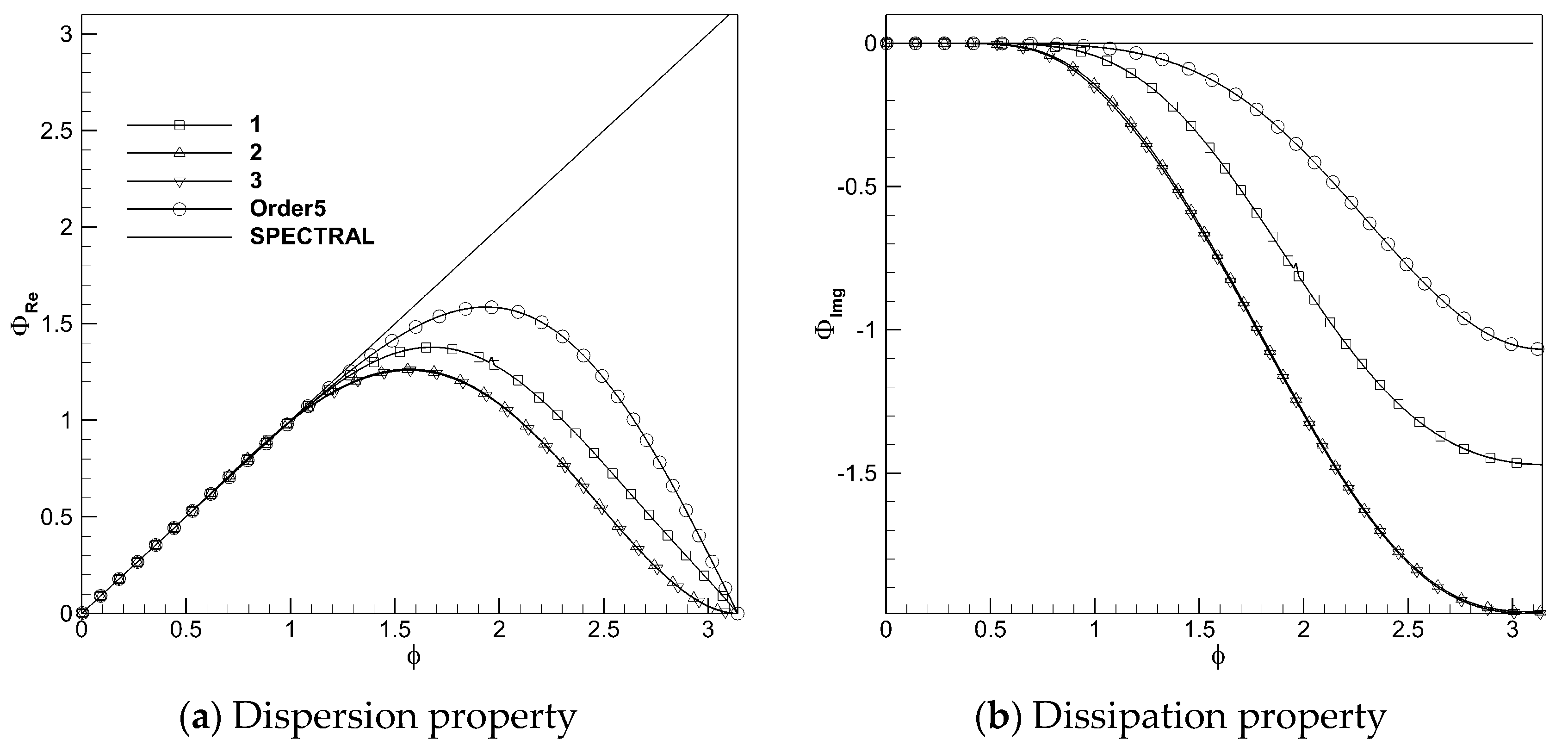
Figure 2.
Spectral properties of WENO-ZQ3 and WENO-JS3 schemes.
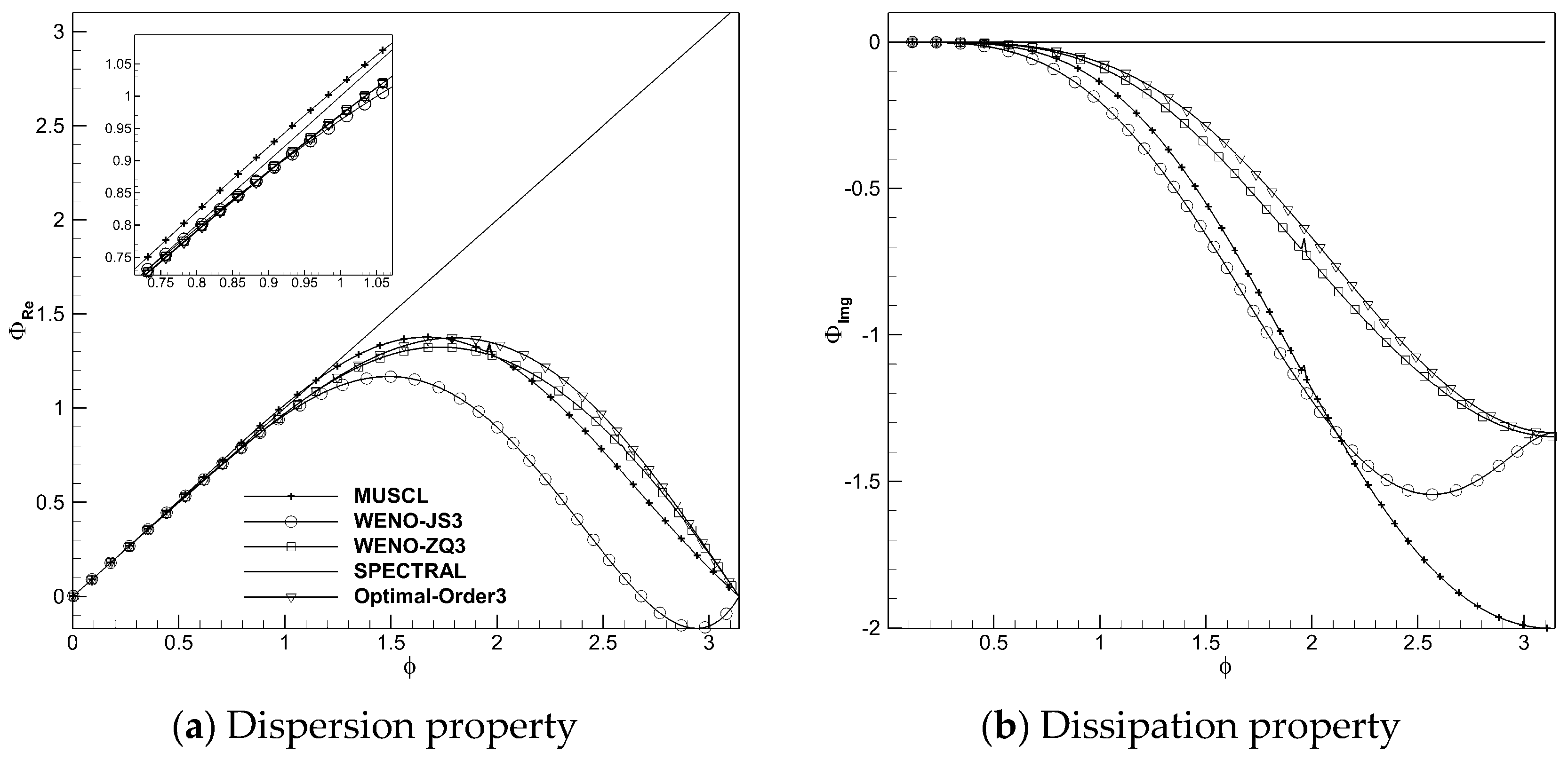
Figure 3.
Spectral properties of WENO-ZQ5 and WENO-JS5 schemes.
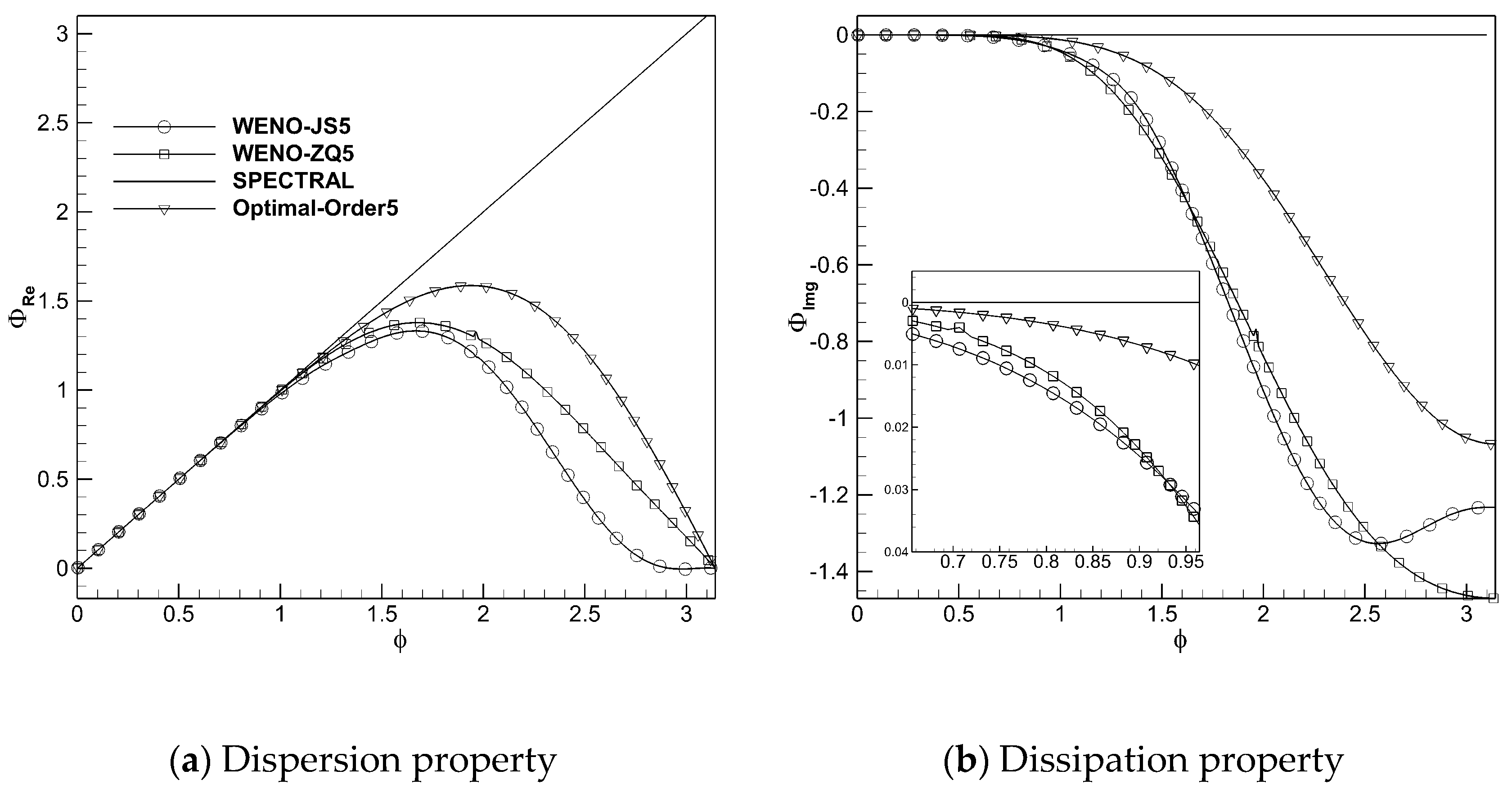
Figure 4.
Comparison of energy spectra of experiment by different schemes.
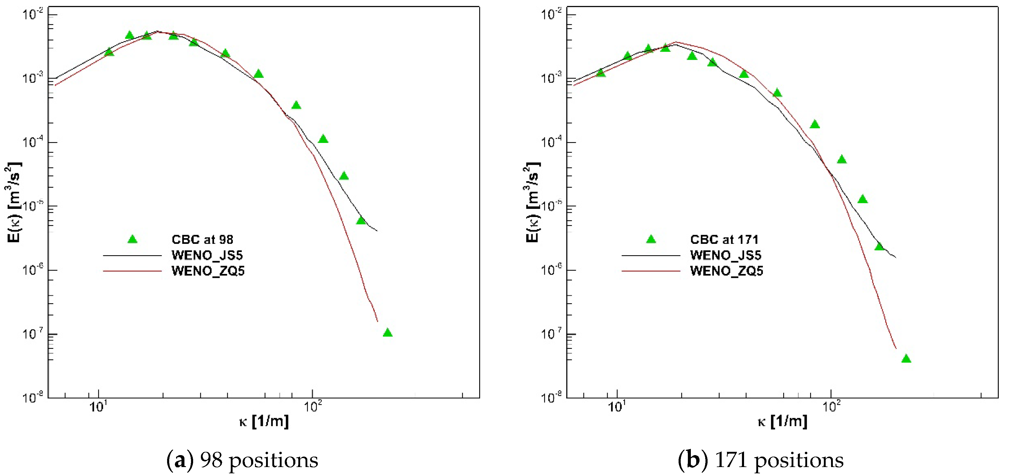
Figure 5.
Schematic of TGV problem computed by WENO-JS3 scheme on different meshes at .
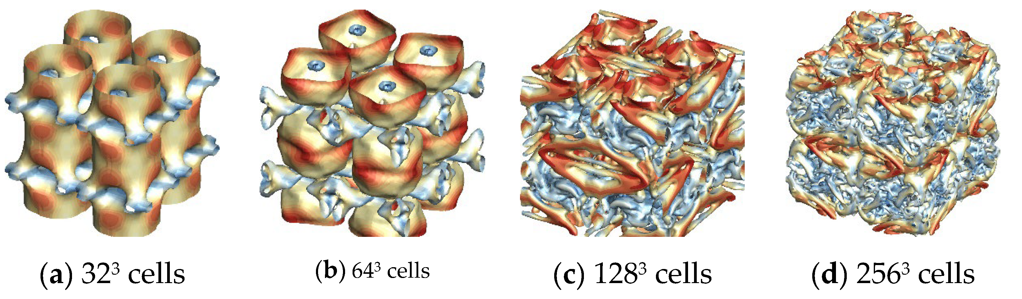
Figure 6.
Schematic of TGV problem computed by WENO-ZQ3 scheme on different meshes at .
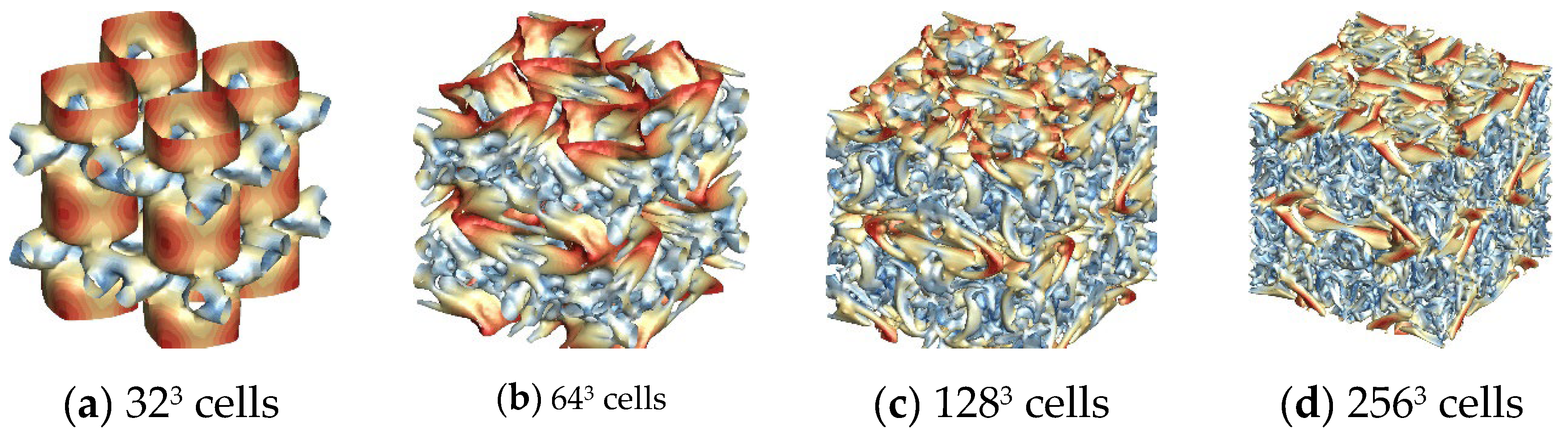
Figure 7.
Schematic of TGV problem computed by WENO-JS5 scheme on different meshes at .
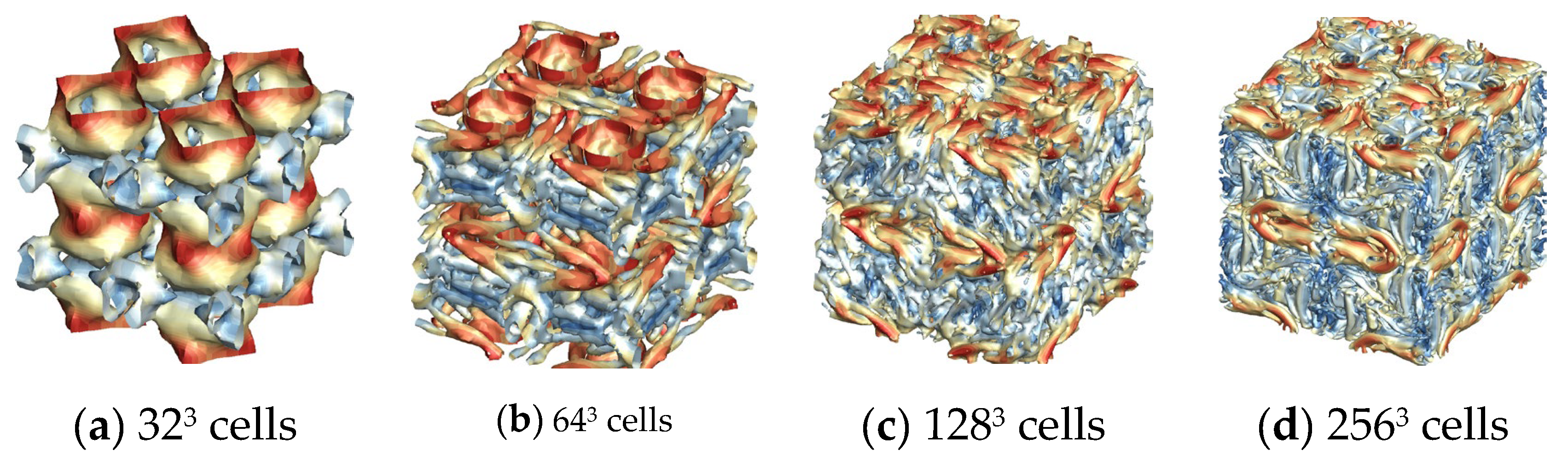
Figure 8.
Schematic of TGV problem computed by WENO-ZQ5 scheme on different meshes at .
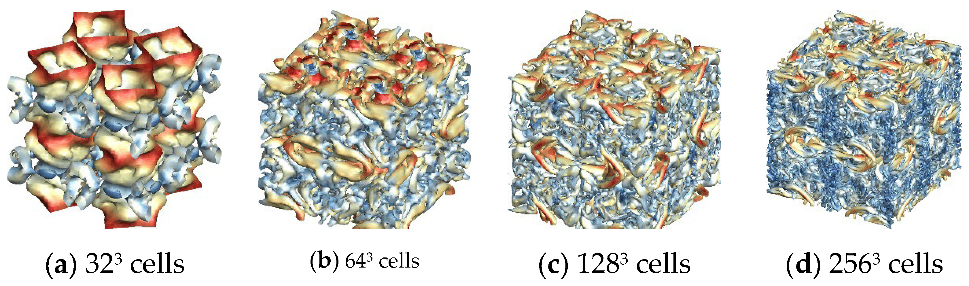
Figure 9.
Evolution of kinetic energy by various WENO schemes on different meshes.
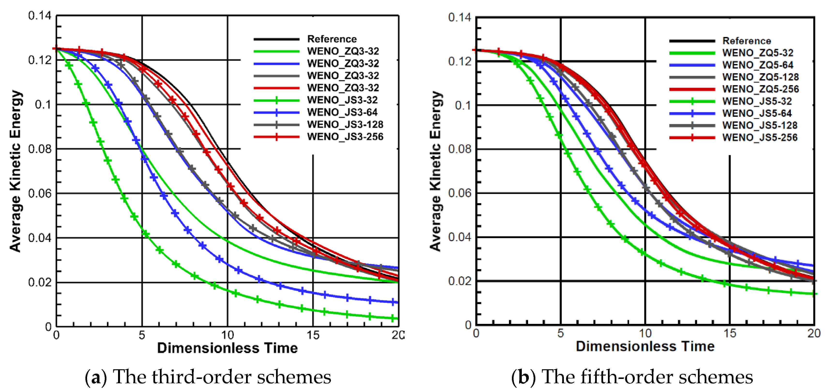
Figure 11.
Schemes follow the same formatting.
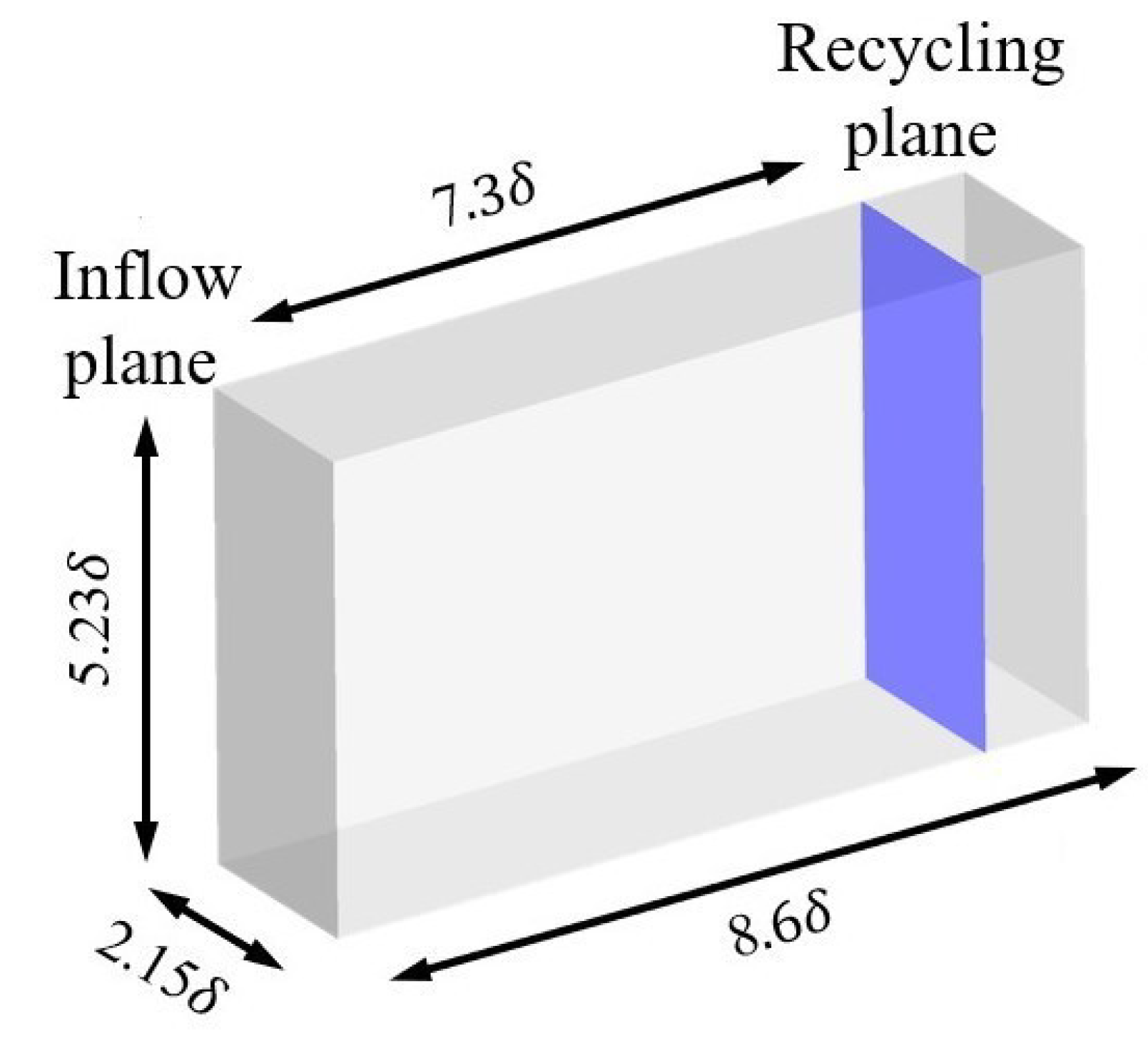
Figure 12.
Van Driest transformed mean velocity profiles.
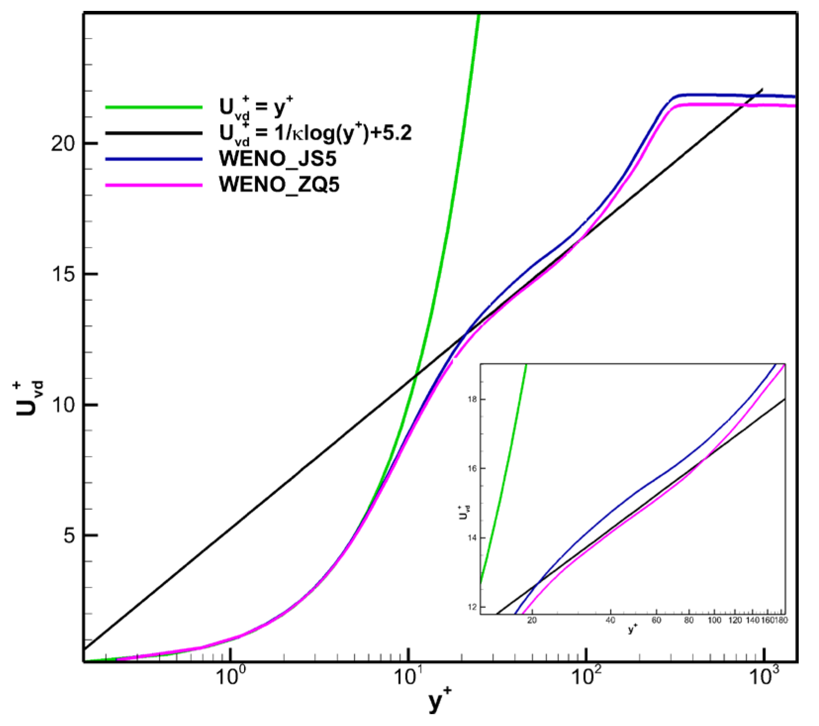
Figure 13.
Profiles of Reynolds stress at the recycling plane.
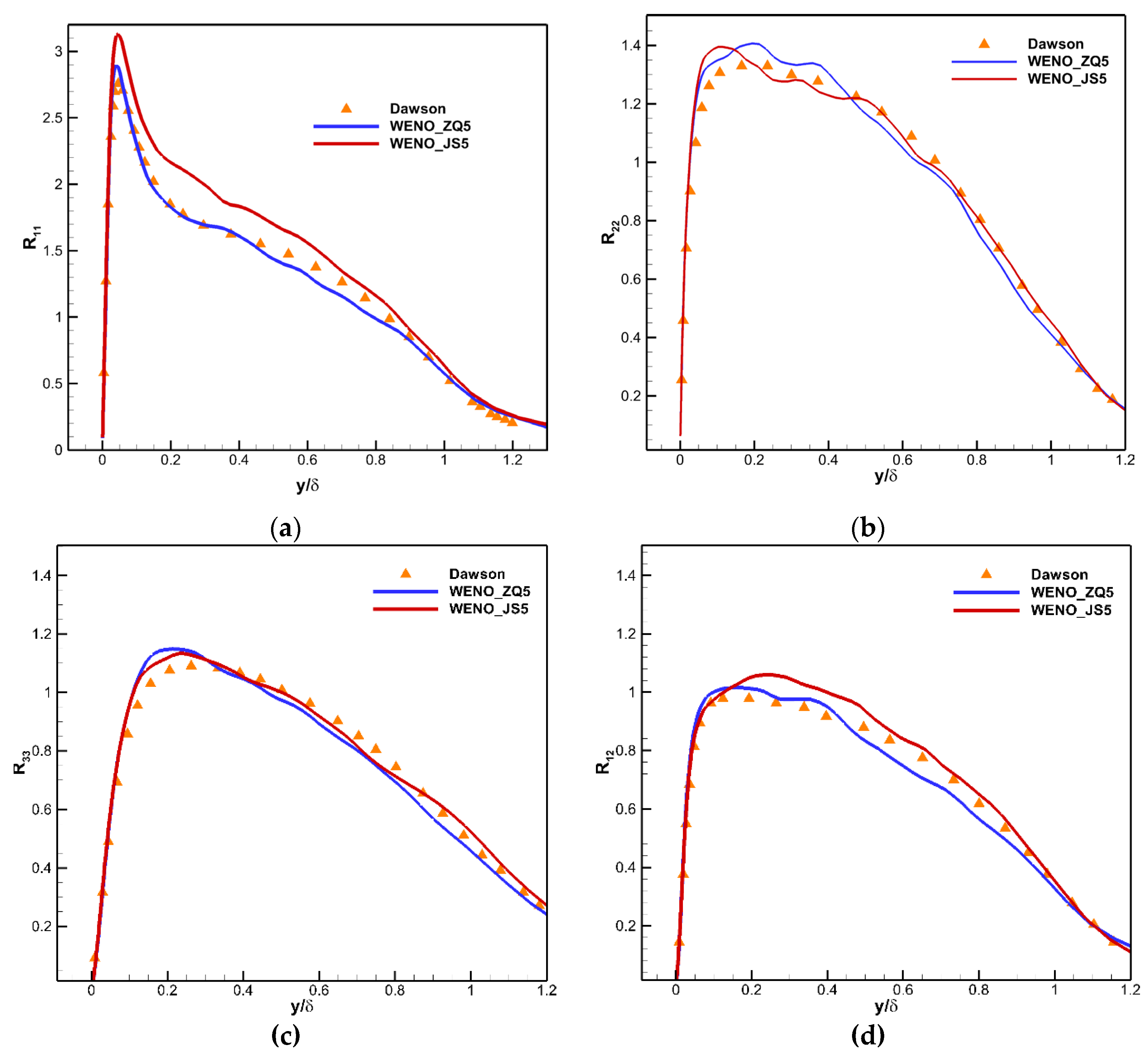
Figure 14.
Visualization of the coherent structures in supersonic turbulent boundary layer.
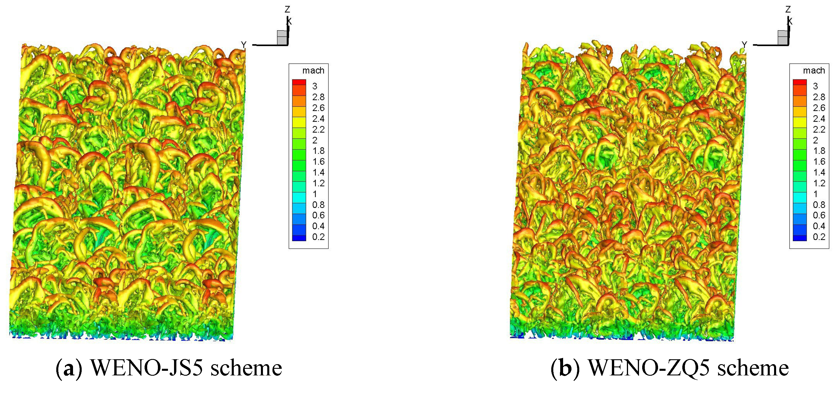
Figure 15.
Computational domain for the LES.
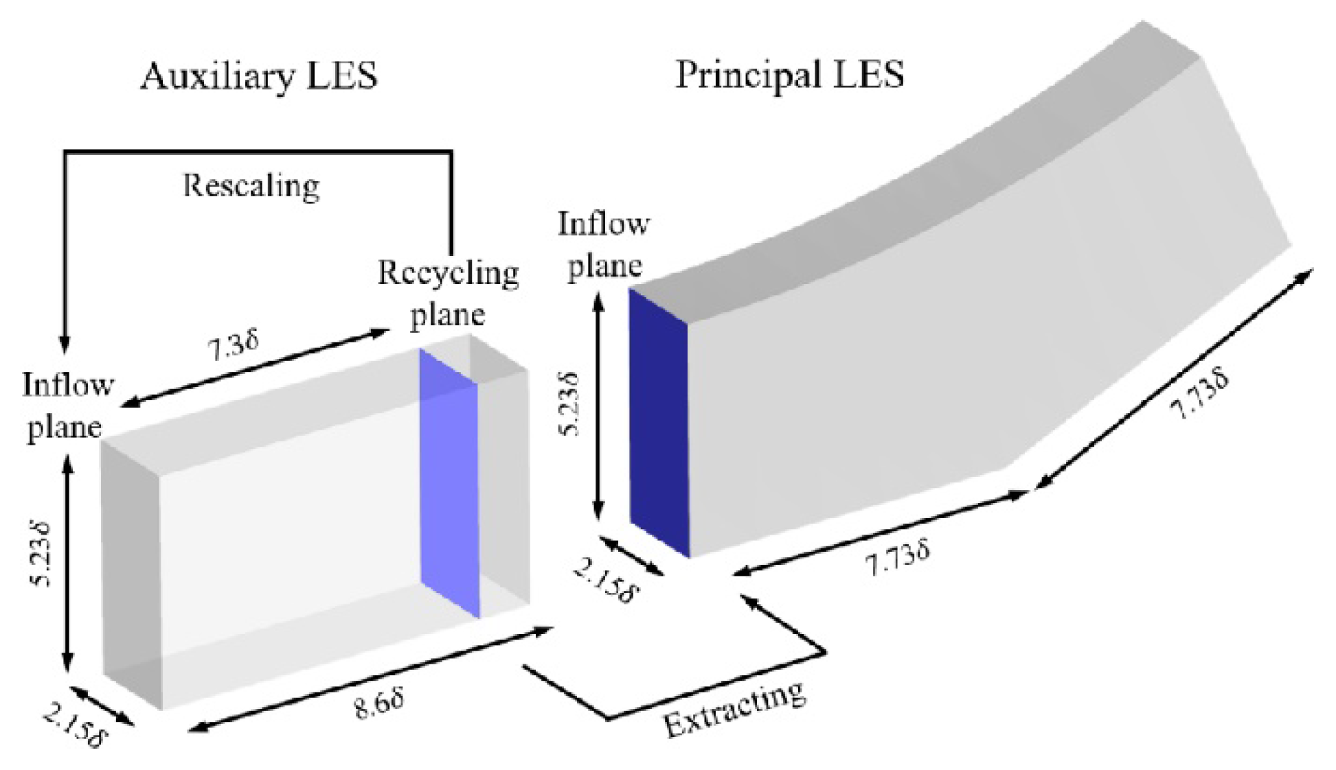
Figure 16.
Distribution of averaged wall pressure and averaged skin friction coefficient.
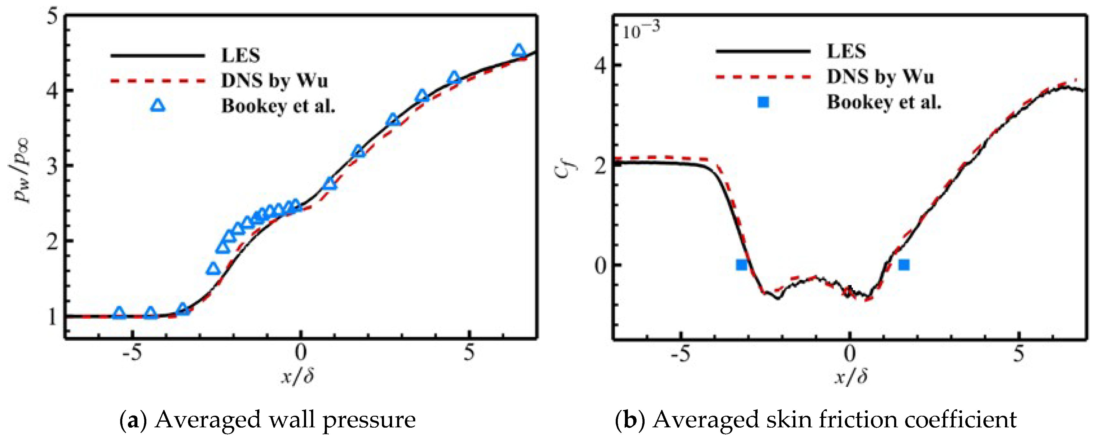
Figure 17.
Wrinkling of shock surface ().
Figure 18.
Pressure and velocity distribution of Pak B.
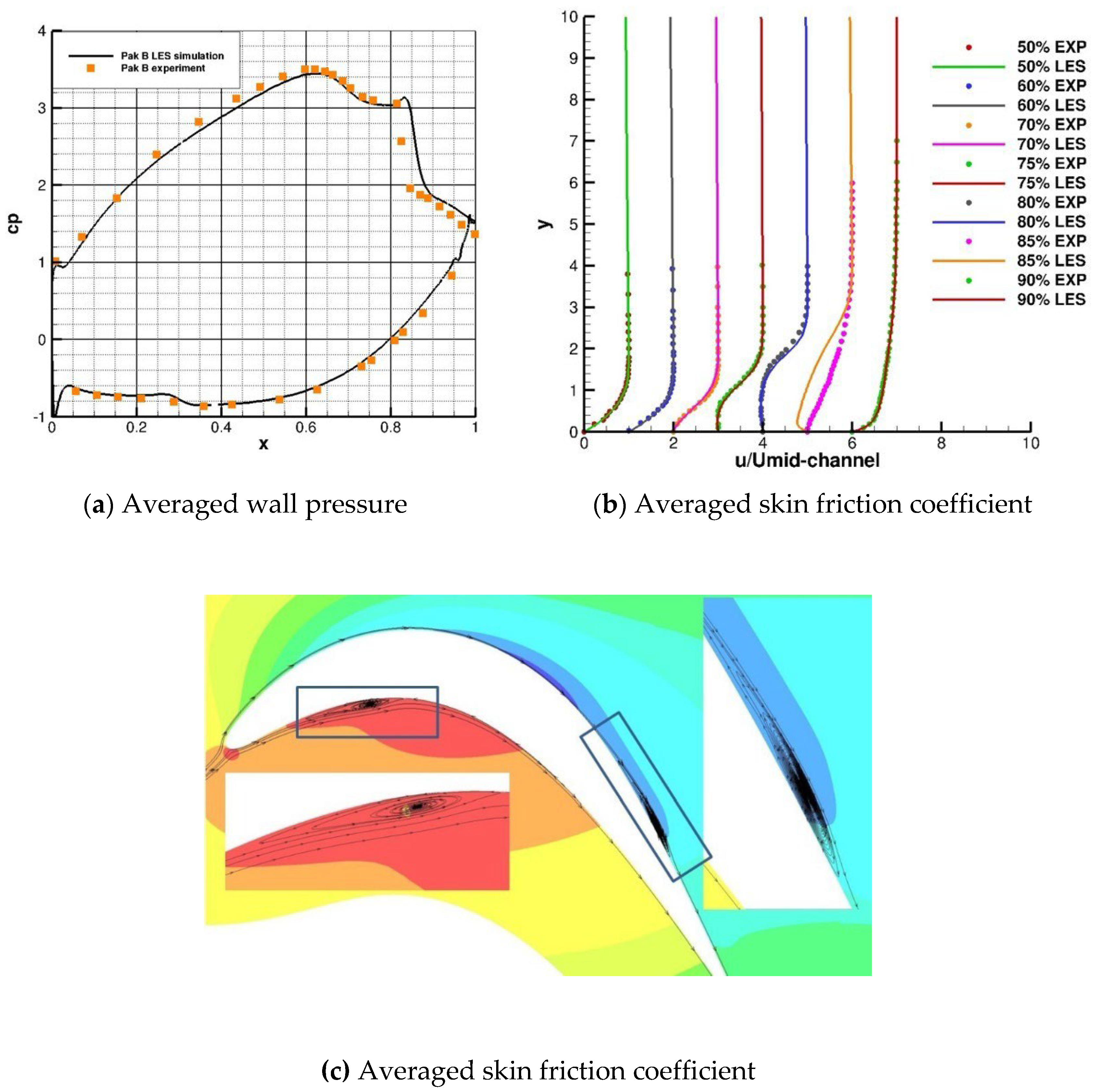
Figure 19.
The coherent structures of the suction surface.
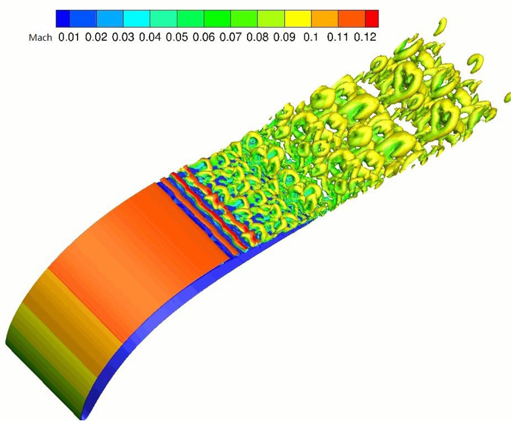

Table 1.
Main parameters of the turbulent boundary layer on the incoming plane.
| Mint | Reθ | θ/mm | δ∗/mm | δ/mm | Cf | T∞/K | |
|---|---|---|---|---|---|---|---|
| Dawson et al.[47] | 2.9 | 2400 | 0.50 | 2.85 | 6.7 | 0.00203 | 108.1 |
| Bookey et al.[48] | 2.9 | 2400 | 0.43 | 2.36 | 6.7 | 0.00225 | 108.1 |
| Wu et al.[49] | 2.9 | 2300 | 0.38 | 1.8 | 6.4 | 0.00217 | 107.1 |
| Tong et al. [50] | 2.9 | 2300 | 0.41 | 2.06 | 6.5 | 0.00256 | 108.1 |
| Present LES | 2.9 | 2400 | 0.47 | 2.37 | 6.5 | 0.00209 | 108.1 |
Table 2.
The main parameters of Pak B.
| Parameters | values |
|---|---|
| Axial chord length (mm) | 159.5 |
| Blading pitch (mm) | 141.20 |
| Flow inlet angle (degree) | 55 |
| Flow outlet angle (degree) | 30.0 |
Disclaimer/Publisher’s Note: The statements, opinions and data contained in all publications are solely those of the individual author(s) and contributor(s) and not of MDPI and/or the editor(s). MDPI and/or the editor(s) disclaim responsibility for any injury to people or property resulting from any ideas, methods, instructions or products referred to in the content. |
© 2024 by the authors. Licensee MDPI, Basel, Switzerland. This article is an open access article distributed under the terms and conditions of the Creative Commons Attribution (CC BY) license (http://creativecommons.org/licenses/by/4.0/).
Copyright: This open access article is published under a Creative Commons CC BY 4.0 license, which permit the free download, distribution, and reuse, provided that the author and preprint are cited in any reuse.


