
Submitted:
06 April 2024
Posted:
09 April 2024
You are already at the latest version
Abstract
Machine Learning deals with creating algorithms capable of learning from the provided data. These systems have a wide range of applications and can also be a valuable tool for scientific research which in recent years has been focused on finding new diagnostic techniques for particle accelerator beams. In this context SPARC_LAB is positioned, a facility located at the Frascati National Laboratories of INFN, where the progress of beam diagnostics is one of the main developments of the entire project. With this in mind, you aim to present the design of two neural networks aimed at predicting the spot size of the electron beam of the plasma-based accelerator at SPARC_LAB, which powers an undulator for the generation of x-ray Free Electron Laser (XFEL). Data-driven algorithms use two different data preprocessing techniques, namely autoencoder neural network and PCA. With both approaches, the predicted measurements can be obtained with an acceptable margin of error and most importantly without activating the accelerator, thus saving time, even compared to a simulator that can produce the same result but much more slowly. The goal is to lay the groundwork for creating a digital twin of linac and conducting virtualized diagnostics using an innovative approach.
Keywords:
beam diagnostics
; electron beam
; plasma-based accelerator
; x-ray Free Electron Laser (XFEL).
1. Introduction
The activity of the SPARC_LAB facility [1], located within the National Laboratories of Frascati of INFN, is strategically oriented towards exploring the feasibility of a high-brightness photoinjector, conducting FEL experiments [2] at ∼ 500 nm, and realizing plasma-based acceleration experiments with the aim of providing an accelerating field of several GV/m while maintaining the overall quality (in terms of energy spread and emittance) of the accelerated electron beam. Additionally, one of the fundamental developments of the entire project is the implementation of dedicated diagnostic systems to fully characterize the dynamics of high-brightness beams, which often require performing destructive measurements that interrupt machine operations. In this context, there has been a push to find a diagnostic technique that allows predicting the quality of the electron beam without activating the entire system already in the first meter of the SPARC linac accelerator. In this regard, the project introduces two neural networks that adopt the data-driven machine learning approach and implement two different data preprocessing techniques: the autoencoder network and the Principal Component Analysis (PCA). Both algorithms aim to predict the transverse spot size of the electron beam at the first diagnostic station at 1.1017 m from the gun. The proposed algorithms demonstrate their efficacy in obtaining predictions within a reasonable error range without activating the accelerator, thus saving time compared to a simulator, achieving the same results but at a much faster pace. This will enable the creation of a digital model of the entire accelerator and perform virtualized diagnostics, also in view of the EuAPS@SPARC_LAB project, which involves the realization of a structure for the use of laser-driven betatron x-ray beams [3].
2. Photoinjector and Diagnostic Measurements @SPARC_LAB
The facility SPARC_LAB, acronym for Sources for Plasma Accelerators and Radiation Compton with Laser And Beam, is a multidisciplinary laboratory with unique characteristics on the global scene located at the National Laboratories of Frascati of INFN. The research carried out focuses on experimenting with new particle acceleration techniques, such as electron plasma acceleration [4], developing new techniques for electromagnetic radiation production, such as Free Electron Laser generation [2] or THz radiation [5], and researching and implementing innovative diagnostic techniques with the aim of characterizing the obtained beam. All activities are aimed at studying the physics and applications of high-brightness photoinjectors to make future accelerators more compact and promote technological development. To understand the research work analyzed in this article, we are exclusively interested in the detailed description of the high-brightness photoinjector of the SPARC_LAB linac and the diagnostic system present in the first 1.1017 m of the accelerator.
The high-brightness SPARC photoinjector consists of a copper photocathode which, when illuminated by ultrashort pulses of high-power UV laser (266 m) with compressed energy of about 50 mJ, emits electrons via the photoelectric effect. The latter are immediately accelerated by a 1.6-cell RF gun operating in the S-band (2.856 GHz). After the RF gun, there is a solenoid with four coils, approximately 20 cm in length, necessary for focusing the electrons and opposing the space charge forces present in the non-completely relativistic beam. This element is crucial for minimizing emittance and achieving a high-brightness electron beam. Additionally, a dipole is present on the beamline for trajectory correction. Once generated and focused, the electrons are injected into three high-gradient RF accelerating sections (22 MV/m), two 3 meter long travelling wave S-band and a 1.4 meter C-band that acts as an energy booster, reaching energies of approximately 180 MeV. The line continues with experimental lines including FEL and THz generation. The layout of the entire linac is depicted in the Figure 1.
After the solenoid and dipole, specifically at 1.1017 m from the cathode, the first diagnostic station is present to monitor the characteristics of the beam produced in terms of spot size, energy and transverse emittance, obtaining extremely bright radiation pulses. The system consists of a YAG scintillating screen (AC1FLG01), transport optics and a scientific camera (AC1CAM01) with a resolution of 14 µm/pixel. The YAG Screen, an acronym for "Yttrium Aluminum Garnet," is a device that exploits the properties of crystalline materials such as aluminum garnet and yttrium to detect high-energy particles. When struck by particles, the YAG material emits a flash of light, known as "scintillation," which can be detected and recorded by light-sensitive sensors. The scintillation can be proportional to the energy of the particles, making scintillating screens useful for various experimental and diagnostic applications. In the case of SPARC_LAB, when electrons hit the scintillating flag, a flash of light is emitted which, through transport optics, intercepts the camera. By analyzing the signal, according to the camera resolution, the electron trasverse beam spot size histogram can be produced. An example of analysis is visible in Figure 2.
By analyzing the intensity of the pixels, it’s possible to measure the transverse spot size of the beam as well as the centroid and variance.It’s can also possible measure the transverse emittance using the solenoid scan thecnique. The emittance is defined as the area of the ellipse containing the particles in phase space and is closely related to the concept of brightness. Specifically, high brightness means having a high peak current (short beam), low emittance, and low energy spread (quasi-monochromatic beam). Therefore, it is important to measure it to monitor the brightness of the electron beam already at the gun. The solenoid scan technique [6,7] is described below:
- The transverse spot size of the beam on the YAG Screen for different solenoid fields is calculated as follows:where the coefficients ed are the elements of the beam line transfer matrix dependent on both the solenoid field and the YAG-solenoid distance, is the transverse spot size of the beam and it’s the divergence at the solenoid entrance. In this way, it’s possible to assess how the beam size varies with the solenoid current or field, as depicted in the Figure 3.
- The system of equations is set up, and the transfer matrix is inverted to derive , and
- The transverse emittance normalized at the entrance of the solenoid is calculated as follows:where Twiss parameters and depend on the geometry of the ellipse containing the particles in phase space.
Instead, using the centroid scan technique, the beam energy is measured. Specifically, by performing a dipole field scan and measuring the centroid of the electron beam. The trend of the measurement as a function of the dipole field is visible in Figure 4.
After interpolating the points, the slope of the line is evaluated, and the energy is measured according to the following procedure:
- The position of the dipole center is derived:
- A factor is defined:
- At the end, the energy in is evaluated:
Although relevant for determining the quality of the electron beam and extremely important for anomaly detection, both measurements described above involve beam destruction. For these reasons, scientific research is advancing alternative methods based on virtualized diagnostics. By virtualized diagnostics, you refer to a computational tool capable of providing predictions on a specific assessment, such as simulation software or a pre-trained artificial intelligence algorithm. While the time required to obtain a simulation depends on both the computational cost of the simulating machine and the mathematical computation related to the simulation itself, in the latter case, the prediction on the pre-trained network is provided almost instantaneously.
3. Neural Networks
Today, machine learning applications are increasingly widespread throughout accelerator physics. As previously mentioned, one of the innovative approaches to applying such systems to a particle accelerator is to perform virtualized diagnostics using pre-trained artificial intelligence algorithms. These tools do not use physics to produce results but provide predictions more or less accurately depending on the type of neural network used, the quality of the dataset provided and the training procedure followed [9].
Artificial Intelligence can be described as the ability of a computer system to simulate human cognitive functions using mathematical models. The science that deals with developing such models as well as creating algorithms that allow machines to learn autonomously from experience is Machine Learning, and among the computing systems primarily used in this field are Neural Networks (NN). The latter are composed of processing units called neurons connected to each other, forming a more or less complex nonlinear directed graph. The strength of the various connections is defined by a weight, a numerical value called activation defined by an activation function, evaluated through the training procedure. Knowledge is distributed precisely in the connections of the structure.
The systems just described are called "data-driven" because they heavily rely on the data provided to them. These data can be acquired from the network in raw form or pre-processed. Pre-processing can occur in various ways. Among the most well-known techniques are PCA (Principal Component Analysis) and autoencoder networks [10]. In the study intended to be described, two neural networks have been designed that use these different data pre-processing approaches to predict the transverse spot size histogram of the electron beam on the first measurement station of SPARC_LAB from the 6 machine parameters listed in Table 1.
A neural network can solve a multitude of problems. Once the goal of the designed networks is defined, it can ultimately be confirmed that what one intends to solve is a regression problem, as the aim is to interpolate the input data to associate them with features that do not represent a class. Solving a regression problem means estimating an unknown function:
through a model:
having access to some observations/data (pairs of inputs and outputs).
In the case of neural networks, where the model is parametric, it is necessary to determine the parameters, the weights, by updating them according to a training procedure. This update is performed by extrapolating information from the data and converting it into knowledge. To uncover even the smallest details, the data are iteratively analyzed, epoch after epoch, and sometimes divided into batches randomly.
To define the model, however, a loss function is used, which is usually represented by a Residual Sum of Squares (RSS):
The minimum of the loss function is the metric for searching the optimal parameter:
Finding this minimum can be costly and often it’s difficult to determine it in closed form. For these reasons, in most cases, iterative evolutionary approaches based on gradient descent are used. The gradient descent algorithm involves calculating the derivative of the loss function and subsequently updating the parameters in the direction of the decreasing gradient with a step called the learning rate. The minimum obtained with this procedure is not necessarily the absolute minimum but a local minimum that depends on the initialization. It is worth emphasizing that the choice of the learning rate is crucial: indeed, if it is too high, there is a risk of overshooting the minimum, while if it is too small, the procedure would require too many iterations. Usually, an adaptive learning rate is used, which initially is higher and tends to decrease as it approaches the minimum, avoiding situations of stagnation. Finally, to evaluate the error made by the network, it is necessary to define a metric to compare the prediction with the true data. The choice depends solely on the problem at hand. In our case, the Mean Absolute Error (MAE) has been chosen:
in order to provide a comparison between the predicted and real histograms in terms of pixel distance.
A neural network that solves a regression problem is composed by an input layer, consisting of a number of neurons equal to the size of the input data. It’s also composed by a one or more hidden layers useful for extracting salient features consisting of a variable number of neurons chosen by the designer. At the end, by an output layer that provides the prediction, consisting of a number of neurons equal to the size of the data to be predicted. The number of neurons, layers, the value of the learning rate, the choice of metric and other important parameters, defined as hyperparameters, are chosen exclusively by the designer who sets them while monitoring the loss function during training. Their choice is crucial and the convergence of the algorithm strongly depends on them as well as on the structure of the training data. In this regard, it is important to emphasize that retrieving many measurements on AC1FLG1 of SPARC in a very short time and during a continuous evolution period of the machine proved to be very difficult. Therefore, in our specific case, ASTRA simulations, one of the most well-known photoinjector simulators [8], were used for training the networks. To produce simulations consistent with the measurements made on AC1FLG1, it was necessary to initially align it with SPARC. The benchmark was performed on the emittance measurement and the result is reported in Figure 5.
The measurements converge except for a divergence beyond the waist, most likely due to machine misalignments. Using these measurements was also possible to define a conversion factor from current to field solenoid:
By performing the energy measurements in the same way, it was also possible to evaluate the conversion factor from current to dipole field:
Once the simulator was aligned with the accelerator, approximately 5000 simulations of the beam spot on AC1FLG01 were executed, simulating a beam of 10000 particles in which all 6 parameters chosen and listed in Table 1 were randomly combined. Each simulation contains the position in x and y of the simulated particles. To speed up the process, the procedure was performed through an automation script implemented in Python and executed in parallel on the Singularity facility server within the INFN laboratories in Frascati. The cluster comprises 96 CPUs and 314 GB of RAM. The scale factor from single core to cluster reduced the execution time for a simulation from 2 minutes to 2 seconds.
3.1. Preprocessing
As mentioned earlier, neural networks can be provided with data in both raw and preprocessed formats. In our specific case, it was decided to preprocess them to reduce their dimensionality and lighten the operations during training. The techniques used were PCA and the autoencoder algorithm [10]. The latter is a data preprocessing algorithm where compression and decompression functions are implemented with neural networks. Training is performed by giving the network the same examples as input and output so that it learns to encode data and then decode it in the best possible way. Being a neural network, it is closely dependent on the values of the hyperparameters chosen during construction, especially the size of the encoding. The latter represents the number of characteristic samples necessary to perform good decoding as well as the number of neurons in the last encoding layer. The mathematical principle underlying autoencoder is defined by two sets and two families of functions. The sets are the space of decoded messages X and the space of encoded messages Z, almost always Euclidean spaces. Among the functions, you find the family of encoding functions parameterized by :
and the family of decoding functions parameterized by :
For each you identify its encoding with dimension m and its decoding with dimension . An additional essential function to evaluate the performance of autoencoder is related to the quality of the reconstruction, which measures how much differs x from , called loss function. From which you obtain the optimal autoencoder using any mathematical optimization technique, usually gradient descent. For the autoencoder network used in the project, the encoding dimension m was fixed by evaluating the network’s performance in terms of loss. The chosen value is 350. A simulation is then compressed by eliminating approximately 98.25% of the redundant information. The structure of the network is fixed with an input and output layer each with 20000 neurons, one for each position in x and y of the 10000 particles from ASTRA, an intermediate encoding layer with the number of neurons equal to the chosen encoding dimension. The algorithm is trained on the Singularity facility server using ASTRA simulations, and Figure 6 shows the trend of the loss function as the epochs vary.
As can be easily observed, at each epoch, the loss decreases asymptotically approaching a minimum value closer and closer to 0, on the order of . The values of some of the hyperparameters of the network are reported in Table 2.
The PCA technique, acronym for Principal Component Analysis, is a method used to reduce the dimensionality of large data sets by employing appropriate linear combinations and transforming a large set of variables into a smaller one that still contains most of the salient information.Consider the input matrix X where each column represents one of the l data features. Also, assume that it is mean-centered (standardized) as PCA is quite sensitive to large differences between the ranges of variable definitions. At this point, a linear combination of variables is performed:
The objective is to incorporate as much information as possible into the first component, which is therefore called the first principal component. If the amount of variation in t is appreciable, then t can replace X because it can be considered a good summary of the variables. The variation in t is measured using variance, so the problem to be solved is a problem of maximizing the weights w_1, ..., w_l:
By substituting, we obtain:
Solving this linear algebra problem leads to the solution where the optimal w is the eigenvector associated with the largest eigenvalue of the covariance matrix. The second principal component is calculated in the same way provided it is uncorrelated with the first principal component, and this continues until the right trade-off between problem simplification and information loss is achieved.
Intuitively, the principal components represent geometrically the directions in which there is maximum variance, or maximum data dispersion, or maximum information. Essentially, one can think of the principal components as axes from which to better appreciate the differences between points and to discriminate which variables contribute most to the formation of the components.
It is worth noting that the principal components, precisely because they are constructed as linear combinations, have no actual meaning and are therefore difficult to interpret. Therefore, it is up to the designer to choose how many components to use based on the problem to be solved and thus the percentage of sacrificable information. In this case, a carefully chosen value of 50 was selected based on the trend shown in Figure 7.
3.2. Prediction neural networks
At this point, we can proceed with the description of the networks used to predict the high brilliance electron beam spot of SPARC. In particular, they accept 6 machine parameters as input and are trained on the measurements encoded respectively by the autoencoder network and the PCA technique to learn to predict the positions of the 10000 analyzed particles.
The implementation and development of the networks were carried out using the Python programming language version 3.7. In addition to the standard libraries already present in Python, the following packages were used:
- scikit-learn, for data standardization, PCA, autoencoder, and for the metrics used to evaluate the performance of neural networks;
- Keras, to define the sequential models of the networks, layers, and optimizers;
- matplotlib, to create plots and customize their layout.
After various algorithm tests and careful performance analysis, reasonable parameters were set for the two networks as reported in Table 3.
The number of neurons in the output layer for the network predicting the autoencoder encoding was set to 350, which is equal to the autoencoder encoding size. For the network predicting the PCA encoding, it was set to 50, which is also the number of principal components. The number of intermediate layers was chosen based on the performance of the two networks. Specifically, it was necessary to set 3 layers for the autoencoder encoding prediction network and 1 layer for the PCA encoding prediction network. Finally, the number of layers in the input layer was set to 6 for both, corresponding to the number of machine parameters from which to extract the desired prediction.
Once again, after training the algorithms on the Singularity facility server described earlier, the trends of the loss function are shown in Figure 8 and Figure 9 (insert figure number here). As can be easily observed, at each epoch, the loss decreases, tending asymptotically to a minimum value closer to 0 of the order of for both networks.
4. Results
In conclusion, the obtained results are reported and described. In particular, the predictions of the beam spot size from the two neural networks are compared with ASTRA simulations. Finally, energy and emittance measurements are performed. It is important to note that after obtaining the predictions from the two networks, it was necessary to perform a decoding to return to the original data and compare it with the simulations. For the prediction of the autoencoder network, it was sufficient to call the pre-trained decoding layer, while for pca, the compression process was reversed. While the latter must necessarily analyze all the data to be able to decompress them, the autoencoder network, after a training phase, is able to decode and encode even data it has never seen before.
Once the predictions of the positions in x and y of the 10000 particles are obtained, the comparison with the ASTRA simulations is performed on the 2D images (histograms) of the electron beam. Furthermore, to obtain a valid comparison, imagining taking the measurements directly on AC1CAM01, it was necessary to convert the size of the histogram to that of the SPARC camera frame, which is 659x494, considering the conversion factor of 0.014380 mm/pixel. The comparisons between some predicted 2D images during the test phase and the corresponding simulations are shown in Figure 10. Furthermore, analyzing the timing, it takes approximately 100 seconds to obtain a simulation from ASTRA, while it only takes around 0.5 milliseconds to obtain a prediction from the pre-trained neural network. In conclusion, the neural network makes virtual diagnostic predictions acceptably and approximately 200000 times faster than the ASTRA simulator.
For each prediction of the test set data batch, centroids and variances on x and y were calculated, and the mae trend was evaluated for both networks as a function of the training set size, visible in Figure 11 and Figure 12. This allowed us to determine the optimal cardinality. Specifically, it was set to 5000 for both networks. This result is particularly interesting because with such a small number of data points, it may be feasible to generate them directly on SPARC, making the networks a true digital twin of the first meter of accelerator.
To evaluate the performance of the two networks, measurements of emittance and energy were also performed and the results were compared with those obtained from the simulator. The machine parameters set for each of the two measurements are reported in Table 4.
In particular, a solenoid current scan was conducted over the interval 106-114 A, and the variation of spot size x was compared with the same measurement produced by the simulator. The result is visible in Figure 13. The three curves fit well near the beam waist (109 A), which is the point of interest in the search for the working point to minimize emittance. Between the predictions and the simulation, there is an error on the order of mm, a value below the resolution of the SPARC camera AC1CAM01 (14 m) and therefore not perceptible.
The measurement of energy was also carried out using the centroid displacement technique. The result is visible in Figure 14.
The slope of the line evaluated from ASTRA simulations is , it evaluated from predictions of network utilizing the PCA is and it evaluated from predictions of network utilizing the autoencoder is . The prediction of y centroid deviate from the simulation by an average error of 20.1 m for the network utilizing PCA, just over 1 pixel of error, and 2.2 m for the network utilizing the autoencoder, an error in this case imperceptible.
5. Conclusion
The aim of this work was to design two neural networks utilizing two data compression techniques, the autoencoder network and PCA, to predict the spot size of the electron beam at the first measurement station of the SPARC linear accelerator, located at the INFN National Laboratories of Frascati, starting from 6 machine parameters. Both networks were trained with simulated data from ASTRA, a photocathode simulator previously aligned with the SPARC operating point, as it was difficult to quickly obtain the desired amount of data. The idea was to lay the groundwork for creating a true digital twin of the accelerator to perform virtual measurements of emittance and energy on the photocathode.
After aligning the simulator with the accelerator, the neural networks were trained with simulated data encoded by the two analyzed techniques, the PCA and the autoencoder neural network. Subsequently, during the testing phase, both the beam spots and the emittance and energy measurements produced by the pre-trained networks and the simulator were compared.
The results obtained highlight, firstly, that both prediction algorithms require a reasonable number of simulations (5000) to be trained. This quantity could be reproduced directly on the accelerator within a few months to train on real data and create digital models of SPARC, different from the simulator especially in terms of timing to produce a prediction (∼200000 times faster) and computational cost. Furthermore, it was emphasized how the results produced by the networks using the two thecniques compared to those generated by the simulator are significant although sensitive to all machine parameters. However, an important difference between the two analyzed technique can be noted: PCA, unlike the autoencoder network, being a linear technique for dimensionality reduction, although it tries to retain the maximum variance of the original data, is unable to capture complex nonlinear relationships in the input data. For these reasons, a divergence with the simulated data was found in the energy measurement in terms of y centroid. This aspect highlights the potential of a neural network as autoencoder not only in prediction but also in preprocessing of the data.
Conflicts of Interest
The authors declare no conflicts of interest.
References
- Ferrario, M.; Alesini, D.; Anania, M.P.; Bacci, A.; Bellaveglia, M.; Bogdanov, O.; Boni, R.; Castellano, M.; Chiadroni, E.; Cianchi, A.; et al. SPARC_LAB present and future. Nucl. Instrum. Methods Phys. Res. B 2013, 309, 183–188. [Google Scholar] [CrossRef]
- Quattromini, M.; Artioli, M.; Di Palma, E.; Petralia, A.; Giannessi, L. Focusing properties of linear undulators. Phys. Rev. ST Accel. Beams 2012, 15, 080704. [Google Scholar] [CrossRef]
- Ferrario, M.; Assmann, R.W.; Avaldi, L.; Bolognesi, P.; Catalano, R.; Cianchi, A.; Cirrone, P.; Falone, A.; Ferro, T.; Gizzi, L.; et al. EuPRAXIA Advanced Photon Sources PNRR_EuAPS Project. Available online: https://www.lnf.infn.it/sis/preprint/getfilepdf.php?filename=INFN-23-12-LNF.pdf (accessed on 12 March 2024).
- Chiadroni, E.; Biagioni, A.; Alesini, D.; Anania, M.P.; Bellaveglia, M.; BIsesto, F.; Brentegani, E.; Cardelli, F.; Cianchi, A.; Costa, G.; et al. Status of Plasma-Based Experiments at the SPARC_LAB Test Facility. Proceedings of IPAC2018, Vancouver, BC, Canada, 29 April – 4 May 2018. [Google Scholar]
- Chiadroni, E.; Bacci, A.; Bellaveglia, M.; Boscolo, M.; Castellano, M.; Cultrera, L.; Di Pirro, G.; Ferrario, M.; Ficcadenti, L.; Filippetto, D.; et al. The SPARC linear accelerator based terahertz source. Appl. Phys. Lett. 2013, 102, 094101. [Google Scholar] [CrossRef]
- Scifo, J.; Alesini, D.; Anania, M.P.; Bellaveglia, M.; Bellucci, S.; Biagioni, A.; Bisesto, F.; Cardelli, F.; Chiadroni, E.; Cianchi, A.; et al. Nano-machining, surface analysis and emittance measurements of a copper photocathode at SPARC_LAB. Nucl. Instrum. Methods Phys. Res. A 2018, 909, 233–238. [Google Scholar] [CrossRef]
- Graves, W.S.; DiMauro, L.F.; Heese, R.; Johnson, E.D.; Rose, J.; Rudati, J.; Shaftan, T.; Sheehy, B.; Yu, L.-H.; Dowell, D. DUVFEL Photoinjector Dynamics: Measurement and Simulation. In Proceedings of the PAC2001, Chicago, IL, USA, 18-22 June 2001. [Google Scholar]
- Floettmann, K. ASTRA, A Space Charge Tracking Algorithm. Available online: https://www.desy.de/~mpyflo/Astra_manual/Astra-Manual_V3.2.pdf (accessed on 21 March 2024).
- Theodoridis, S. Machine Learning: A Bayesian and Optimization Perspective. In Academic Press, Inc.; Publishing House: 6277 Sea Harbor Drive Orlando, FL, United States, 2020. [Google Scholar]
- Chollet, F. Building Autoencoders in Keras. Available online: https://blog.keras.io/building-autoencoders-in-keras.html (accessed on 21 March 2024).
Figure 1.
Schematic layout of SPARC linear accelerator on SPARC_LAB facility. In detail, it’s possible to observe the structure of its first meter up to 1.1017 meters from the RF gun. In particular, there are the solenoid and dipole elements (GUNSOL, GUNDPL01) and the diagnostic system (the scintillating screen or flag AC1FLG01 and the scientific camera AC1CAM01).
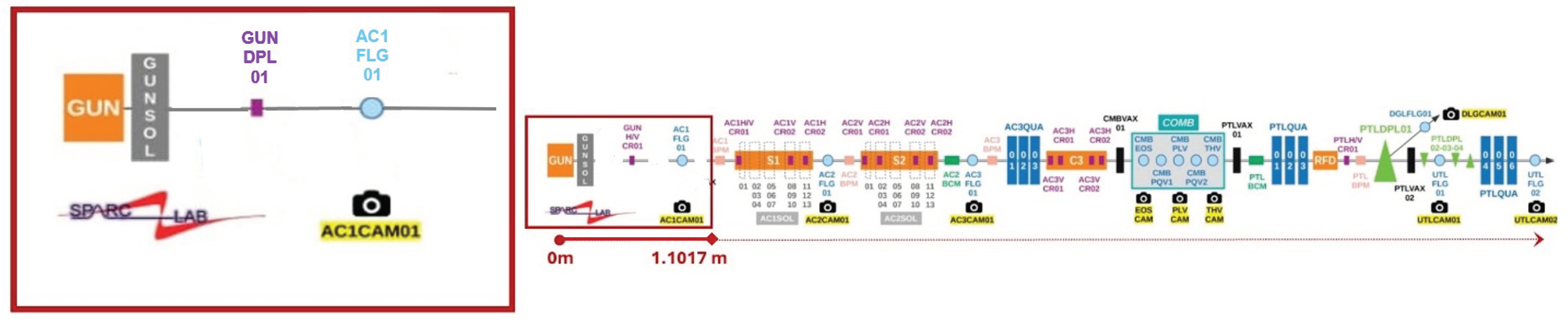
Figure 2.
In the center, the trasverse spot size of the beam, at the bottom, the particle distribution along the x-axis, and on the left, the particle distribution along the y-axis.
Figure 2.
In the center, the trasverse spot size of the beam, at the bottom, the particle distribution along the x-axis, and on the left, the particle distribution along the y-axis.
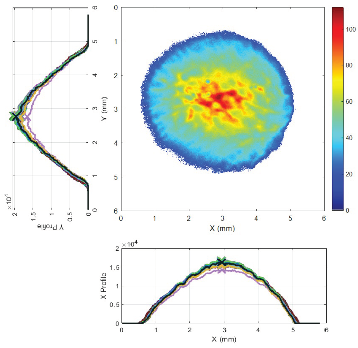
Figure 3.
Solenoid scan technique: variation of the spot size along the x-axis (RMS values) of the SPARC electron beam for a solenoid current range of 101 to 113 A.
Figure 3.
Solenoid scan technique: variation of the spot size along the x-axis (RMS values) of the SPARC electron beam for a solenoid current range of 101 to 113 A.
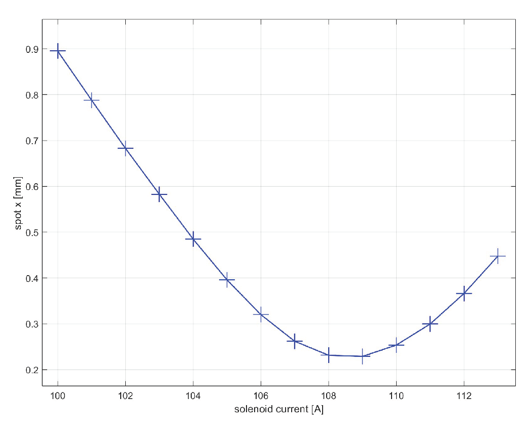
Figure 4.
Centroid scan technique: variation of the centroid along the y-axis of the SPARC electron beam for a dipole current range of -1.5 to 1 A.
Figure 4.
Centroid scan technique: variation of the centroid along the y-axis of the SPARC electron beam for a dipole current range of -1.5 to 1 A.
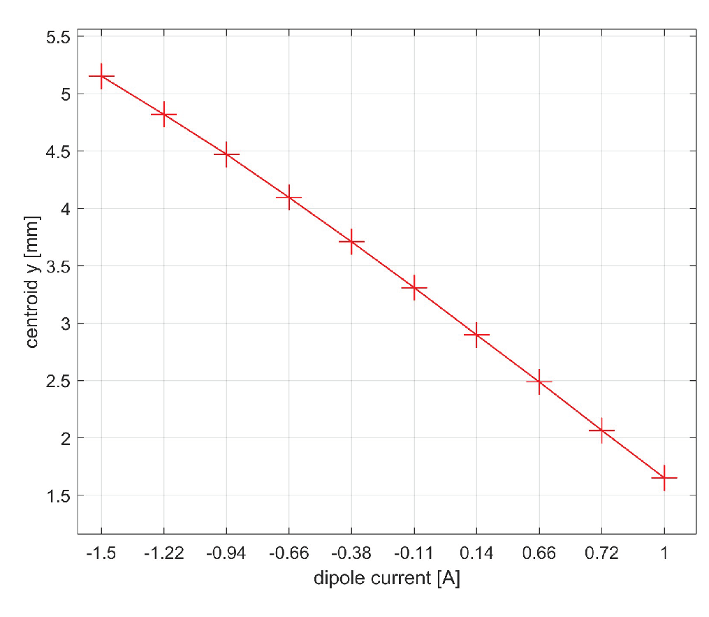
Figure 5.
Emittance measurements using ASTRA and SPARC first measure station AC1FLG01. he current scan was performed in the range 110-123 A. The measurements converge exept for the divergence beyond the waist, most likely due to machine misalignments.
Figure 5.
Emittance measurements using ASTRA and SPARC first measure station AC1FLG01. he current scan was performed in the range 110-123 A. The measurements converge exept for the divergence beyond the waist, most likely due to machine misalignments.
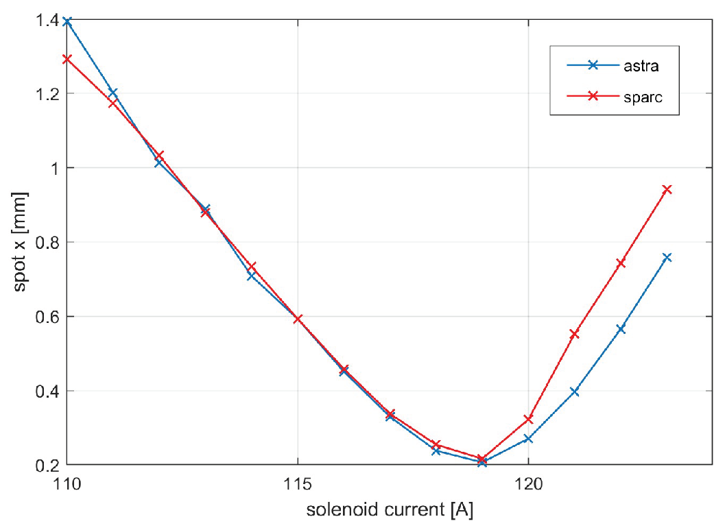
Figure 6.
Trend of the loss function of the autoencoder network as a function of epochs. The curve asymptotically approaches a value on the order of .
Figure 6.
Trend of the loss function of the autoencoder network as a function of epochs. The curve asymptotically approaches a value on the order of .
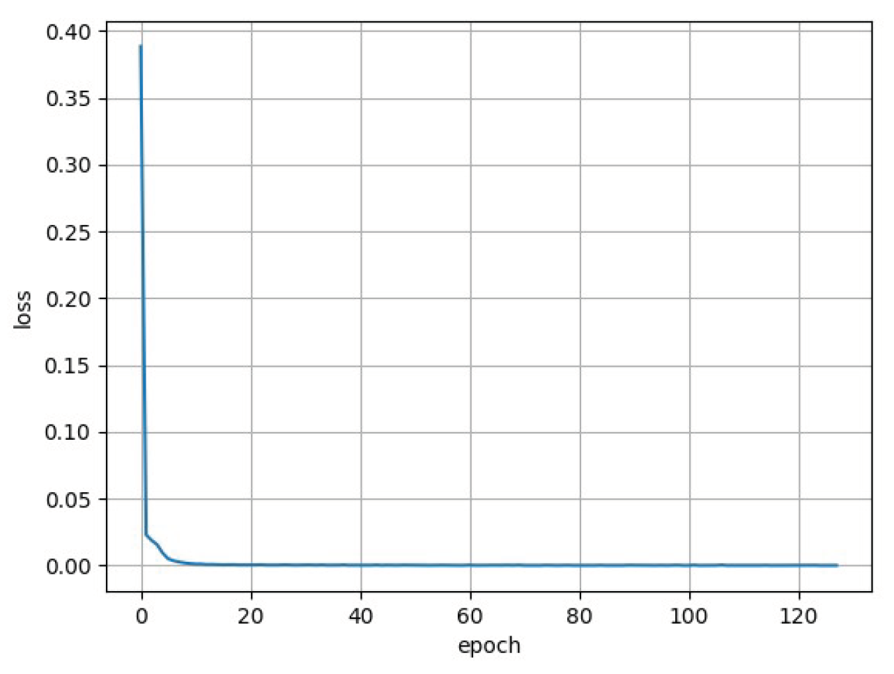
Figure 7.
Variation of the cumulative variance as a function of the number of principal components in PCA. It is inferred that the optimal number of principal components is 50.
Figure 7.
Variation of the cumulative variance as a function of the number of principal components in PCA. It is inferred that the optimal number of principal components is 50.
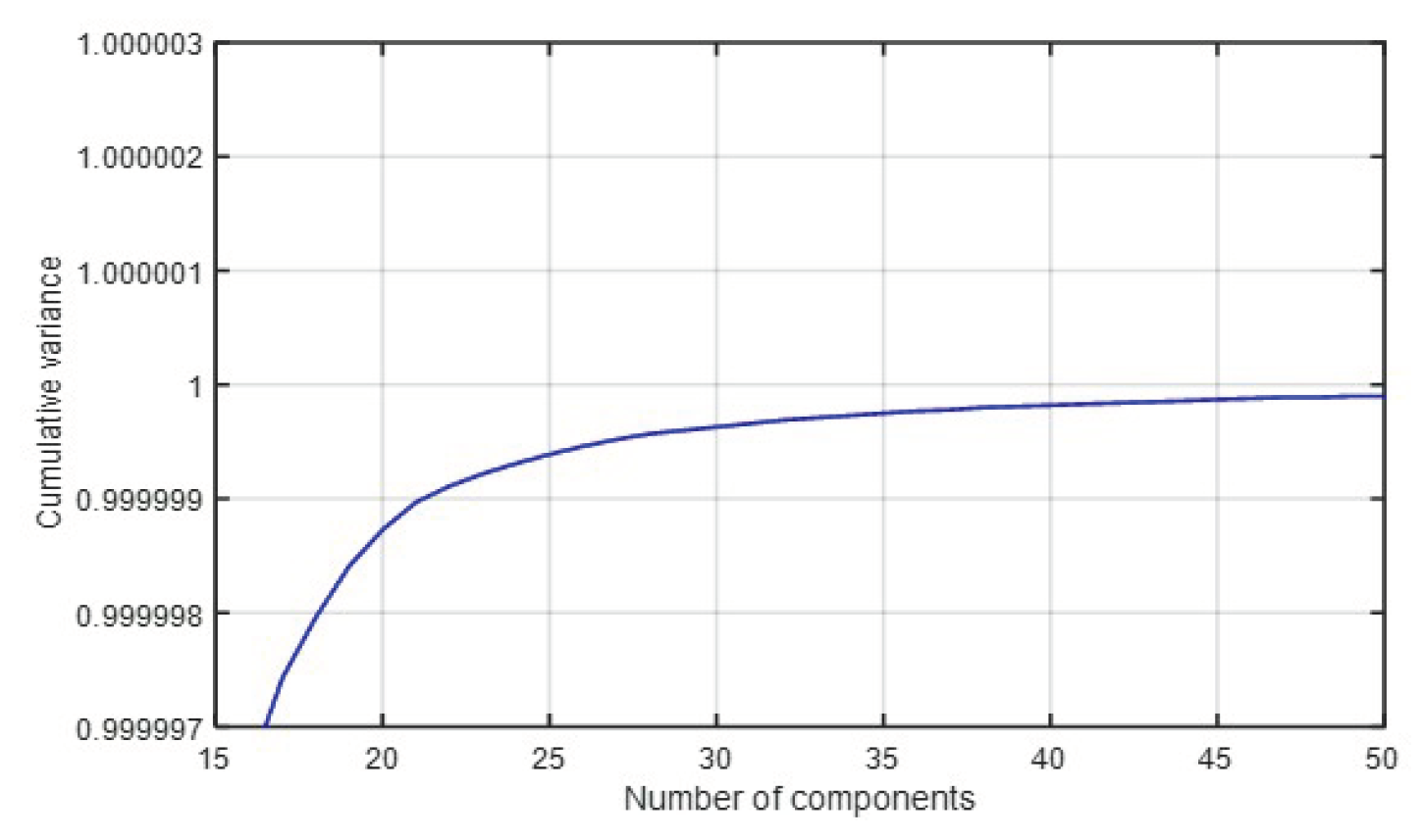
Figure 8.
Trend of the loss during the training phase as a function of the epochs of the neural network aimed at predicting the encoding of the autoencoder network.The trend asymptotically approaches the value of .
Figure 8.
Trend of the loss during the training phase as a function of the epochs of the neural network aimed at predicting the encoding of the autoencoder network.The trend asymptotically approaches the value of .
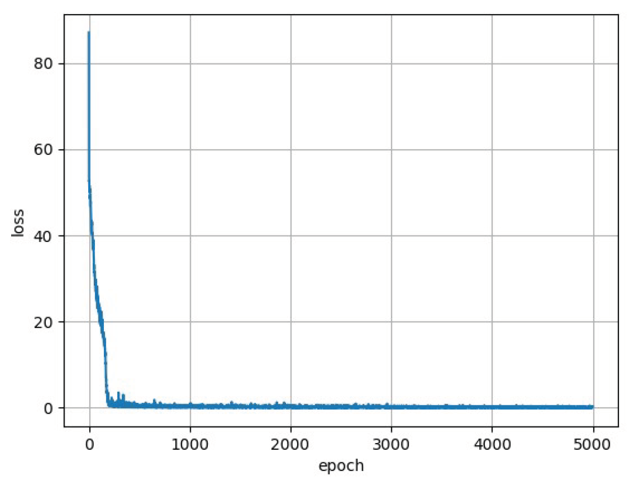
Figure 9.
Trend of the loss during the training phase as a function of the epochs of the neural network aimed at predicting the encoding of the PCA.The trend asymptotically approaches the value of .
Figure 9.
Trend of the loss during the training phase as a function of the epochs of the neural network aimed at predicting the encoding of the PCA.The trend asymptotically approaches the value of .
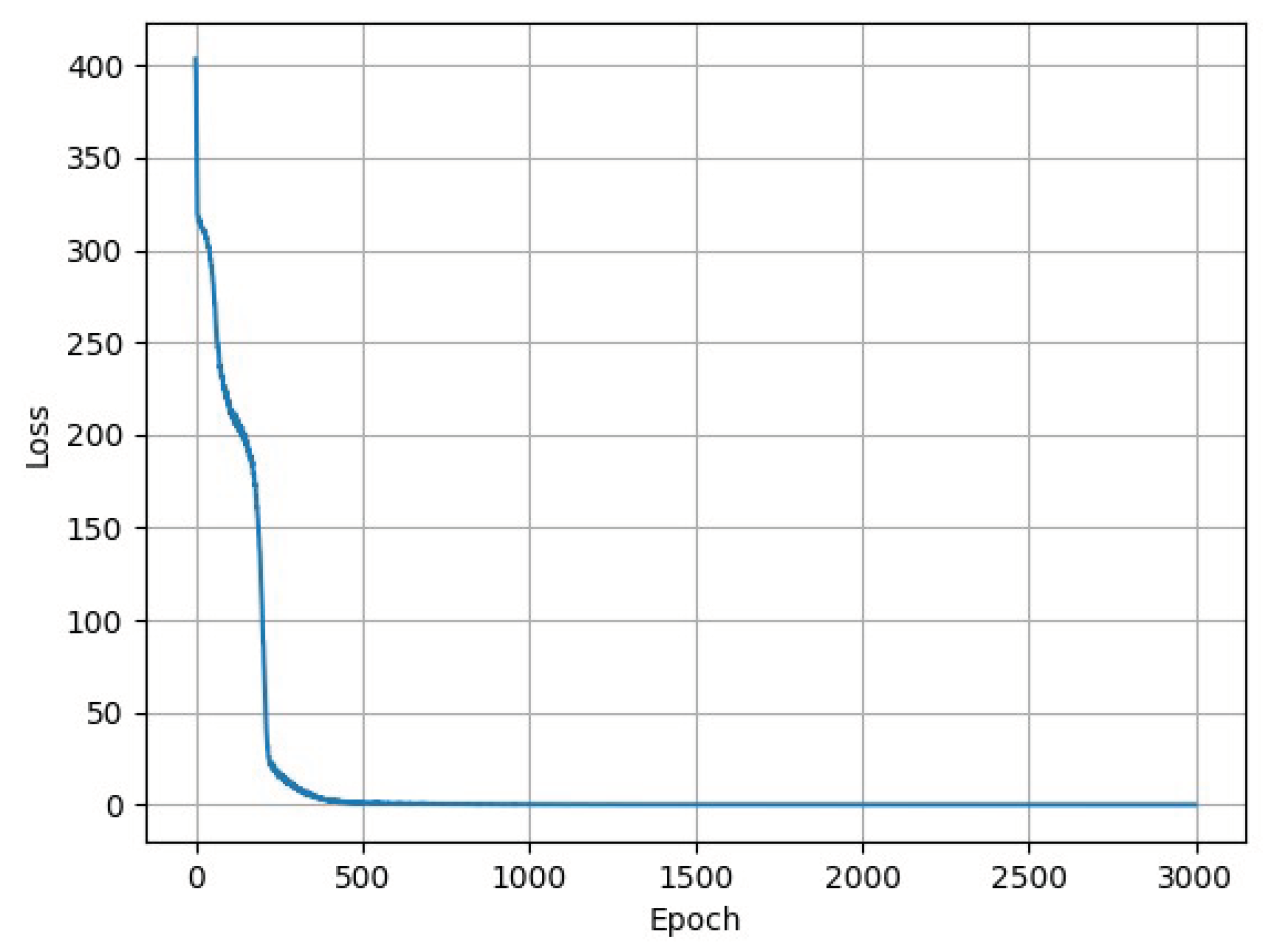
Figure 10.
Comparison of the electron beam spot size histogram simulated with ASTRA [A] and predicted with the network trained on data encoded by the PCA [B] and by autoencoder [C].
Figure 10.
Comparison of the electron beam spot size histogram simulated with ASTRA [A] and predicted with the network trained on data encoded by the PCA [B] and by autoencoder [C].
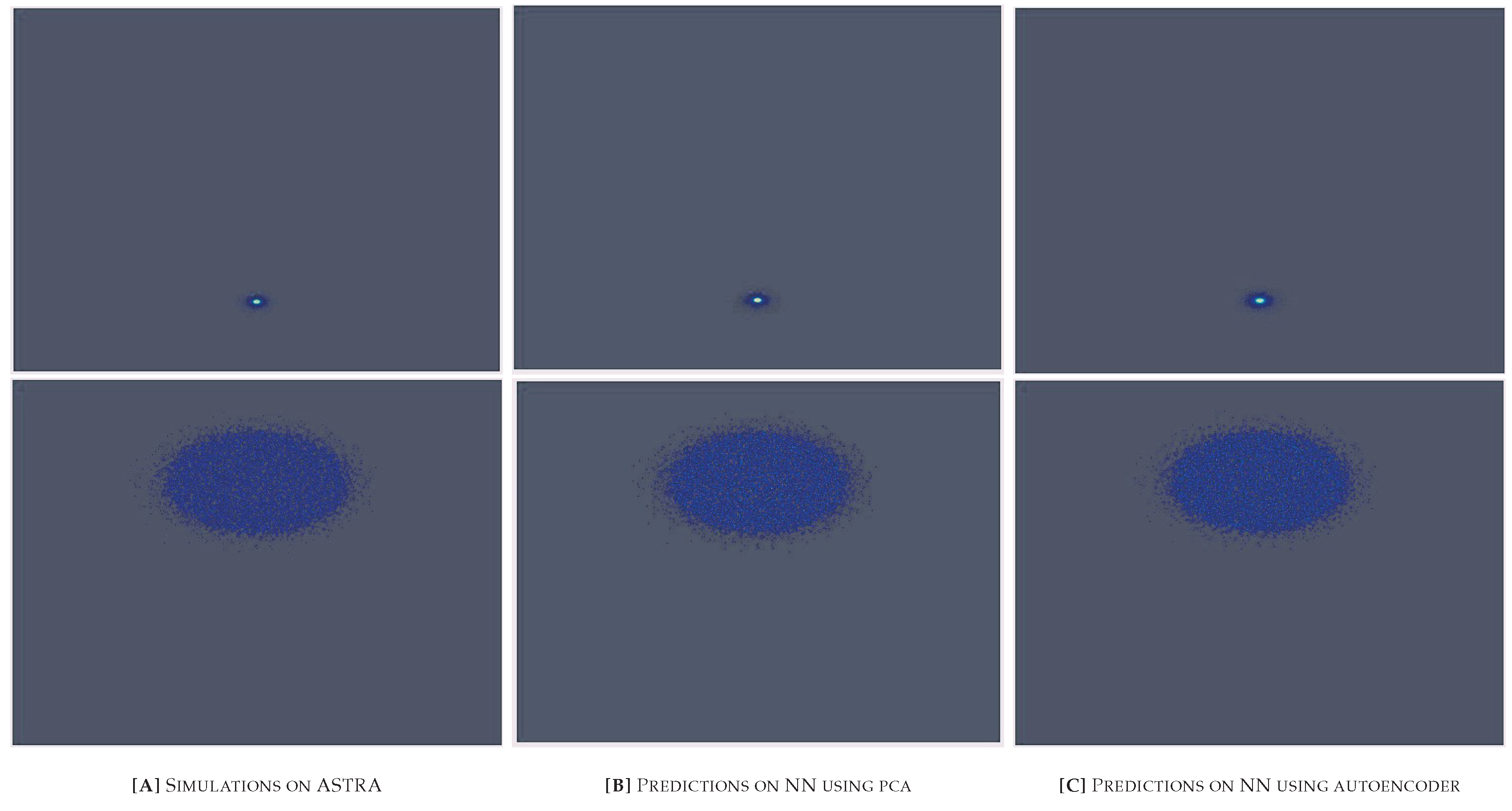
Figure 11.
Graph of the loss during training in relation to the predictions of the x and y centroids and the spot size provided by the neural network trained on the simulations encoded by the autoencoder. The red line rapresents the resolution of the AC1CAM.
Figure 11.
Graph of the loss during training in relation to the predictions of the x and y centroids and the spot size provided by the neural network trained on the simulations encoded by the autoencoder. The red line rapresents the resolution of the AC1CAM.
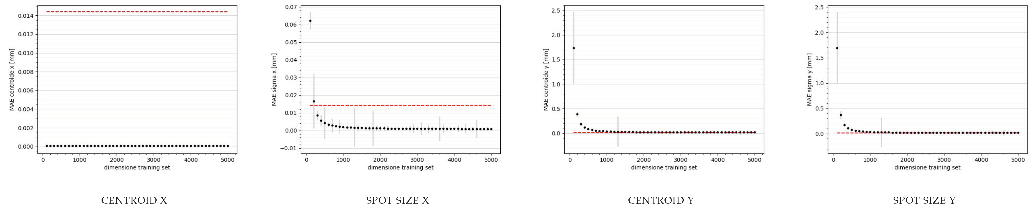
Figure 12.
Graph of the loss during training in relation to the predictions of the x and y centroids and the spot size provided by the neural network trained on the simulations encoded by the PCA. The red line rapresents the resolution of the AC1CAM.
Figure 12.
Graph of the loss during training in relation to the predictions of the x and y centroids and the spot size provided by the neural network trained on the simulations encoded by the PCA. The red line rapresents the resolution of the AC1CAM.
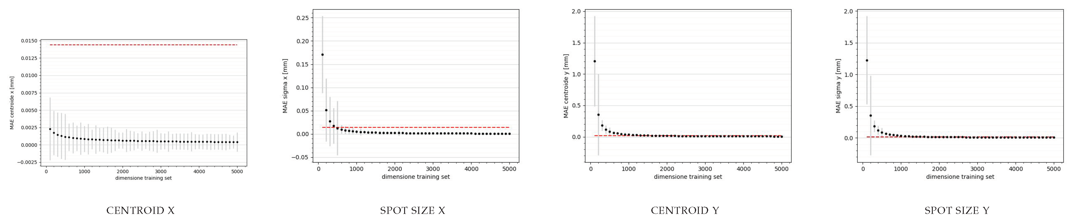
Figure 13.
Emittance measurement using solenoid scan performed on ASTRA and using both neural networks.
Figure 13.
Emittance measurement using solenoid scan performed on ASTRA and using both neural networks.
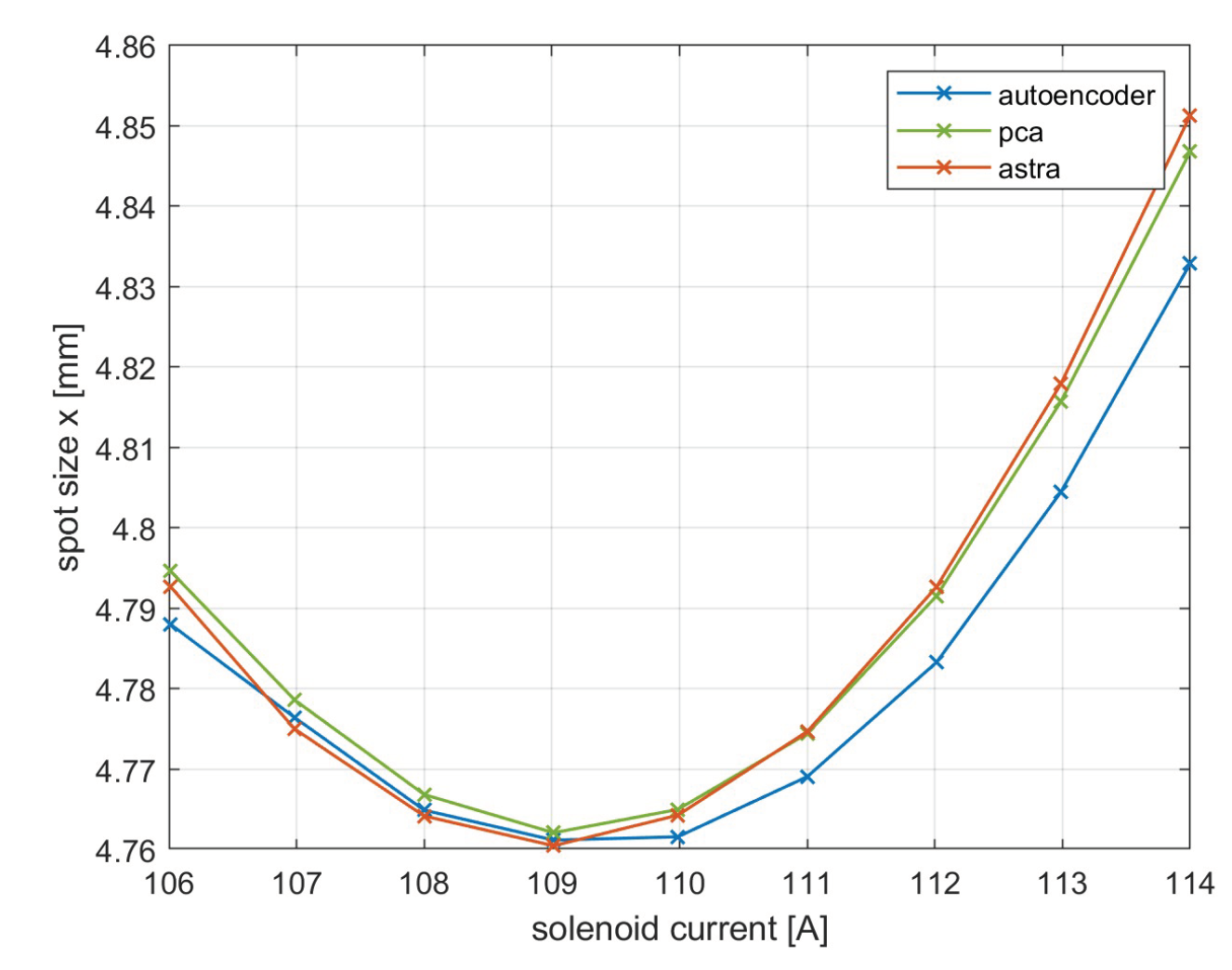
Figure 14.
Energy measurement performed on ASTRA and using both neural networks.
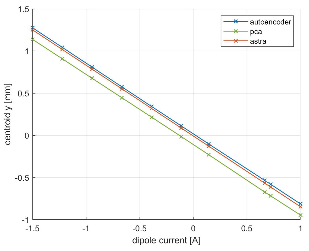

Table 1.
The 6 machine parameter and values range used to train the neural networks.
| Parameter | Variation range |
|---|---|
| laser pulse [ps] | 2.15, 2.71, 3.10, 3.68, 4.31, 4.64, 6.69, 7.94, 10 |
| laser spot [mm] | 0.21, 0.27, 0.31, 0.37, 0.43, 0.46, 0.67, 0.79, 1 |
| charge q [pC] | 10, 20, 30, 50, 80, 100, 300, 500, 1E3 |
| accelerating field [MV/m] | 115 ÷ 130 |
| solenoid field [T] | 0.28 ÷ 0.32 |
| dipole current [A] | -2.89 ÷ 2.89 |
Table 2.
Hyperparameters chosen for the autoencoder neural network. The choice was made after a careful analysis of the performance in terms of loss.
Table 2.
Hyperparameters chosen for the autoencoder neural network. The choice was made after a careful analysis of the performance in terms of loss.
| network parameters | setting |
|---|---|
| autoencoder dimension | 350 |
| learning rate (init) | 1E-5 |
| loss | mse |
| metric | mae |
| optimizer | adamax |
| epochs | 1024 |
| batch | 256 |
Table 3.
Hyperparameters chosen for the two neural networks. The choice was made after a careful analysis of the performance in terms of loss during training.
Table 3.
Hyperparameters chosen for the two neural networks. The choice was made after a careful analysis of the performance in terms of loss during training.
| network parameters | PCA | autoencoder |
|---|---|---|
| epoch | 3000 | 5000 |
| batch size | 16 | 16 |
| initial learning rate | 1E-3 | 1E-3 |
| optimizer | adamax | adamax |
| loss | mse | mse |
| metric | mae | mae |
Table 4.
Table of parameters to perform emittance and energy measurements on ASTRA and neural networks.
Table 4.
Table of parameters to perform emittance and energy measurements on ASTRA and neural networks.
| emittance | energy | |
|---|---|---|
| laser pulse [ps] | 3.69 | 7.93 |
| laser spot [mm] | 0.36 | 0.80 |
| charge [nC] | 0.05 | 0.5 |
| accelerating field [MV/m] | 120.0 | 119.0 |
| solenoid field [T] | 0.31 | 0.26÷0.28 |
| dipole current [A] | -0.5÷1 | 0.0 |
Disclaimer/Publisher’s Note: The statements, opinions and data contained in all publications are solely those of the individual author(s) and contributor(s) and not of MDPI and/or the editor(s). MDPI and/or the editor(s) disclaim responsibility for any injury to people or property resulting from any ideas, methods, instructions or products referred to in the content. |
© 2024 by the authors. Licensee MDPI, Basel, Switzerland. This article is an open access article distributed under the terms and conditions of the Creative Commons Attribution (CC BY) license (http://creativecommons.org/licenses/by/4.0/).
Copyright: This open access article is published under a Creative Commons CC BY 4.0 license, which permit the free download, distribution, and reuse, provided that the author and preprint are cited in any reuse.


