
Submitted:
07 April 2024
Posted:
08 April 2024
You are already at the latest version
Abstract
This study uses a mass-spring-damping system to simulate the repeated strain of liquefaction cyclic triaxial tests. The two results are compared in this paper to understand the feasibility of the mass-spring-damping system developed in this paper and the feasibility of future research on this related topic and development potential. The main factors affecting this mode's repeated strain are the spring coefficient k and the external force Q0. The spring coefficient has an inverse relationship but does not increase in multiples. The external force has a direct proportional relationship but does not increase the result- a non-multiple increase. When the pore water pressure of the liquefied cyclic triaxial test specimen rises, it will cause the specimen to liquefy, decreasing effective stress, shear modulus G, and damping ratio D, causing an increase in strain. The shear modulus and damping ratio are related to the spring coefficients k and c. Both are variables that change with time. This article takes an original thin-tube specimen at point A in the Yunlin area in Taiwan as a testing example. Through Mathematica software, it can be obtained that the mass m=1kg, the spring coefficient k=244e-0.1t kgf/cm, and the damping coefficient c=0.739e-0.257t kgf-s/cm and external force Q0=10.1sin2πt kg; Finally, this study selected the original thin-tube specimens from four locations in the Yunlin area, and simulated the repeated strain amount of the cyclic triaxial test specimens through a spring-damping system. The results show that the spring-damping system is feasible for simulated cyclic triaxial tests because the model is simple and the parameters are easy to understand and obtain, which also shows the extensibility of this model. Preliminary results of the research show that this model can further simulate the repeated strain obtained by cyclic triaxial tests without considering the increased trend in pore water pressure and the decrease in effective stress during cyclic loading.
Keywords:
spring-damping system
; liquefaction during cyclic triaxial test
; repeated strain
; spring coefficient
; damping coefficient
1. Introduction
Many mathematical models have been developed for analyzing ground seismic liquefaction in recent years. For the simulation target for the cyclic triaxial test, previous examples consider pore water pressure. Tropeano et al. (2019) [1] and Chiaradonna et al. (2018) [2] mentioned that simplified mathematical models can predict soil liquefaction phenomena under dynamic load. However, the correctness of the pore water pressure in the model will affect the results. Finn and Bhatia (1982), Ivšić (2006), and Park et al. (2015) [3,4,5] also mentioned three different models accompanied with damage parameters to simulate pore water pressure. The most significant difficulty in this related research is that the parameters of the mathematical model are not easy to obtain.
The mass-spring-damping system has been used in the past by Chehab and Naggar (2003) [6] to design the foundation of the hammer and press base, as well as the structural analysis between the piers and supports, both of which were based on the mass-spring-damping system. Design and analysis were commonly seen in structural dynamics-related research but less conducted in geotechnical engineering.
Kramer (1996) [7] mentioned that cyclic triaxial tests can obtain soil shear modulus (G) and damping ratio (D). Seed et al. (1986), Kaya et al. (2021), and Vargheseet al. (2019) [8,9,10] found that the damping ratio D and shear modulus G of the first five cycles will decrease as the number of cycle tests increases. These two parameters are related to the damping coefficient (c) and spring coefficient (k) in the mass-spring-damping system. Its trend can be used for more in-depth research and discussion. The parameters are easy to understand and obtain, showing the extensibility of this model, so the mass-spring-damper system could be chosen to simulate the strain of cyclic triaxial tests. Kumar et al. (2017) [11] mentioned that the damping ratio may increase with shear strain g but reverse under large shear strains. Qin et al. (2021) [12] also mentioned using a dynamic triaxial experiment to study the effect of dynamic strain on damping. The influence of the ratio: The damping ratio will decrease when the specimen increases with the dynamic strain.
Akbarimehr and Fakharian (2021) [13] studied soil materials using a cyclic triaxial instrument and mentioned that the damping ratio first decreased and then increased as the shear strain increased. Pisanò and BorisJeremić (2014) [14] also used a viscoelastic-plastic model for soil stiffness degradation and damping ratio. Chowdhury et al. (2017) [15] applied an elastic-plastic model to caisson foundations. Li and Song (2014) [16] applied it to saturated poroelastic media. Besides, Liu et al. (2021) [17] explored the nonlinear modulus and damping ratio. As for regional studies, Chattaraj and Sengupta [18] discussed Kasai River sand in India by a model.
The repeated strain of soil is generally obtained through laboratory liquefaction cyclic triaxial tests, and relevant research is conducted under the conditions of many influencing factors such as material type, particle size, gradation, etc. This paper attempted to develop a mathematical model using the mass-spring-damper system, discussed whether both the spring coefficient and damping coefficient are variables, and studies the values of various parameters of the system, including mass m, spring coefficient k, damping coefficient c, and external force Q0, and calculated using Mathematica software. Finally, the original thin-tube specimens from four locations in the Yunlin area of Taiwan were selected to conduct liquefaction cyclic triaxial tests. Then, the test results were compared with the model to investigate pattern correctness.
2. Model Developed
This study used a mass-spring-damping system to simulate the repeated strain of cyclic triaxial tests during liquefaction and investigate the related parameters of the model. Kramer (1996) [7] indicated that the formula for the mass-spring-damping system is Eq. 1.
In the formula, m is the mass, c is the damping coefficient, k is the spring coefficient, Q0 is the external force, z is the displacement, Ω is the frequency of the external force, and t is the corresponding time.
If all parameters are constants, the solution of the equation is shown in two terms. The first two terms in the equation are transitional solutions, which will tend to 0 when t >> 0, and the third is the transient solution. The formulas of the transition and transient solutions can also be found in Kramer's book (1996) [7]. The total solution is shown in Eq. 2, which is the sum of the transition and steady-state solutions. The transition solution can be obtained by Eq. 3, which is an unstable solution that changes irregularly with time. The steady-state solution can be obtained by Eq. 4, A stable solution that trends as a sinusoidal function over time.
where, natural frequency , damping ratio , damping ratio natural frequency ,
3. Parameter Study
To verify the correctness of the model, the samplers were selected, and boring sites were found in the Tuku and Huwei areas in Yunlin, Taiwan. In 1999, the 921 Chi-Chi earthquake massacred the central regions of Taiwan. The earthquake epicenter was about 20 km away from this sampling site base. Dozens of people were killed in the Yunlin area at that time. Hwang et al. (2003) and Chang et al. (2011) [19,20] conducted a liquefaction analysis in the Yunlin area of the 921 Chi-Chi earthquake. In recent years, Fansuri et al. (2022) and Chiou et al. (2021) [21,22] also conducted follow-up related research on the Yunlin area. Figure 1 shows the sampling base site and the location of the Yunlin area in Taiwan. This study selected four locations for drilling and sampling. Subsequently, the original thin-tube specimen at site A will be used as the result of the reference example. In this study, undisturbed thin-tube specimens from four locations in Yunlin, Taiwan, were selected to simulate the strain of the specimen through a mass-spring-damping system, namely sites A, B, C, and D. Their locations are shown in Figure 1; the test specimens were selected based on the liquefaction potential value (LPI) obtained through the relevant physical properties and SPT N value test results. This study selected two test specimens in the medium liquefaction potential area and two in the high liquefaction potential area. Table 1 shows cyclic triaxial test results of twelve specimens taken from four sites. Four specimens will be further analyzed for the strain value by the mass-spring-damping system to compare those of cyclic triaxial test specimens. Das (1993) [23] explained boring and sampling very clearly. Kaya and Erken (2015) and Bray et al. (2017) [24,25] also used the thin-tube method to obtain the samplers to be tested afterward. We also referred to their suggestion and requirements during the boring and sampling period.
3.1. Parameters Are Constant
When all coefficients are constants, the solution of the problem is as Eq. 2. The first two terms in Eq. 3 are transitional solutions and will tend to 0 when t >> 0; the first two terms can be regarded as 0, so only the third term in Eq. 4 can be calculated to obtain the displacement. Meantime, Eq. 4 can be found that the spring coefficient (k) and the damping coefficient (c) are located in the denominator and are inversely proportional to the displacement. It means that if the maximum value of the constant is substituted, then the displacement obtained will be the minimum. However, it can be known from the concepts of rising pore water pressure and falling effective stress that both variables of the spring coefficient k and the damping coefficient c will change with time. Once the spring and damping coefficients are substituted as variables, it cannot be directly solved through Eq. 2. However, it can be inferred from the above. When the spring coefficient (k) and damping coefficient (c) decrease as time increases, the displacement will increase accordingly. Besides, as the analytical solution cannot be obtained directly, we will use Mathematica software to find the numerical solution for the differential equation.
3.2. Parameters k and c Are Variables Depending on Time
The parameters required for the mass-spring-damping system to simulate the strain of cyclic liquefaction triaxial tests are mass, spring coefficient, damping coefficient, and external force, which can be determined by the increase in pore water pressure and the decrease in effective stress. The concept can be used to obtain parameters corresponding to different specimens; when the pore water pressure of the specimen in cyclic triaxial tests increases, it will cause the specimen to liquefy, causing the effective stress, shear modulus G, and damping ratio D to decrease, causing the strain to increases, and the shear modulus G and damping ratio D are related to the spring coefficient k and damping coefficient c respectively. Both are variables that change with time. This study uses the original thin-tube specimen at site A in the Yunlin area as an example for parameter calculation. Akbarimehr and Fakharian (2021) [13] mentioned the relationship between stiffness degradation, damping, and shear strain. Pisanò and Jeremić (2014) [14] also mentioned the relationship between stiffness degradation and damping.
3.2.1. Mass
The mass of point A is calculated as follows. The mass (m) is calculated by multiplying the volume of the specimen in the cyclic triaxial test by the unit weight of the soil. It is known that the diameter and height of the specimen are 7.1cm and 14.2 cm, respectively. Thus, the calculated volume is 562.2 cm2. The unit weight of the cyclic triaxial test specimen could change with the soil gradation or soil types, generally in the range between 1.9 and 2.12 g/cm3 in Table 1. After multiplying the volume of the specimen by the unit weight, the available mass heavier than most soils generally falls between 800 and 1000g, so each specimen's mass m is defined to be 1kg in the study.
3.2.2. Spring Coefficient
The spring coefficient (k) of the reference sampler A is calculated by dividing the force F by the length change ΔL, as shown in Eq. 5, where the force and the length change are computed at a strain of 1%. When calculating the external force, the axial differential stress ) in the formula is obtained from the static triaxial undrained CU test results of Hsiao et al. (2015) [26]. It is found that the axial differential stress 78 kPa can be obtained at the 1% strain.
In the formula, the force F = ) × A, the axial difference stress is calculated at a strain of 1%. The obtained axial differential stress ) is 78kPa, and we can convert it to 0.78 kgf/cm2. Based on specimen area equaling 39.59 cm2, we can find F=30.88kg. Meantime ΔL=ε×L=0.01×14.2cm=0.14 cm. The spring coefficient k can be obtained by dividing the force F obtained above by the length change ΔL. Using Eq. 5, the spring coefficient (k) is calculated as 220 kgf/cm, the spring coefficient of the first cycle. Many papers [27,28,29] mentioned that G or E value decreases with increasing strain. However, few papers mentioned the relationship between k and strain. The model in this article requires the relationship between k value and strain; the strain increases due to the variation of k value as the cyclic number increases. We used the relationship between G and the cyclic number as the relationship between spring coefficient k and the cyclic number.
After the first cycle's spring coefficient is calculated, the shear modulus (G) of the first five cycles of the specimen at A-2 is calculated, as shown in Table 2. The shear modulus (G) curve equation, which is G=5884.9e-0.1t kPa, is solved in Table 2 with the help of a command in Excel.
This study uses the shear modulus (G) curve equation of the first five cycles at point A as the basis for the spring coefficient (k) curve equation. The spring coefficient (k) of the first cycle is brought in from the above calculation k=220 kgf/cm; a spring coefficient (k) curve equation similar to the shear modulus (G) curve equation can be obtained, as shown in Figure 2. Since the number of liquefaction times of the sample at point A is 15, the number of cycles on the horizontal axis is changed to 15. Point A's spring coefficient can be obtained from this method as k=244e-0.1t kgf/cm. The spring coefficient is a variable that changes with time and will decrease as time increases. Table 2 uses the above spring coefficient equation to calculate the values for each of the 15 cycles.
3.2.3. Damping Coefficient
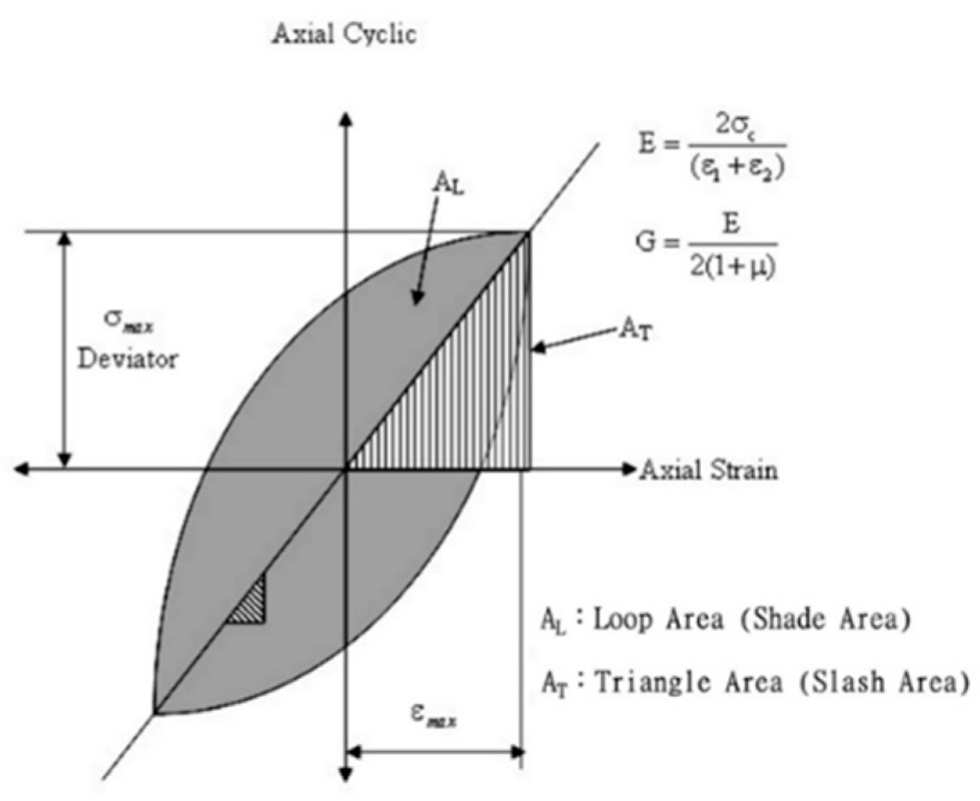
Kumar et al. (2017) and Akbarimehr and Fakharian (2021) [11,13] both mentioned the damping ratio (D) analysis method, such as Eq. 6.
In which AL is the area of the hysteresis loop, and AT is the area of a shaded right triangle. AL can be calculated by ()、()、().... () into Eq. 7
Figure 3.
Stress-strain loop under load amplitude.
The damping coefficient c of site A is calculated in Figure 4. The damping ratio D obtained for each cycle of the cyclic triaxial test results of the specimen at site A is written in Table 3. Use the Excel trend line command to draw a set of equations directly used as the basis for the damping coefficient (c). Since the number of liquefaction times of the sample at point A is 15, the number of cycles on the horizontal axis is changed to 15, as shown in Figure 4. Point A's damping coefficient (c) can be obtained from the method as c=0.739e-0.257t kgf-s/cm. Table 3 uses the above damping coefficient equation to calculate the damping coefficients for 15 cycles.
The external force (Q0) calculation formula at point A is extended from Eq. 8. The first cyclic spring coefficient (k) of point A can be obtained from k=220kgf/cm stated before, multiplied by the strain of the first cycle of the specimen (ε=0.323%), height (L=14.2cm), and sin2πt, as shown in Eq. 8, the strain of the first cycle of the specimen is, and the external force in the liquefaction repeated triaxial test is a sinusoidal function cyclic loading. This study added sin2πt to the external force equation to simulate the cyclic triaxial test. Hence, Q0 is 10.1sin2πt kg.
3.3. Numerical Method to Solve it
After calculation by the above method and substituting each parameter into Equation 1, the formula of the sample from site A in the mass-spring-damping system can be obtained as Eq. 9. Then, the specimen's strain will be solved by calculating it with Mathematica software.
First, enter the NDslove in the Mathematica command. The NDslove command is used to solve the numerical solution of a differential equation with variable coefficients. The result is a graph. The equation to be calculated, boundary conditions, and the range of variables need to be entered in the command. The equation to be calculated takes A-2 as an example, such as Eq. 9. The boundary conditions in this study are set to 0 and 2. As for the range of time variable, because the cyclic number of liquefaction of the sample at point A approaches 15, we set the time to 15. After the graph of the NDslove results is solved, use the Plot command to draw the graph. In the Plot command, you also need to enter the range of the variables and the parameters to draw the graph. Since the number of liquefaction times of the sample at point A is 15, the range of the variables is The time (t) is set to 15. After the above two steps, the numerical solution of the quadratic differential equation with variable coefficients required in this study can be obtained.
To verify that the numerical solution obtained by the calculation software Mathematica is consistent with the analytical solution calculated using mathematical formulas, this study first sets up a simple quadratic variable coefficient differential equation, such as Eq. 10, by using Laplace transform and the calculation software Mathematica 12.1 to solve the problem, and by comparing the results, we can know the feasibility of Mathematica being used in the calculation of this study.
Substituting 0.2 for c in the Eq. 10, after calculating the analytical solution through Laplace transformation, use Excel to draw it and compare it with the numerical solution in Mathematica. Both times (t) are t=5sec. Substitute into the calculation, Figure 5 is a comparison chart of the Laplace transform and Mathematica results. It can be found that the two curves are consistent, so it can be verified that Mathematica is the calculation software that can be applied to this research.
3.4. Parameter Study
This part mainly discusses the parameters of the mass-spring-damping system, mass (m), spring coefficient (k), damping coefficient (c), and external force (Q0). The parameters used are based on point A in section 3.2. This is the result of the baseline calculation, which is reduced ten times and enlarged ten times one by one to discuss the impact on the simulated displacement of the mass-spring-damping system. The parameters discussed are as follows in Table 4.
3.4.1. Effect of Mass on Repeated Strain
In the beginning, the impact of changing the mass size (m) on the displacement of the mass-spring-damper system simulation is discussed. For this type, the mass (m) uses the calculation result m=1kg in Section 3.2.1 as the original data. It reduces it by ten times and enlarged ten times, two different sizes of mass (m) can be obtained, m=0.1kg and m=10kg, respectively F1 to F3, as shown in Table 5, to explore the influence on simulated strain for the mass-spring-damping system.
Bring the three sets of parameters obtained above into the mass-spring-damping system for calculation and explore the impact of reducing the mass (m) by ten times and enlarging it by ten times on the strain. After calculation with Mathematica software, the displacements from F1 to F3 can be obtained. The volume versus time graph is shown in Figure 6.
It can be seen from Figure 6 above that based on the F1 original data m=1kg, when the mass (m) is reduced ten times, the strain will be enlarged, and when the mass (m) is enlarged ten times, the displacement will be slightly reduced. Such a result can be imagined. When the size of the sample container is fixed, the relative density will increase as the mass increases. Thus, the strength will also increase, and the strain will decrease. This analysis results can be verified.
3.4.2. Effect of Spring Coefficient on Repeated Strain
Next, we will discuss the impact of changing the spring coefficient (k) on the simulated displacement of the mass-spring-damping system. For this type, the spring coefficient (k) is calculated based on the result k=244e-0.1t kgf/cm in Section 3.2.2. Original data, reduced ten times and enlarged ten times, two different sizes of spring coefficients (k) can be obtained, k=24.4e-0.1t kgf/cm and k=2440e-0.1t kgf/cm, respectively G1 to G3, as shown in Table 6, to explore the impact on the simulated strain of the mass-spring-damping system.
Next, we will discuss the impact of changing the spring coefficient (k) on the simulated displacement of the mass-spring-damping system. For this type, the spring coefficient (k) is calculated based on the result k=244e-0.1t kgf/cm in Section 3.2.2. Original data, reduced ten times and enlarged ten times, two different sizes of spring coefficients (k) can be obtained, k=24.4e-0.1t kgf/cm and k=2440e-0.1t kgf/cm, respectively G1 to G3, as shown in Table 6, to explore the impact on the simulated strain of the mass-spring-damping system.
It can be seen from Figure 7 above that based on the original data of G1 k=244e-0.1t kg/cm; the displacement will be affected by the increase or decrease of the spring coefficient (k), which is an inverse but non-multiply relationship.
3.4.3. Effect of Damping Coefficient on Repeated Strain
We continued to discuss the impact of changing the damping coefficient (c) on the simulated displacement of the mass-spring-damping system. For this type, the damping coefficient (c) is calculated in Section 3.2.3, and the result is c=0.739e-0.257t kgf-s/cm is the original data, which is reduced by ten times and enlarged by ten times, respectively. Two damping coefficients (c) of different sizes can be obtained, c=0.0739e-0.257t of-s/cm and c=7.39e-0.257t kgf-s/cm, respectively H1 to H3, as shown in Table 7, to investigate the influence on the simulated strain of the mass-spring-damping system.
The above three sets of parameters were inserted into the mass-spring-damping system for calculation, and the impact of reducing and enlarging the damping coefficient c by ten times on the displacement was explored. After calculation with Mathematica software, the displacements from H1 to H3 can be obtained. The time graph is shown in Figure 8.
It can be seen from Figure 8 above that based on the H1 original data c=0.739e-0.257t kgf-s/cm, it can be found that the impact of the damping coefficient on the displacement could not be more precise.
3.4.4. Effect of External Force on Repeated Strain
Finally, the impact of changing the size of the external force (Q0) on the simulated displacement of the mass-spring-damping system is discussed. For this type, the external force is reduced using the calculation result Q0=10.1 sin2πt kg in section 3.2.4 as the original data. Ten times and ten times magnification, two different sizes of external forces Q0 can be obtained, Q0=1.01sin2πt kg and Q0=101sin2πt kg, respectively I1 to I3, as shown in Table 8, to discuss the mass-spring-damping system when simulating the effect of the strain.
Substitute the above three sets of parameters into calculating the mass-spring-damping system to explore the impact of reducing the external force (Q0) by ten times and amplifying it by ten times on the displacement. After calculation with Mathematica software, the displacements from I1 to I3 and The time chart are shown in Figure 9.
From Figure 9 stated above, we know that based on the original data of I1 Q0 = 10.1 sin2πt kg, the strain will be affected by the increase or decrease of the external force (Q0), and the two are proportional and seem not multiples.
From the preceding content, the summary of parameter analysis can be summarized as follows:
- Mass (m) is a constant. According to the comparison result of changing the size of mass m, it can be found that it is inversely proportional to the displacement and is not a multiple. When the mass is reduced ten times, the displacement will be enlarged, and when the mass is reduced by ten times, the displacement will be enlarged. When the mass is enlarged ten times, the displacement will be slightly reduced.
- The spring coefficient (k) is a variable that changes with time. According to the comparison results of changing the spring coefficient k, it can be found that the displacement will be affected by the increase or decrease of the spring coefficient in an inverse proportion and not a multiple relation.
- The damping coefficient (c) is a variable that changes with time. According to the comparison results of changing the damping coefficient c, the impact of the damping coefficient on displacement could be more apparent.
- The external force (Q0) is the cyclic load multiplied by Sin2πt. According to the comparison results of changing the magnitude of the external force Q0, it can be found that the displacement will be affected by the increase or decrease of the external force in a proportional and non-multiple relationship.
- After reducing and enlarging the original data of spring coefficient k and damping coefficient c ten times and discussing, respectively, the influence of each parameter on the displacement can be obtained, as shown in Table 9.
4. Results and Discussions
Xu et al. (2021) [30] once analyzed and compared the model and test results of undrained repeated triaxial tests on densely saturated sand with different particle sizes and fine content. They also used the equivalent granular state parameter to discuss the model parameters.
4.1. A Site
Point A is located in Huwei Town, Yunlin County, with a sampling depth of 5.0-5.75m and a groundwater level of 2.3m. The soil sample A-2 belongs to a poorly graded sandy soil, and it is classified as SP according to the USCS method. The soil unit weight is 2.02t/m3, the water content is 16.09%, and the specific gravity is 2.76. Figure 10(a) shows the soils liquefied at 15 cyclic times. Figure 10 (b) indicates soil grain size distribution, from which most local soils are sandy soils, but the curve shows most soil particles almost contain a little fine. The shrinkage of the sample during cyclic loadings is not apparent for the A-2 specimen in Figure 10(c), and we can find that the initial liquefaction occurred in the 10th cyclic number from the excess pore water developed curve in Figure 10(d). Figure 10(e) displays the double strain of the specimen with respective cyclic axial strain. Figure 10(f) is the stress-strain diagram of the first five cycles for A-2. Only the first five cycles are used because they are easier to analyze, and the analysis results are more accurate. The shear modulus of the first five cycles can be obtained, and click on each to get the shear modulus curve. The spring coefficient k of A-2 can be obtained as k=244e-0.1t kgf/cm. Due to liquefaction, the cyclic number of times is 15. The damping coefficient (c) of A-2 directly uses the damping ratio curve trend as the basis for the damping coefficient, and the damping ratio curve is obtained from the previous five cycles in Figure 10(f). The damping coefficient c of A-2 can be c=0.739e-0.257t kgf-s/cm, since the number of liquefaction times is 11.
The mass m, damping coefficient c, spring coefficient k, and external force Q0 of point A are brought into the mass-spring-damping system calculation and compared with the liquefaction repeated triaxial test results, as shown in Figure 11. The strain of the first four cycles simulated by the mass-spring-damping system at point A has a relatively irregular amplitude, and the strain peak will have an upward trend as the number of cycles increases. The strain was obtained through repeated liquefaction triaxial tests. The peak value is flat, with no upward trend. After the eleventh cycle, there will be a more noticeable difference between the two. This may be related to the cumbersome simulation process and soil properties such as acceptable material content and ratio. The stress-strain diagram of this specimen is similar to taking the upper end of the block circle as the vertex and rotating clockwise from the lower left to the upper left; it is different from the stress-strain diagrams of the other three specimens.
4.2. B Site
Point B is located in Tuku Town, Yunlin County, with a sampling depth of 5.0-5.75m and a groundwater level of 2.3m. The soil sample B-2 is fine-graded silt-containing sand, SW-SM. The soil unit weight is 2.02t/m3, the moisture content is 22.44%, and the soil specific gravity is 2.69. we can obtain the cyclic number 18 when initial liquefaction in Figure 12(a). Figure 12 (b) shows soil grain size distribution, from which most local soils are sandy soils, but the data show all the soil particles passing 1 mm. The shrinkage is apparent and quick for the B-2 specimen in Figure 12(c), although the initial liquefaction seems not to have occurred from the excess pore water developed curve in Figure 12(d). Figure 12(e) displays the double strain of the specimen with respective cyclic axial strain. The results are similar to those of Figure 10(e). Figure 12(f) shows the stress-strain diagram of the first five cycles at point B. Only the first five cycles are used because they are easier to analyze, and the analysis results are more accurate. The result is the first cycle's spring coefficient k. The trend of the shear modulus G curve is the basis for the first cycle spring coefficient. The spring coefficient k of B-2 can be obtained as k=269e-0.2t kgf/cm because liquefaction times are 18 times. The damping ratio curve is obtained from the previous five cycles. The damping coefficient c of B-2 can be obtained as c=0.298e-0.114t kgf-s/cm.
The mass m, damping coefficient c, spring coefficient k, and external force Q0 of point B are brought into the mass-spring-damping system calculation and compared with the results of the liquefaction repeated triaxial test, as shown in Figure 13. The strain peak value simulated by the mass-spring-damping system at point B increases as the number of cycles increases, but the strain peak value decreases at the eighth cycle. The strain peak value obtained through cyclic liquefaction triaxial tests rises more smoothly, and no shrinkage trend exists. There is a significant difference between the two in the first eight cycles. This may be related to the stress reduction and pore water pressure trend. The stress of the specimen reaches the fifth cycle. After that, it decreased significantly, and the pore water pressure only rose to 45kPa, which did not get the failure point of 90kPa.
4.3. C Site
Point C is located in Huwei Town, Yunlin County, with a sampling depth of 5.0 to 5.8m and a groundwater level of 3.6m. The soil sample C-1 is poorly graded sand, SP-SM. The soil unit weight is 2.12t/m3, and the moisture content is 23.33%; soil specific gravity is 2.69. The sample C-1 was applied with an effective confined pressure of 100 kPa, and the cyclic stress ratio (CSR) is 0.265; then, we can obtain the cyclic number 9 when initial liquefaction in Figure 14(a). Figure 14 (b) shows soil grain size distribution, from which most local soils are sandy soils, but the fines content is very low. The shrinkage is apparent and quick for the C-1 specimen in Figure 14(c), although the liquefaction cyclic number is seven from excess pore water data in Figure 14(d). However, Figure 14(e) displays that the double strain is from 2% to -2% during cyclic loadings and does not have considerable axial strain. Figure 14(f) below is the stress-strain diagram of point C for each cycle. Only the first five cycles are used because they are easier to analyze, and the analysis results are more accurate. The result is the first cycle's spring coefficient. The modulus curve trend is the basis for the first cycle spring coefficient. The spring coefficient k of C-1 can be obtained as k=329e0.4t kgf/cm. Since the number of liquefaction times is 9, the damping coefficient c of C-1 can be expressed as c=0.356e-0.152t kgf-s/cm.
The mass m, damping coefficient c, spring coefficient k, and external force Q0 of point C are brought into the mass-spring-damping system calculation and compared with the results of the liquefaction repeated triaxial test, as shown in Figure 15. The strain peak value of the specimen at point C in the first six cycles simulated by the mass-spring-damping system is smaller than the results of the liquefaction repeated triaxial test. The strain peak value is reduced in the third and fifth cycles. The upward trend of the strain peak obtained from the axial test is relatively smooth, and there is no shrinkage trend. The difference between the two may be related to the cumbersome simulation process and the stress reduction of the specimen. The stress of the specimen began to decrease significantly after the second cycle.
4.4. D Site
Site D is located in Huwei Town, Yunlin County. The sampling depth is 11.0-11.75m; the groundwater level is 5m below ground level. The soil sample D-1 is silt (ML); the soil unit weight is 1.90 t/m3; the water content is 37.61%; and the specific gravity is 2.57. CSR and cyclic numbers are shown in Figure 16(a). Figure 16 (b) shows the distribution of soil grain size, which shows a high fine content for local soils. The liquefaction number is 13 for D-1 in Figure 16(c), but the excess pore water pressure almost reaches the initial liquefaction when the cyclic loading number comes near 12 in Figure 16(d). However, figure 16(e) displays that the double strain is from 3% to -1% during cyclic loadings and does not have considerable axial strain. Figure 16(f) shows the stress-strain diagram of the first five cycles at D-1. It can be found that there are two wrinkles in the blocking circle of these five cycles. The reason for the wrinkles may be that the silt in the thin tube is mixed with gravel. When two more complex particles are encountered, the stress decreases during the cyclic liquefaction triaxial test. Only the first five cycles are used because they are more accurate and easily analyzed. As stated above, the shear modulus of the first five cycles can be obtained. Based on the shear modulus curve trend as a basis for the first cycle spring coefficient), the spring coefficient k of D-1 can be obtained as k=244e0.1t kgf/cm because the number of liquefaction times is 13 times. The damping coefficient c of D-1 directly uses the damping ratio curve trend as the basis for the damping coefficient, and the damping ratio curve is obtained from the previous five cycles. The damping coefficient c of D-1 can be obtained as c=0.434e-0.07t kgf-s/cm.
All parameters were brought into the mass-spring-damping system calculation and compared with the liquefaction cyclic triaxial test results, as shown in Figure 17. The peak strain value simulated by the mass-spring-damping system at D-1 sample will increase as the number of cycles increases. The peak strain value of the first six cycles is smaller than those of cyclic triaxial tests. The peak upward trend was smoother, but the overall trend was higher. It is symmetrical at 1% strain. It is different from the previous symmetry axis with 0%. If 0% is the symmetry axis, the upward direction of the strain curve is pressure, and the downward direction is extension. The reason is that the soil structure of the specimen may cause it, and the difference between the two in the first six cycles may be related to the gradual reduction of the specimen's stress. The stress of the specimen began to decrease significantly in the third cycle.
5. Conclusions
This study uses a mass-spring-damping system to simulate the repeated strain of liquefaction cyclic triaxial tests. For the sample at site A, Mathematica is used to solve the parameters required for the mass-spring-damping system, and each parameter in the mass system is discussed. Finally, the repeated strains simulated by the mass-spring-damping system are compared with those obtained by the liquefaction cyclic triaxial test. The following conclusions can be drawn based on the above results and analysis.
- According to the relationship between the static triaxial test results of Hsiao et al. (2015) and the dynamic and static loads of Kramer (1996), the parameters of four points corresponding to this research model can be obtained. A Point is used as an example, and the mass of the sample at point A is m=1kg, the spring coefficient k=244e-0.1t kgf/cm, the damping coefficient c=0.739e-0.257t kgf-s/cm, and the external force Q0=10.1sin2πt kg.
- This study discovered through the hysteresis loop of cyclic liquefaction triaxial tests that the spring and damping coefficients’ parameters change with time. The spring coefficient k and external force Q0 are the effects of this mode on repeated. The main influencing factor of strain, the spring coefficient k, has an inverse relationship but does not increase in multiples on the results. In contrast, the external force has a direct proportional relationship but does not increase in multiples.
- By comparing the results of the mass-spring-damping system and liquefaction cyclic triaxial tests on soil samples from four different locations, preliminary results show that this model does not consider the increase in pore water pressure and the decrease in effective stress during repeated loading. Under this condition, the repeated strain amount obtained from cyclic triaxial tests can be simulated.
- The four parameters in the model are all based on the parameters and results of cyclic liquefaction triaxial tests. The model is simple, and the parameters are easy to understand and obtain, which shows its extensibility. However, the equation to be solved is a variable coefficient equation, so numerical values must be used with software-assisted calculations.
Author Contributions
D.-H.H., project administration, experimental plan, supervision, writing-review, and editing; Y.-W.L., experimental work, analysis, validation, writing-original draft preparation; C.-S.H., supervision, writing. All authors have read and agreed to the published version of the manuscript.
Funding
This research received no external funding.
Institutional Review Board Statement
Not applicable.
Informed Consent Statement
Not applicable.
Data Availability Statement
All the data are available upon request.
Conflicts of Interest
The authors declare no conflict of interest.
References
- Tropeano, G.; Chiaradonna, A.; d'Onofriob, A.; Silvestri, F. A numerical model for non-linear coupled analysis of the seismic response of liquefiable soils. Computers and Geotechnics 2019, 105, 211–227. [Google Scholar] [CrossRef]
- Chiaradonna, A.; Tropeano, G.; d’Onofrio, A. Development of a simplified model for pore water pressure build-up induced by cyclic loading. Bull Earthquake Eng 2018, 16, 3627–3652. [Google Scholar] [CrossRef]
- Finn, W.D.L.; Bhatia, S.K. Prediction of seismic porewater pressures. International Society for Soil Mechanics and Geotechnical Engineering 1981, 201–206. [Google Scholar]
- Ivšić, T. A model for the presentation of seismic pore water pressures. Soil Dynamics and Earthquake Engineering, 2006, 26, 191–199. [Google Scholar] [CrossRef]
- Park, T.; Park, D.; Ahn, J.K. Pore pressure model based on accumulated stress. Bull Earthquake Eng 2015, 13, 1913–1926. [Google Scholar] [CrossRef]
- Chehab, A.G.; Naggar, M.H.E. Design of efficient base isolation for hammers and presses. Soil Dynamics and Earthquake Engineering 2003, 23, 127–141. [Google Scholar] [CrossRef]
- Kramer, S.L. Geotechnical Earthquake Engineering, USA, A. Viacom Company. 1996.
- Seed, H.B.; Wong, R.T.; Idriss, I.M.; Tokimatsu, K. Moduli and damping factors for dynamic analysis of cohesionless soils. J. Geotech. Engrg 1986, 112, 1016–1032. [Google Scholar] [CrossRef]
- Kaya, Z.; Erken, A.; Cilsalar, H. Characterization of elastic and shear moduli of Adapazari soils by dynamic triaxial tests and soil-structure interaction with site properties. Soil Dynamics and Earthquake Engineering 2021, 151, 106966. [Google Scholar] [CrossRef]
- Varghese, R.; Amuthan, M.S.; Boominathan, A.; Banerjee, S. Cyclic and postcyclic behavior of silts and silty sands from the Indo Gangetic Plain. Soil Dynamics and Earthquake Engineering 2019, 125, 105750. [Google Scholar] [CrossRef]
- Kumar, S.S.; Krishna, A.M.; Dey, A. Evaluation of dynamic properties of sandy soil at high cyclic strains. Soil Dynamics and Earthquake Engineering 2017, 99, 157–167. [Google Scholar] [CrossRef]
- Qin, Y.; Xu, X.; Yan, C.B.; Wen, L.; Wang, Z.; Luo, Z.Q. Dynamic damping ratio of mudded intercalations with small and medium strain during cyclic dynamic loading. Engineering Geology 2021, 280, 105952. [Google Scholar] [CrossRef]
- Akbarimehr, D.; Fakharian, K. Dynamic shear modulus and damping ratio of clay mixed with waste rubber using cyclic triaxial apparatus. Soil Dynamics and Earthquake Engineering 2021, 140, 106435. [Google Scholar] [CrossRef]
- Pisanò, F.; Jeremić, B. Simulating stiffness degradation and damping in soils via a simple visco-elastic plastic model. Soil Dynamics and Earthquake Engineering 2014, 63, 98–109. [Google Scholar] [CrossRef]
- Chowdhury, I.; Tarafdar, R.; Ghosh, A.; Dasgupta, S.P. Dynamic soil structure interaction of bridge piers supported on well foundation. Soil Dynamics and Earthquake Engineering 2017, 97, 251–265. [Google Scholar] [CrossRef]
- Li, P.; Song, E.X. A viscous-spring transmitting boundary for cylindrical wave propagation in saturated poroelastic media. Soil Dynamics and Earthquake Engineering 2014, 65, 269–283. [Google Scholar] [CrossRef]
- Kim, U.; Kim, D.; Zhuang, L. Influence of fines content on the undrained cyclic shear strength of sand–clay mixtures. Soil Dynamics and Earthquake Engineering 2016, 83, 124–134. [Google Scholar] [CrossRef]
- Liu, Z.; Kim, J.; Hu, G.; Hu, W.; Ning, F. Geomechanical property evolution of hydrate-bearing sediments under dynamic loads: Nonlinear behaviors of modulus and damping ratio. Engineering Geology 2021, 295, 106427. [Google Scholar] [CrossRef]
- Chattaraj, R.; Sengupta, A. Liquefaction potential and strain dependent dynamic properties of Kasai River sand. Soil Dynamics and Earthquake Engineering 2016, 90, 467–475. [Google Scholar] [CrossRef]
- Hwang, J.H.; Yang CWChen, C.H. Investigations on Soil Liquefaction during the Chi-Chi Earthquake. Soils and Foundations 2003, 43, 107–123. [Google Scholar] [CrossRef]
- Chang, M.H.; Kuo, C.P.; Shau, S.H.; Hsu, R.E. Comparison of SPT-N-based analysis methods in evaluation of liquefaction potential during the 1999 Chi-Chi earthquake in Taiwan. Computers and Geotechnics 2011, 38, 393–406. [Google Scholar] [CrossRef]
- Fansuri, M.H.; Chang, M.H.; Saputra, P.D.; Purwanti, N.; Laksmi, A.A.; Harahap, S.; Puspitasari, S.D. Effects of various factors on behaviors of piles and foundation soils due to seismic shaking. Solid Earth Sciences 2022, 7, 252–267. [Google Scholar] [CrossRef]
- Chiou, J.S.; Huang, T.J.; Chen, C.L.; Chen, C.H. Shaking table testing of two single piles of different stiffnesses subjected to liquefaction-induced lateral spreading. Engineering Geology 2021, 281, 105956. [Google Scholar] [CrossRef]
- Das, B.M. Principles of Soil Dynamics, Boston, PWS-KENT Publishing Company. 1993.
- Kaya, Z.; Erken, A. Cyclic and post-cyclic monotonic behavior of Adapazari soils. Soil Dynamics and Earthquake Engineering 2015, 77, 83–96. [Google Scholar] [CrossRef]
- Bray, J.D.; Markham, C.S.; Cubrinovski, M. Liquefaction assessments at shallow foundation building sites in the Central Business District of Christchurch, New Zealand. Soil Dynamics and Earthquake Engineering 2017, 92, 153–164. [Google Scholar] [CrossRef]
- Hsiao, D.H.; Phan, V.T.A.; Hsieh, Y.T.; Kuo, H.Y. Engineering behavior and correlated parameters from obtained results of sand–silt mixtures. Soil Dynamics and Earthquake Engineering 2015, 77, 137–151. [Google Scholar] [CrossRef]
- Sitharam, T.G.; Govinda Raju, L.; Srinivasa Murthy, B.R. Evaluation of liquefaction potential and dynamic properties of silty sand using cyclic triaxial testing. Geotechnical Testing Journal ASTM 2004, 27, 423–429. [Google Scholar] [CrossRef]
- Sladen, J.A.; D’Hollander, R.D.; Krahn, J. The liquefaction of sands, a collapse surface approach. Canadian Geotechnical Journal 1985, 22, 564–578. [Google Scholar] [CrossRef]
- Mondal, G.; Prashant, A.; Jain, S.K. Simplified seismic analysis of soil-well-pier system for bridges. Soil Dynamics and Earthquake Engineering 2012, 32, 42–55. [Google Scholar] [CrossRef]
- Xu, L.Y.; Cai, F.; Chen, W.Y.; Zhang, J.Z.; Pan, D.D.; Wu, Q.; Chen, G.X. Undrained cyclic response of a dense saturated sand with various grain sizes and contents of nonplastic fines: Experimental analysis and constitutive modeling. Soil Dynamics and Earthquake Engineering 2021, 145, 106727. [Google Scholar] [CrossRef]
Figure 1.
Undisturbed thin-tube specimens from four sites in Yunlin, Taiwan.
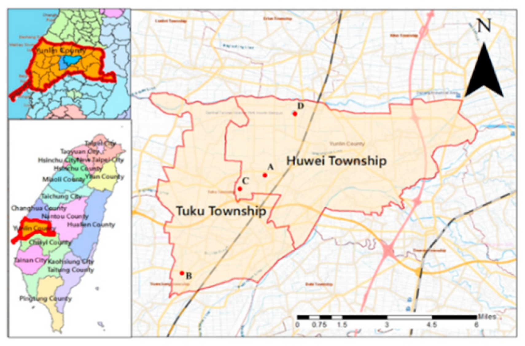
Figure 2.
Spring coefficient versus cyclic no. in A-2 using cyclic triaxial test.
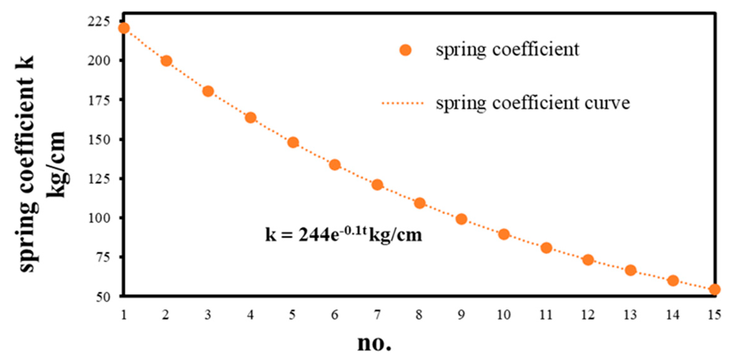
Figure 4.
Damping coefficient versus cyclic no. in A-2 using cyclic triaxial test.
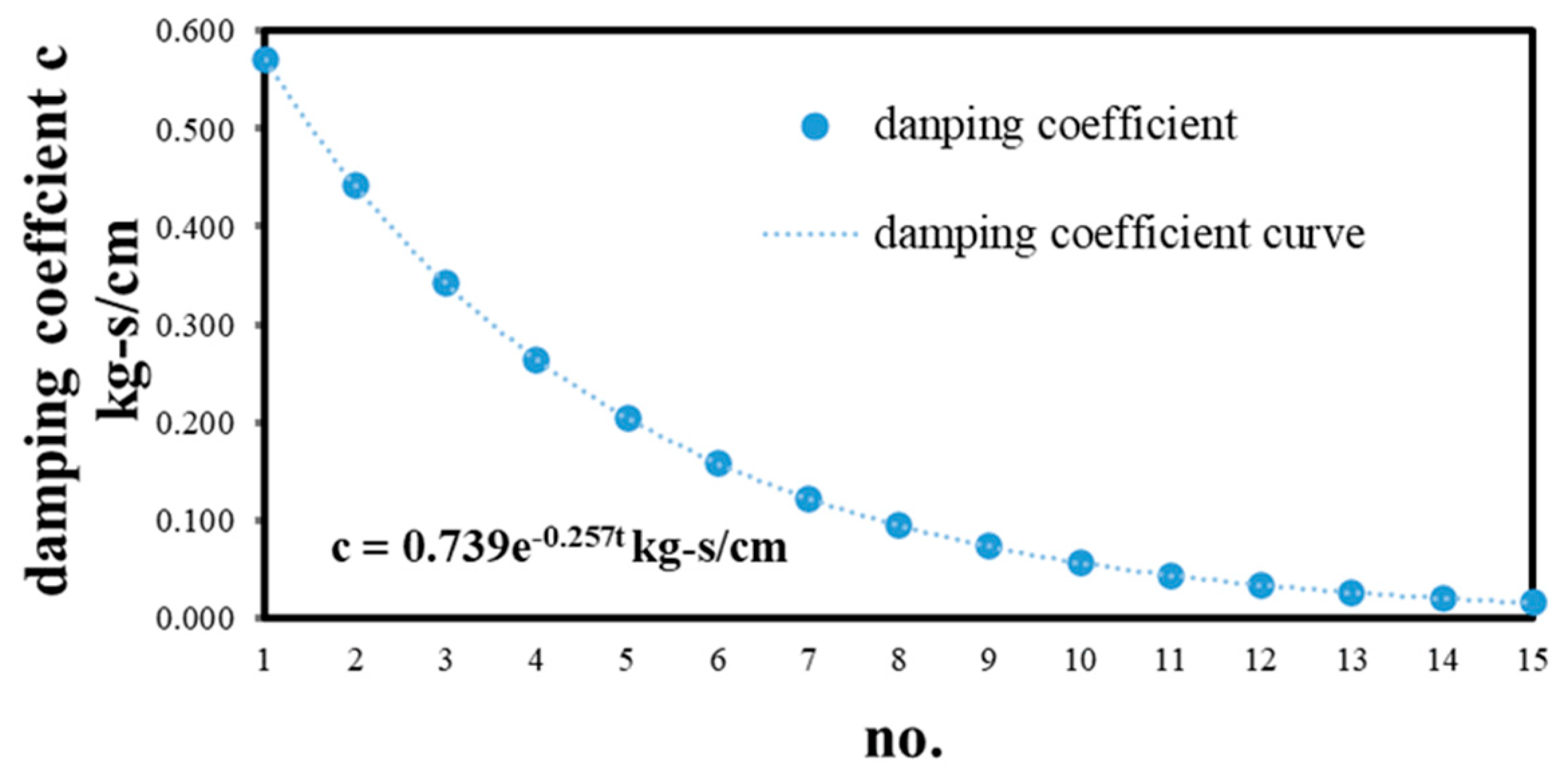
Figure 5.
Numerical results comparison between the Laplace method and Mathematica.
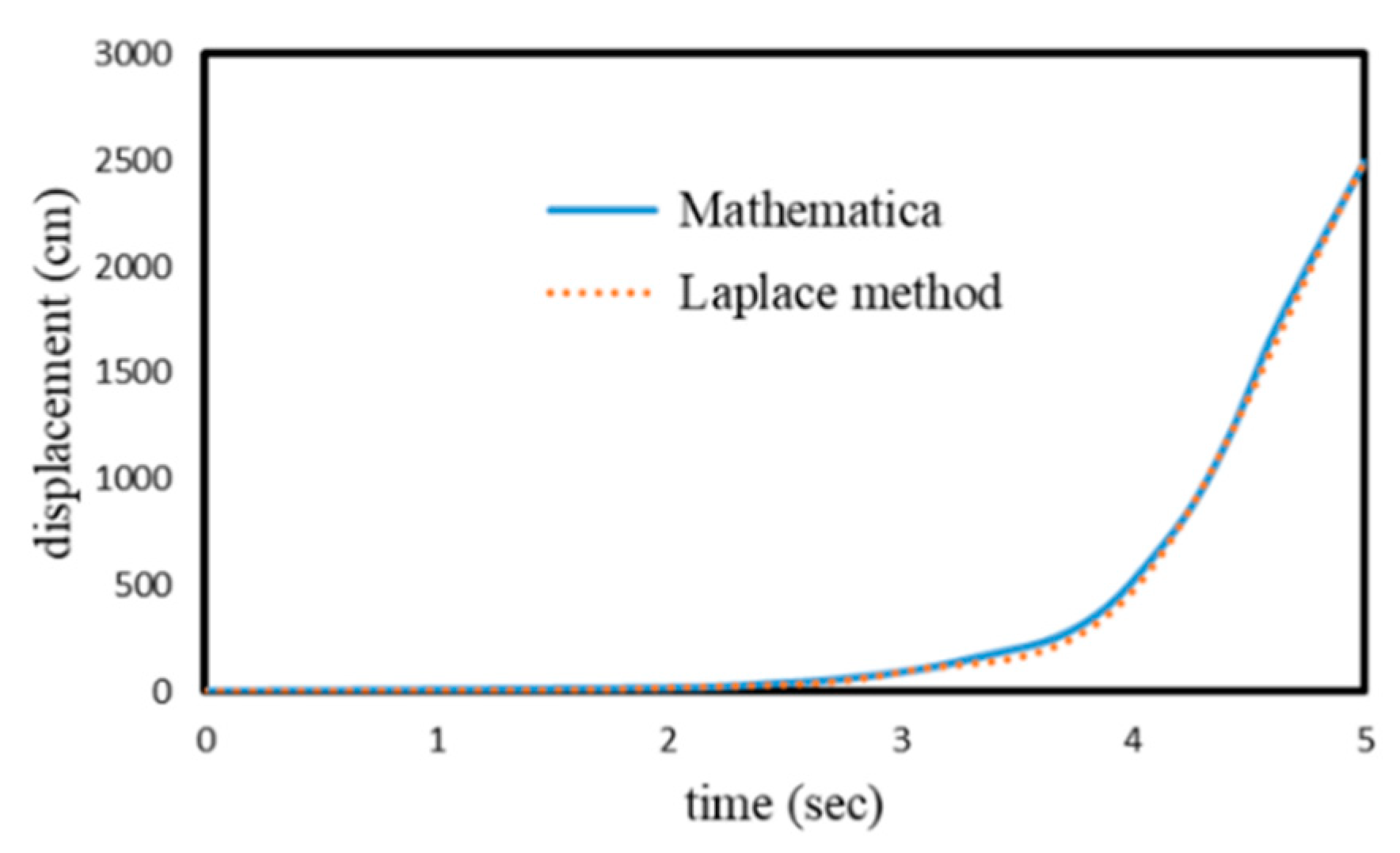
Figure 6.
Strain versus cyclic number for different mass m.
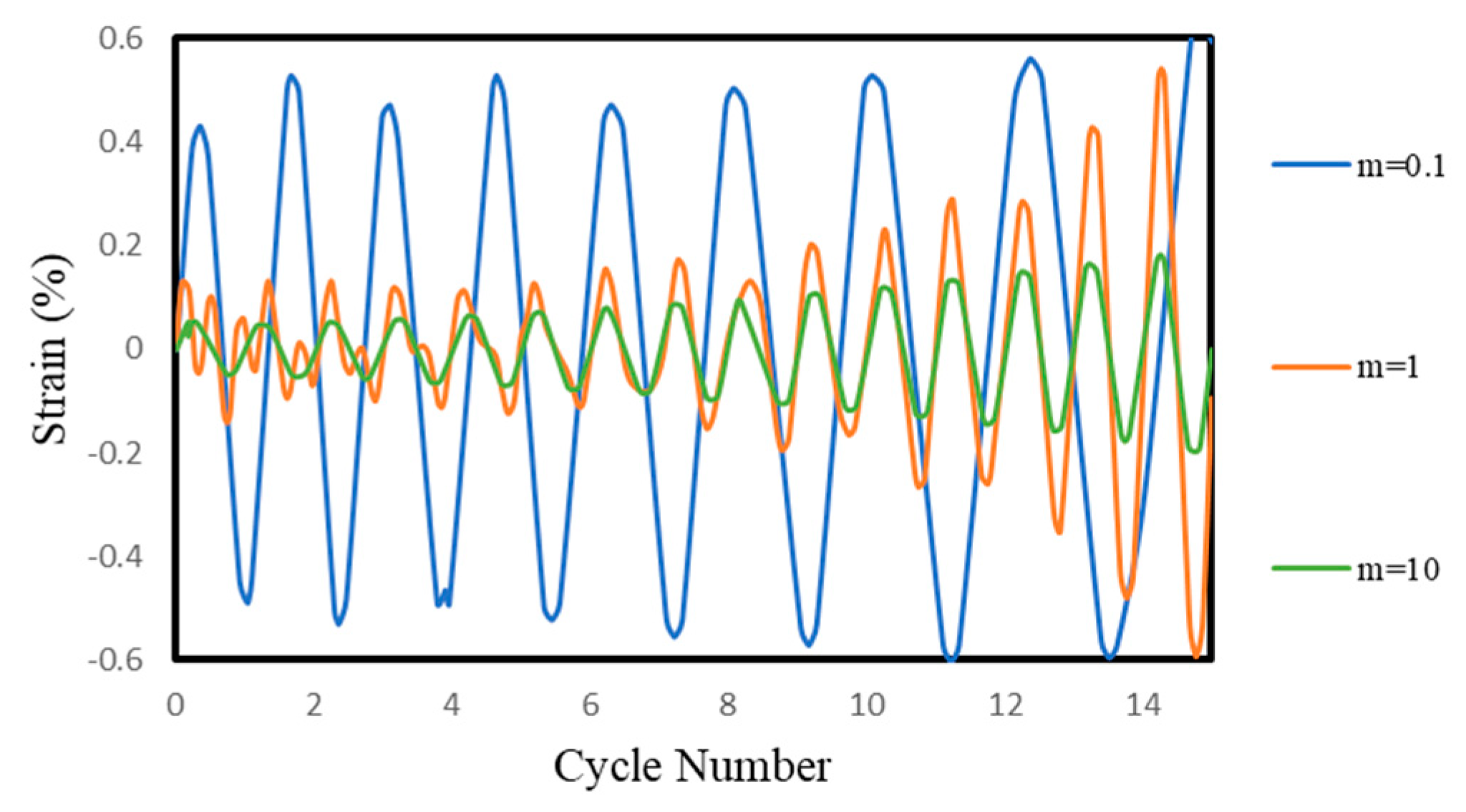
Figure 7.
Strain versus cyclic number for different spring coefficient k.
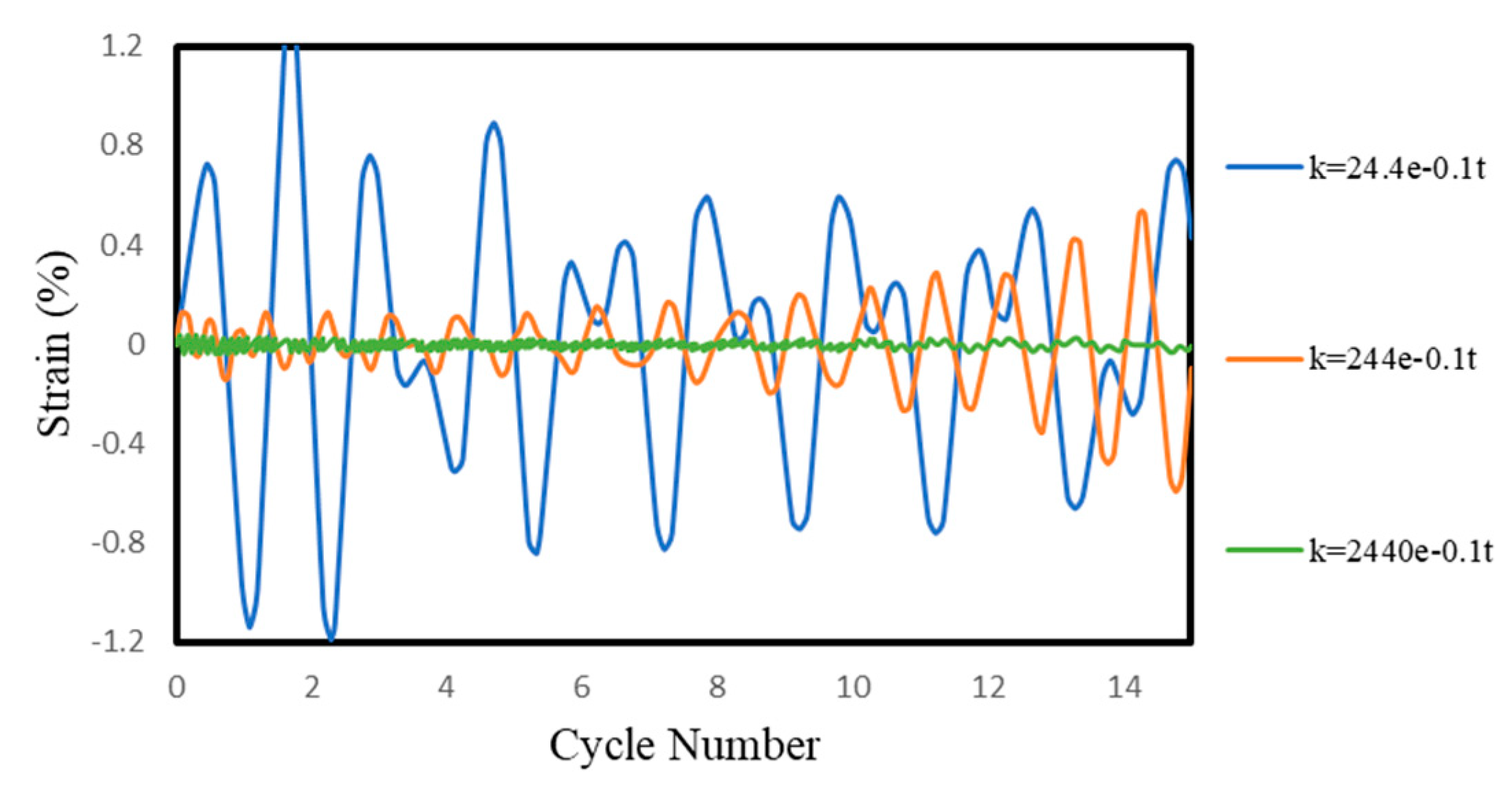
Figure 8.
Strain versus cyclic number for different damping coefficient c.
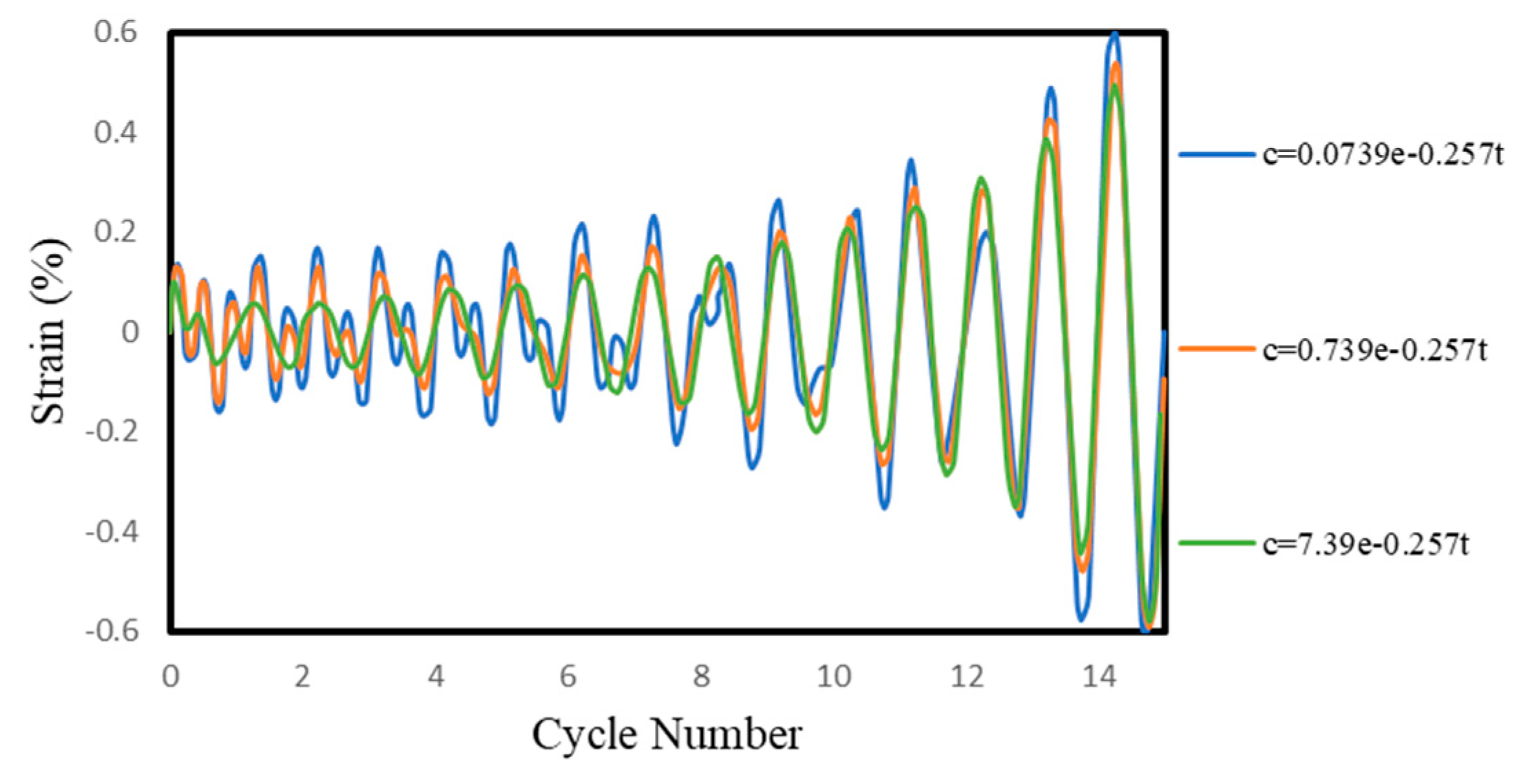
Figure 9.
Strain versus cyclic number for different external force Q0.
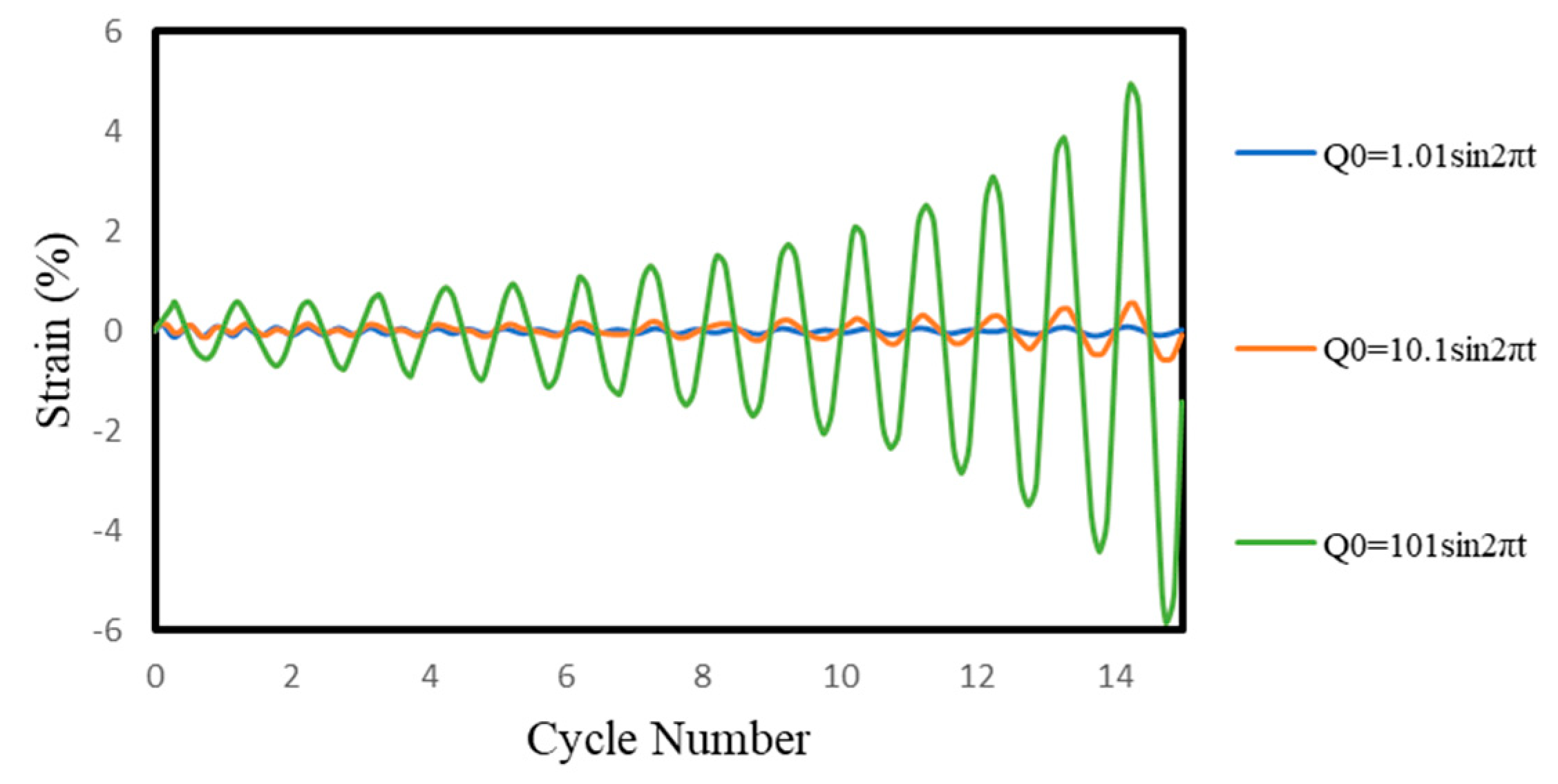
Figure 10.
The results of the cyclic liquefaction triaxial test for the sample at site A.
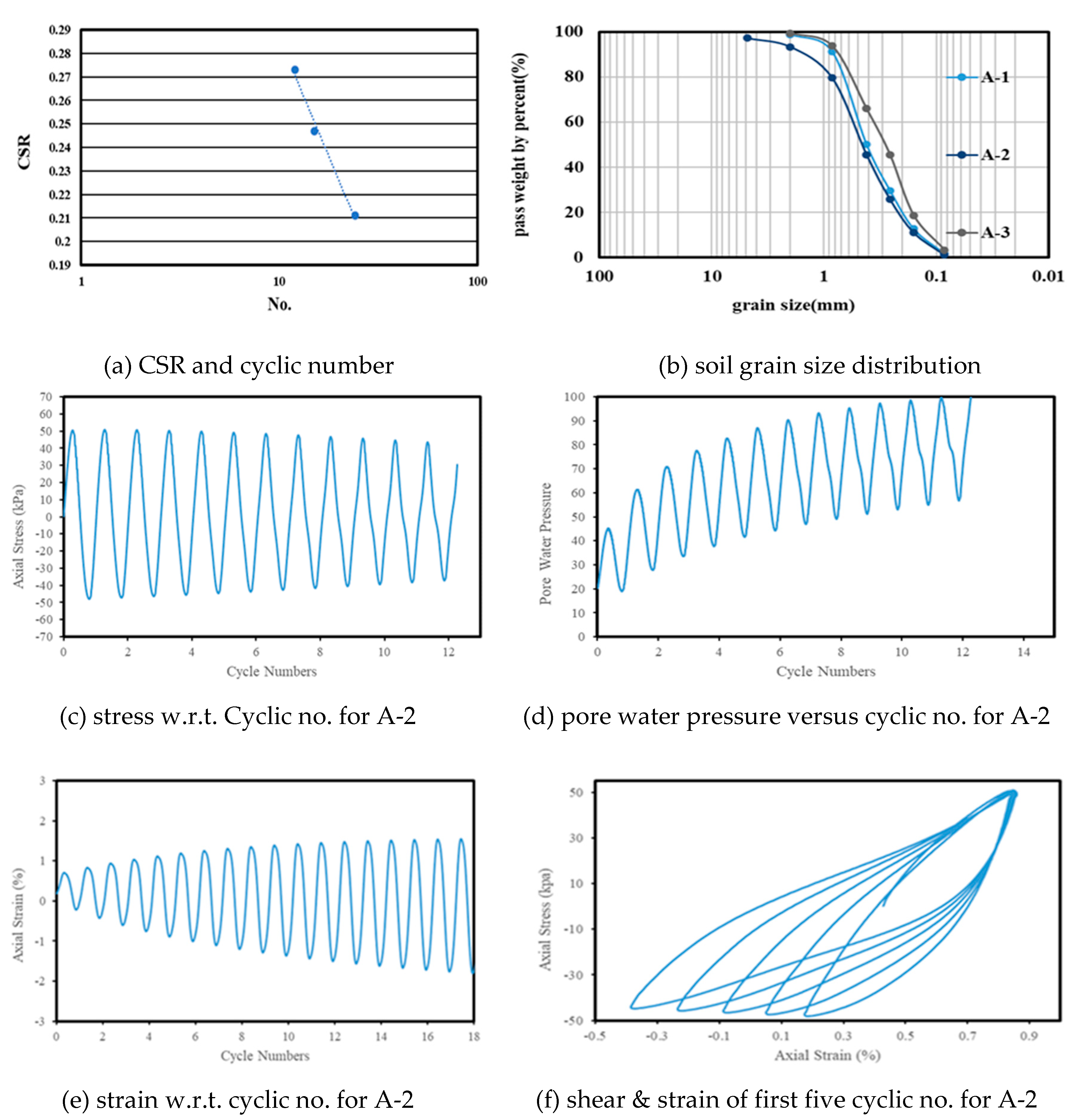
Figure 11.
Comparison of strain and cyclic number between model and experiment for A-2.
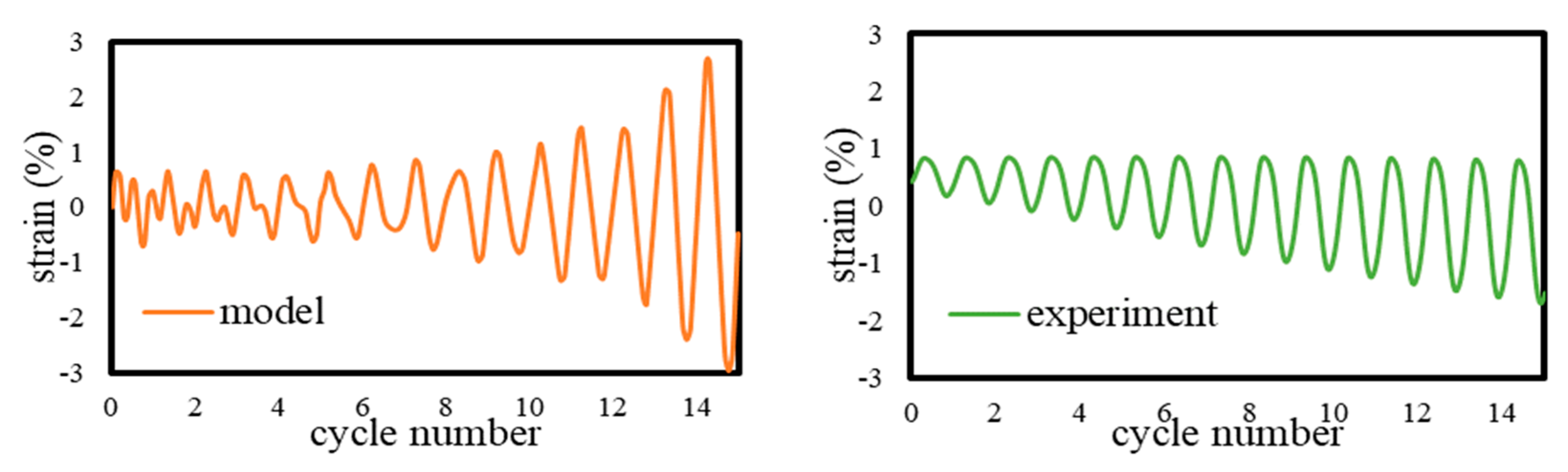
Figure 12.
The results of the cyclic liquefaction triaxial test for the sample at site B.
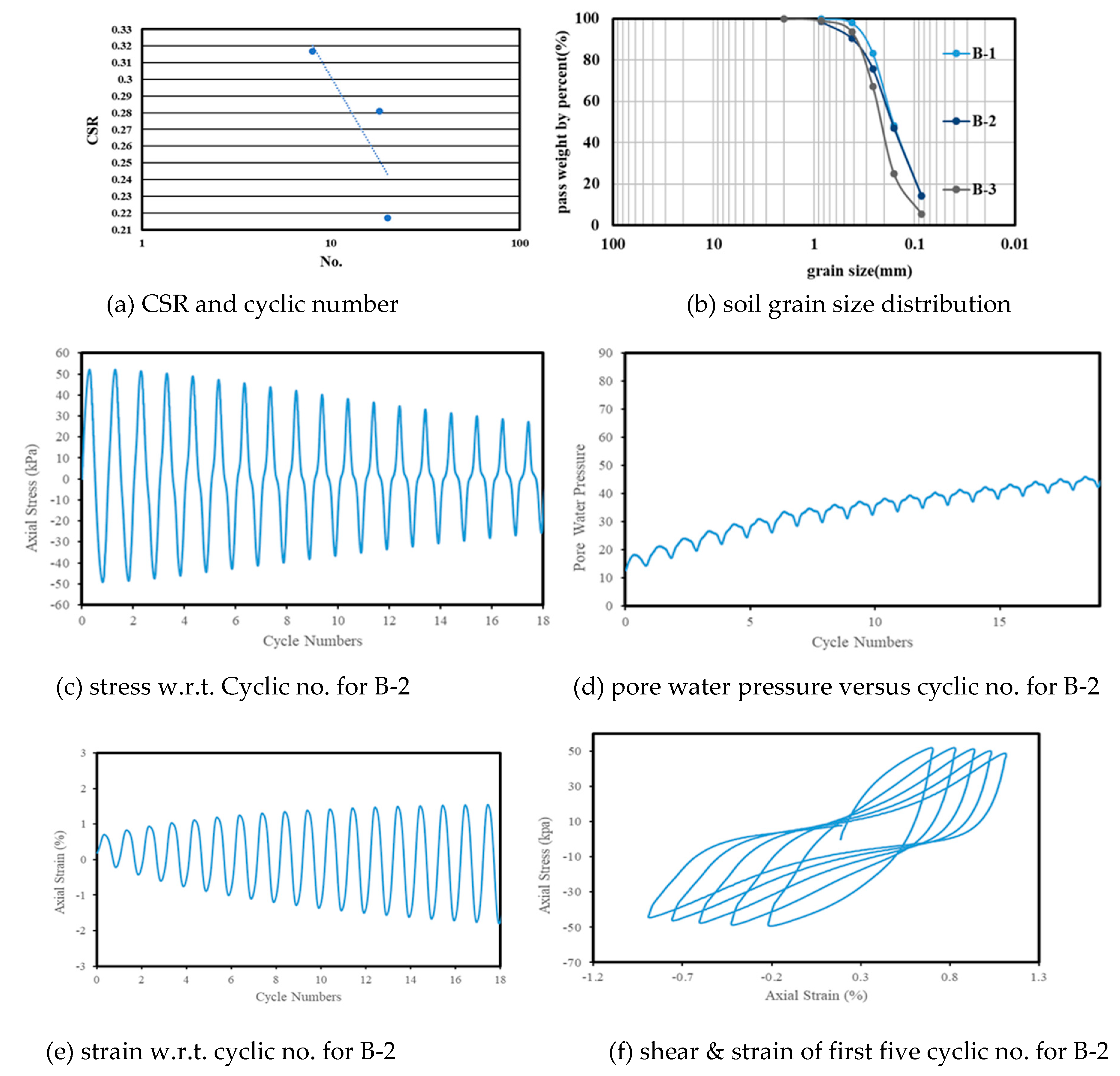
Figure 13.
Comparison of strain and cyclic number between model and experiment for B-2.
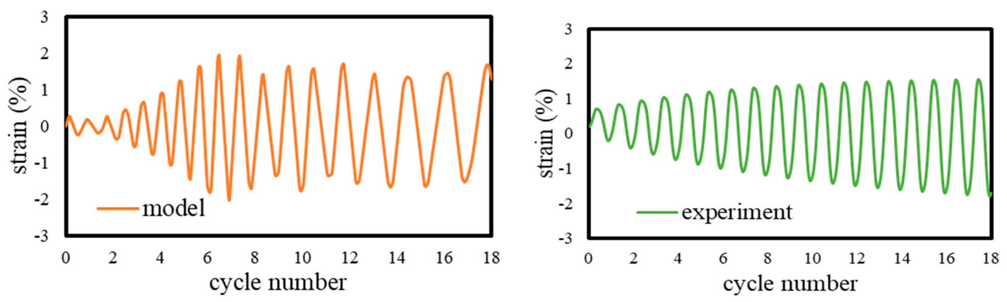
Figure 14.
The results of the cyclic liquefaction triaxial test for the sample at site C.
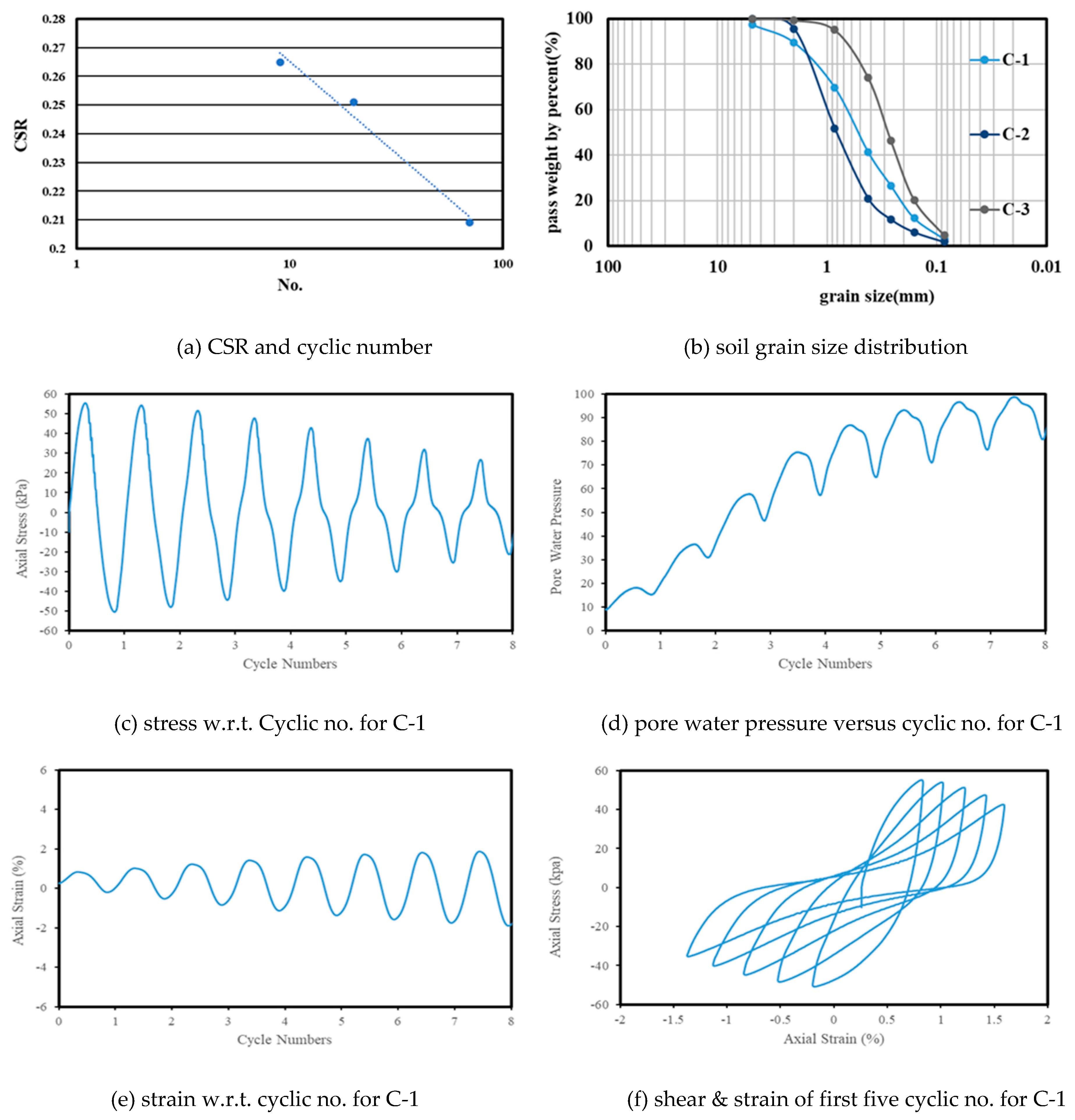
Figure 15.
Comparison of strain and cyclic number between model and experiment for C-1.
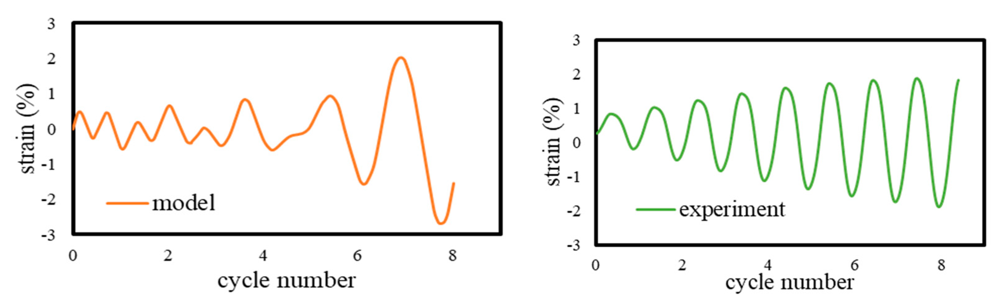
Figure 16.
The results of the cyclic liquefaction triaxial test for the sample at site D.
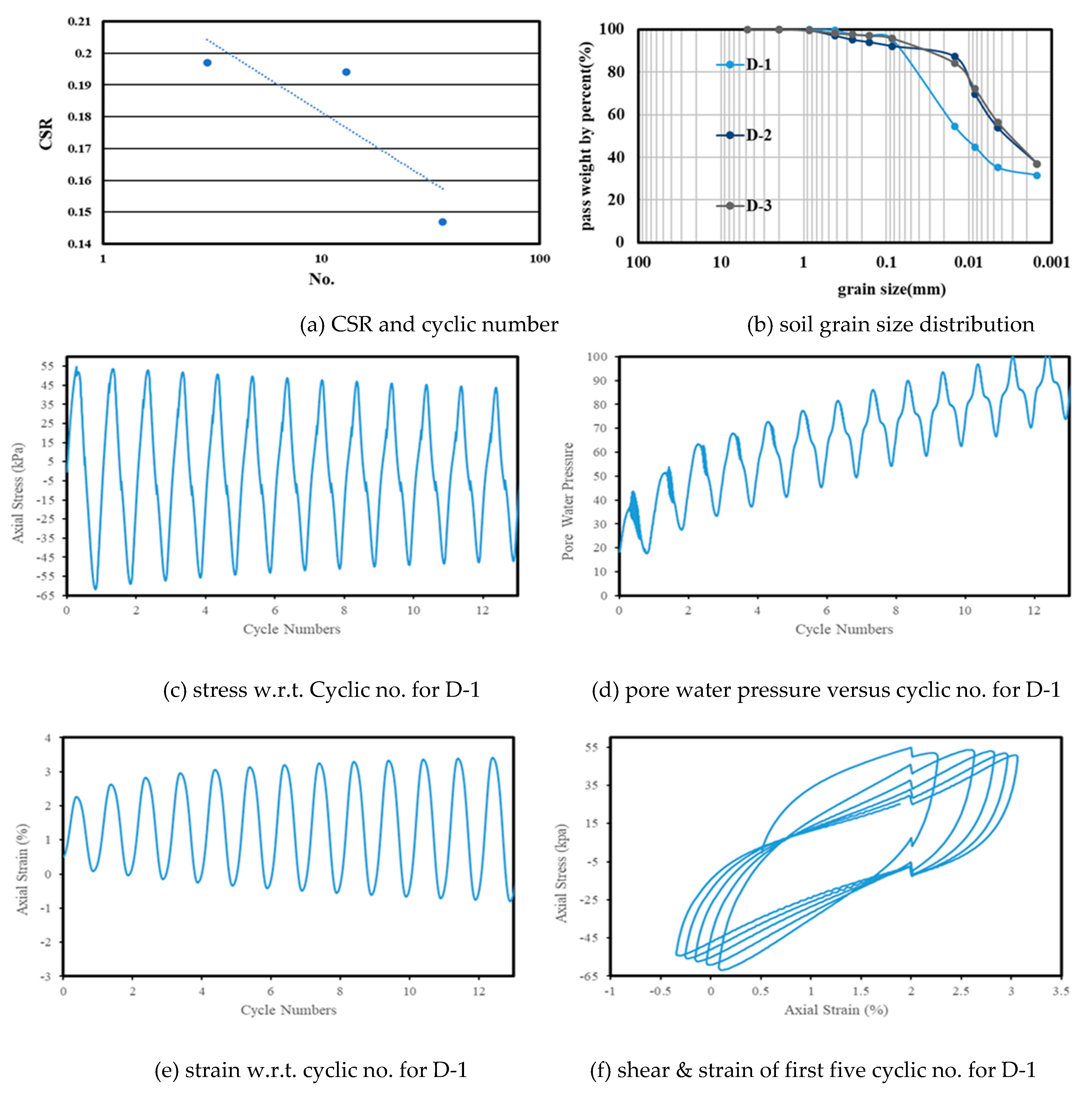
Figure 17.
Comparison of strain and cyclic number between model and experiment for D-1.
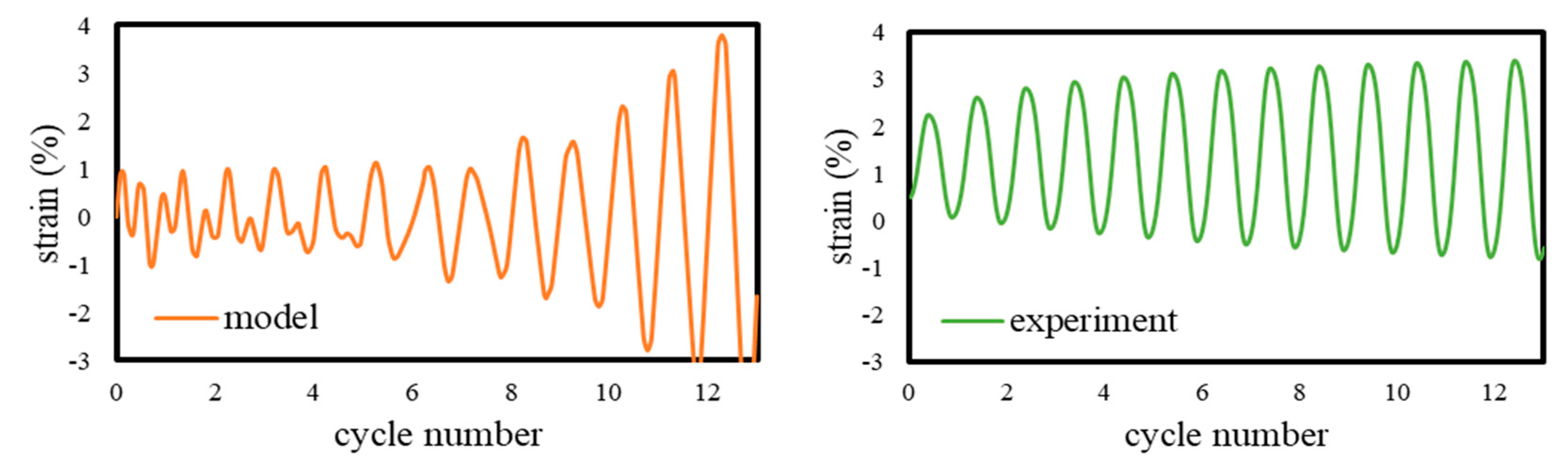

Table 1.
Cyclic triaxial test results of 12 specimens obtained from four sites.
| Specimen No. | B (%) | Soil density (t/m3) | Water content (%) | Gs | Confined pressure σ'c(kPa) | Cyclic stress σdp(kPa) | CSR | Liquefied cyclic no. | CRR7.5 |
|---|---|---|---|---|---|---|---|---|---|
| A-1 | >95 | 2.02 | 16.09 | 2.76 | 100 | 54.51 | 0.273 | 12 | 0.253 |
| A-2 | >95 | 2.02 | 16.09 | 2.76 | 100 | 49.49 | 0.247 | 15 | 0.253 |
| A-3 | >95 | 2.02 | 16.09 | 2.76 | 100 | 42.24 | 0.211 | 24 | 0.253 |
| B-1 | >95 | 2.02 | 22.44 | 2.69 | 90 | 57.10 | 0.317 | 8 | 0.266 |
| B-2 | >95 | 2.02 | 22.44 | 2.69 | 90 | 50.65 | 0.281 | 18 | 0.266 |
| B-3 | >95 | 2.02 | 22.44 | 2.69 | 90 | 39.07 | 0.217 | 20 | 0.266 |
| C-1 | >95 | 2.12 | 23.33 | 2.69 | 100 | 53.02 | 0.265 | 9 | 0.256 |
| C-2 | >95 | 2.12 | 23.33 | 2.69 | 100 | 50.01 | 0.251 | 20 | 0.256 |
| C-3 | >95 | 2.12 | 23.33 | 2.69 | 100 | 41.94 | 0.209 | 70 | 0.256 |
| D-1 | >95 | 1.90 | 37.61 | 2.57 | 150 | 58.25 | 0.194 | 13 | 0.172 |
| D-2 | >95 | 1.90 | 37.61 | 2.57 | 150 | 44.09 | 0.147 | 36 | 0.172 |
| D-3 | >95 | 1.90 | 37.61 | 2.57 | 150 | 59.16 | 0.197 | 3 | 0.172 |
Table 2.
Determine shear modulus using cyclic triaxial test in A-2.
| A-2 | |||||
|---|---|---|---|---|---|
| Cyclic no. | 1 | 2 | 3 | 4 | 5 |
| shear modulus G (kPa) | 5047.94 | 4163.75 | 3478.77 | 2977.94 | 2561.36 |
Table 3.
Determine damping ratio using cyclic triaxial test in A-2.
| A-2 | |||||
|---|---|---|---|---|---|
| Cyclic no. | 1 | 2 | 3 | 4 | 5 |
| damping ratio D | 0.57 | 0.44 | 0.34 | 0.26 | 0.21 |
Table 4.
Parameter range for every parameter.
| m-k-c system | original | reduced | enlarged |
|---|---|---|---|
| Q0 (kg) | 10.1sin2πt | 1.01sin2πt | 101sin2πt |
| k (kgf/cm) | 244e-0.1t | 24.4e-0.1t | 2440e-0.1t |
| m (kg) | 1 | 0.1 | 10 |
| c (kgf-s/cm) | 0.739e-0.257t | 0.0739e-0.257t | 7.39e-0.257t |
Table 5.
The parameter value for different mass m.
| Parameter in m-k-c | value m | ||
|---|---|---|---|
| No. | F1 | F2 | F3 |
| Q0 (kg) | 10.1sin2πt | ||
| k (kgf/cm) | 244e-0.1t | ||
| m (kg) | 1 | 0.1 | 10 |
| c (kgf-s/cm) | 0.739e-0.257t | ||
Table 6.
The parameter value for different spring coefficients, k.
| Parameter in m-k-c | value k | |||
|---|---|---|---|---|
| No. | G1 | G2 | G3 | |
| Q0 (kg) | 10.1 sin2πt | |||
| k (kgf/cm) | 244e-0.1t | 24.4e-0.1t | 2440e-0.1t | |
| m (kg) | 1 | |||
| c (kgf-s/cm) | 0.739e-0.257t | |||
Table 7.
Parameter value for different damping coefficient c.
| Parameter in m-k-c | value c | ||
|---|---|---|---|
| No. | H1 | H2 | H3 |
| Q0 (kg) | 10.1sin2πt | ||
| k (kgf/cm) | 244e-0.1t | ||
| m (kg) | 1 | ||
| c (kgf-s/cm) | 0.739e-0.257t | 0.0739e-0.257t | 7.39e-0.257t |
Table 8.
The parameter value for different external force Q0.
| Parameter in m-k-c | value Q0 | |||
|---|---|---|---|---|
| No. | I1 | I2 | I3 | |
| Q0 (kg) | 10.1sin2πt | 1.01sin2πt | 101sin2πt | |
| k (kgf/cm) | 244e-0.1t | |||
| m (kg) | 1 | |||
| c (kgf-s/cm) | 0.739e-0.257t | |||
Table 9.
Influence degree of each parameter of a mass-spring-damping system.
| parameter | mass (m) | spring coefficient (k) | damping coefficient (c) | external force (Q0) |
|---|---|---|---|---|
| The degree of influence | medium | high | low | high |
Disclaimer/Publisher’s Note: The statements, opinions and data contained in all publications are solely those of the individual author(s) and contributor(s) and not of MDPI and/or the editor(s). MDPI and/or the editor(s) disclaim responsibility for any injury to people or property resulting from any ideas, methods, instructions or products referred to in the content. |
© 2024 by the authors. Licensee MDPI, Basel, Switzerland. This article is an open access article distributed under the terms and conditions of the Creative Commons Attribution (CC BY) license (http://creativecommons.org/licenses/by/4.0/).
Copyright: This open access article is published under a Creative Commons CC BY 4.0 license, which permit the free download, distribution, and reuse, provided that the author and preprint are cited in any reuse.


