Submitted:
04 April 2024
Posted:
04 April 2024
You are already at the latest version
Abstract
The article presents a model for optimizing biomass supply chains using the linear programming framework integrated with a Geographic Information System. Based on the distance from a given type of biomass resource, its calorific value, price, and transportation costs, the model identifies the optimal source of biomass, allowing it to cover the demand for the required total energy value with the lowest possible costs. The case study includes the Połaniec power plant in southeastern Poland and potential sources of forest biomass and agricultural straw within 100 km of the plant. Unit costs of biomass varied depending on biomass availability and energy demands. For energy demand on the level of 1 PJ yearly, the lowest unit costs of biomass (4.08 €/MJ) were when all kinds of biomass were available, and the highest (5.47 €/MJ) was when only stacked wood was available. As energy demand increased, unit costs increased, and the ability to meet this demand with just one type of biomass decreased. The energy biomass sector can utilize the model to benefit both biomass producers and their final buyers.
Keywords:
biomass
; sustainable energy
; costs
; supply chains
; linear programming
; optimization
1. Introduction
Ensuring energy security during climate change has become one of humanity's main challenges. Phasing out fossil fuels and replacing them with renewable energy sources is a central assumption of the EU Energy Policy [1,2]. At the same time, consumers increasingly want clean, renewable, and affordable energy, among others, from biomass sources [3].
In 2020, about 60% of the EU's total renewable energy came from biomass, with forestry biomass accounting for 60% and agricultural biomass and waste accounting for 40% [4]. About half of the woody biomass used for energy production is primary biomass, while the other half is secondary biomass from the timber industry and post-consumer wood. Woody biomass is particularly suitable for energy production due to its high calorific value and relatively low ash content [5]. Wood is the oldest energy source used by humans [6]. Over half of all wood harvested worldwide is used as fuel, supplying about 9% of global primary energy. By depleting stocks of aboveground woody biomass, unsustainable harvesting can contribute to forest degradation, deforestation, and climate change. Management of forests following the principles of sustainable development and the afforestation of new areas has resulted in a steady trend of increasing woody resources in Europe in recent decades. This creates opportunities to use part of the woody biomass from forests for energy but requires proper balancing considering both the needs of the timber industry and ecological requirements [7,8].
The primary source of woody biomass is wood from forests, but the amount of biomass harvested from forests is limited and should be consistent with sustainable forest management. Some of the wood, usually of the lowest quality, is used for energy purposes and is referred to as energy wood. According to Directive 2018/2001 of the European Parliament and the Council of the European Union of 11 December 2018 on the promotion of the use of renewable energy sources [2], energy wood is defined as raw wood material that, due to its qualitative-dimensional and physical-chemical characteristics, has a reduced technical utility value, preventing its industrial use. Logging residues are a significant source of biomass that can be used for energy purposes. The current use of forest residues for commercial and household energy production is small relative to their availability [9].
The assessment of the potential and availability of biomass has been the subject of a relatively large number of studies and scientific publications. Still, for the most part, the results are generalized for large regions, e.g., the world [10] and Europe [11]. They can help shape energy policy while they are of little use to individual biomass users, where transportation distance is a key factor in profitability. The supply and use of woody biomass for Energy in the EU were presented by Panoutsou et al. [12], Bentsen and Felby [13], and Camia et al. [14]. Relatively numerous works show the potential and use of biomass for energy at the national level, including in Sweden [15,16], Germany [17], Czechia [18], and Poland [19,20].
The production of woody biomass and its transport requires some energy input. The energy balance in integrated commercial timber production (saw wood and pulpwood) and energy wood (small dimensions wood and logging residues), considered energy inputs during the whole production cycle and harvesting and transport, was calculated by Routa et al. [21]. The results indicated that the primary energy use incurred during the production cycle is relatively small (less than 3%) compared to the increased potential of energy forest biomass. Winder and Bobar [22] pointed out that the principal use of timber from boreal and temperate forests should be evaluated from a holistic perspective, i.e., it needs to include forest carbon flows related to forest management. They stressed that a scenario where timber is used for 100% energy production is economically unlikely and may create a significant carbon change. In contrast, multiple end-uses are financially feasible and typically achieve far better overall greenhouse gas (GHG) emission reductions. Favero et al. [23,24] discuss wood bioenergy's role in climate mitigation and conclude that the expanded use of wood for bioenergy will result in net carbon benefits. Still, an efficient policy also needs to regulate forest carbon sequestration. The emission benefits of bioenergy compared to the use of fossil fuels are time-dependent [25,26]. All sources of woody bioenergy from sustainably managed forests will produce emission reductions in the long term. Different woody biomass sources have various impacts in the short-medium term. The use of forest residues that are easily decomposable can produce GHG benefits compared to the use of fossil fuels from the beginning of their use. However, the risk of short-to-medium-term negative impacts is high when additional fellings are extracted to produce bioenergy [27].
Optimization methods are widely used for modelling the biomass supply chain for energy purposes [28,29,30]. Methods using geographic information system (GIS) are used to identify the location of bioenergy plants or accurate assessment of transport distances [31,32,33,34]. Linear programming methods are employed for optimizing supply chains of biomass by minimizing costs or maximizing profit [35,36,37,38,39]
The paper aims to develop a model to optimize biomass supply chains for energy employing the linear programming method integrated with a geographic information system (GIS). Based on the distance from a given type of biomass resource, its price and transportation costs, the model identifies the optimal source of woody biomass, allowing it to cover the demand for biomass of a certain total energy value with the lowest possible purchase and transportation costs.
2. Data
The research material consists of the data on the supply, price and transportation costs of forest biomass and straw from agriculture within 100 km of the power plant Połaniec. The power plant uses various types of biomass in addition to coal to produce electricity. Potential sources of biomass were identified within 40 administrative units, hereafter referred to as spatial units. Detailed information about spatial units, the annual supply of different kinds of biomass and the average distance from the power plant are presented in Supplement 1. Data on the availability of woody biomass in spatial units usable for energy purposes comes from [40]. Supply of straw from agriculture was taken as the excess of production over internal consumption of straw in agriculture according to the methodology presented by Gradziuk et al. [41]. Price of biomass comes from [42] while average transportation costs from transport companies operating in the area close to the power plant (information by phone and e-mail). Information about the supply of biomass, its price and transport costs are summarized in Table 1. According to current regulations, large companies can use forest residues (R) and low-quality stacked wood (W) for energy. Firewood is sold only to local individual consumers for households, while better quality wood is sold to the timber industry.
The potential availability of biomass was unevenly distributed across spatial units. Supply of forest biomass depends on the geographic location of the share of forests in a given unit, the species composition and age of forest stands and the intensity of forest management (Figure 1a), while the potential of straw depends on the geographic location, - the share of arable land and the dominant agricultural production profile (Figure 1b).
3. Model Framework
The model concept is presented in the scheme (Figure 2). Input data to the model is information on sources of all biomass potentially usable for technological reasons by the power plant. Each biomass source is treated separately in the model and is described by specifying type (forest residues, solid wood, straw, etc.), quantity (in tons), and distance from the power plant. For a given type of biomass, it is also required to specify its price (€/ton), unit transportation costs (€/ton/km) and calorific value (MJ/ton).
At the model parameterization stage, unit costs are determined for each biomass source, taking into account the purchase of biomass on-site, its transportation to the power plant €/ton), and its energy potential (MJ/ton). The power plant's demand for the total energy value of biomass over a given period (1 year) is also given.
The optimization process uses a linear programming method to minimize the costs of biomass purchase for the given constant demand of biomass energy. The aim can be reversed to maximize biomass energy amount for a given constant biomass purchase budget.
The defined constraints of the model take into account the specifics of a given biomass consumer (the ability to process a particular type of biomass), legal requirements, and biomass potential amount available in spatial units with a known distance from the power plant.
The objective function is defined as follows [44]:
Minimize:
Subject to:
where:
C –total cost of purchasing and transporting biomass,
i – the spatial unit of biomass source,
j – type of biomass,
xij – quantity x of biomass of type j designated for purchase in unit i,
l – distance from power plant to unit i,
E – biomass energy demand by power plant,
γj – calorific value of dry biomass of type j
The amount of energy (Ei) possible to obtain from a specific type and quantity of biomass (Wi) was determined according to the formula:
Ej = Wj·γj
The net calorific value of different kinds of biomass was taken from [43] as follows: 17.5 MJ/kg for solid stacked wood, 13 MJ/kg for chips from forest residues, and 14 MJ/kg for straw from agriculture.
Constraints of the model specify the type of biomass and its potential availability in the area (a certain distance from the power plant), considering the limitations arising from the adopted legal conditions, environmental requirements and competition from other customers.
The amount of a given type of biomass that can be purchased from a given unit is limited by the following inequality:
where: Vijpotential availability of biomass in spatial unit i of type j.
Xij ≤ Vij
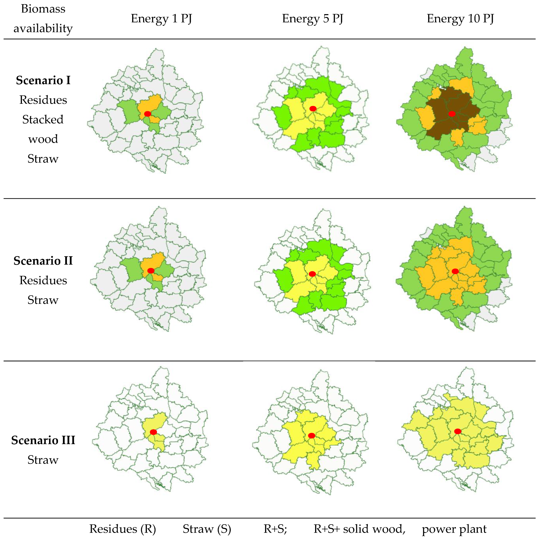
Three scenarios of biomass availability for power plant were distinguished depending on the legal restrictions adopted to allow the use of a particular type of biomass for energy purposes. Scenario 1 - Forest residues, low-quality stacked wood and straw from agriculture are available. Scenario 2 -Forest residues and straw are available. Scenario 3 only has straw from agriculture available. Depending on the energy demand, the following variants were distinguished within each scenario: a) 1 PJ, b) 5 PJ, and c) 10 PJ energy demand, respectively.
All linear programming model calculations were performed using the Gurobi optimizer computer package, version 9.5.1 [45]. Based on the vector layers in the GIS system, the spatial distribution of the analyzed types of biomass was prepared and then, as part of the geolocation process, vector layers was created in which the amount of particular kind of biomass was associated (distance determination) with the biomass consumer – power plant. The source data were integrated into QGis software to generate a layer showing biomass availability's spatial distribution and the final optimising process result[46].
4. Results
The objective function determines the smallest possible sum of the cost of biomass, such as the quantity and type of biomass that will meet the power plant's energy needs. The construction of this function requires incorporating the purchase price, transportation costs and energy value of biomass. Table 2 shows how to enter biomass's purchase and transportation costs into the objective function, while Table 3 shows the incorporation of the energy value of biomass from the selected five spatial units.
The selection of biomass types and sources in the optimization process is done simultaneously. The full notation of the objective function and model constraints for Scenario 1a, taking into account all available types and locations of biomass and biomass energy demand at the level of E= 1PJ ( E = 100000), is presented in Supplement 3. In the case of a fivefold or tenfold increase in energy demand in the formula, only the notation changes to E = 500000 or E = 1000000, respectively. The rest of the formula remains unchanged. The final result of the optimization process with an indication of the smallest possible sum of biomass costs and a detailed list of the type, quantity and spatial unit from which biomass should be purchased according to the assumptions of each scenario is presented in Supplement 4.
The final results of the optimization of biomass supply chains in each scenario are as follows.
Scenario 1. The results of the optimization process for the assumptions: energy demand 1 PJ, all kinds of biomass is available, is illustrated in Table 4 and Figure 2a . To provide this amount of energy, the optimal solution is to purchase 29.70 tons of woody residues from five nearest units (average distance from power plant up to 33 km) and 43.85 tons of straw from two nearest units (distance up to 18 km (Figure2a). Unit costs with this choice of biomass source are at 4.08 Euro/MJ
With an increase in energy demand to 5 PJ, the optimal choice is to purchase 118.14 thousand tons of residues from 18 units with a distance of up to 67 km.) and 247.44 thousand tons of straw from 6 units (up to 39 km) (Figure 2 b). In this case, the unit cost of biomass increases to 4.42 €/MJ (Table 3) due to the need to transport biomass from further locations. Detailed optimization process results for scenarios 1b - 3c are given in Supplement 2.
If the demand is 10 PJ, the optimal choice is to purchase 235.02 thousand tons of residues from 35 units (distance up to 92 km), 476.48 thousand tons of straw from 13 units (up to 57 km) and 16.12 thousand tons of low quality stacked wood (Figure 2c). The unit cost of biomass in this variant is 4.75 E/MJ (Table 5). Its increase is due to both the transport of biomass from further distances and the need to purchase more expensive biomass such as stacked wood.
Scenario 2 biomass of residues and straw is available. The optimization results with the energy demand of 1PJ and 5 PJ are the same as in scenario 1. Despite the availability of stacked, low-quality wood was not selected due to the higher price. On the other hand, with an increase in energy demand to 10 PJ, buying 235.04 thousand tons of residues from 35 units with a distance up to and 496.04 thousand tons of straw from 13 units up to 57 km is optimal. Unit costs in scenario 2c (4.76 €/MJ) are nearly the same as in scenario 1c (4.75€/MJ) - buying straw from further away units was close to buying stacked wood from units near the power plant.
Scenario 3 - only straw is available. To cover the energy demand of 1 PJ, 71.43 tons of straw should be purchased from the three nearest units (located up to 48 km from the power plant (Figure 2d). Unit cost 4.15 €/MJ. Covering the demand for 5 PJ requires purchasing 357.14 thousand tons of straw from nine units (up to 48km), unit cost of 4.57 €/MJ. Covering the demand for 10 PJ requires the purchase of 696.93 thousand tons of straw from 22 units ( up to 78km). For the following energy demands, 1PJ, 5 PJ, and 10 PJ unit costs amounted to 4.15, 4.57, and 5.03 €/MJ, respectively.
Figure 2.
Optimal selection of spatial units for biomass purchase with varying levels of biomass availability and energy demand.
Figure 2.
Optimal selection of spatial units for biomass purchase with varying levels of biomass availability and energy demand.
5. Discussion
In this paper, we developed the model to optimize biomass supply chains for power plant or any end users of biomass for energy production. As inputs, the following data is required: 1) demand for the total calorific value of biomass, 2) indication of the type of biomass usable by the power plant and its calorific value, 3) determination of the quantity and location (distance from the power plant) of each type of biomass, 4) price and transport costs according to types of biomass. As an output, we get the optimal choice of the type, quantity and location of biomass proposed for purchase, providing the required energy at the lowest cost.
The peculiarity of biomass used for energy purposes is characterized by significant geographic variation in supply and price. In our case study, units located to the east of the power plant have a high supply of straw (Lublin province), which is dominated by agricultural areas with high grain production. In contrast, southern and northwestern units have a higher supply of woody biomass (a high proportion of forests) and no surplus straw for energy use. Data on the geographic location of biomass sources was used by Frombo et al. [47] in a developed biomass logistics planning system. Latterini et al. [48] used GIS to estimate the supply chain costs of biomass from olive pruning utilized by a small-size biomass plant.
The developed model simultaneously optimizes biomass's purchase price and transportation costs. In our case study, the cheapest were (without transportation costs) forest residues, straw, and the most expensive stacked wood. Unit transportation costs were different, depending mainly on the volume occupied by a ton of biomass and were lowest for stacked wood, followed by chips from forest residues and highest for straw (0.12, 0.28, and 0.45 €/km/tons, respectively). The model first selected forest residues from units closest to the power plant at low demand. As demand increased, straw from the closest units was selected, while at high demand and the need to reach for biomass much farther away, sacked wood was a more favourable choice than straw.
The effectiveness of small-scale biomass supply chains and different bioenergy production systems utilizing forest residues as biomass sources was conducted by Ahmadi et al. [49]. The authors stated that bioenergy production could be cost-effective in the current carbon credit market. Costs related to the use of wood biomass for energy production on a regional scale were assessed by Furubayashi and Nakata [50]. Our results indicated that unit costs were lowest at low energy demand and increased as demand increased. Findings confirm the results of other studies that it is better to build local small heat plants than large ones that require transporting biomass from farther distances, which, in addition to costs, increases the amount of indirect energy spent and CO2 emissions.
Woody biomass energy potential depends on the available woody biomass resources andhe competition between alternative uses [51]. Lauri et al. [52] stated that woody biomass resources are large enough to cover a substantial share of the world's primary energy consumption in 2050. However, these resources have alternative uses, and their accessibility is limited. Hence, the key question of woody biomass use for energy is not the amount of resources but rather their price.
The greenhouse gas emissions (GHG) performance of different supply-chain configurations of lignocellulosic biomass (stem wood, forest residues, sawmill residues, and sugarcane bagasse) was analyzed by Vera et al. [53]. They found that the use of woody biomass yields better GHG emissions performance for the conversion system than sugarcane bagasse or sugar beets as a result of the higher lignin content. The allocation of biomass resources for minimizing energy system greenhouse gas emissions was studied by Bentsen et al. [54]. They stated that electricity production should be based on forest residues and other woody biomass, heat production on forest and agricultural residues, and liquid fuel production should be based on agricultural residues.
6. Conclusions
The developed model allows the identification of optimal biomass supply chains in terms of economic viability and regulation constraints. Integrating supply chains with geographic information system allows us to trace the legality of biomass sources. The presented methodology can help effectively allocate possible subsidies for renewable energy sources and eliminate cases of inappropriate use, such as direct purchase subsidy to reduce the purchase price - so that better quality wood with a higher free market price instead of to the wood industry can be used by power plants due to subsidies and reduction of the purchase price. The energy biomass sector can utilize the model to benefit both biomass producers and their final buyers.
References
- Moser, C.; Leipold, S. Toward “hardened” accountability? Analyzing the European Union's hybrid transnational governance in timber and biofuel supply chains. Regulation & Governance 2021, 115–132. [Google Scholar] [CrossRef]
- Directive (EU) 2018/2001 on the Promotion of the Use of Energy from Renewable Resources, 2018.
- Richter, D.D.; Jenkins, D.H.; Karakash, J.T.; Knight, J.; McCreery, L.R.; Nemestothy, K.P. Resource policy. Wood energy in America. Science 2009, 323, 1432–1433. [Google Scholar] [CrossRef] [PubMed]
- Chudy, R.; Szulecki, K.; Siry, J.; Grala, R. Biomasa drzewna jako surowiec dla energetyki. Academia 2021, 62–65. [Google Scholar] [CrossRef]
- McKendry, P. Energy production from biomass (part 1): overview of biomass. Bioresource Technology 2002, 83, 37–46. [Google Scholar] [CrossRef] [PubMed]
- Bailis. The carbon footprint of traditional woodfuels 2015. [CrossRef]
- Verkerk, P.J.; Anttila, P.; Eggers, J.; Lindner, M.; Asikainen, A. The realisable potential supply of woody biomass from forests in the European Union. Forest Ecology and Management 2011, 261, 2007–2015. [Google Scholar] [CrossRef]
- Banaś, J.; Utnik-Banaś, K. Using Timber as a Renewable Resource for Energy Production in Sustainable Forest Management. Energies 2022, 15, 2264. [Google Scholar] [CrossRef]
- Durocher, C.; Thiffault, E.; Achim, A.; Auty, D.; Barrette, J. Untapped volume of surplus forest growth as feedstock for bioenergy. Biomass and Bioenergy 2019, 120, 376–386. [Google Scholar] [CrossRef]
- Smeets, E.M.W.; Faaij, A.P.C. Bioenergy potentials from forestry in 2050. Climatic Change 2007, 81, 353–390. [Google Scholar] [CrossRef]
- Karjalainen, T.; Asikainen, A.; Ilavsky, J.; Zamboni, R.; Hotari, K.-E.; Röser, D. Estimation of energy wood potential in Europe 2004. 2004. [Google Scholar]
- Panoutsou, C.; Eleftheriadis, J.; Nikolaou, A. Biomass supply in EU27 from 2010 to 2030. Energy Policy 2009, 37, 5675–5686. [Google Scholar] [CrossRef]
- Bentsen, N.S.; Felby, C. Biomass for energy in the European Union - a review of bioenery resource assessment. Biotechnology for Biofuels 2012, 1–10. [Google Scholar]
- Camia, A.; Giuntoli, J.; Jonsson, R.; Robert, N.; Cazzaniga, N.E.; Jasinevičius, G.; Grassi, G.; Barredo, J.I.; Mubareka, S. The use of woody biomass for energy production in the EU; JRC science for policy report JRC122719, Luxembourg, 2021.
- Lundmark, R.; Athanassiadis, D.; Wetterlund, E. Supply assessment of forest biomass – A bottom-up approach for Sweden. Biomass and Bioenergy 2015, 75, 213–226. [Google Scholar] [CrossRef]
- Kumar, A.; Adamopoulos, S.; Jones, D.; Amiandamhen, S.O. Forest Biomass Availability and Utilization Potential in Sweden: A Review. Waste Biomass Valor 2021, 12, 65–80. [Google Scholar] [CrossRef]
- Ralf-Uwe, S.; Tran Thuc, H.; Karsten, G.; Suili, X.; Wolfgang, W. Residential Heating Using Woody Biomass in Germany—Supply, Demand, and Spatial Implications. Land 2022. [Google Scholar] [CrossRef]
- Šafařík, D.; Hlaváčková, P.; Michal, J. Potential of Forest Biomass Resources for Renewable Energy Production in the Czech Republic. Energies 2022, 15, 47. [Google Scholar] [CrossRef]
- Różański, H.; Jabłoński, K. Możliwości pozyskania biomasy leśnej na cele energetyczne w Polsce. JOURNAL OF CIVIL ENGINEERING, ENVIRONMENT AND ARCHITECTURE 2015, 351–358. [Google Scholar] [CrossRef]
- Majchrzak, M.; Szczypa, P.; Adamowicz, K. Supply of Wood Biomass in Poland in Terms of Extraordinary Threat and Energy Transition. Energies 2022. [Google Scholar] [CrossRef]
- Routa, J.; Kellomäki, S.; Kilpeläinen, A.; Peltola, H.; Strandman, H. Effects of forest management on the carbon dioxide emissions of wood energy in integrated production of timber and energy biomass. GCB Bioenergy 2011, 3, 483–497. [Google Scholar] [CrossRef]
- Winder, G.M.; Bobar, A. Responses to stimulate substitution and cascade use of wood within a wood use system: Experience from Bavaria, Germany. Applied Geography 2018, 90, 350–359. [Google Scholar] [CrossRef]
- Favero, A.; Daigneault, A.; Sohngen, B. Forests: Carbon sequestration, biomass energy, or both? Sci. Adv. 2020, 1–13. [Google Scholar] [CrossRef] [PubMed]
- Favero, A.; Mendelsohn, R.; Sohngen, B. Using forests for climate mitigation: sequester carbon or produce woody biomass? Climatic Change 2017, 195–206. [Google Scholar] [CrossRef]
- Ameray, A.; Bergeron, Y.; Valeria, O.; Montoro Girona, M.; Cavard, X. Forest Carbon Management: a Review of Silvicultural Practices and Management Strategies Across Boreal, Temperate and Tropical Forests. Curr Forestry Rep 2021, 7, 245–266. [Google Scholar] [CrossRef]
- Baral, A.; Malins, C. Assessing the climate mitigation potential of biofuels derived from residues and wastes in the European context 2014.
- Giuliana, Z.; Naomi, P. Neil Bird. Is woody bioenergy carbon neutral? A comparative assessment of emissions from consumption of woody bioenergy and fossil fuel. Bioenergy 2012, 761–772. [Google Scholar] [CrossRef]
- Abusaq, Z.; Habib, M.S.; Shehzad, A.; Kanan, M.; Assaf, R. A Flexible Robust Possibilistic Programming Approach toward Wood Pellets Supply Chain Network Design. Mathematics 2022, 10. [Google Scholar] [CrossRef]
- Keith, K.; Castillo-Villar, K.K. Stochastic Programming Model Integrating Pyrolysis Byproducts in the Design of Bioenergy Supply Chains. Energies 2023, 16. [Google Scholar] [CrossRef]
- Batista, R.M.; Converti, A.; Pappalardo, J.; Benachour, M.; Sarubbo, L.A. Tools for Optimization of Biomass-to-Energy Conversion Processes. Processes 2023, 11. [Google Scholar] [CrossRef]
- Zyadin, A.; Natarajan, K.; Latva-Käyrä, P.; Igliński, B.; Iglińska Anna; Trishkin, M. ; Pelkonen, P.; Pappinen Ari. Estimation of surplus biomass potential in southern and central Poland using GIS applications. Renewable and Sustainable Energy Reviews 2018, 89, 204–215. [Google Scholar] [CrossRef]
- Wang, Y.; Wang, J.; Schuler, J.; Hartley, D.; Volk, T.; Eisenbies, M. Optimization of harvest and logistics for multiple lignocellulosic biomass feedstocks in the northeastern United States. Energy 2020, 197, 117260. [Google Scholar] [CrossRef]
- Sahoo, K.; Hawkins, G.L.; Yao, X.A.; Samples, K.; Mani, S. GIS-based biomass assessment and supply logistics system for a sustainable biorefinery: A case study with cotton stalks in the Southeastern US. Applied Energy 2016, 182, 260–273. [Google Scholar] [CrossRef]
- Lozano-García, D.F.; Santibañez-Aguilar, J.E.; Lozano, F.J.; Flores-Tlacuahuac, A. GIS-based modeling of residual biomass availability for energy and production in Mexico. Renewable and Sustainable Energy Reviews 2020, 120, 109610. [Google Scholar] [CrossRef]
- Reis, S.A.d.; Leal, J.E.; Thomé, A.M.T. A Two-Stage Stochastic Linear Programming Model for Tactical Planning in the Soybean Supply Chain. Logistics 2023, 7. [Google Scholar] [CrossRef]
- Ferretti, I. Optimization of the Use of Biomass Residues in the Poplar Plywood Sector. Procedia Computer Science 2021, 180, 714–723. [Google Scholar] [CrossRef]
- Abdelhady, S.; Shalaby, M.A.; Shaban, A. Techno-Economic Analysis for the Optimal Design of a National Network of Agro-Energy Biomass Power Plants in Egypt. Energies 2021, 14. [Google Scholar] [CrossRef]
- Nienow, S.; McNamara, K.T.; Gillespie, A.R. Assessing plantation biomass for co-firing with coal in northern Indiana: A linear programming approach. Biomass and Bioenergy 2000, 18, 125–135. [Google Scholar] [CrossRef]
- Wu, J.; Zhang, J.; Yi, W.; Cai, H.; Li, Y.; Su, Z. Agri-biomass supply chain optimization in north China: Model development and application. Energy 2022, 239, 122374. [Google Scholar] [CrossRef]
- Forest Data Bank. Available online: www.bdl.lasy.gov.pl/portal/en (accessed on 20 January 2024).
- Gradziuk, P.; Gradziuk, B.; Trocewicz, A.; Jendrzejewski, B. Potential of Straw for Energy Purposes in Poland—Forecasts Based on Trend and Causal Models. Energies 2020, 13, 5054. [Google Scholar] [CrossRef]
- State Forests. Information on Sales of Selected Groups of Wood in Forest Districts State Forests. Available online: https://drewno.zilp.lasy.gov.pl/drewno/ (accessed on 15 February 2024).
- Günther, B.; Gebauer, K.; Barkowski, R.; Rosenthal, M.; Bues, C.-T. Calorific value of selected wood species and wood products. Eur. J. Wood Prod. 2012, 70, 755–757. [Google Scholar] [CrossRef]
- Bettinger, P.; Boston, K. ; Siry, Jacek, P; Grebner, Donald, L. Forest Management and Planning: Linear Programming, Ed.; Elsevier: San Diego, California, USA, 2009. [Google Scholar]
- Gurobi Optimizer; Gurobi Optimization, 2023.
- QGIS Geographic Information System. QGIS Association.; QGIS.org., 2024.
- Frombo, F.; Minciardi, R.; Robba, M.; Rosso, F.; Sacile, R. Planning woody biomass logistics for energy production: A strategic decision model. Biomass and Bioenergy 2009, 33, 372–383. [Google Scholar] [CrossRef]
- Latterini, F.; Stefanoni, W.; Suardi, A.; Alfano, V.; Bergonzoli, S.; Palmieri, N.; Pari, L. A GIS Approach to Locate a Small Size Biomass Plant Powered by Olive Pruning and to Estimate Supply Chain Costs. Energies 2020, 13, 3385. [Google Scholar] [CrossRef]
- Ahmadi, L.; Kannangara, M.; Bensebaa, F. Cost-effectiveness of small scale biomass supply chain and bioenergy production systems in carbon credit markets: A life cycle perspective. Sustainable Energy Technologies and Assessments 2020, 37, 100627. [Google Scholar] [CrossRef]
- Furubayashi, T.; Nakata, T. Analysis of woody biomass utilization for heat, electricity, and CHP in a regional city of Japan. Journal of Cleaner Production 2021, 290, 125665. [Google Scholar] [CrossRef]
- Berndes. [CrossRef]
- Lauri, P.; Havlík, P.; Kindermann, G.; Forsell, N.; Böttcher, H.; Obersteiner, M. Woody biomass energy potential in 2050. Energy Policy 2014, 66, 19–31. [Google Scholar] [CrossRef]
- Vera, I.; Hoefnagels, R.; van der Kooij, A.; Moretti, C.; Junginger, M. A carbon footprint assessment of multi-output biorefineries with international biomass supply: a case study for the Netherlands. Biofuels, Bioprod. Bioref. 2020; 198–224. [Google Scholar] [CrossRef]
- Bentsen, N.S.; Jack, M.W.; Felby, C.; Thorsen, B.J. Allocation of biomass resources for minimising energy system greenhouse gas emissions. Energy 2014, 69, 506–515. [Google Scholar] [CrossRef]
Figure 1.
The potential availability of forest biomass and straw from agriculture for energy production.
Figure 1.
The potential availability of forest biomass and straw from agriculture for energy production.
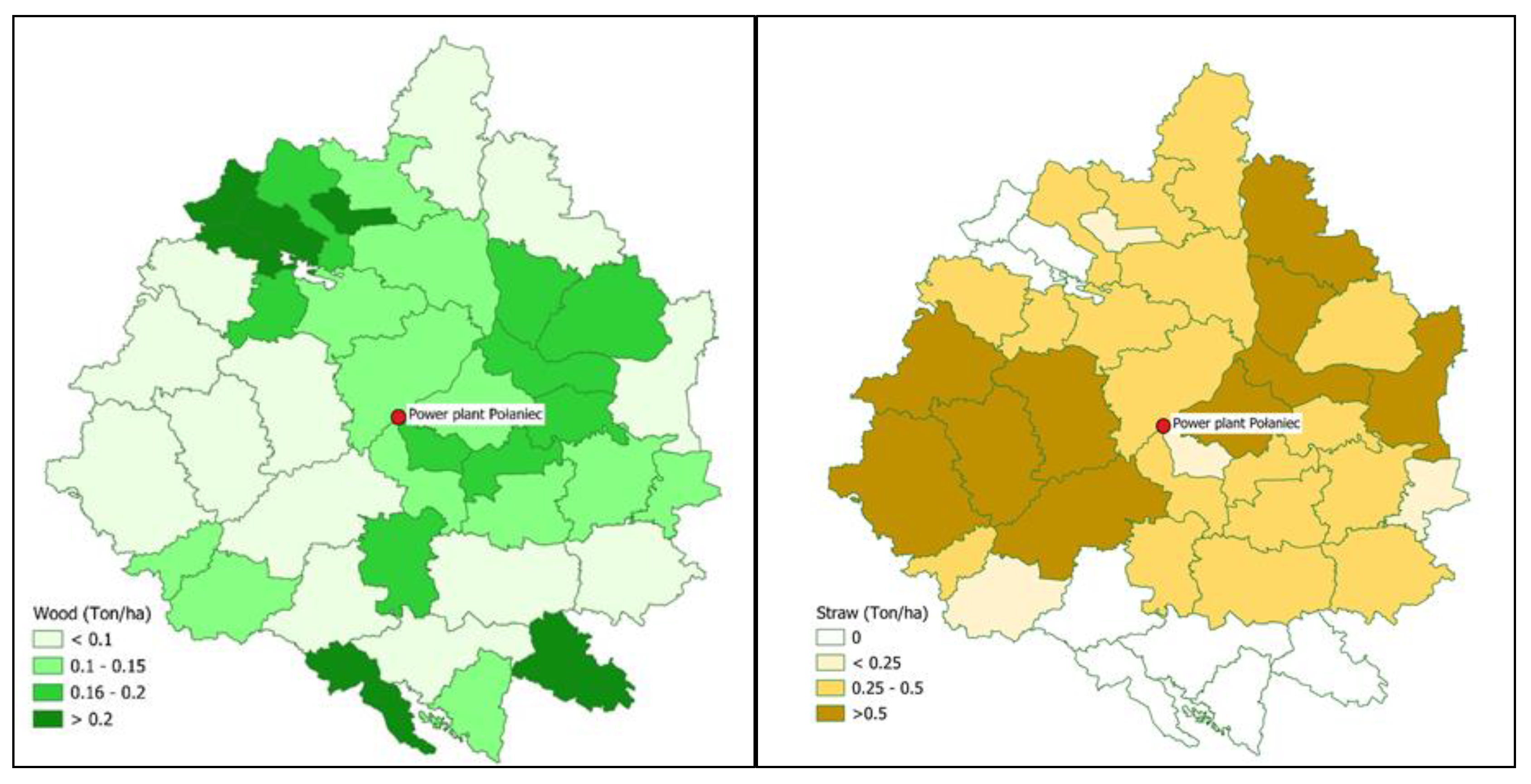
Figure 2.
Conceptual diagram of the biomass supply chains optimization model.
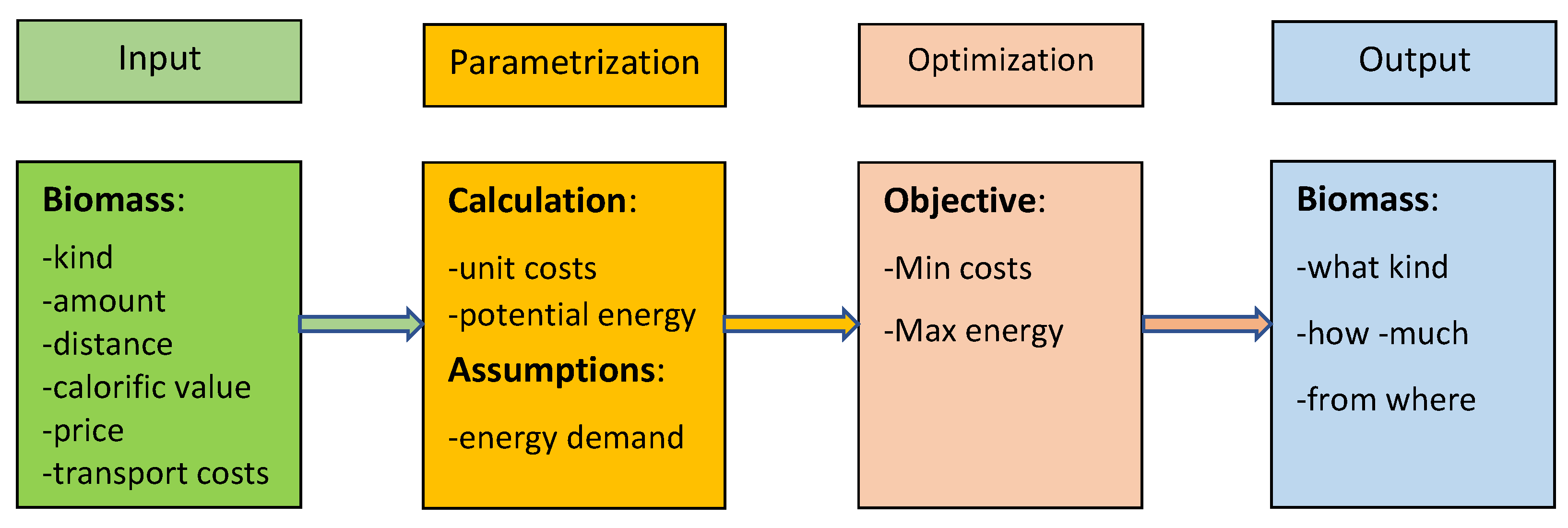

Table 1.
Potential yearly supply and price of different kinds of biomass.
| Biomass assortment | Supply availability (thousand tons) |
Price (€/tons) |
Transport cost (€/km/tons) |
| Forest residues | 265.98 | 44.20 | 0.28 |
| Low-quality stacked wood | 102.70 | 87.80 | 0.12 |
| Straw from agriculture | 1322.19 | 50.56 | 0.45 |
Table 2.
Potential Costs of purchasing and transporting biomass from the five spatial units closest to the power plant.
Table 2.
Potential Costs of purchasing and transporting biomass from the five spatial units closest to the power plant.
| Spatial Unit | Distance | Potential costs of purchase | ||
| Residues | Stacked wood | Straw | ||
| Mielec | 16 | 44.21) X1,1 + 0.282) ·16 X1,1 | 87.83) X1,2 + 0.124) ·16 X1,2 | 50.565) X1,3 +) ·16 X1,3 |
| Staszów | 18 | 44.2 X2,1 + 5.04 X2,1 | 87.8 X2,2 + 2.16 X2,2 | 50.56 X2,3 + 8.1 X2,3 |
| Tuszyma | 24 | 44.2 X3,1 + 6.72 X3,1 | 87.8 X3,2 + 2.88 X3,2 | 50.56 X3,3 + 10.8 X3,3 |
| N. Dęba | 30 | 44.2 X4,1 + 8.4 X4,1 | 87.8 X4,2 + 3.6 X4,2 | 50.56 X4,3 + 13.5 X4,3 |
| Chmielnik | 33 | 44.2 X5,1 + 9.24 X5,1 | 87.8 X5,2 + 3.96 X5,2 | 50.56 X5,3 + 14.85 X5,3 |
1) – residues price (€/ton); 2) – unit transport costs of residues (€/ton/km); 3)- stacked wood price; 4) -unit transport costs of staked wood; 5)straw price; 6) unit transport costs of straw; Xi,j- amount of j kind biomass from unit i, for residues j=1, for stacked wood j=2, for straw j=3.
Table 3.
Potential energy value and maximum available amount of biomass from five spatial units of the nearest power plants.
Table 3.
Potential energy value and maximum available amount of biomass from five spatial units of the nearest power plants.
| Spatial units | Potential Energy value (TJ) | Maximal available biomass (tons 103) | ||||
| Residues | Stacked Wood | Straw | Residues | Stacked Wood | Straw | |
| Mielec | 131) X1,1 | 17.52) X1,2 | 143) X1,3 | X1,1 ≤ 3.29 | X1,2 ≤ 1.12 | X1,3 ≤.6.42 |
| Staszów | 13 X2,1 | 17.5 X2,2 | 14 X2,3 | X2,1 ≤ 9.21 | X2,2 ≤ 3.54 | X2,3 ≤ 60.45 |
| Tuszyma | 13 X3,1 | 17.5 X3,2 | 14 X3,3 | X3,1 ≤ 5.47 | X3,2 ≤ 1.93 | X3,3 ≤ 14.32 |
| N. Deba | 13 X4,1 | 17.5 X4,2 | 14 X4,3 | X4,1 ≤ 7.25 | X4,2 ≤ 2.59 | X4,3 ≤ 54.58 |
| Chmielnik | 13 X5,1 | 17.5 X5,2 | 14 X5,3 | X5,1 ≤ 4.48 | X5,2 ≤ 1.62 | X5,3 ≤ 74.88 |
calorific value of: 1) residues, 2) stacked wood, 3) straw.
Table 4.
Detailed results of biomass supply chains optimization for scenario 1a.
| Spatial unit | Average distance (km) | Demand for biomass (thousand tons) | Energy (TJ) | Cost (thousand €) | |||
| Rezidues | Straw | Rezidues | Straw | Rezidues | Straw | ||
| Mielec | 16 | 3.29 | 6.42 | 42.76 | 89.88 | 160.11 | 370.82 |
| Staszów | 18 | 9.21 | 37.43 | 119.76 | 523.98 | 453.60 | 2195.47 |
| Tuszyma | 24 | 5.47 | - | 71.15 | - | 278.68 | - |
| Nowa Dęba | 30 | 7.25 | - | 94.26 | - | 381.40 | - |
| Chmielnik | 33 | 4.48 | - | 58.21 | - | 239.30 | - |
| Total | 29.70 | 43.85 | 386.14 | 613.86 | 1513.09 | 2566.29 | |
| 73.55 | 1000 | 4079.38 | |||||
Constraints: energy demand = 1 PJ; biomass availability: forest residues, low-quality wood, straw from agriculture.
Table 5.
Demand and unit costs in different biomass availability.
| Biomass | Biomass demand (thousand tons) | Unit costs €/MJ | ||||
| 1 PJ (a) | 5 PJ (b) | 10 PJ (c) | a | b | c | |
| Forest residues (R) | 76.92 | in. | in. | 4.18 | in. | in. |
| Stacked wood (W) | 58.82 | in. | in. | 5.47 | in. | in. |
| Straw (S) | 71.43 | 357.14 | 714.29 | 4.15 | 4.57 | 5.03 |
| R +W | 76.92 | 356.70 | in. | 4.18 | 5.05 | in. |
| R+S | 73,55 | 365.58 | 731.07 | 4.03 | 4.42 | 4.76 |
| R+W+S | 73.55 | 365.58 | 727.62 | 4.03 | 4.42 | 4.75 |
a, b, c – variants of energy demand; in. - insufficient amount of biomass available in this option to meet energy needs.
Disclaimer/Publisher’s Note: The statements, opinions and data contained in all publications are solely those of the individual author(s) and contributor(s) and not of MDPI and/or the editor(s). MDPI and/or the editor(s) disclaim responsibility for any injury to people or property resulting from any ideas, methods, instructions or products referred to in the content. |
© 2024 by the authors. Licensee MDPI, Basel, Switzerland. This article is an open access article distributed under the terms and conditions of the Creative Commons Attribution (CC BY) license (http://creativecommons.org/licenses/by/4.0/).
Copyright: This open access article is published under a Creative Commons CC BY 4.0 license, which permit the free download, distribution, and reuse, provided that the author and preprint are cited in any reuse.


