Submitted:
01 April 2024
Posted:
01 April 2024
You are already at the latest version
Abstract
Abstract
In order to solve the problem that it is difficult to obtain the accurate trigger signal moment when using the time difference of UAV flight acoustic signals collected by acoustic sensors arranged in advance to locate the position of UAVs when they cannot be tracked by radar and are difficult to be observed by the human eye, an acoustic source localisation method with improved empirical modal decomposition (REMD) under an adaptive frequency window is proposed. Firstly, the collected UAV flight signals are smoothed and filtered, then the robust empirical modal decomposition (REMD) is used for IMF modal decomposition and spectral analysis of the collected signals, and a panning frequency window with variable bandwidth is introduced for corresponding frequency locking and extracting the IMFs; the GWO optimisation is used and the sliding metrics are set to determine the position of the panning frequency window automatically; finally, the extracted Finally, the extracted IMF components are reconstructed according to the criterion, and the trigger signal moments in the reconstructed IMF components are resolved and recorded, and the algorithm is used to calculate the difference between the reception moments of different sensors; for the traditional sound source localisation algorithms with a small detection range, which are prone to fall into the no-solution or false-solution, i.e., unable to achieve the localisation, a weighted least-squares-based Chan-Taylor algorithm is proposed for the localisation computation, and a weighted least-squares algorithm is proposed for the localisation computation, through the Inputting the sensor delay parameter and solving the linear equation system to get the target position information; finally, this paper verifies the robustness and performance of the design method with simulated and actual signals. The results show that the maximum positioning error is no more than 5% in an area with a side length of 15m in the measurement area. With the improved accuracy of time delay estimation, the positioning simulation results meet the positioning requirements even though the positioning error is further expanded when the measurement area is further expanded.
Keywords:
sound source localisation
; EMD dynamic modal decomposition method
; signal processing
; feature extraction
; Chan-Taylor algorithm
1. Introduction
The ability to accurately detect the location of micro-UAVs is critical in both military applications and civil applications due to the difficulty of detecting micro-UAVs due to their small target area. This is not only related to the tactical layout in war, but also to daily tasks such as anti-drone surveillance. Traditional detection methods often rely on human eye observation and radar tracking, which are costly and complicated to operate. Passive acoustic detection systems offer a low-cost, efficient and practical solution. The traditional artillery shell drop measurement environment is often complicated by background noise, low signal-to-noise ratio, etc. The current passive acoustic detection methods [1] are mainly TDOA (time-delay estimation method), MUSIC (high-resolution directional method) and beamforming methods. The latter two are computationally intensive and can only be used for orientation, so TDOA (time delay estimation algorithm) is used in this paper. The time delay estimation method is mainly divided into two parts: time delay estimation and orientation.
However, in the actual acoustic detection and positioning system, the improvement of the accuracy is mainly limited by three aspects: firstly, the existing time delay estimation algorithms are often optimised for the case of high signal-to-noise ratio, and the problem of further improving the accuracy of time delay estimation in complex noise environments with low signal-to-noise ratios is slow to be solved; secondly, the existing TDOA algorithmic models are usually based on the measurement of the sensor array in advance and the construction of a hyperbolic equation system for positioning, but often the geometric model equation system is a non-linear equation system, and it is easy to encounter no intersection point. Secondly, the existing TDOA algorithm models are usually based on measuring the specific position of the sensor array in advance and constructing a hyperbolic equation system for positioning, and solving the intersection point of the hyperbolic equation to obtain the target position through the mathematical method of geometric model, but often the geometric model equation system is a non-linear equation system, which is easy to encounter the situation of no solution or false solution, and the actual solution is more difficult. Thirdly, for long-distance and wide-range targets, small-range arrays or single arrays often have the problems of insignificant delay difference caused by the close distance between individual microphones and small detection range [2].
In order to address the problem of low signal-to-noise ratio signals that are complex and mixed with noise, an EMD empirical mode decomposition algorithm[9] is now introduced for signal processing, and in response to the problem that traditional EMD algorithms are prone to end-point effects, which lead to distortion of the signals, a REMD robust empirical mode decomposition algorithm is proposed, which is achieved through the introduction of some robustness criteria or regularisation terms, such as the use of the adaptive sieve stopping criterion (SSSC) This is achieved by introducing some robustness criteria or regularisation terms, such as the adaptive sieving stop criterion (SSSC), which is a soft sieving stopping criterion that automatically stops the sieving process of EMD by extracting a set of single-component signals (called intrinsic modal function IMF) from the mixed signals and improves the stability and reliability of the decomposition.The REMD method is capable of adapting to a variety of complex signal properties, and avoiding the effects of noise disturbances and outliers efficiently, thus obtaining a more accurate and reliable reconstructed signals. It solves the defect that EMD performs better when dealing with nonlinear and non-stationary signals, but its performance may be affected when facing complex signals or the presence of noise.
For the difficulty of solving non-linear systems of equations, Chan algorithm is introduced as a non-recursive hyperbolic system of equations solution method with an analytical expression solution, which can transform a non-linear system of equations into a linear system of equations for solving, but the conditions of its use are more demanding, in the case of noise obeying an ideal Gaussian distribution, it has a high localisation accuracy and a small amount of computational effort, and it can be used to improve the algorithm's accuracy by increasing the number of base stations. The derivation of the algorithm is based on the premise that the noise error is a zero-mean Gaussian random variable, and the performance of the algorithm is significantly degraded for measurements with large errors in real environments, such as in environments with non-line-of-sight errors.Taylor's algorithm is an iterative algorithm that solves for the local least squares solution to the positional estimation error by inputting the initial estimate of the target's position and updating it with the position of the target . Combining Chan algorithm with LS algorithm and Taylor algorithm to introduce a fusion algorithm of Chan-Taylor and LS can further improve the positioning accuracy.
In this paper, in order to further reduce the loss of positioning accuracy by increasing distance, a distributed sensor network can be used, which can freely arrange the array structure to expand the positioning range and make the time delay difference more obvious. In this paper, a ternary discrete distributed array [3,5] is used to measure the specific coordinates of the sensors in advance, and after the sensors start, the signal is processed by REMD to get the time-delay estimation, and finally the target specific position can be obtained by combining the Chan-Taylor fusion algorithm.
The structure of this paper is organised as follows: section 1 introduces the division of the near and far sound fields and the ternary discrete array source localisation model; section 2 presents the REMD time-delay analysis method of the source signals; section 3 gives the specific mathematical method of the Chan-Taylor fusion algorithm; section 4 gives the results of the simulation experiments of the REMD and Chan-Taylor algorithms; and section 5 concludes the whole paper.
2. Sound Source Localisation Model
2.1. Delineation of Near-Field and Far-Field Models
It is known that there is a point source in a two-dimensional plane, the sound signal from the point source will be propagated in all directions in space, because we are studying the positioning of sound in a particular plane, so we only need to consider the position of the source in this two-dimensional plane, the source signal can be simplified to a sound source as the centre of the circle, to the surrounding out-of-plane diffusion propagation. The source location can be divided into near-field and far-field models due to the different apertures and propagation distances of the microphone arrays.
Assuming that is the array spacing, is the minimum wavelength, and is the distance from the sound source to the microphone, the waveform of the sound source arriving at the microphone array at this point is considered to be a spherical waveform, which is consistent with the near-field model, and vice versa for a plane wave, which is consistent with the far-field model, when .
In the near field, the amplitude and phase of the sound waves radiated from different parts of the source are different when they reach the receiving point, resulting in a complex interference of the sound waves, which results in a number of densely distributed sound pressure maxima and minima in the vicinity of the sound source. In the far field, the source can be approximated as a point source. The near-field model is suitable for close sound sources, but considering the amplitude difference and phase difference of sound waves, it can more accurately describe the characteristics of sound wave propagation, thus improving the positioning accuracy, while the far-field model is the opposite. Therefore, the near-field model is chosen in this paper, and its applicable area is improved by increasing the array aperture.
Figure 1.1.
Near-field modeling of uniform line arrays.
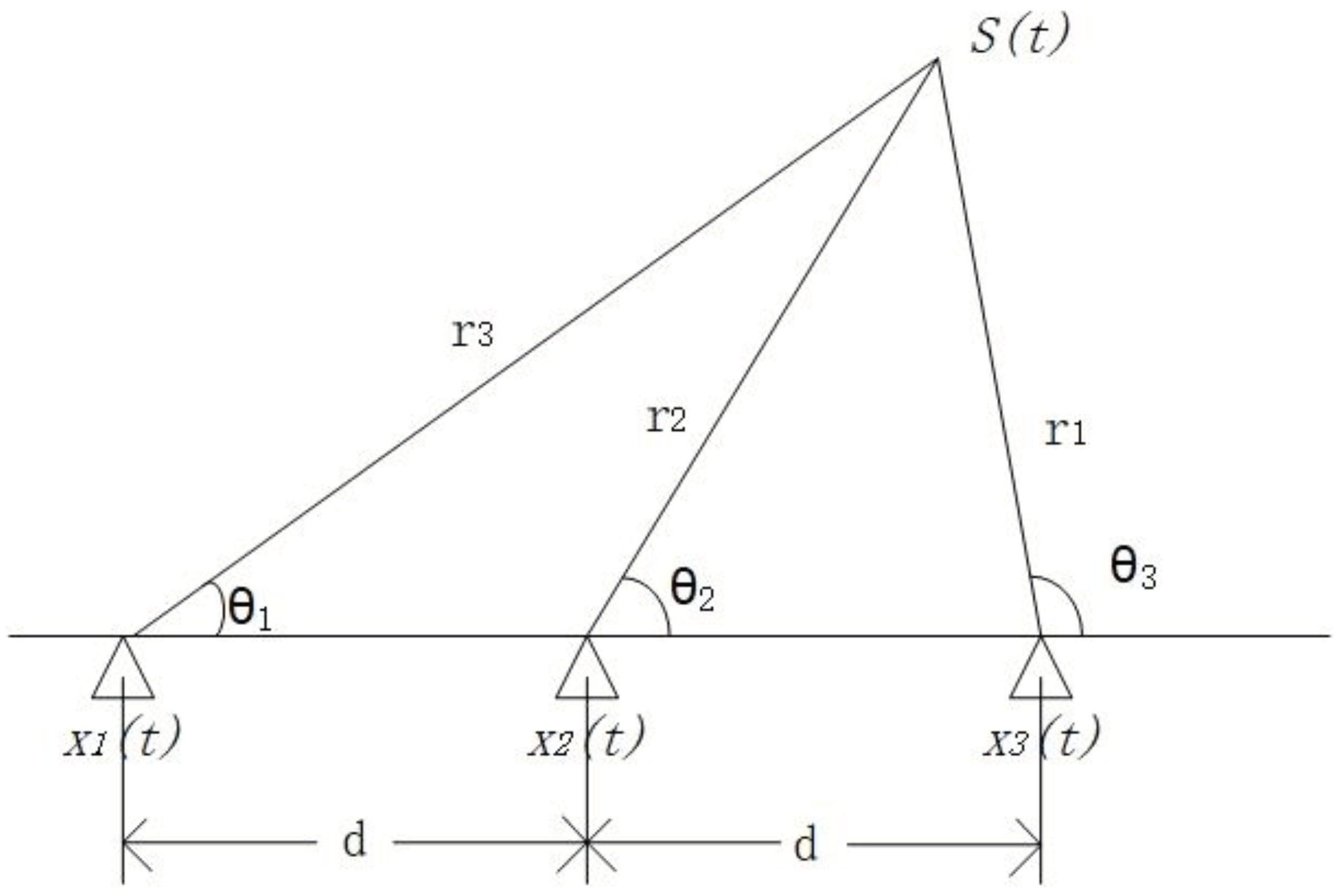
The near-field model requires three and more numbers of microphones for localisation, using a 3-microphone uniform linear microphone array as an example. The first microphone is chosen as the reference microphone, then and denote the time delay between the acoustic signal arriving at the first microphone and the second microphone and the third microphone , respectively, then the time delay and can be expressed as:
Note: —is the distance from the point source to the i microphone, —is the velocity of propagation of the acoustic signal in air (generally taken as an approximation of 340 m/s)
2.2. Ternary Discrete Distributed Microphone Arrays
The acoustic signals received by microphone arrays based on the near-field model are spherical waves with high correlation between the signals. By increasing the aperture of the array, the reception range of the spherical wave can be enlarged, i.e., the practical application area of the microphone array can be increased. Therefore, a discrete distributed microphone array is selected, as shown in Figure 1.2.
Figure 1.2.
Ternary discrete distributed microphone arrays.
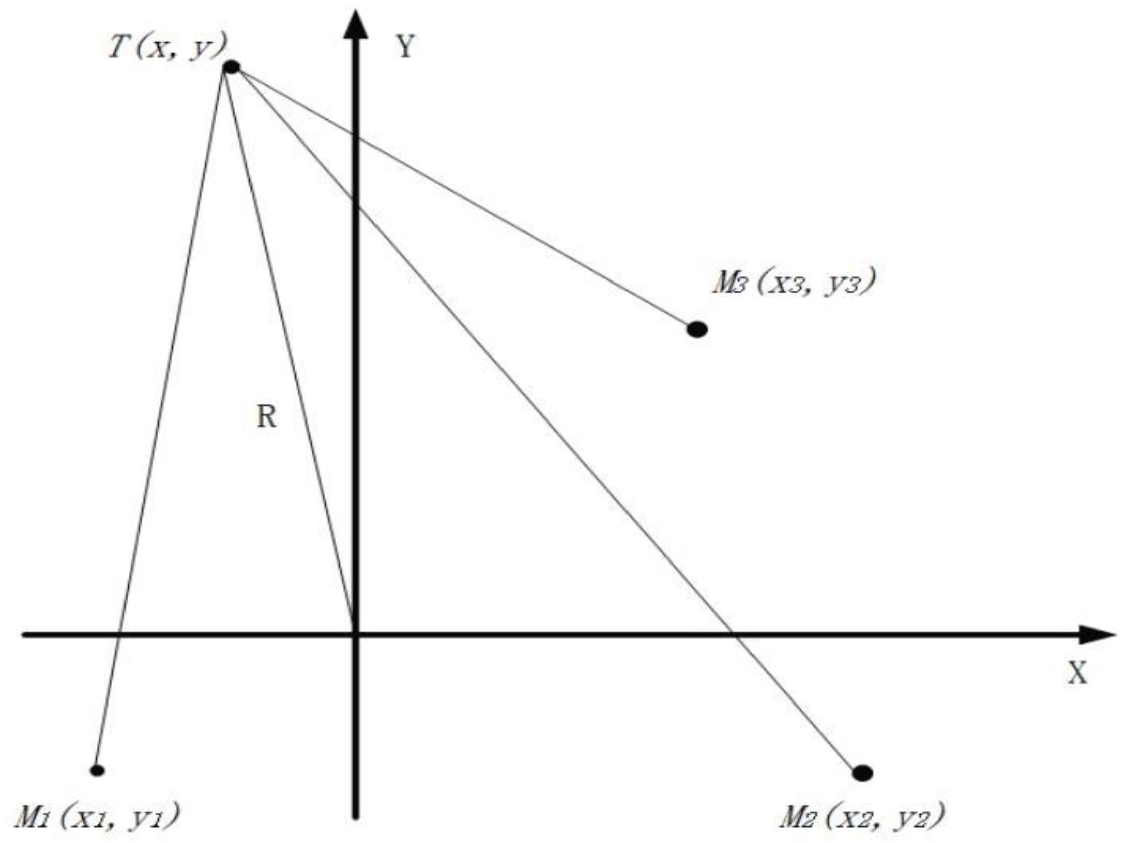
In the coordinate system , the position of the three microphones are , and . The array of three microphones can be flexibly arranged, let be the true position of the point source, the distance from to the origin of the coordinate system is the drop-off distance , the distance to each microphone is , and the time at which the signal arrives at the reference microphone is . According to the geometrical relationship can be obtained:
Substituting into equation (3) and transforms into a polar equation:
The simplification can be obtained:
The hyperbolic intersection system of equations for ternary discrete distributed microphone array can be obtained from equation (4), and the position information of the target can be obtained by solving the hyperbolic system of equations, due to the fact that this hyperbolic system of equations is a nonlinear system of equations, which is often accompanied by more than one solution or virtual solution, etc., which makes it difficult to solve, and can be transformed into a system of linear equations and then solved first.
In the actual experiment, the array parameters (the real position of each sensor) are pre-determined according to the field conditions, and the correlation processing of the signals is carried out to obtain the time delay between the microphones, so that the location of the drop point can be determined.
3. Time Delay Analysis of Sound Source Signals
3.1. Frequency Window Robust Empirical Modal Decomposition Method
3.1.1. Empirical Modal Decomposition (EMD)
The empirical modal decomposition method (EMD) is a method of signal decomposition based on the time scale characteristics of the data itself without any predefined basis functions. Theoretically, it can achieve time resolution and frequency resolution in any dimension, providing a new method for analysing and guiding smooth and nonlinear signals[9,10]. Due to its own characteristics, EMD makes the method theoretically applicable to the decomposition of any type of signals, and it has very obvious advantages and high signal-to-noise ratios in dealing with non-smooth and nonlinear data.
The traditional EMD decomposition steps can be categorised as follows [13]:
- (1)
- Find all extreme points of the original signal.
- (2)
- Fitting the upper and lower envelopes by using cubic spline curves.
- (3)
- Find the mean of the upper and lower envelopes, and draw the mean envelope .
- (4)
- The original signal minus the mean envelope to get the middle signal .
During the generation of intermediate signals, a conditional judgement on is required:
1、In the interval, the number of extreme points and the number of points past zero must be equal or differ by at most one.
2、At any time, the average value of the upper envelope formed by the local maxima and the lower envelope formed by the local minima is zero.
When the above conditions are met an IMF component can be generated, the algorithm updates the original signal and repeats the process.
Note: is the first-order IMF component and denotes the updated signal.
3.1.2. Robust Empirical Modal Decomposition with Adaptive Frequency Windows
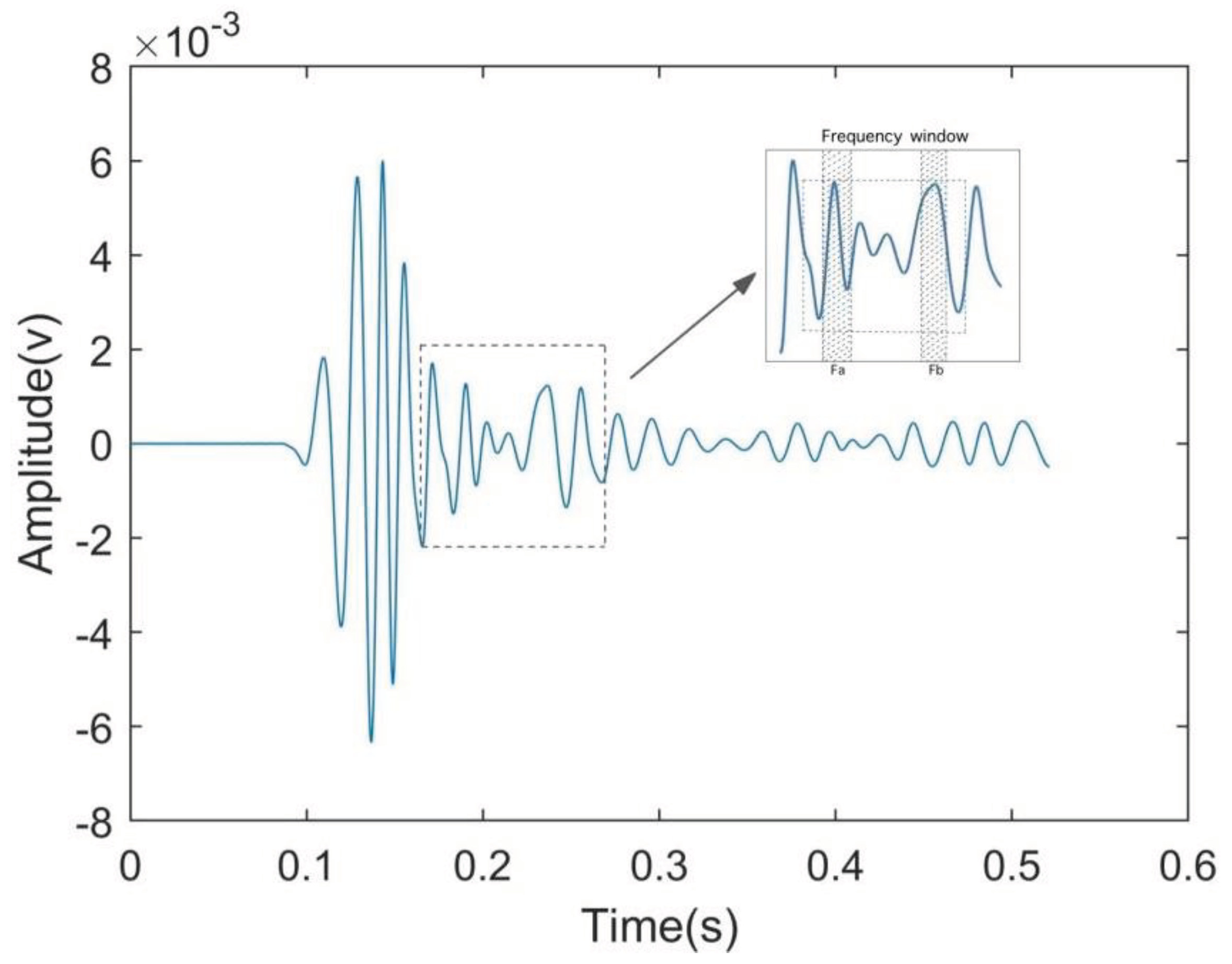
This paper proposes the use of adaptive frequency window in the signal spectrum locking and extraction, in order to solve the original signal segmentation in the face of the problem of missing spectral boundaries, the process is shown in Figure 2.1, the frequency window shown in the Figure as , where for the window before and after the cut-off band of the centre frequency, the shaded portion of the segmentation of the width of the segmentation of the excessive region of . Frequency window by comparing the frequency threshold in the window, in this range of free sliding, until the similarity exceeds the index can be locked position, the frequency window of the bandwidth of the size of the variable range.
Figure 2.1.
Adaptive Frequency Window.
As the traditional EMD algorithm adopts cubic spline interpolation in the decomposition, the algorithm has endpoint effects when decomposing the IMF, which leads to signal distortion, and there is a large error in the decomposition of the obtained IMF time axis, and the principle of the algorithm leads to modal aliasing phenomenon in the decomposed IMF, and when the signal-to-noise ratio of the original signal is lower, the signal-to-noise ratio of the decomposed IMF is also lower, and the effect becomes larger in further decomposition. When the signal-to-noise ratio of the original signal is low, the signal-to-noise ratio of the decomposed IMF is also low, and the effect becomes bigger in further decomposition. Since the UAV flight sound is still mixed with noise in different frequency intervals during the process of being received by the sensors, it is necessary to improve the traditional EMD algorithm to adapt to the scenarios applied in this paper.
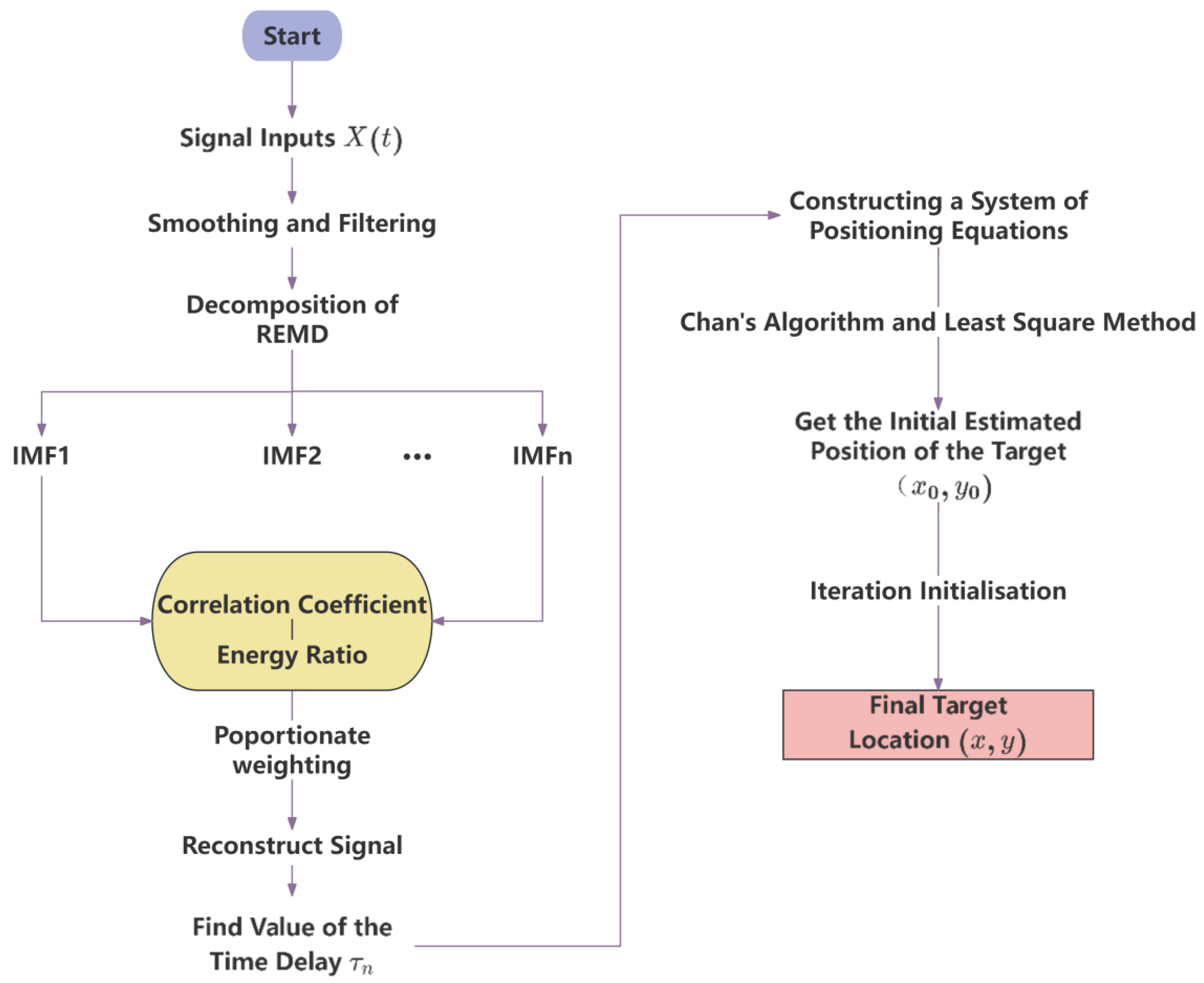
Aiming at the phenomena existing in the traditional EMD, combined with the application requirements of sound source localisation, this paper adopts the improved empirical modal decomposition algorithm [11], i.e., Robust Empirical Modal Decomposition (REMD), the main idea of REMD is to reduce the influence of noise in the process of signal decomposition and to improve the stability and reliability of the decomposition through the introduction of some robustness criterion or regularization term. By adjusting the regularisation parameter or robustness criteria in the algorithm, the influence of noise can be reduced while retaining the signal characteristics. When the adaptive frequency window locks and splits the original signal, the high and low frequency signals in the split signal are decomposed by weights and the decomposed IMF components are reconstructed, so as to obtain the reconstructed signal with high signal-to-noise ratio, and the specific implementation process is shown in Figure 2.2.
A REMD decomposition of the segmented signal is performed and the decomposition yields n IMF components;
Note: is the improved robust intrinsic modal function and is the residual term.
- (1)
-
Filter the components with higher signal-to-noise ratio according to the following reconstruction criterion [15].
- 1.
-
Correlation coefficientCorrelation coefficient is a statistical indicator of the close connection between the response variables, in this paper Pearson's correlation coefficient, which is commonly used in statistics, is used. The degree of correlation between X and Y is described by the value in the interval [-1, 1], the larger the value of the coefficient, the higher the correlation, and vice versa. After performing the REMD decomposition, the algorithm automatically calculates the correlation coefficients between the IMF components and the segmented signals as a way to differentiate the useful components and retain them. Let two samples be X and Y. The following equation represents the Pearson correlation coefficient of two continuous variables , which is equal to the product of the covariance between them divided by their respective standard deviations . Variables close to 0 are made uncorrelated and those close to 1 or -1 are said to be strongly correlated.
- 2.
- Amplitude ratio
The mathematical expression for the energy ratio coefficient is
Where, is the total energy of the IMF component; is the energy of different IMFs; is the energy ratio coefficient.
- (2)
- According to the proportional weighting method, take the maximum correlation coefficient as IMFmax(n) and the minimum correlation coefficient as IMFmin(n), subtract the two components and compute the average value, add the value to the segmented signal and reconstruct it to obtain a signal with high signal-to-noise ratio.
- (3)
- Analyse the trigger time values in the reconstructed signal and output the trigger time to which the microphone sensor was subjected.
Figure 2.2.
Positioning Flowchart.
3.2. GWO-Based Adaptive Optimisation
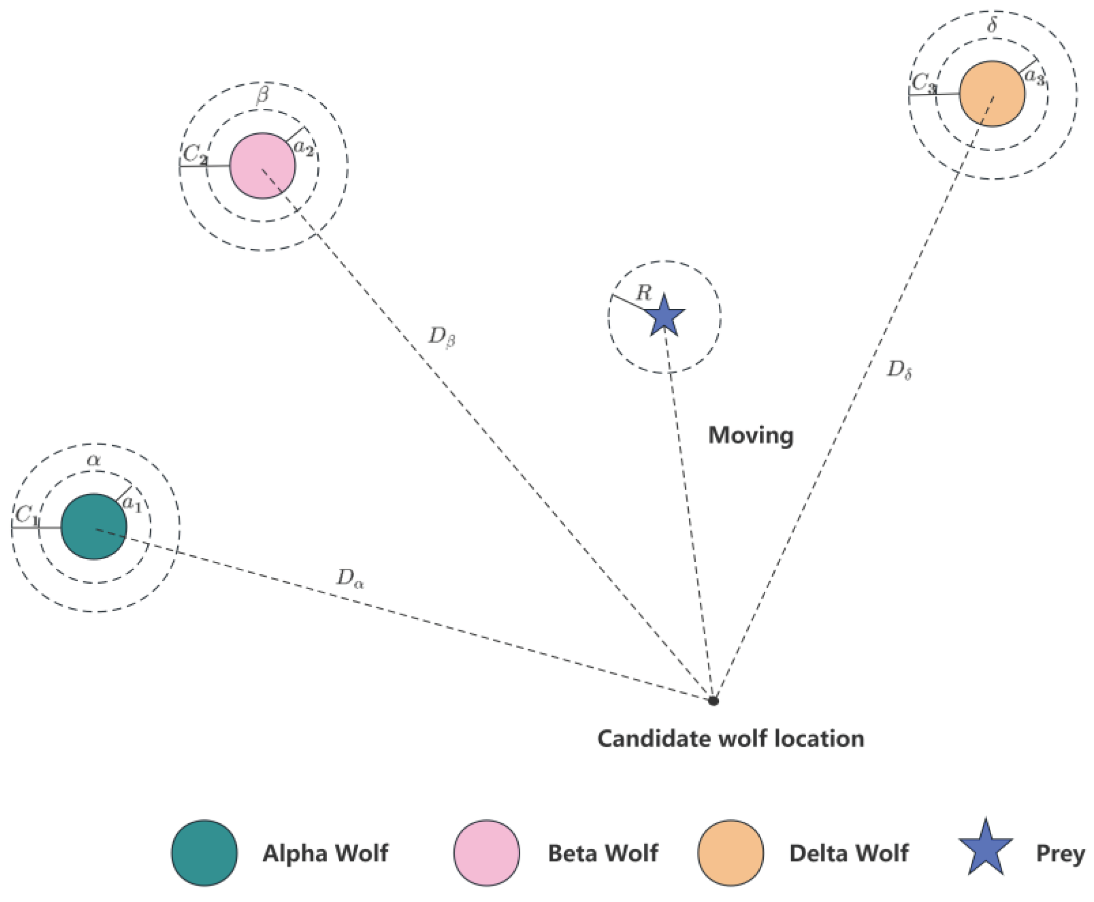
The Grey Wolf Optimization (GWO) algorithm [12] is inspired by the grey wolf packs in nature, and the GWO algorithm simulates the hierarchy and hunting mechanism in the grey wolf packs in nature [14]. The grey wolf optimization algorithm does not require complex parameter tuning, and at the same time, it has a strong global search ability, which can quickly find the optimal solution, and the article seeks the optimal fitness function of the adaptive frequency window with the help of the advantages of this algorithm.
GWO classifies the entire wolf population into Alpha, Beta, Delta, and Omega wolves according to the fitness curve, with wolves decreasing in rank in the following update process:
- (1)
- Calculate the distance between an individual grey wolf and its prey and update the grey wolf's position at all times:Where, is the number of moment iterations; is the distance between the individual grey wolf and the prey; is the position vector of the prey; is the position vector of the individual grey wolf; and is the coefficient vector, which is calculated as:Where, is the random vector in the interval [0,1], is the maximum number of iterations, and is the convergence factor.
- (2)
- Grey wolves are able to identify the location of their prey and surround them. When the grey wolf identifies the location of the target, and guide the pack to encircle the prey under the leadership of . And constantly update their positions, their tracking mathematical model expression is:Where, and denote the distance between and and other individuals, respectively; and represent the current positions of and , respectively; are random vectors and is the current position of the grey wolf. Eqs. (21)-(23) denote the step length and direction of individual in the wolf pack towards e,f and g, respectively, and Eq. (24) denotes the final position of .
The coefficient vector A in Eq. (15) represents a random value in the interval [-a, a], and during the attack process of the wolf pack, the value of a is gradually reduced, while the range of fluctuation of is also reduced. When , the wolf pack approaches and captures the prey, i.e., the optimal solution is obtained, and when , the grey wolf separates from the prey and searches for a more suitable target. In this paper, the noise ratio in the frequency domain is used as the fitness function of the frequency window, and the GWO is used to adaptively determine the window position.
Figure 2.3.
Schematic diagram of the GWO adaptive algorithm.
4. Improved Sound Source Localisation Algorithms
4.1. TDOA Algorithm
The TDOA algorithm works by measuring the time differences between signals received by different receivers and using these time differences to calculate the position of the transmitting source.Specifically, it is assumed that there are three or more receivers with known relative positions to each other, and that when the source transmits a signal, each receiver records the time at which the signal is received.Since the velocity of signal propagation is known, this time difference and velocity information can be used to construct a system of localisation hyperbolic equations to calculate the position of the signal source. However, this hyperbolic system of equations tends to be nonlinear and the obtained solution is often imaginary or no solution, which needs to be solved by transforming the nonlinear system of equations into a linear system of equations.The mainstream methods are Fang algorithm,Chan algorithm and Taylor algorithm.
In this paper, Chan's algorithm and Taylor's algorithm are selected and five different sizes of Gaussian white noise are selected for simulation. Figure 3.1 (a), (b) and (c) represent the Chan algorithm measurement noise standard deviation, Taylor algorithm measurement noise standard deviation, Chan and Taylor algorithm measurement noise standard deviation, respectively.
Figure 3.1.
Different algorithms for measuring standard deviation.
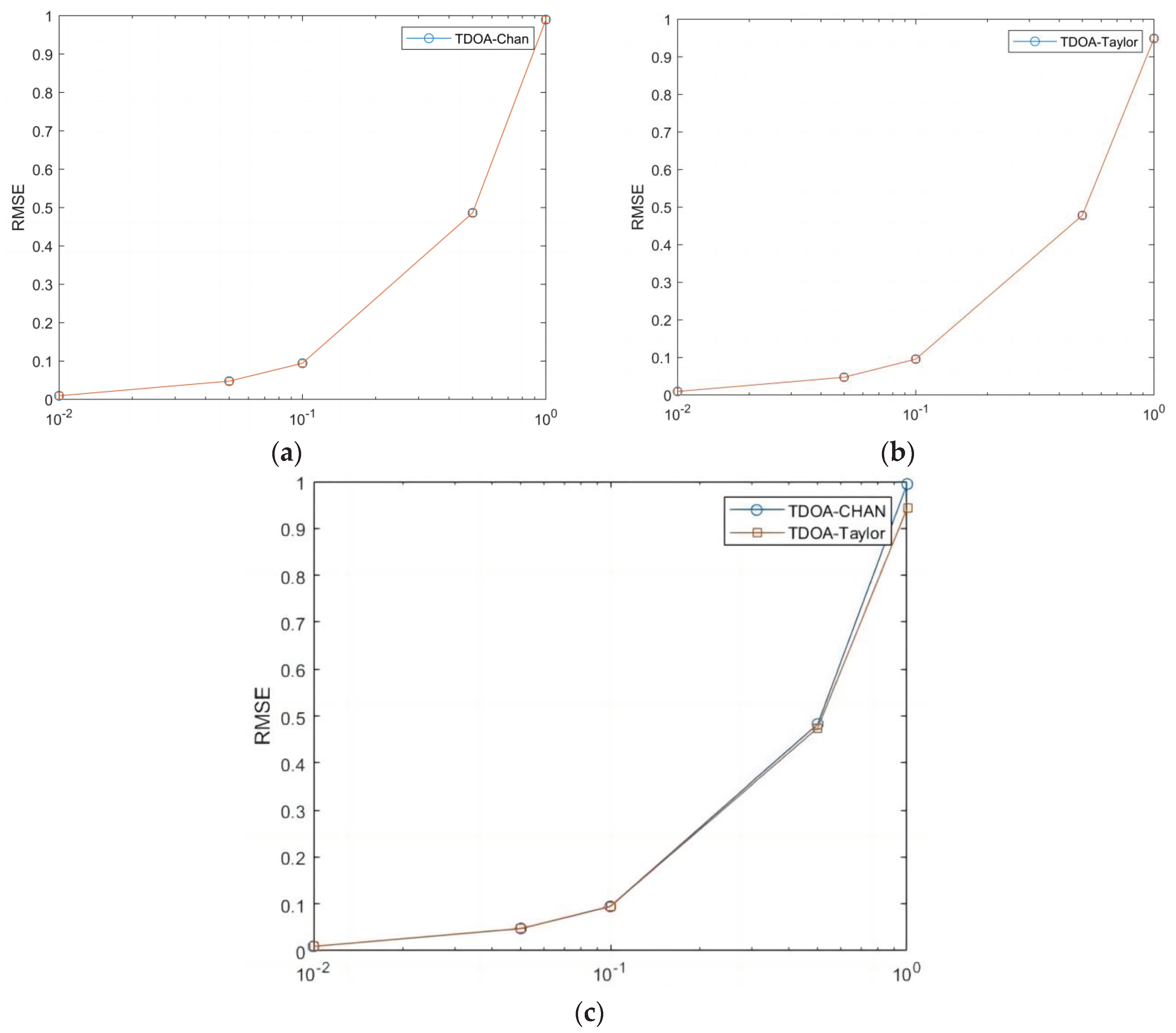
The simulation results in Figure 3.1(c) show that the RMSE (Root Mean Square Error) of Chan's algorithm and Taylor's algorithm are basically the same when the noise is small; as the noise of the measurements gets bigger and bigger, Taylor's algorithm's RMSE is obviously better than Chan's algorithm.
4.2. Improving the Chan-Taylor Localisation Algorithm
As Chan algorithm [4] can make full use of the information of TDOA measurement value of each base station, it can effectively reduce the negative impact of the large measurement error of individual base stations on the positioning, and Taylor algorithm obtains higher positioning accuracy when the initial position selection accuracy is higher. Therefore, in this paper, Chan algorithm and Taylor algorithm will be fused to locate the position of experimental micro UAV, and five different sizes of Gaussian white noise are selected for simulation.
The principle of Chan-Taylor joint positioning algorithm is to use the Chan algorithm to estimate the initial coordinates of the target after the Chan algorithm, and then carry out Taylor iterative calculations to constantly update the position label obtained by the method that more closely resembles the true position. In this paper, Chan-Taylor algorithm [7,8] is selected and combined with the weighted least squares method for solving.
The specific algorithmic process is as follows:
- (1)
- Initial estimation of the target's true position using Chan's algorithm. The position of microphone is known to be . Assuming that the true position of the target is , it can be known:
Let , according to equation (25) then we have:
According to equation (26) then we have:
Substitute equation (27) into equation (28) and let ;
This step eliminates the squared terms of the unknowns and preserves a series of linear equations which, when , gives the following expression:
The solution can be obtained:
Let
Then Eq. (31), Eq. (32) can be simplified to the following calculation equation:
Substituting Eq. (33) into Eq. (29) and such that
A quadratic equation about can be obtained:
Solve the equation for the two roots available, omit the invalid solutions, and substitute the valid solutions back into Eq. (12) to obtain the estimated coordinates of the location point .
- (2)
- Substitute the estimated coordinates obtained by Chan's algorithm as the initial values of Taylor's series expansion method.Let the true coordinate value of the target be :
Then the Taylor series expansion of the function at is as follows:
Substituting equations (25) and (26) into equation (36) gives:
By performing a Taylor expansion of at and neglecting components above second order, we have:
Translated into matrix form, there:
Notes: is the error vector.
Let:
- (3)
- Solve the weighted least squares solution of the above equation [6]:where is the covariance matrix of the noise measurements, and in the next iteration of the computation, let . The above computation process is repeated until the error stops when it meets the set threshold, i.e. .
The obtained at this point is the final positioning coordinate of the target that is infinitely close to the true value after iterative calculation.
5. Simulation Verification and Analysis
In this section, the performance and robustness of the proposed localisation algorithm is tested, and 4.1 and 4.2 are experimentally verified by simulated and real signals, respectively, to demonstrate the accuracy and feasibility of the sound source localisation algorithm proposed in this paper in the use of UAV localisation.
5.1. Algorithm Stability Validation
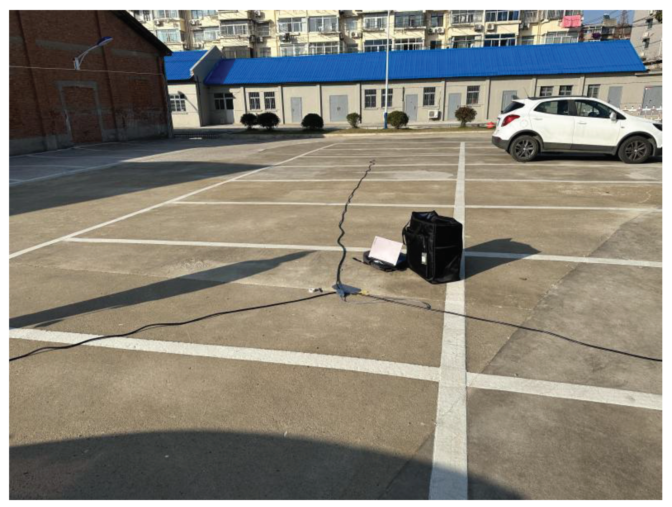
According to the analysis of the characteristics of UAV flight, the signal generated by the rotating blades when the UAV accelerates can be regarded as a short-time impact signal, which is characterised by the peak value of the signal after a period of time, and then slowly diminishes with time. Due to the complex environment around the experiment, this will cause the UAV flight signal to be interfered by some kind of high-frequency vibration signal in the air and land, so the received signal will have a high-frequency vibration signal with higher energy and a random white noise signal with lower amplitude. Therefore, we created such a similar environment in the laboratory, the hardware equipment selected DAQ122 acquisition card and MEMS digital microphone, the signal collected through the host computer is shown in Figure. Using this analogue signal to compare with the algorithm proposed in this paper with EMD algorithm respectively, this paper uses Matlab 2022b version for simulation, the simulation results are shown in Figure.
Figure 4.1.
Site Layout.
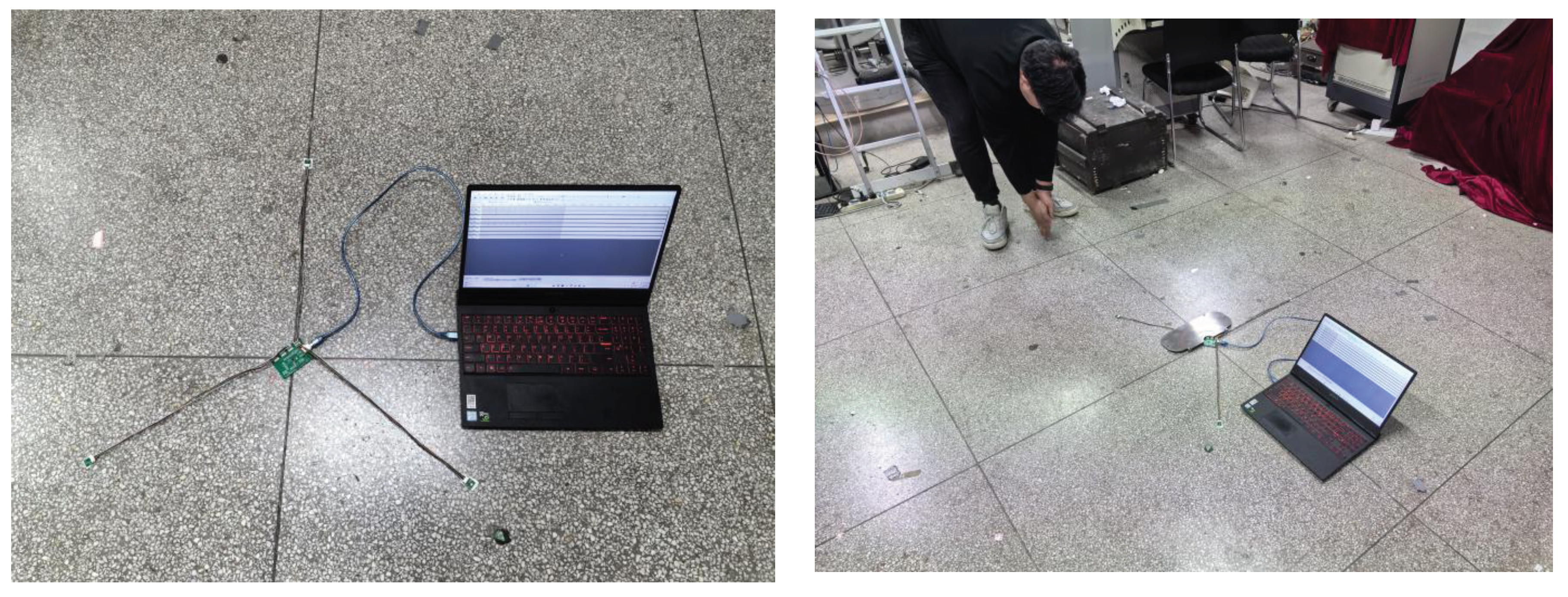
Figure 4.2.
Simulated acoustic signal time-domain diagram.
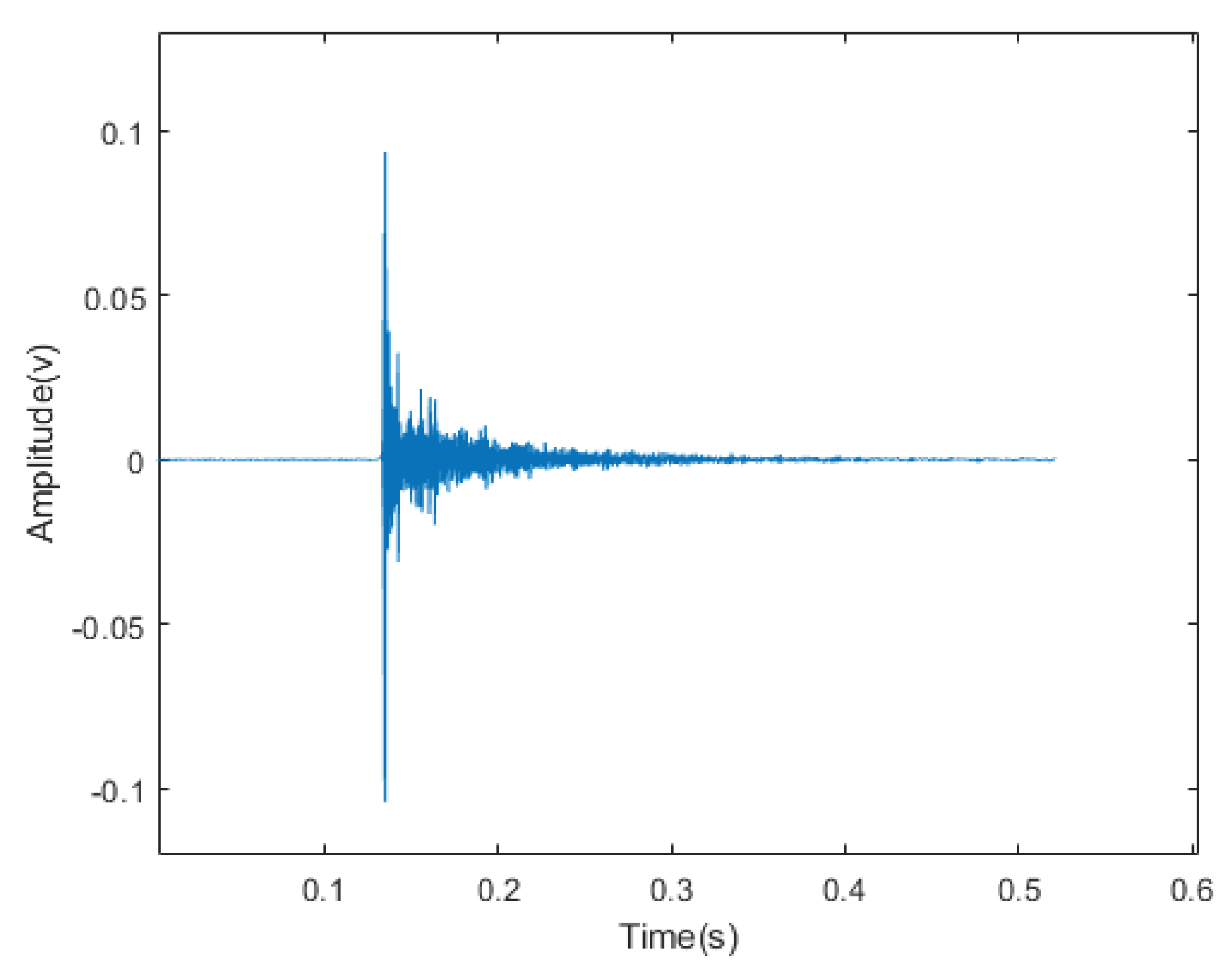
Figure 4.3.
IMF decomposition of the EMD algorithm for simulating acoustic signals.
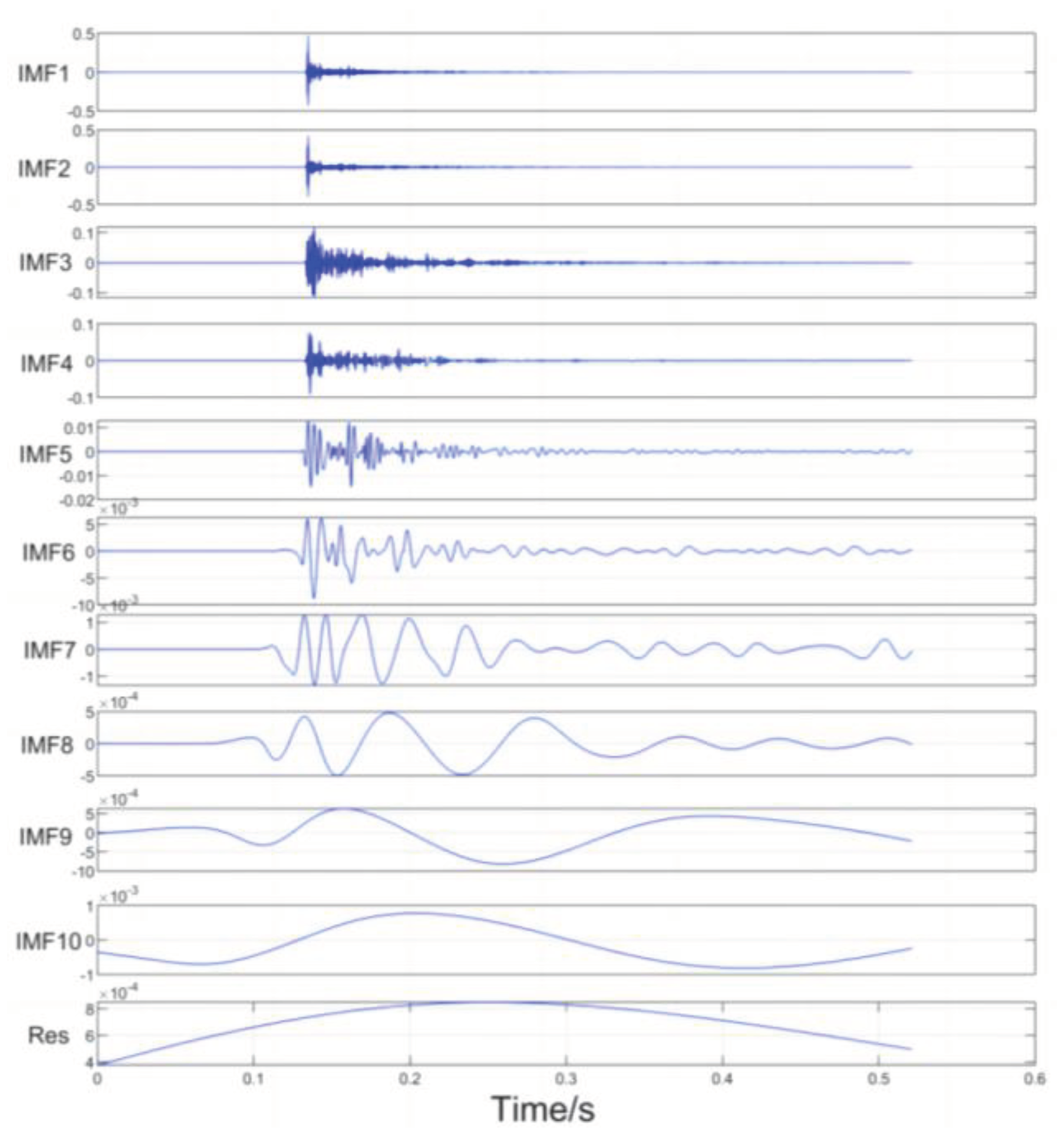
Figure 4.4.
IMF decomposition of the REMD algorithm for simulating acoustic signals.
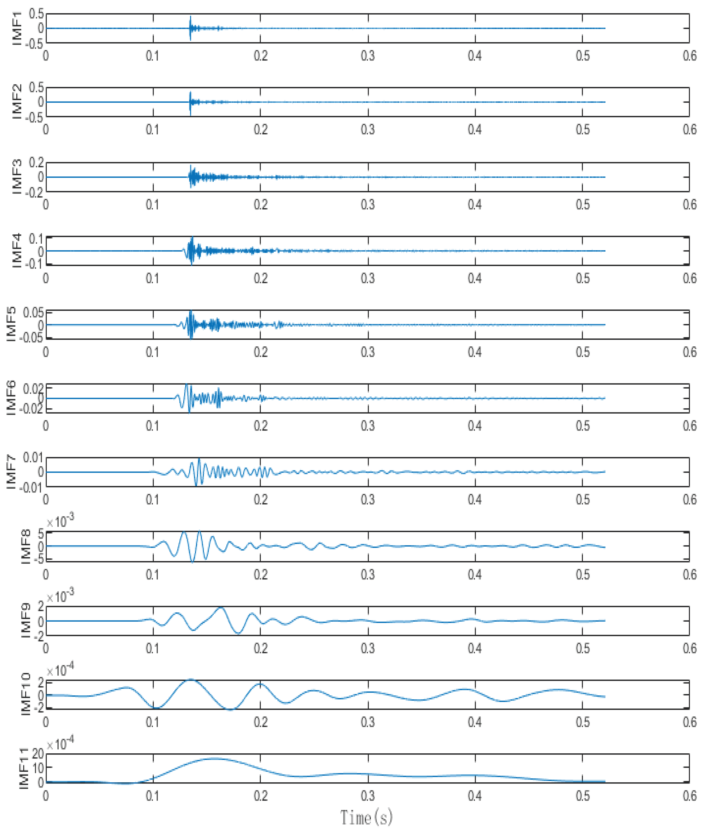
From the above Figure it can be seen that the IMF decomposition obtained after the REMD decomposition of the collected signal shows that the orthogonality between the IMFs is greatly improved, which makes the decomposed IMFs more independent, and at the same time, after the improvement of the robustness, each IMF is more accurately capture the local features of the signal, which greatly improves the localisation performance of the later signal reconstruction with the adaptive sliding window.
5.2. Real Signal Simulation Experiment
In the test area, in order to prevent the influence of human manipulation on the UAV flight position, the pre-collected acoustic signals of the UAV accelerating upwards were used to simulate the UAV flight and to carry out the system validation test. In the experiment, the actual position of the sensor is pre-set and the position coordinates are further corrected by differential GPS; the UAV flight signals are collected by the acoustic sensors after playback, and in this experiment, the recorded acoustic signals of the UAV flights are played back using an amplifier at a selected point, and the signal is collected and processed by the microphone array in the test site, and the time-delay value is obtained to perform the localisation using the TDOA algorithm, and the system records the results of each solution and compares the positioning results with the pre-set real target point to evaluate the positioning accuracy and system robustness.
Figure 4.5.
Map of sensor positions during the test.
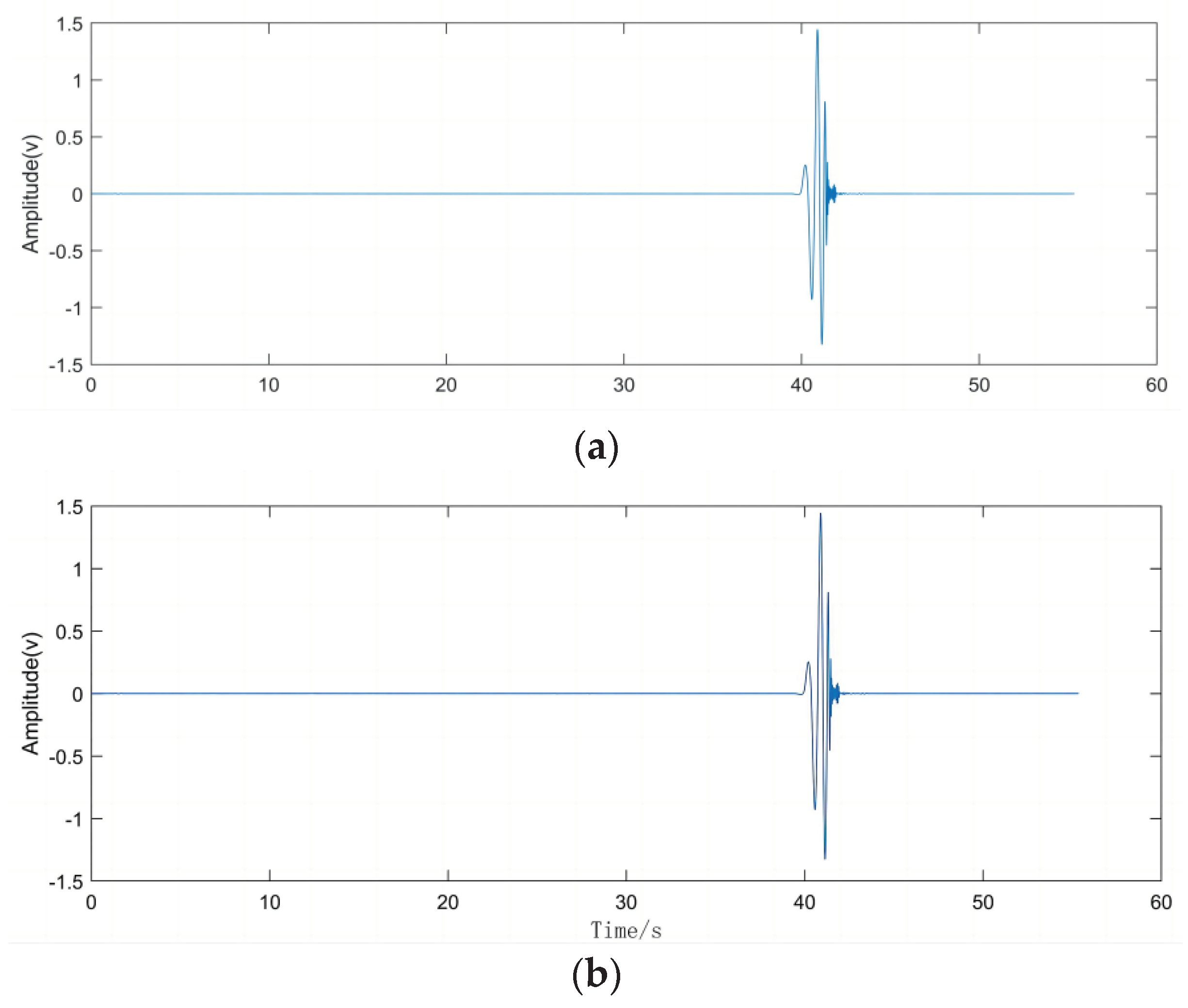
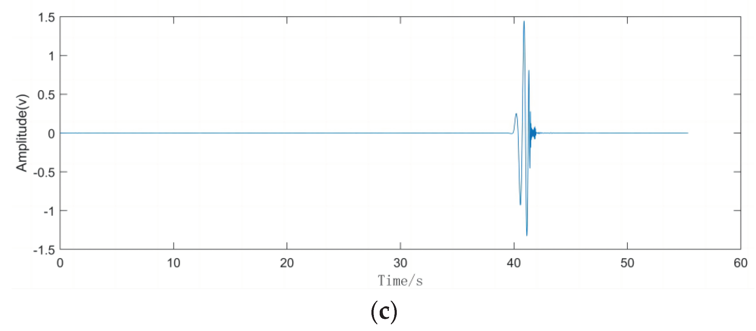
A total of ten valid tests were conducted in the experiment. Figure 4.6 gives a schematic diagram of the target locations and sensor locations corresponding to the ten tests, and the same section of acoustic signals from the UAV flights was used at each playback point with uniform signal decibels. Figure 4.7 shows the pre-collected drone flight acoustic signals collected by the three microphone sensors in the first experiment. It is known from the pre-test that the signals collected by the sensors in the test are basically the same as the pre-collected drone flight signals, and therefore can be used as the simulation signals for the test, and at the same time there is a slight ambient noise around the experiments, such as the wind, the people walking around, and the vehicles driving.Table 1 for the system to resolve the signal collected by the trigger moment record table, Table 2 for the ten tests of the real landing point and the system positioning estimate landing point , and calculate the positioning error .
Figure 4.6.
Schematic diagram of the corresponding target points and sensor positions in the test.
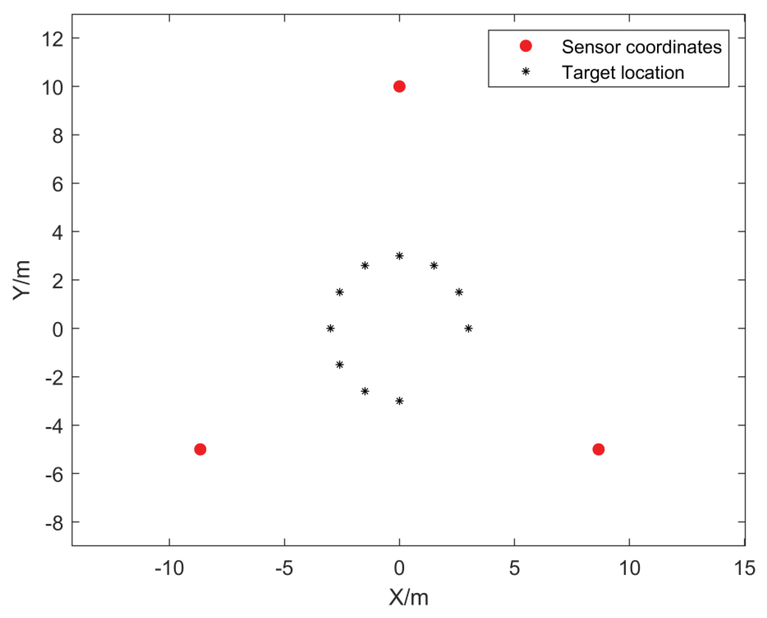
Figure 4.7.
Waveforms of the signals collected by the three array microphones.
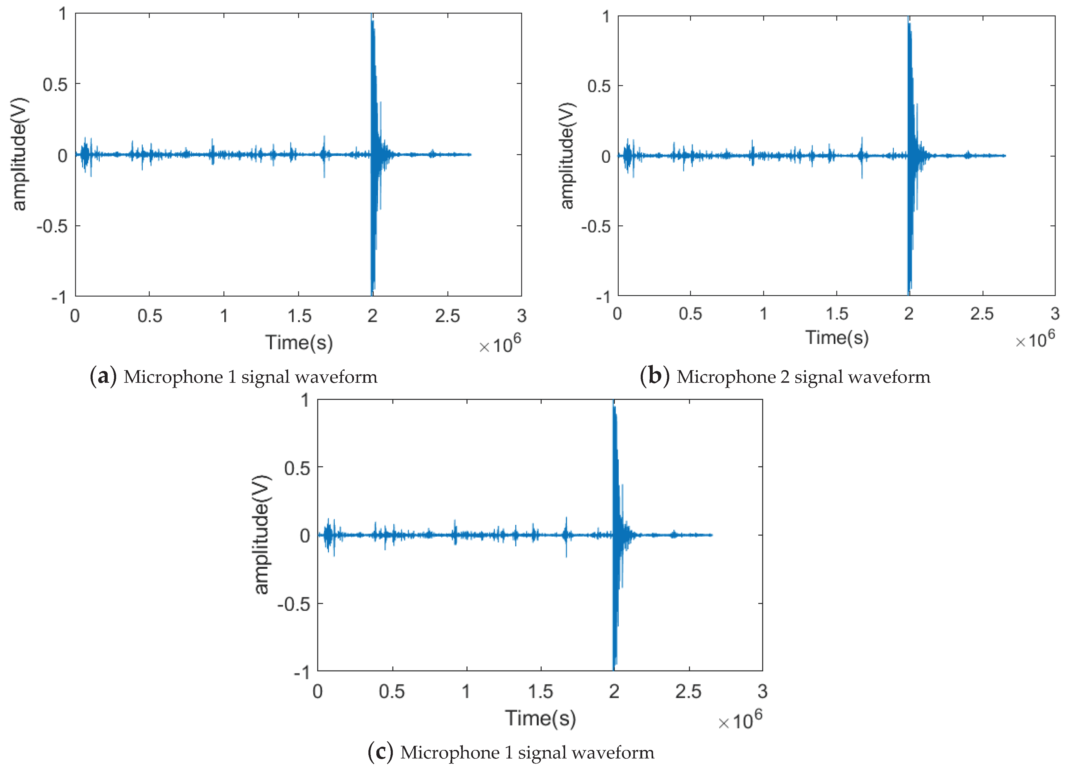
Figure 4.8.
REMD decomposition of the signals collected by the three array microphones.
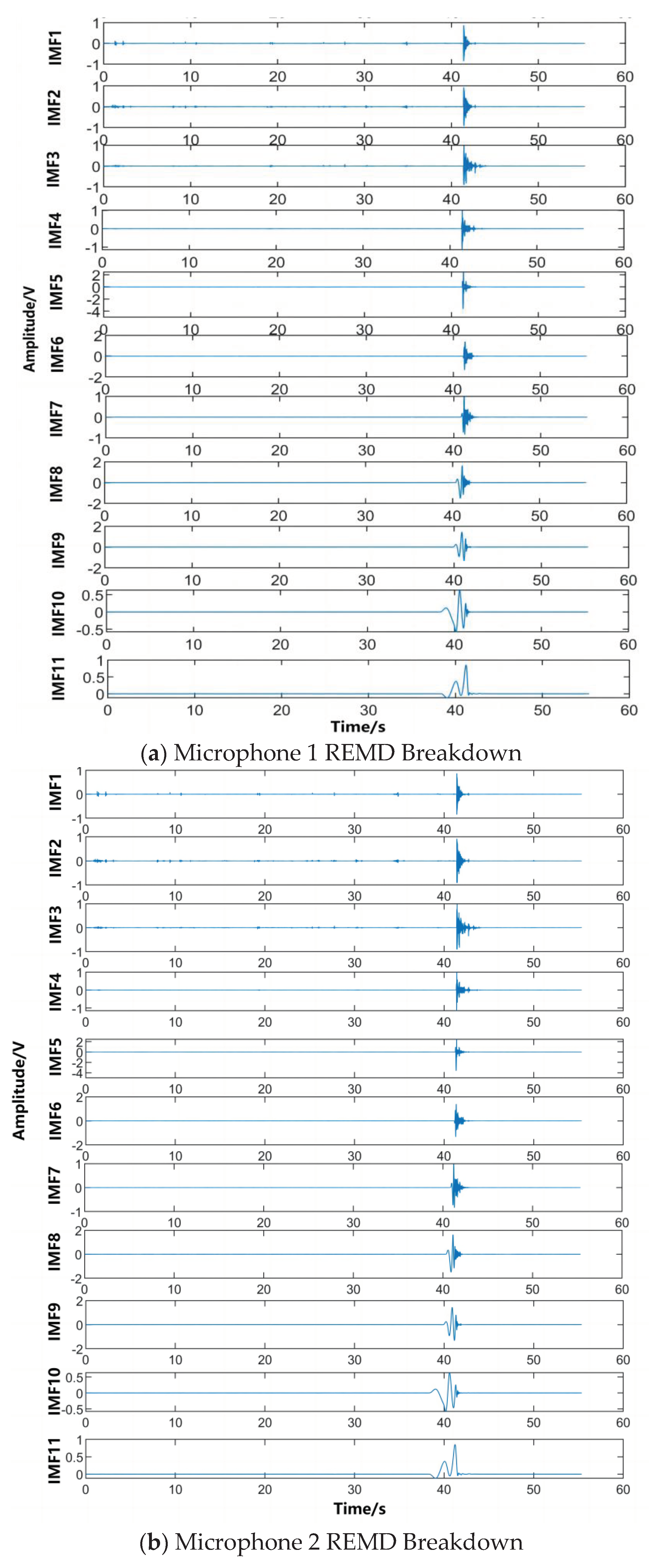
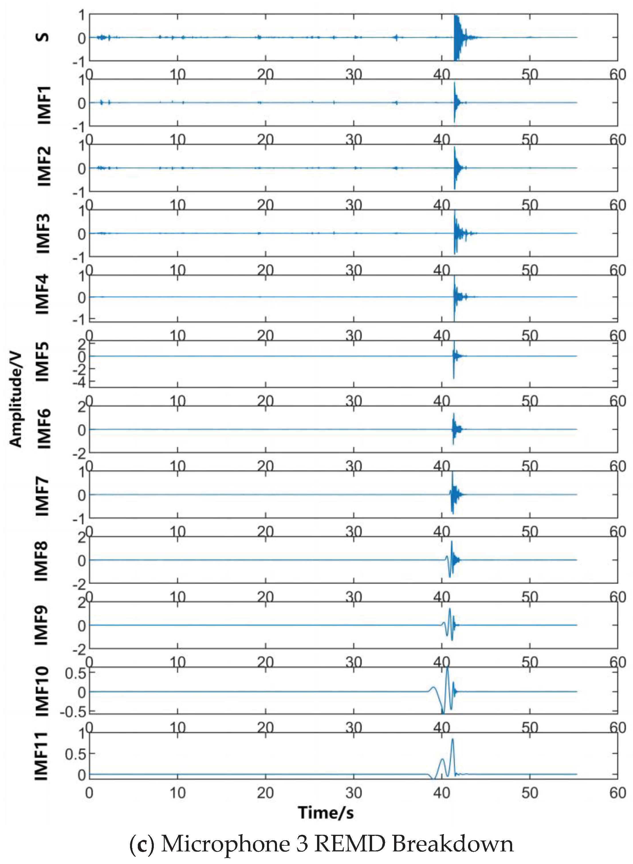
The signal spectrogram is obtained after the FFT transform, and the corresponding frequency matching and extraction is carried out by a translational frequency window with variable bandwidth, and the signal reconstructed by the screening criterion is shown in Figure 4.10, and by parsing the data and using the algorithm to calculate the difference between the reception moments of the different sensors, the moments of the triggering signals in the extracted IMF components are derived and recorded, and according to this process, the time delays obtained from the nine remaining experiments are The results are recorded in Table 1, while the estimated position coordinates are compared with the actual measured coordinates using the positioning algorithm in this paper, and the error values are calculated and recorded in Table 2;
Figure 4.9.
spectrogram.
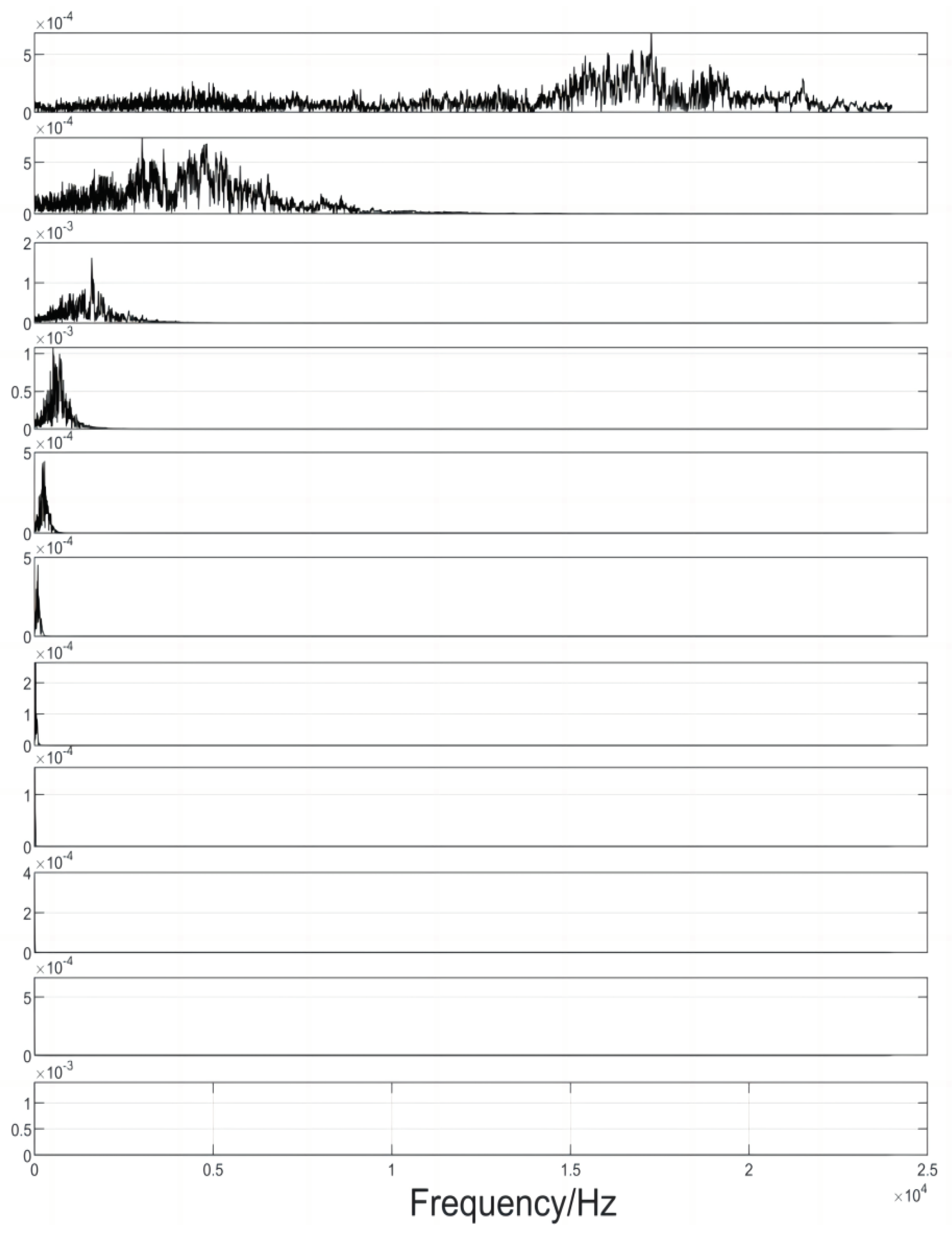
Figure 4.10.
Reconstructing the IMF Trigger Signal Moment Chart.
As can be seen from Table 1 and Table 2, under the same experimental environment, after the resolution of the sound source localisation algorithm with improved empirical modal decomposition under the adaptive frequency window, the estimation errors of the localisation within the range of the collectable signals are all below 5%, which indicates that under the algorithm of this paper, the time delay estimation value resolved by the decomposed signals greatly improves the success rate of the location estimation, and the algorithm, whether it is for near-field or far-field, has a good performance under the presence of random noise, but of course, in the experiments it was found that the localisation accuracy of some locations is still not high enough, and the subsequent algorithms still need to be compensated accordingly for the special values.
6. Conclusions
This paper constructs a UAV detection sound source positioning system based on the EMD empirical modal decomposition algorithm, comparing the traditional GCC (generalised cross-correlation) delay estimation method, in the presence of noise aliasing, the separation of the signals of different frequency bands of the high and low and re-combination, and through the frequency domain analysis of the UAV flight signals before the test, it can be decomposed effectively to get the complete signal of the UAV flight signals from it, and improves the The accuracy of time delay estimation is improved. This also improves the Chan-Taylor algorithm's shortcoming of rapid performance degradation when the accuracy of delay estimation is insufficient. At the same time, the distributed sensor array is freely arranged to expand the positioning area and flexibility.
In this paper, we have not yet tested the real UAV flights in the actual test site, and this test condition is carried out in a high signal-to-noise ratio environment, how to further improve the performance of the EMD empirical mode decomposition algorithm in the presence of noise aliasing similar to that of the UAV flight signals in the frequency domain has become the next step of the research goal.
Acknowledgments
This work was sponsored by Nanjing University of Science and Technology.
References
- Yang, F.; Song, R.Z. A Review of Sound Source Localization Research in Three Dimensional Space. In Proceedings of the IEEE 12th Data Driven Control and Learning Systems Conference (DDCLS), Xiangtan, China, 12–14 May 2023. [Google Scholar]
- Cho, K.; Nishiura, T.; Yamashita, Y.; et al. A Study on Multiple Sound Source Localization with a Distributed Microphone System. In Proceedings of the 10th INTERSPEECH 2009 Conference, Brighton, England, 6–10 September 2009. [Google Scholar]
- He, Q.; Han, K.; Feng, J.; et al. A Sound Source Localization Method for Microphone Array with Arbitrary ConFigureuration. J Xi'an Jiaotong Univ (China) 2020, 54, 186–192. [Google Scholar]
- Yan, X.; Zhang, Z.; Wang, H. Application of Chan algorithm in marine sound source localization. Tech Acoust (China) 2021, 550–555. [Google Scholar]
- Bob, F.I. Embedded Solution for Universal Acoustic Source Distance Localization Using Three Microphones. In Proceedings of the 10th International Symposium on Electronics and Telecommunications (ISETC), Timisoara, Romania, 15–16 November 2012. [Google Scholar]
- Wang, Z.; Yu, H.; Hu, Y. Improved chan algorithm based on maximum likelihood criterion. Computer Applications and Software 2014, 31, 240–243. [Google Scholar]
- Zhou, R.H.; Sun, H.M.; Li, H.; et al. Time-difference-of-arrival Location Method of UAV Swarms Based on Chan-Taylor. In Proceedings of the 3rd International Conference on Unmanned Systems (ICUS), Harbin, China, 27–28 November 2020. [Google Scholar]
- Wang, P.; Zhang, N. A Cooperative Location Method Based on Chan and Taylor Algorithms. In Proceedings of the International Conference on Information Technology for Manufacturing Systems, Macao, China, 30–31 January 2010. [Google Scholar]
- Mohguen, W.; Bekka, R. Comparative Study of ECG Signal Denoising by Empirical Mode Decomposition and Thresholding Functions. In Proceedings of the 6th International Conference on Electrical and Electronics Engineering (ICEEE), Istanbul, Turkey, 16–17 April 2019. [Google Scholar]
- Fleureau, J.; Kachenoura, A.; Albera, L.; et al. Multivariate empirical mode decomposition and application to multichannel filtering. Signal Processing 2011, 91, 2783–2792. [Google Scholar] [CrossRef]
- Lv, T. An improved EMD-based method for series fault arc identification. 2023 8th International Conference on Intelligent Computing and Signal Processing (ICSP) 2023, 1582–1588. [Google Scholar]
- Long, W.; Wu, T.B.; Cai, S.H.; et al. A Novel Grey Wolf Optimizer Algorithm With Refraction Learning. Ieee Access 2019, 7, 57805–57819. [Google Scholar] [CrossRef]
- Chen, Z.; Luo, W.; Chang, J.; et al. EMD-based neural network air-coupled ultrasonic oil storage tank level detection. China Test 2021, 47, 9–14. [Google Scholar]
- Mirjalili, S.; Mirjalili, S.M.; Lewis, A. Grey wolf optimizer. Advances in Engineering Software 2014, 69, 46–61. [Google Scholar] [CrossRef]
- Xiaochi LU, A.N.; Shi, X.U.; Yundong SH, A.; Gongmin LI, U.; Jinyu TA, N.G.; Xi ZH AN, G.; Zhuang, L.I. A rolling bearing fault diagnosis method based on GWO-NLM and CEEMDAN. Journal of Aerospace Dynamics 2023, 38, 1185–1197. [Google Scholar] [CrossRef]

Table 1.
Time estimation results after REMD decomposition.
| serial number | Mic(i#) trigger moment/s | Mic2, Mic3 and Mic1 time difference/s | |||
| 1# | 2# | 3# | α1 | α2 | |
| 1 | 1.7123 | 1.7217 | 1.7282 | 0.00941 | 0.01592 |
| 2 | 1.6272 | 1.63073 | 1.64121 | 0.00353 | 0.01401 |
| 3 | 1.7233 | 1.73083 | 1.73851 | 0.00753 | 0.01521 |
| 4 | 1.2341 | 1.24808 | 1.24808 | 0.01398 | 0.01398 |
| 5 | 1.1752 | 0.18972 | 1.181631 | 0.01452 | 0.006431 |
| 6 | 2.3812 | 2.39351 | 2.38131 | 0.01231 | 0.00011 |
| 7 | 1.4251 | 1.43207 | 1.41696 | 0.00697 | -0.00814 |
| 8 | 2.3127 | 2.3128 | 2.29879 | 0.0001 | -0.01391 |
| 9 | 1.4527 | 1.44636 | 1.33037 | -0.00634 | -0.01498 |
| 10 | 1.8162 | 1.80387 | 1.80387 | -0.01233 | -0.01233 |
Table 2.
Test drop monitoring results.
| serial number | true point of impact | the estimated position | |||
| 1 | 3 | 0 | 2.9935 | 0.0098 | 4.48 |
| 2 | 2.598 | 1.5 | 2.61636 | 1.51643 | 2.41 |
| 3 | 1.5 | 2.598 | 1.49853 | 2.61034 | 1.00 |
| 4 | 0 | 3 | 0 | 3.02133 | 2.13 |
| 5 | -1.5 | 2.598 | -1.48913 | 2.62274 | 1.61 |
| 6 | -2.598 | 1.5 | -2.59035 | 1.49564 | 0.88 |
| 7 | -3 | 0 | -3.02718 | 0.00168632 | 2.72 |
| 8 | -2.598 | -1.5 | -2.59451 | -1.49775 | 0.41 |
| 9 | -1.5 | -2.598 | -1.46837 | -2.75018 | 9.77 |
| 10 | 0 | -3 | -0.0001569 | -3.06854 | 4.85 |
Disclaimer/Publisher’s Note: The statements, opinions and data contained in all publications are solely those of the individual author(s) and contributor(s) and not of MDPI and/or the editor(s). MDPI and/or the editor(s) disclaim responsibility for any injury to people or property resulting from any ideas, methods, instructions or products referred to in the content. |
© 2024 by the authors. Licensee MDPI, Basel, Switzerland. This article is an open access article distributed under the terms and conditions of the Creative Commons Attribution (CC BY) license (http://creativecommons.org/licenses/by/4.0/).
Copyright: This open access article is published under a Creative Commons CC BY 4.0 license, which permit the free download, distribution, and reuse, provided that the author and preprint are cited in any reuse.


