Research on Unmanned Vehicle Path Planning Based on Improved A and DWA Fusion Algorithm

1. Introduction

In recent years, with the rapid development of autonomous driving and unmanned vehicles, autonomous navigation technology has become a crucial aspect of vehicle technology. Among the various components of autonomous driving technology, path planning is indispensable, holding significant research and practical value. Path planning can be broadly categorized into global path planning and local path planning.In 1959, Dijkstra proposed the Dijkstra algorithm [1], which employs a greedy approach to determine the start and end points. The algorithm sets the start point as the center and expands outward with equal probability until reaching the endpoint. In 1968, Hart addressed the issue of excessive search in the Dijkstra algorithm and introduced the A* algorithm [2]. A* algorithm sets traversed and untraversed nodes, incorporates a heuristic function, and identifies the path with the minimum weight. Duchoň optimized the A* algorithm based on grid maps [3], addressing imbalances in grid map weights. Zhao Xiao [4] combined the jump point search algorithm with the A* algorithm, filtering jump points for expansion and replacing unnecessary nodes with jump points to reduce computational load.Previous research [5] dynamically computed the robot’s rotation direction and angle, simplifying the path but increasing runtime with low real-time performance [6]. Some studies employed straight-line and circular arc strategies to eliminate the sawtooth effect for smoother paths [7]. Others used differential methods to reduce the number of turning points but involved extensive mathematical computations [8]. Optimization of the A* algorithm’s heuristic function, improvement of key point selection strategies, and reduction of redundant path points were proposed in other studies. Expanding the neighborhood from 8 to 24 neighbors increased path smoothness by leveraging the robot’s ability to move in small angles [9]. However, these improvements did not consider unknown obstacles, lacking certain dynamic obstacle avoidance capabilities.

The mentioned path planning algorithms assume full knowledge of global information, but due to the unpredictability of obstacles and the complexity of different environments, robots are required to navigate autonomously in uncertain situations. In 1997, Fox et al. [10] introduced the Dynamic Window Approach (DWA), considering physical constraints, environmental restrictions, and current speed to effectively solve obstacle avoidance and trajectory curvature problems. Seder et al. [11] combined Focused D* with DWA to address moving obstacle avoidance. Tuvshinjargal D et al. [12] fused obstacle information from Kinect and sonar, improving motion planning accuracy and robustness. Adaptive adjustment of the objective function’s weight based on obstacle density was proposed in one study to correct path safety and smoothness [13]. Another study applied fuzzy control theory, dynamically adjusting three weight coefficients of the evaluation function using three fuzzy controllers to enhance robot adaptability in dynamic environments [14]. A preferred orientation angle range constraint was proposed in another study, utilizing a trajectory evaluation function to determine the optimal trajectory’s corresponding speed [15].

Despite the merits of these algorithms, traditional DWA algorithms are prone to local optima and fail to achieve global optimality. Additionally, for high-speed unmanned vehicles, the lack of timely braking may lead to collisions with obstacles. Therefore, this paper introduces a collision risk evaluation function to enhance obstacle avoidance for unmanned vehicles. Through MATLAB simulation, the improved DWA algorithm is compared with the Dijkstra algorithm and RRT algorithm to ensure its effectiveness. Simultaneously, this paper integrates the DWA algorithm with the A* algorithm to ensure that while using the DWA algorithm to avoid local optima, it can also consider global path planning. A comparison with the separate A* and DWA algorithms shows that the integrated approach yields smoother, more efficient, and shorter paths.

2. Traditional Algorithms and Improvements

2.1. Traditional DWA Algorithm

The DWA algorithm (Dynamic Window Approach) is a commonly used local obstacle avoidance method. This algorithm confines the sampling space for velocity within a dynamically adjustable window. Through optimization based on an evaluation function, it can directly plan the optimal speed for the vehicle. This approach helps avoid potential collisions with obstacles within the speed search space. The algorithm simulates the vehicle’s trajectory over a specified period under these selected speeds.

The DWA algorithm primarily involves three steps: firstly, sampling the vehicle’s velocity based on the environment and the vehicle’s own information; secondly, predicting multiple trajectories based on the sampled velocity information; and finally, selecting the optimal trajectory for path planning according to a predefined evaluation function [16,17].

The DWA algorithm heavily relies on velocity space sampling, with the sampling process being primarily constrained by linear velocity and angular velocity.

$$V_i=\left\{(v,\omega )\right|v\in [v_{min},v_{max}]\cap \omega \in [{\omega }_{min},{\omega }_{max}]\}$$

(1)

In this context, $V_i$represents the velocity space of the unmanned vehicle, $v_{min}$denotes the minimum linear velocity of the vehicle, $v_{max}$represents the maximum linear velocity, ${\omega }_{min}$denotes the minimum angular velocity, and ${\omega }_{max}$signifies the maximum angular velocity of the unmanned vehicle. Additionally, the unmanned vehicle is also influenced by its own motor performance:

$$\begin{array}{c}{V}_d=\left\{(v,\omega )\right|v\in [v_a-\dot{v}·\Delta t,v_a+\dot{v}·\Delta t]\cap \hfill \\ \omega \in [{\omega }_a-\dot{\omega }·\Delta t,{\omega }_a+\dot{\omega }·\Delta t]\}\hfill \end{array}$$

(2)

In this context, $V_d$represents the achievable velocity range of the unmanned vehicle. $v_a$represents the current linear velocity of the unmanned vehicle, ${\omega }_a$represents the current angular velocity, $\dot{v}$denotes the maximum acceleration/deceleration of the linear velocity, $\dot{\omega }$ represents the maximum acceleration/deceleration of the angular velocity, and $\Delta t$is the time interval.

To prevent collisions between the unmanned vehicle and obstacles, it is necessary to decelerate the moving vehicle to zero before any collision with obstacles occurs. Ensuring the safety of the unmanned vehicle is influenced by environmental safety considerations:

$$\begin{array}{c}{V}_m=\left\{(v,\omega )\right|v⩽\sqrt{2·dist(v,\omega )·\dot{v}}\hfill \\ \omega ⩽\sqrt{2·dist(v,\omega )·\dot{\omega }}\}\hfill \end{array}$$

(3)

In this equation, $dist(v,\omega )$represents the distance between the estimated trajectory corresponding to the velocity$(v,\omega )$ and the nearest obstacle.

Figure 1. Trajectory sampling model

Figure 1. Trajectory sampling model

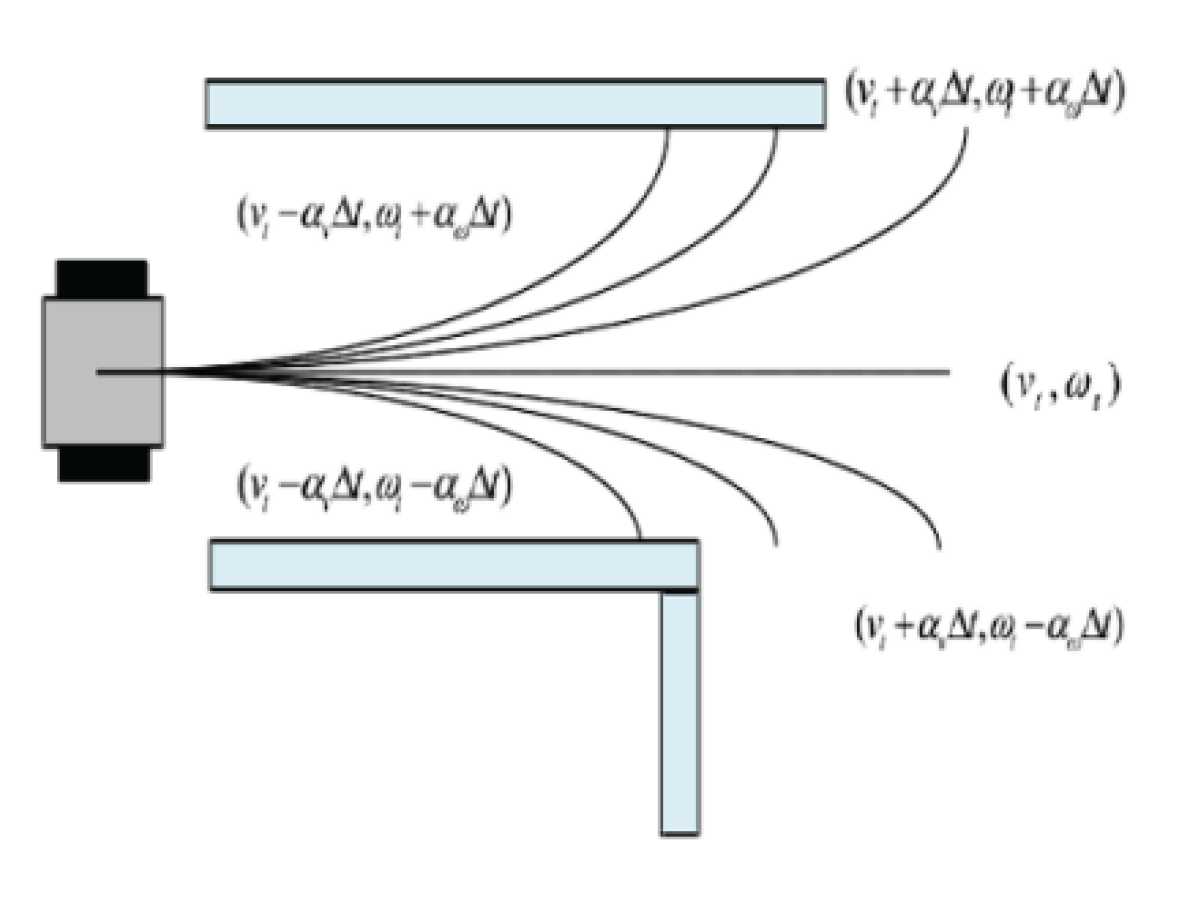
Based on the three constraints mentioned above, the velocity $V_r$of the unmanned vehicle at time $t+1$can be expressed as:

$$V_r=V_i\cap V_d\cap V_m$$

(4)

Building upon the aforementioned three constraints, multiple trajectories are generated using the robot’s kinematic model. These trajectories are then evaluated to identify the optimal one. The guiding principle in designing the evaluation function is to ensure that within the velocity space $V_r$, the robot avoids obstacles and reaches the destination quickly. Based on these requirements, the evaluation function can be formulated as follows:

$$G(v,\omega )=\alpha head(v,\omega )+\beta dist(v,\omega )+\gamma vel(v,\omega )$$

(5)

In this equation, $head(v,\omega )$represents the difference between the heading angle of the robot at the end of the sampled trajectory and the direction angle to the target point. A smaller angle results in a higher score. $dist(v,\omega )$denotes the distance from the end of the sampled trajectory to the nearest obstacle, where a greater distance leads to a higher score. $vel(v,\omega )$ is the speed evaluation function, with a higher score for greater velocities. $\alpha ,\beta ,\gamma$represents the weighted coefficients for the three evaluation functions.

2.2. DWA Algorithm Improvement

From formula (5), it can be observed that the traditional DWA algorithm only considers the evaluation functions for orientation, distance, and velocity. It is evident that the score for the velocity evaluation function increases with higher speeds. This implies that the DWA algorithm tends to select faster speeds for path planning. However, due to uncertainties in the road surface, unknown obstacles may appear. If the vehicle speed is too high, the chosen path by the DWA algorithm might collide with obstacles. Therefore, this paper proposes a collision risk evaluation function. This function assesses the score based on the braking distance corresponding to the current vehicle speed and the distance to obstacles. It aims to determine whether the vehicle can brake in time or avoid obstacles. The earlier the braking or obstacle avoidance, the higher the score.

Figure 2. Schematic diagram of the angle between unmanned vehicles, obstacles, and target points

Figure 2. Schematic diagram of the angle between unmanned vehicles, obstacles, and target points

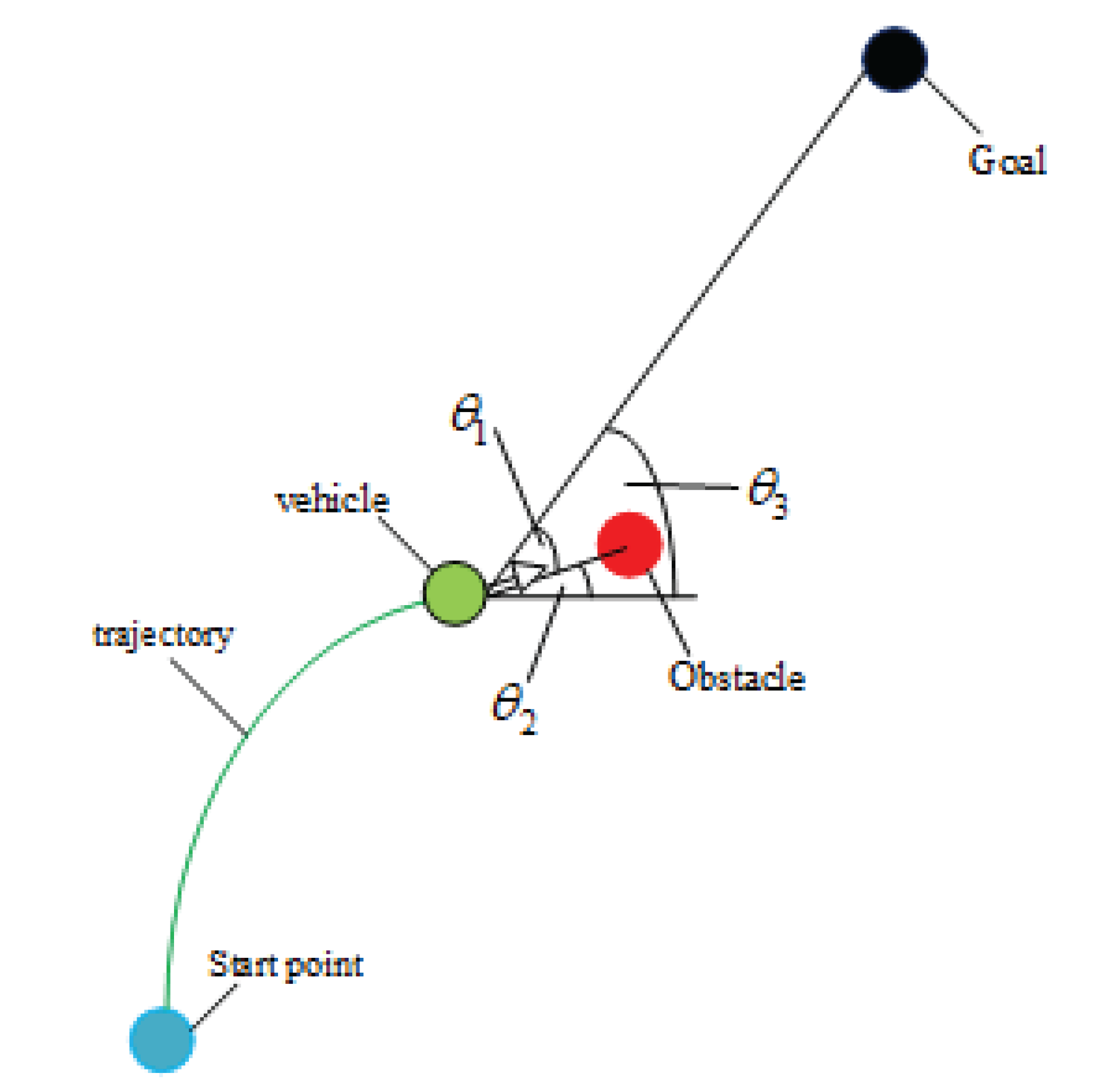
In the figure,${\theta }_1$ represents the angle between the line connecting the unmanned vehicle’s trajectory endpoint and the obstacle center and the line connecting the unmanned vehicle’s trajectory endpoint and the target point. ${\theta }_2$represents the angle between the line connecting the unmanned vehicle’s trajectory endpoint and the obstacle center and the horizontal line. ${\theta }_3$ represents the angle between the line connecting the unmanned vehicle’s trajectory endpoint and the target point and the horizontal line. ${\theta }_1$ can be used to assess the relationship between the unmanned vehicle, the target point, and the obstacle. If ${\theta }_1<\frac{\pi }{2}$, it indicates that the obstacle is between the unmanned vehicle and the target point. Define $D_{min}$as the minimum distance between the unmanned vehicle and the obstacle, and $D_s$as the braking distance. The following formula can be used to calculate it:

$$D_s={V_{curr}}^2/(2·\dot{v})$$

(6)

If$D_{min}>D_s$, it is determined that the unmanned vehicle can safely brake, and the collision risk is 0. If ${\theta }_1<\frac{\pi }{2}$ and $D_{min}<D_s$, there is a collision risk. In this case, the collision risk function is defined as:

$$risk{(v,\omega )}^{\prime }=\left\{\begin{array}{c}\left|{\theta }_1\right|\left|{\theta }_1\right|<\pi \hfill \\ \left|2\pi -{\theta }_1\right|\left|{\theta }_1\right|>\pi \hfill \end{array}\right.$$

(7)

Therefore, the final collision risk function is:

$$risk(v,\omega )=\left\{\begin{array}{c}0D_{min}>D_s\hfill \\ risk{(v,\omega )}^{\prime }{D}_{min}<D_s\hfill \end{array}\right.$$

(8)

At the same time, due to the integration with the A* algorithm, the nodes from global path planning need to be incorporated into the evaluation function. Therefore, the redesigned evaluation function is as follows:

$$G(v,\omega )=\alpha heading(v,\omega )+\sigma vel(v,\omega )+\beta dist\_s(v,\omega )+\gamma dist\_d(v,\omega )+\mu risk(v,\omega )$$

(9)

In the equation, $dist\_s(v,\omega )$represents the closest distance from the current trajectory endpoint to a known static obstacle, $dist\_d(v,\omega )$represents the closest distance from the current trajectory endpoint to an unknown obstacle, and $risk(v,\omega )$ represents the collision risk evaluation function.

2.3. Traditional A* Algorithm and Improvements

The A* algorithm, as a classic traditional path planning algorithm, demonstrates excellent performance in computing globally optimal paths and plays a crucial role in fields such as robot navigation. Serving as a fusion of Dijkstra’s algorithm and Breadth-First Search (BFS), A* incorporates the application of a heuristic function, which is a core feature of the algorithm. The evaluation function expression for A* algorithm is:

$$F\left(n\right)=G\left(n\right)+H\left(n\right)$$

(10)

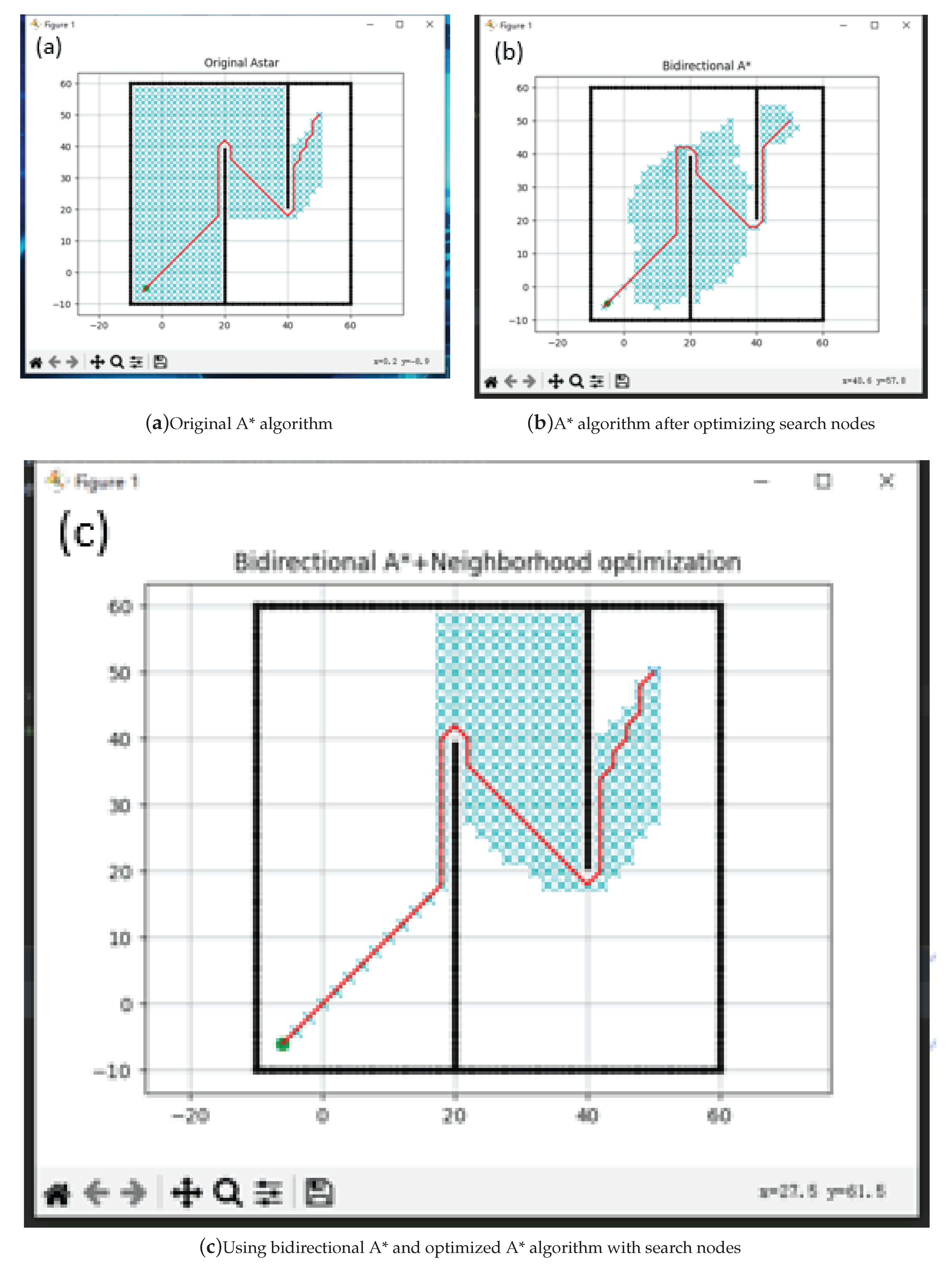
In the equation,$F\left(n\right)$represents the cost estimate from the start point to the target point, $G\left(n\right)$represents the cost from the start point to the current node, and $H\left(n\right)$ represents the cost estimate from the current node to the target node. The traditional A* algorithm may experience a decline in efficiency due to redundant searches of nodes, prompting this paper to optimize the search direction and evaluation function. Additionally, the bidirectional A* search method is employed to further enhance efficiency.

From the perspective of A* algorithm’s search nodes, the traditional approach involves examining nodes in all eight directions around the current node to ensure optimal solutions. However, for a fixed grid map and a fixed endpoint, this method increases the search space and reduces efficiency. Therefore, this paper reduces the number of search directions from eight to five.

Figure 3 represents the child nodes that the current node needs to search in the A* algorithm. It is evident that if the endpoint is to the right of the parent node at this point, child nodes 1, 7, and 8 do not need to be searched and can be directly discarded. It is not difficult to observe that the specific node to be discarded depends solely on the positions of the start and end points. Therefore, the specific discard rules are shown in the following table:

Figure 3. Child node diagram

Figure 3. Child node diagram

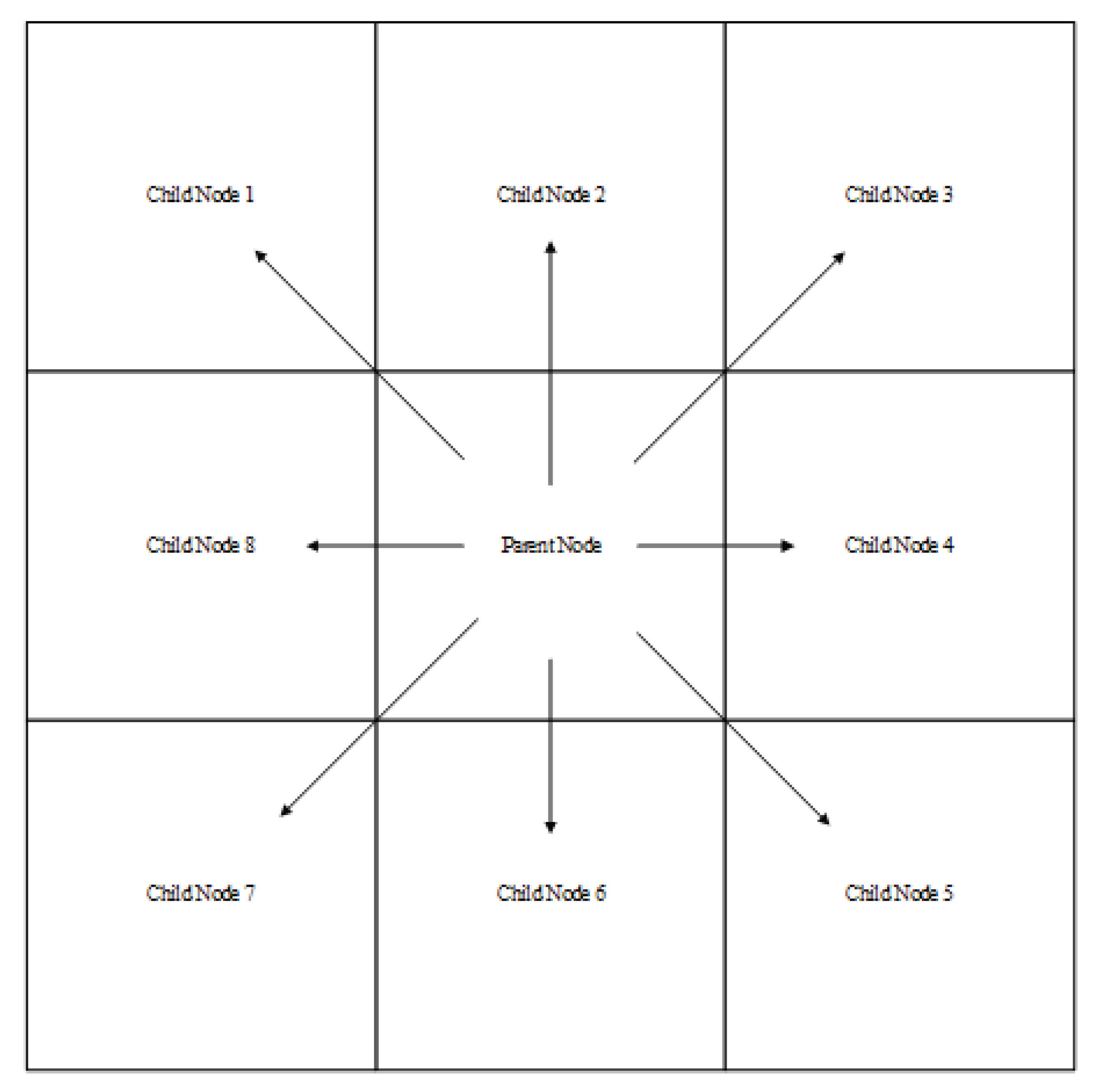
Table 1. Abandoning search direction rules.

$\mathit{\alpha }$	Reserved search directions	Discarded search direction
$\left(337.5,360\right]\cup \left(0,22.5\right]$	$$\begin{array}{c}\hfill 000\theta ,045\theta ,090\theta ,\hfill \\ \hfill 270\theta ,315\theta \hfill \end{array}$$	$\begin{array}{c}\hfill 135\theta ,180\theta ,\hfill \\ \hfill 225\theta \hfill \end{array}$
$\left(22.5,67.5\right]$	$\begin{array}{c}\hfill 000\theta ,045\theta ,090\theta ,\hfill \\ \hfill 135\theta ,315\theta \hfill \end{array}$	$\begin{array}{c}\hfill 180\theta ,225\theta ,\hfill \\ \hfill 270\theta \hfill \end{array}$
$\left(67.5,112.5\right]$	$\begin{array}{c}\hfill 000\theta ,045\theta ,090\theta ,\hfill \\ \hfill 135\theta ,180\theta \hfill \end{array}$	$\begin{array}{c}\hfill 225\theta ,270\theta ,\hfill \\ \hfill 315\theta \hfill \end{array}$
$\left(112.5,157.5\right]$	$\begin{array}{c}\hfill 045\theta ,090\theta ,135\theta ,\hfill \\ \hfill 180\theta ,225\theta \hfill \end{array}$	$\begin{array}{c}\hfill 270\theta ,315\theta ,\hfill \\ \hfill 000\theta \hfill \end{array}$
$\left(157.5,202.5\right]$	$\begin{array}{c}\hfill 090\theta ,135\theta ,180\theta ,\hfill \\ \hfill 225\theta ,270\theta \hfill \end{array}$	$\begin{array}{c}\hfill 000\theta ,045\theta ,\hfill \\ \hfill 315\theta \hfill \end{array}$
$\left(202.5,247.5\right]$	$\begin{array}{c}\hfill 135\theta ,180\theta ,225\theta ,\hfill \\ \hfill 270\theta ,315\theta \hfill \end{array}$	$\begin{array}{c}\hfill 000\theta ,045\theta ,\hfill \\ \hfill 090\theta \hfill \end{array}$
$\left(247.5,292.5\right]$	$\begin{array}{c}\hfill 180\theta ,225\theta ,270\theta \hfill \\ \hfill 315\theta ,000\theta \hfill \end{array}$	$\begin{array}{c}\hfill 045\theta ,090\theta ,\hfill \\ \hfill 135\theta \hfill \end{array}$
$\left(292.5,337.5\right]$	$\begin{array}{c}\hfill 225\theta ,270\theta ,315\theta \hfill \\ \hfill 000\theta ,045\theta \hfill \end{array}$	$\begin{array}{c}\hfill 090\theta ,135\theta ,\hfill \\ \hfill 180\theta \hfill \end{array}$

Table 1. Abandoning search direction rules.

$\mathit{\alpha }$	Reserved search directions	Discarded search direction
$\left(337.5,360\right]\cup \left(0,22.5\right]$	$$\begin{array}{c}\hfill 000\theta ,045\theta ,090\theta ,\hfill \\ \hfill 270\theta ,315\theta \hfill \end{array}$$	$\begin{array}{c}\hfill 135\theta ,180\theta ,\hfill \\ \hfill 225\theta \hfill \end{array}$
$\left(22.5,67.5\right]$	$\begin{array}{c}\hfill 000\theta ,045\theta ,090\theta ,\hfill \\ \hfill 135\theta ,315\theta \hfill \end{array}$	$\begin{array}{c}\hfill 180\theta ,225\theta ,\hfill \\ \hfill 270\theta \hfill \end{array}$
$\left(67.5,112.5\right]$	$\begin{array}{c}\hfill 000\theta ,045\theta ,090\theta ,\hfill \\ \hfill 135\theta ,180\theta \hfill \end{array}$	$\begin{array}{c}\hfill 225\theta ,270\theta ,\hfill \\ \hfill 315\theta \hfill \end{array}$
$\left(112.5,157.5\right]$	$\begin{array}{c}\hfill 045\theta ,090\theta ,135\theta ,\hfill \\ \hfill 180\theta ,225\theta \hfill \end{array}$	$\begin{array}{c}\hfill 270\theta ,315\theta ,\hfill \\ \hfill 000\theta \hfill \end{array}$
$\left(157.5,202.5\right]$	$\begin{array}{c}\hfill 090\theta ,135\theta ,180\theta ,\hfill \\ \hfill 225\theta ,270\theta \hfill \end{array}$	$\begin{array}{c}\hfill 000\theta ,045\theta ,\hfill \\ \hfill 315\theta \hfill \end{array}$
$\left(202.5,247.5\right]$	$\begin{array}{c}\hfill 135\theta ,180\theta ,225\theta ,\hfill \\ \hfill 270\theta ,315\theta \hfill \end{array}$	$\begin{array}{c}\hfill 000\theta ,045\theta ,\hfill \\ \hfill 090\theta \hfill \end{array}$
$\left(247.5,292.5\right]$	$\begin{array}{c}\hfill 180\theta ,225\theta ,270\theta \hfill \\ \hfill 315\theta ,000\theta \hfill \end{array}$	$\begin{array}{c}\hfill 045\theta ,090\theta ,\hfill \\ \hfill 135\theta \hfill \end{array}$
$\left(292.5,337.5\right]$	$\begin{array}{c}\hfill 225\theta ,270\theta ,315\theta \hfill \\ \hfill 000\theta ,045\theta \hfill \end{array}$	$\begin{array}{c}\hfill 090\theta ,135\theta ,\hfill \\ \hfill 180\theta \hfill \end{array}$

In the table, $\alpha$ represents the included angle between the line connecting the starting point and the point and the true north direction, $315\theta$ represents the child node 1, $000\theta$ represents the child node 2, $045\theta$ represents the child node 3, $090\theta$ represents the child node 4, $135\theta$ represents the child node 5, $180\theta$ represents the child node 6, $225\theta$ represents the child node 7, and $270\theta$ represents the child node 8.

According to equation (10), when $H\left(n\right)$ is 0, the algorithm degenerates into the Dijkstra algorithm. When $H\left(n\right)$ is always less than or equal to the cost of node n to the endpoint, the A * algorithm ensures that it can always find the shortest path. But the smaller the value of $H\left(n\right)$, the more nodes the algorithm will traverse, which leads to a slower algorithm. When $H\left(n\right)$ is completely equal to the cost of node n to the endpoint, the A * algorithm will find the best path. When the value of $H\left(n\right)$ is greater than the cost of node n to the endpoint, the A * algorithm cannot guarantee finding the shortest path. Therefore, this article introduces weights into the evaluation function and controls the size of $H\left(n\right)$ through dynamic weights to ensure search efficiency. The evaluation function is optimized to:

$$F\left(n\right)=G\left(n\right)+(1+r/R)*H\left(n\right)$$

(11)

In the formula, r represents the distance from the current node to the target point, and R represents the distance from the starting point to the target point. Through equation (11), it can be seen that as the distance approaches the target point, the weight of the heuristic function $H\left(n\right)$ increases, and the algorithm traverses fewer nodes, resulting in improved efficiency.

Meanwhile, this article uses a bidirectional A * method to improve the efficiency of the A * algorithm and reduce planning time. The specific and brief steps are as follows:

• Using the dual A * algorithm, become A1 and A2 respectively;
• A1 starts from the starting point, A2 starts from the endpoint;
• A1 extends to the grid with the smallest F value in the open table of A2 as the endpoint;
• A2 extends to the grid with the smallest F value in the open table of A1 as the endpoint;
• If the open tables of A1 and A2 are empty, it means there is no path, exit;
• Repeat (3), (4), and (5) until A1 and A2 meet, indicating successful path finding and exit.

3. Algorithm Fusion

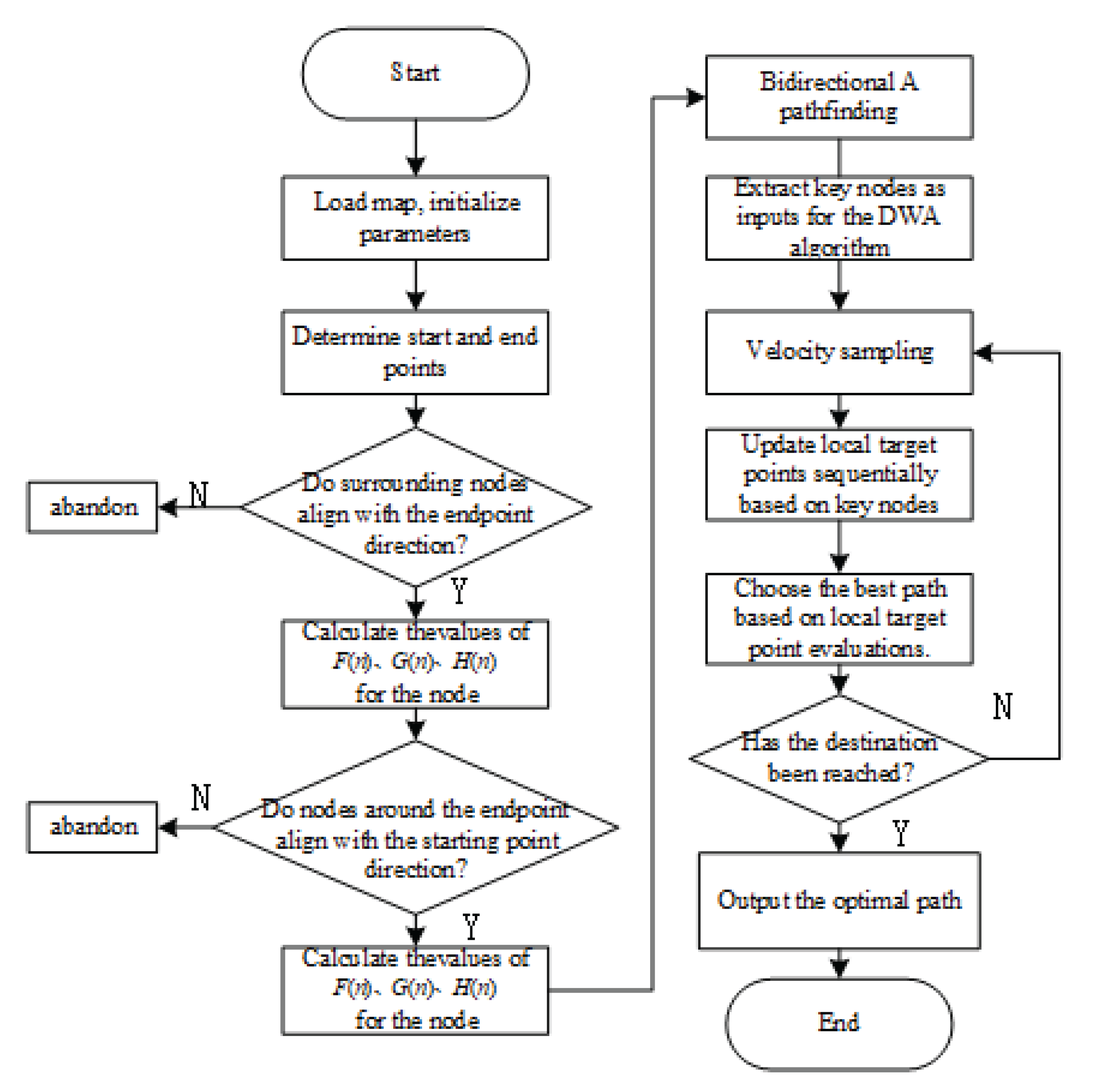
Due to the respective shortcomings of both A * algorithm and DWA algorithm, A * algorithm is undoubtedly excellent for global path planning. However, for a well planned path, sudden unknown obstacles often cannot be avoided. DWA algorithm can avoid unknown obstacles well, but it is easy to fall into the dilemma of local optima. This article combines the above two methods by using the path key points of the A * algorithm as temporary endpoints for the DWA algorithm. The fused algorithm can avoid unknown and dynamic obstacles. The algorithm flowchart is as follows.

Figure 4. Fusion algorithm process

Figure 4. Fusion algorithm process

4. Simulation

4.1. Comparative Experiment on Improving A* Algorithm

Figure 5. Path under the same A* algorithm

Figure 5. Path under the same A* algorithm

4.2. Comparative Experiment on Improving DWA Algorithm

Figure 6. Comparison of evaluation function before and after modification

Figure 6. Comparison of evaluation function before and after modification

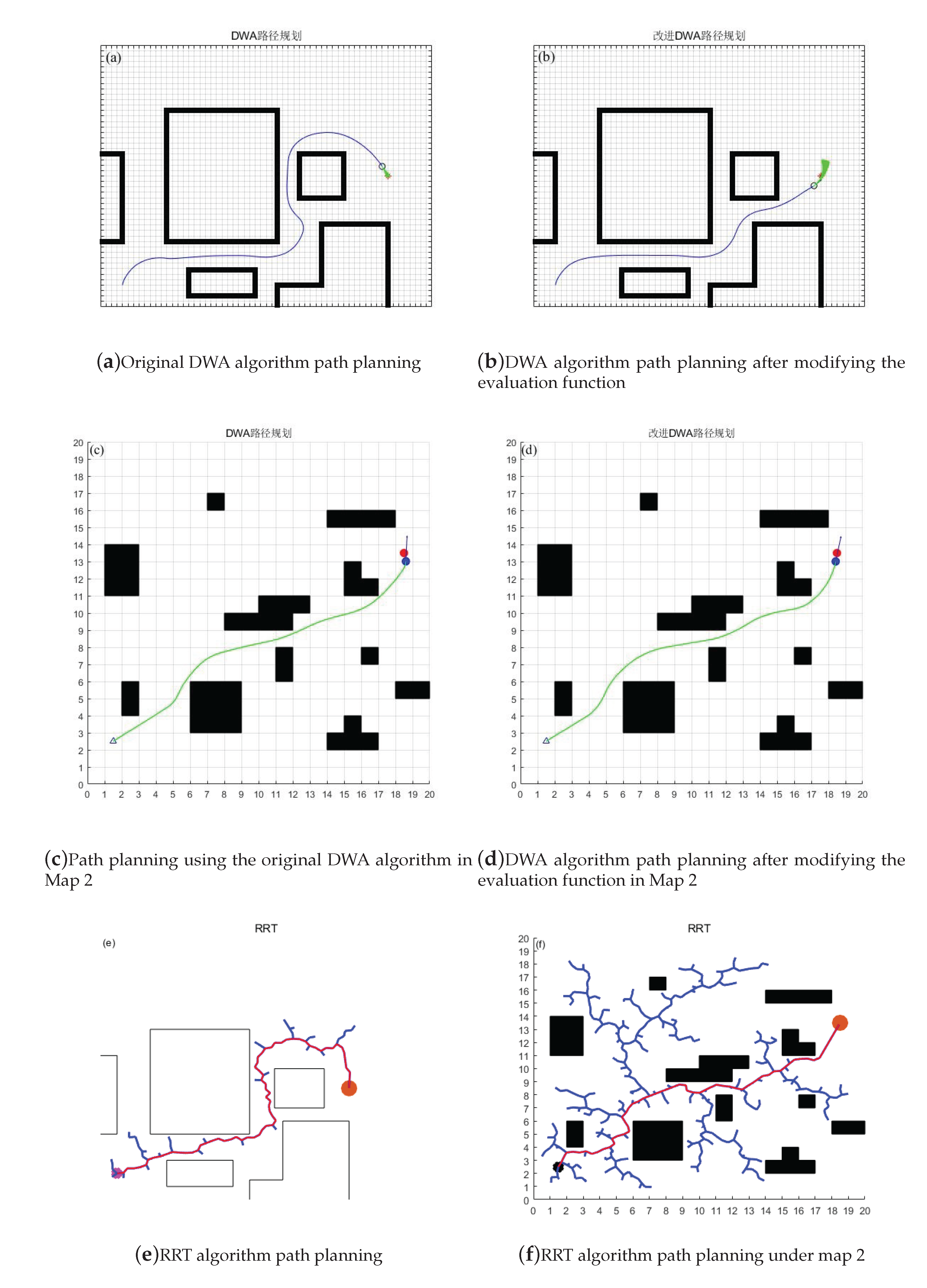
Through the comparison of experiments before and after improvement, it can be seen that the improved algorithm has better path selection and shorter distance in Map 1. In Map 2, it has a longer distance from obstacles and can retain a larger braking distance to avoid collision with obstacles. However, through the comparison of experiments between DWA algorithm and RRT algorithm, it can be found that the path planned by RRT algorithm is not smooth and accompanied by steep turns, This is more dangerous for faster speeds, and through the comparison of Map 1 and Map 2 with the DWA algorithm, our improved algorithm has a smoother path and safer distance against obstacles. The specific experimental data are shown in Table 2 to Table 3.

Table 2. Experimental data in Map 1.

Algorithm	Nodes	Time(t)	Average linear velocity(m/s)	Length(m)	iterations
Original DWA algorithm	560	206.48	0.294	60.748	170
RRT algorithm	480	185.63	0.308	57.174	195
Improved DWA	460	172.82	0.321	55.474	205

Table 2. Experimental data in Map 1.

Algorithm	Nodes	Time(t)	Average linear velocity(m/s)	Length(m)	iterations
Original DWA algorithm	560	206.48	0.294	60.748	170
RRT algorithm	480	185.63	0.308	57.174	195
Improved DWA	460	172.82	0.321	55.474	205

Table 3. Experimental data in Map 2.

Algorithm	Nodes	Time(t)	Average linear velocity(m/s)	Length(m)	iterations
Original DWA algorithm	330	169.22	0.228	38.583	149
RRT algorithm	280	141.23	0.254	35.873	156
Improved DWA	240	121.66	0.283	34.431	165

Table 3. Experimental data in Map 2.

Algorithm	Nodes	Time(t)	Average linear velocity(m/s)	Length(m)	iterations
Original DWA algorithm	330	169.22	0.228	38.583	149
RRT algorithm	280	141.23	0.254	35.873	156
Improved DWA	240	121.66	0.283	34.431	165

4.3. Comparison Experiment of Fusion Algorithms

Figure 7. Comparison of path planning before and after fusion algorithm improvement

Figure 7. Comparison of path planning before and after fusion algorithm improvement

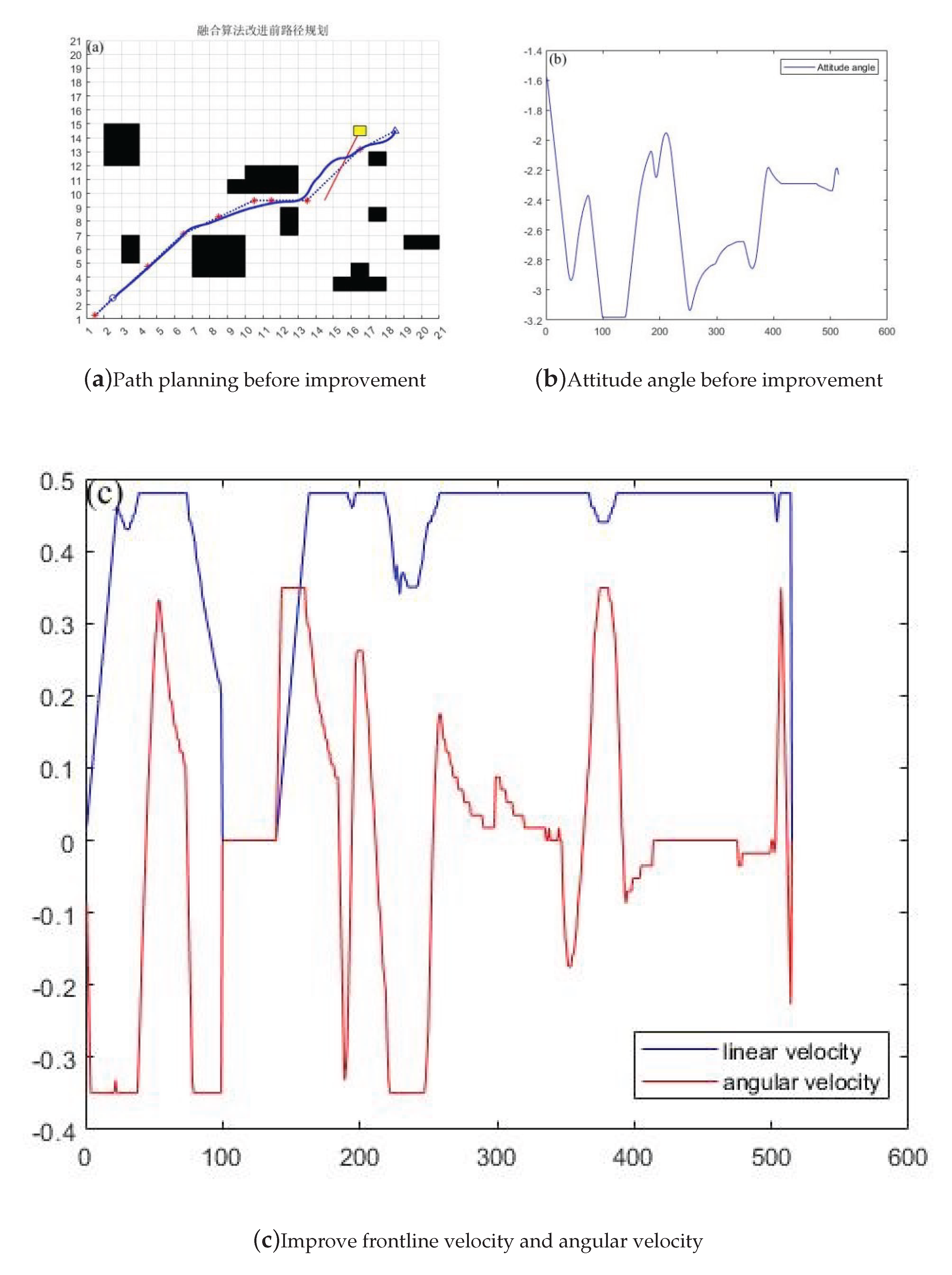
Figure 8. Path planning after improved fusion algorithm

Figure 8. Path planning after improved fusion algorithm

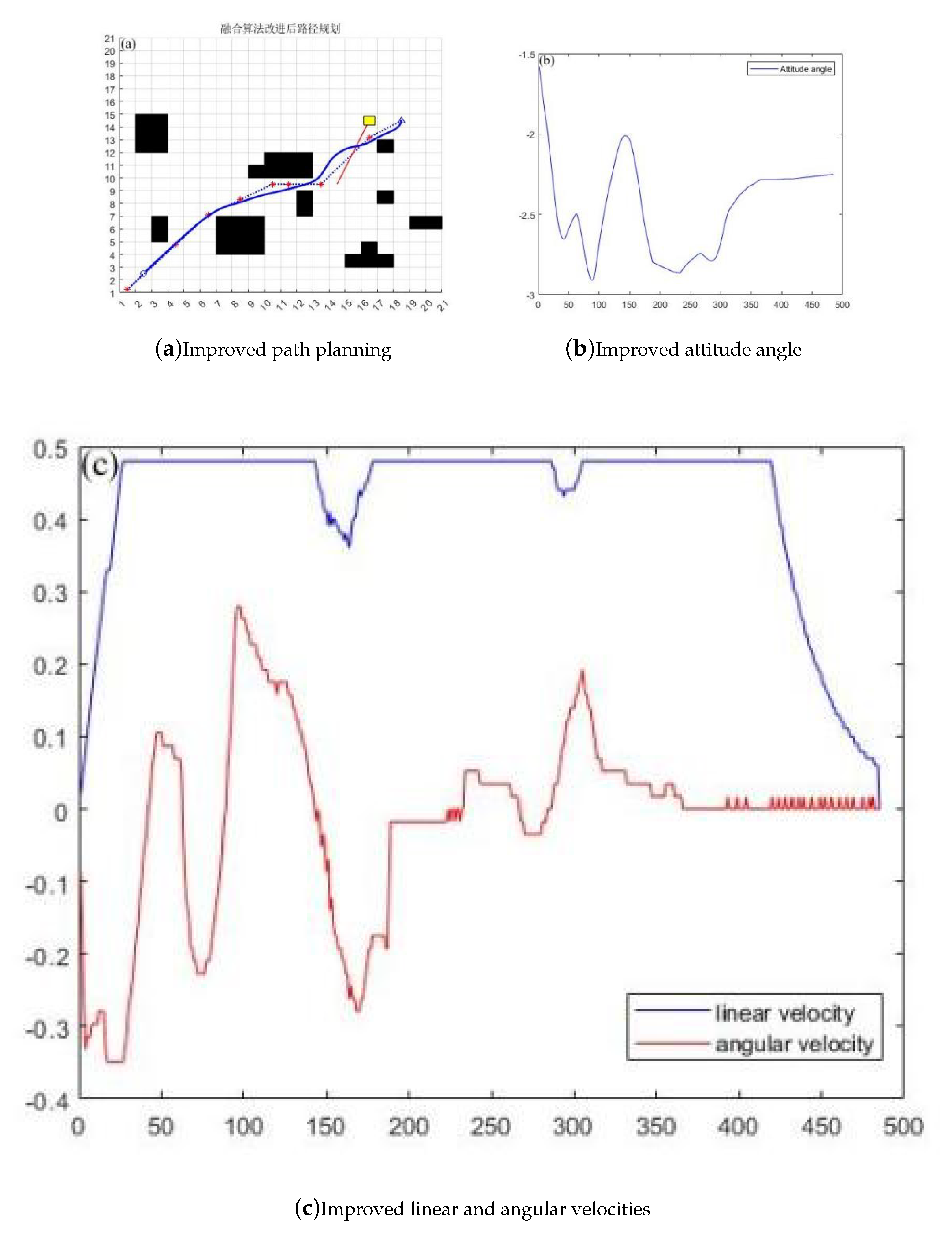
Table 4. Experimental data before and after fusion algorithm improvement.

Algorithm	Nodes	Time(t)	Average linear velocity(m/s)	Length(m)	iterations
Before Improvement	340	169.22	0.439	74.288	149
Improved	300	157.51	0.452	71.195	165

Table 4. Experimental data before and after fusion algorithm improvement.

Algorithm	Nodes	Time(t)	Average linear velocity(m/s)	Length(m)	iterations
Before Improvement	340	169.22	0.439	74.288	149
Improved	300	157.51	0.452	71.195	165

5. Conclusions

This article analyzes the advantages and disadvantages of path planning using traditional A * and DWA algorithms, and proposes a method for integrating the improved A * and DWA algorithms. According to the simulation results and data, the new fusion algorithm reduces time by 11.71 seconds, a year-on-year decrease of 6.9%, a path length reduction of 3.093 meters, a year-on-year decrease of 4.16%, and an average linear speed increase of 2.9%. It can be seen that, The efficiency and path length of the improved algorithm after fusion have been optimized to a certain extent. At the same time, the line speed has increased, indicating that the vehicle can complete the task objectives at higher speeds. At the same time, through experimental data graphs, it can be seen that the vehicle can better judge the path of obstacles ahead and will not detour, and the path is smoother compared to the RRT algorithm and the fusion improvement.

References

- Jasika, N.; Alispahic, N.; Elma, A.; Ilvana, K.; Elma, L.; Nosovic, N. Dijkstra’s shortest path algorithm serial and parallel execution performance analysis. 2012 Proceedings of the 35th International Convention MIPRO, 2012, pp. 1811–1815.
- Hart, P.E.; Nilsson, N.J.; Raphael, B. A formal basis for the heuristic determination of minimum cost paths. IEEE transactions on Systems Science and Cybernetics 1968, 4, 100–107. [Google Scholar] [CrossRef]
- Duchoň, F.; Babinec, A.; Kajan, M.; Beňo, P.; Florek, M.; Fico, T.; Jurišica, L. Path planning with modified a star algorithm for a mobile robot. Procedia engineering 2014, 96, 59–69. [Google Scholar] [CrossRef]
- ZHAO Xiao, WANG Zheng, H.C.; Yanwei, Z. Mobile Robot Path Planning Based on an Improved A* Algorithm. ROBOT 2018, 40. [CrossRef]
- Wang, D. Indoor mobile-robot path planning based on an improved A* algorithm. Journal of Tsinghua University Science and Technology 2012, 52, 1085–1089. [Google Scholar]
- Wen, Z.; Yong, L.; Chaofan, Z.; Long, Z.; Yingwei, X. Real-time Path Planning of Greenhouse Robot Based on Directional A* Algorithm. Nongye Jixie Xuebao/Transactions of the Chinese Society of Agricultural Machinery 2017, 48. [Google Scholar]
- Trovato, K.I.; Dorst, L. Differential a. IEEE Transactions on Knowledge and Data Engineering 2002, 14, 1218–1229. [Google Scholar] [CrossRef]
- CHENG Chuanqi, HAO Xiangyang, L.J.Z.Z.; Guopeng, S. Global Dynamic Path Planning Based on Fusion of Improved A* Algorithm and Dynamic Window Approach. Journal of Xi’an Jiaotong University 2017, 51.
- Wang Xiaohong, Y.T. Research on Robot Path Planning Based on Improved A* Algorithm. Computer Measurement & Control 2018, 26. [Google Scholar] [CrossRef]
- Fox, D.; Burgard, W.; Thrun, S. The dynamic window approach to collision avoidance. IEEE Robotics & Automation Magazine 1997, 4, 23–33. [Google Scholar]
- Seder, M.; Petrovic, I. Dynamic window based approach to mobile robot motion control in the presence of moving obstacles. Proceedings 2007 IEEE International Conference on Robotics and Automation. IEEE, 2007, pp. 1986–1991.
- Tuvshinjargal, D.; Dorj, B.; Lee, D.J.; others. Hybrid motion planning method for autonomous robots using kinect based sensor fusion and virtual plane approach in dynamic environments. Journal of Sensors 2015, 2015.
- Xiong, W.; Yong, T.; Xuan, L.; Hua, L. Adaptive dynamic window method for crossing dense obstacles. Control Decis Mak 2019, 34, 927–936. [Google Scholar]
- Jinping, L. Robot path plan ning of Autonomous Walking and Space Operation. Master’s thesis, Xidian University, 2021.
- CHANG Xinxin, HU Wei, J.S.; Yumei, Y. Obstacle Avoidance of Mobile Robot Based on Improved Dynamic Window Method. Modular Machine Tool & Automatic Manufacturing Technique 2021. [CrossRef]
- Xin, L.; Huanhuan, Y. A Path Planning Method for EOSID Based on Dynamic Window Approach. Journal of Civil Aviation Flight University of China 2021, 32. [Google Scholar]
- Haohan, S. Research on Path Planning of Tracked Unmanned Platform in Dynamic Environment. Master’s thesis, Harbin Institute of Technology, 2020.
Disclaimer/Publisher’s Note: The statements, opinions and data contained in all publications are solely those of the individual author(s) and contributor(s) and not of MDPI and/or the editor(s). MDPI and/or the editor(s) disclaim responsibility for any injury to people or property resulting from any ideas, methods, instructions or products referred to in the content. |
© 2024 by the authors. Licensee MDPI, Basel, Switzerland. This article is an open access article distributed under the terms and conditions of the Creative Commons Attribution (CC BY) license (http://creativecommons.org/licenses/by/4.0/).
Copyright: This open access article is published under a Creative Commons CC BY 4.0 license, which permit the free download, distribution, and reuse, provided that the author and preprint are cited in any reuse.