Submitted:
28 March 2024
Posted:
29 March 2024
You are already at the latest version
Abstract
The term "code smell" refers to an indication of a problem with the quality of source code. Numerous studies have been conducted to identify problematic features in source code. Initially, the focus was on utilizing metric-based and heuristic-based approaches. In recent years, however, there has been a shift towards using machine learning and deep learning (DL) techniques for smell detection. Nevertheless, the current algorithms are still considered to be in the early stages of development. Recognizing the challenges associated with identifying smells using DL methods, both academics and software developers have made efforts to address these obstacles. This work involves constructing and evaluating new DL models for code smell detection. Two models are built upon stacked autoencoders, employing a hybrid architecture that combines bidirectional long short-term memory and convolutional neural network components.
Keywords:
machine learning
; deep learning
; stack auto encoder
; code smell detection
; auto encoder.
1. Introduction
In software development and programming, a characteristic present in the source code that could potentially lead to bugs, vulnerabilities, or other unwanted issues is referred to as a “code smell.” While not a direct bug, it has the potential to cause problems. Code smell patterns vary across programming languages, developer coding standards, standard coding practices, and development methodologies [2].
As the software industry rapidly grows, companies must frequently update the code bases of their software or solutions to remain competitive in the market. However, the existence of code smells within their code base can make scaling difficult, potentially resulting in significant financial and reputational losses for the software industry [3].
Major instances of technical debt include code smells and ineffective design decisions made by developers, which can have a negative impact on the maintainability, scalability, and quality of a software system [4]. Over the past few decades, research has heavily focused on the following areas [5]:
- The evolution of code smells.
- The definition of code smells.
- The understanding, interest, and ability of software development teams to fix code smells.
- The effect on source code before and after fixing code smells.
Code smells are categorized into different types based on the kind of bugs they can potentially cause. Here are some of the most common code smells [6]: long method, divergent change, parallel inheritance hierarchies, lazy class, incomplete library class, speculative generality, middleman, shotgun surgery, feature envy, long parameter list, comments, message chains, data clumps, inappropriate intimacy, large class, dead code, duplicate code, data class, object-orientation abusers, etc.
Code smells are software defects that can potentially lead to issues in maintaining and evolving the software [27]. They are interconnected within a software system rather than appearing as isolated instances [28]. This means that code smells are not limited to individual classes or methods, but they exist and interact among various classes and methods [29]. For example, if a class calls a method of another class, the called method or the way it is called can be considered smelly. These clusters of software problems cause difficulties in maintaining the software, especially during updates, upgrades, and evolution.
The problems that affect the overall quality of software, commonly referred to as code smells, can take the form of poorly designed architecture, hidden bugs, misuse of design patterns, or badly written code [4]. These code smells hinder the evolution of the software itself. When software cannot evolve, it becomes significantly expensive for the software industry to rebuild it from scratch. In the software engineering industry, extensive research has been conducted to identify code smells within codebases during software development and investigate their impact and various dimensions. Rule-based or static code analysis tools are increasingly popular [5]. By using intelligent code smell analysis and detection systems, the system would be able to adapt and update rules and sequences based on new changes, enabling it to predict or identify code smells in advance [6]. While many rule-based code analysis tools evaluate code based on predefined rules, they may struggle to incorporate new coding, design, or implementation standards. New rules need to be developed and implemented [7].
Currently, there are numerous machine learning (ML) techniques being researched for code smell detection, including decision trees (DTs) [8], support vector machines (SVMs) [9], random forests [10], J48 [11], JRip [12], naïve Bayes, k-nearest neighbor (KNN), and logistic regression (LR) [13]. Although these ML approaches show promise, it is important to note that they still have limitations. It can be inferred that ML approaches for detecting code smells represent one of the most intriguing research areas, but challenges remain.
2. Related Works
Several approaches to detecting code smells have been proposed in recent years.
Fontan et al. (2016) [14] conducted an experiment using 16 different ML algorithms. The study focused on four types of code smells: Data class, large class, feature envy, and long method. A total of 74 software systems were analyzed, and 1,986 instances of code smells were manually confirmed. The researchers found that all algorithms performed exceptionally well on the cross-validation dataset. However, J48 and random forest showed the highest levels of performance, while SVMs performed the worst. Nevertheless, due to the relatively low occurrence of code smells, resulting in imbalanced data across the dataset, the performances were inconsistent and should be explored further in future research. The researchers concluded that using ML to identify these code smells can achieve a high level of accuracy (>96%), but a minimum of one hundred training examples is required to achieve at least 95% accuracy.
In their 2019 study, Mhawish and Gupta [15] introduced an approach based on ML aimed at identifying code smells in software. They thoroughly analyzed important metrics crucial to the detection process and used two feature selection strategies that leveraged genetic algorithms. Additionally, they fine-tuned parameters using a grid search method. Their GA_CFS approach demonstrated remarkable accuracy rates in detecting various code smells, achieving scores of 98.05%, 97.56%, and 94.31% for data class, god class, and long method, respectively. Furthermore, their GA-naïve Bayes feature selection method excelled with an accuracy rate of 98.38%, particularly in identifying long-method smells.
In another study from 2019, Baarah et al. [16] explored eight machine learning techniques (MLTs) to assess the significance of software bugs reported in closed-source projects. These bugs were associated with numerous proprietary projects developed by the INTIX corporation in Amman, Jordan. Utilizing data from the JIRA bug monitoring system, they found that the DT approach consistently outperformed other MLTs.
Pushpalatha et al. (2019) [17] proposed a method for predicting the severity of bug reports within closed-source datasets. They obtained their dataset (PITS) from NASA programs via the PROMISE database. By employing ensemble methods and two-dimensional reduction strategies—specifically Chi-square and information gain—they significantly enhanced accuracy. Their findings revealed that their proposed model outperformed other algorithms tested, achieving accuracy rates ranging from 79.85% to 89.80%.
In their 2020 study, Pecorelli et al. [18] examined five strategies aimed at addressing issues with imbalanced data and evaluated their impact on MLTs used to detect code smells in object-oriented applications, including those following the model–view–controller design. Contrary to expectations, our research indicates that not addressing imbalanced data does not significantly affect accuracy. However, current techniques for balancing data are found to be inadequate for effectively detecting code smells, leading to low accuracy in ML-based methods. Therefore, there is a pressing need for novel measures that leverage diverse software attributes and innovative approaches to integrate them efficiently.
Guggulothu and Moiz (2020) [19] investigated the detection of code smells using a multi-label classification approach. They utilized this technique to determine if provided code elements are influenced by multiple odors, employing an unsupervised classification methodology to achieve high accuracy. Notably, they achieved a maximum accuracy of 99.10% using the B-J48 pruned algorithm on the feature-envy dataset and a maximum accuracy of 95.90% using the Random Forest methodology on the long-method dataset.
In 2021, Draz et al. [20] proposed a search-based approach to enhance code smell prediction by utilizing the whale optimization method as a classifier. Conducting their experiment on five open-source programs, they identified nine different types of code smells, achieving an average precision of 94.24% and a recall of 93.4%.
Liu et al. (2021) [21] introduced a novel deep learning (DL) method for detecting code smells. They utilized deep neural networks with advanced DL algorithms to automatically identify aspects of source code during smell detection. They emphasized a key challenge in utilizing DL for smell detection, which often depends on large quantities of labeled training data to optimize several parameters in the deep neural network. As current datasets for code smell detection are limited, they proposed an automated method for generating annotated training data for the classifier using neural networks, without human involvement. Their preliminary implementation of this approach on four prevalent code smells—feature envy, long method, huge class, and misplaced class—showed promising results, outperforming state-of-the-art techniques.
In 2021, Yadav et al. [22] presented a model for detecting code smells based on a DT method. They used two datasets for code smells, blob-class and data-class, obtained from Fontana et al., which were compiled from 74 different open-source systems. To evaluate the performance of the DT model on each dataset, they employed fivefold cross-validation. This involved dividing the datasets into training and testing sets, and further splitting the training set into two parts for training and validation. By utilizing grid search for hyper-parameter tuning and decision rule extraction, they achieved the highest accuracy of 97.62% for both classes.
In 2021, Gupta et al. [23] proposed using feature extraction from source code to predict eight different types of code smells. They addressed the issue of class imbalance by employing a data sampling strategy and conducted feature selection to identify the most relevant feature sets. By leveraging DL techniques, they improved the accuracy of the Area Under the Curve from 88.47% to 96.84%.
In 2022, Dewangan and Rao [24] presented several ML models for detecting code smells across four code smell datasets. They used a feature selection method to choose the best features in the dataset and applied ten-iteration cross-validation to evaluate the performance of the predicted model. The results showed that the random forest model achieved the highest accuracy for detecting feature-envy code smells, with an accuracy of 99.12%.
3. Methodology
An auto-associative neural network (autoencoder) is a specific instance of a multi-layer perceptron network (MLP) where the number of neurons in the input layer is the same as the number of neurons in the output layer. This type of neural network is trained to perform the identity function, mapping the input patterns to the output. Figure 1 depicts the structure of an autoencoder.
The autoencoder network maps inputs from space (external environment) to space (internal), approximating a function , and obtains the inverse mapping from S’ to (network output), approximating the inverse function . This process is called encoding and decoding information. If the output vector equals the input vector, all information flows through the bottleneck of S and is recomposed in S’. Thus, the autoencoder learns the real data and stores it in its weights. The intermediate layer of the autoencoder network is responsible for extracting features from the information provided by the input neurons. This layer enables the network to store only knowledge related to the main characteristics of the problem’s dataset. Therefore, the hidden layer encodes the data while the output layer reconstructs the original inputs, allowing the network to approximate the identity function. To train an autoencoder network, the standard Backpropagation algorithm is used. It is a special case of an MLP network, with minimization of the mean squared error between the values of the input and output neurons. Training is conducted in an unsupervised manner, as the goal of an ANN autoencoder is to minimize the error between its input sample and the output reconstruction, rather than minimizing the error between the output and an external label.
On the other hand, there is a type of architecture called stacked autoencoder (SAE), which includes an output layer where the activation function (such as SoftMax) is applied. The structure can be seen in Figure 2. In an SAE, autoencoder networks are connected, where the output signal from the hidden layer of one autoencoder (features extracted from the input applied to this autoencoder) serves as an input signal to another autoencoder. Finally, there is the layer responsible for classification, which uses the activation function to receive the signal extracted by the hidden layer of the last SAE as input. The use of SAE networks aims to extract characteristics from the original database so that they can be used for the classification problem through the activation function in the network output. Figure 2 shows the SAE model.
The activation function transforms the corresponding outputs for each class into values between zero and one by dividing them by the sum of the outputs. This essentially generates the probability of the input being in a certain class. For SoftMax, the function is defined as follows:
3.1. Proposed Model Structure
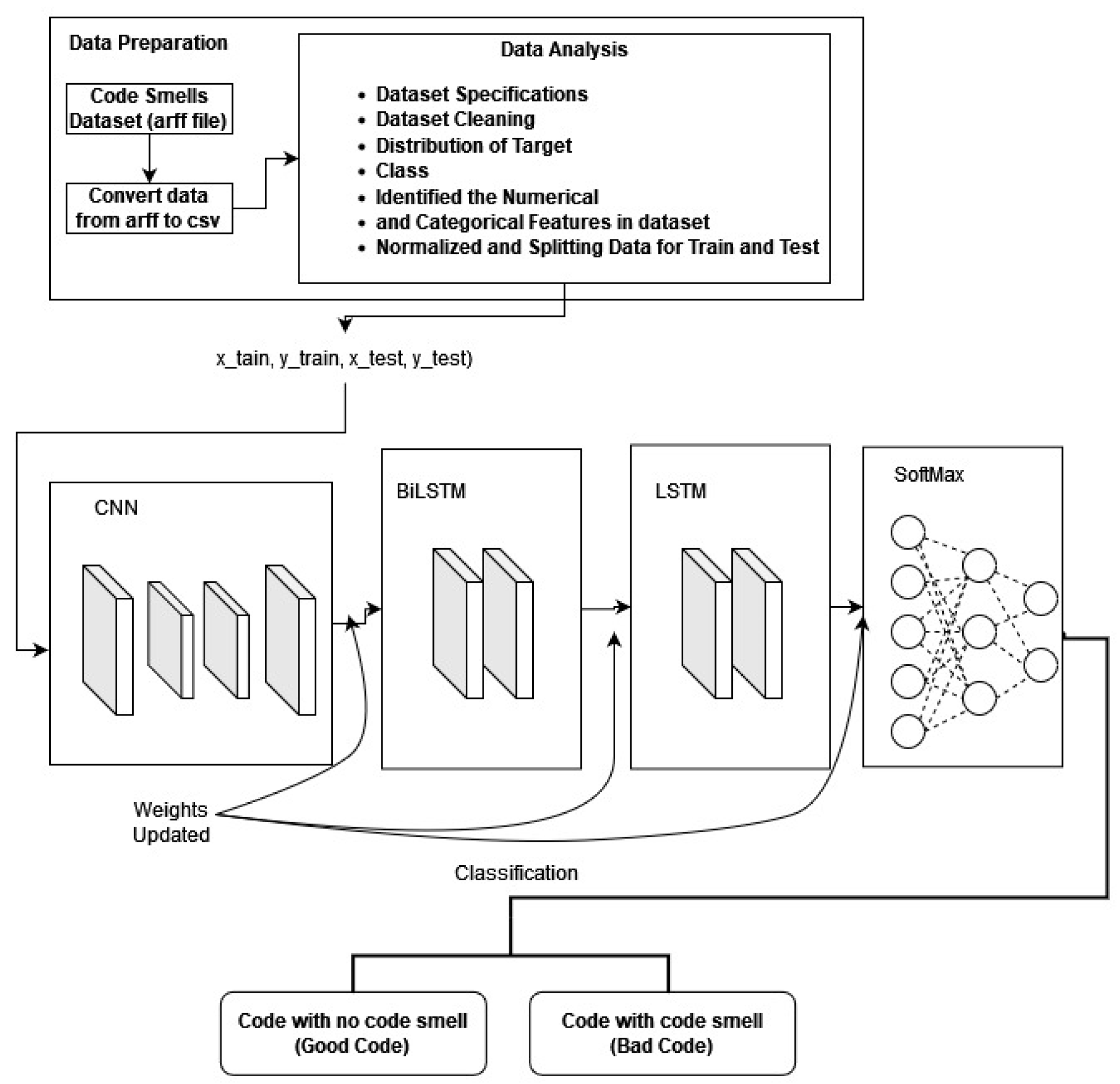
3.1.1. First Model (3-Layer Stacked CNN-BiLSTM-LSTM)
The proposed model includes an input layer, a permute layer, four 1D convolutional layers, two bidirectional long short-term memory (BiLSTM) layers, two long short-term memory (LSTM) layers, a concatenate layer, a dropout layer, and a dense layer. This convolutional neural network (CNN) architecture encompasses various functional layers such as convolution, pooling, and rectified linear unit (ReLU). The convolutional layer efficiently extracts sequential features inherent in time series data, which are crucial for analysis. Pooling layers facilitate downsampling in CNNs, while the permutation layer generates band combinations used by the CNN to create robust classification features. The concatenate layer is essential for multitask learning, as it integrates results from multiple layers into a single tensor. This integration is particularly beneficial for combining features learned from various activities, enhancing performance by leveraging shared characteristics across tasks. Moreover, using concatenate layers for training multitask models improves training efficiency by reducing the number of parameters and training duration. This efficiency arises from shared layer utilization, allowing the model to acquire knowledge from multiple tasks simultaneously. Additionally, the incorporation of concatenate layers enhances the model’s ability to generalize to new data instances by capturing common characteristics across tasks. By leveraging knowledge from diverse activities, the model becomes better equipped to tackle novel problems exhibiting similarities to those it was trained on.
The proposed Model 1, a 3-layer stacked CNN-BiLSTM-LSTM with an autoencoder structure, is described as follows:
- Layer 1: Input layer
- Layer 2 (permutes layer): Used to permute the dimensions of the input.
- Layer 3 (convolutional 1D layer): Consists of 128 filters with a kernel size of 3 and padding of 1. This layer reads input data from the input layer (layer 1) and sends outputs to convolutional layer (layer 5).
- Layer 4 (convolutional 1D layer): Has 128 filters with a kernel size of 3 and padding of 1, this layer reads input data from the permutes layer (layer 2) and sends output to convolutional layer (layer 6).
- Layer 5 (convolutional 1D layer): Has 64 filters with a kernel size of 1 and padding of 1. This layer mirrors layer 5 and reads input data from convolutional layer (layer 3), sending output to BiLSTM Layer (layer 7).
- Layer 6 (convolutional 1D layer): Has 64 filters with a kernel size of 1 and padding of 1. This layer also reads input data from convolutional layer (layer 3) and sends output to BiLSTM Layer (Layer 8).
- Layer 7 (BiLSTM layer): Contains 128 filters, serving as the integrated layer for convolutional layer 5. It reads input data from convolutional layer (Layer 5) and sends output to LSTM layer (Layer 9).
- Layer 8 (BiLSTM layer): Consists of 128 filters and serves as the integrated layer for convolutional layer 6. It reads input data from convolutional layer (layer 6) and sends output to LSTM layer (layer 9).
- Layer 9 (LSTM layer): Comprises 128 filters, serving as the integrated layer for BiLSTM layer 7. It reads input data from the BiLSTM layer (layer 7) and sends output to concatenate layer (layer 11).
- Layer 10 (LSTM layer): Contains 128 filters and serves as the integrated layer for BiLSTM layer 7. It reads input data from the BiLSTM layer (layer 8) and sends output to concatenate layer (layer 11).
- Layer 11 (encoded columns): A concatenate layer used to create a dense feature map. It concatenates the feature maps obtained from LSTM layers (layer 9 and layer 10) and passes them to dropout layer (layer 12).
- Layer 12 (dropout layer): Applies a dropout rate of 20% to encoded columns (layer 11) to prevent overfitting by randomly setting 20% of the input units to 0 during training.
- Layer 13 (dense layer): A fully connected layer where neurons receive inputs from layer 11 and predict class probabilities for each input sample. This layer utilizes the SoftMax activation function in model 1.
Figure 3.
Structure of 3-layer stacked CNN-BiLSTM-LSTM model.
3.1.2. Second Model (2-Layer Stacked CNN-BiLSTM)
In the second model, our goal is to simplify the first model by using a dual-layer SAE DL architecture to classify code smells. The detection algorithms focus on identifying code smells by extracting relevant features from the code dataset. We combined a BiLSTM and CNN within an SAE structure. In the CNN-SAE component, the encoder consists of a series of Conv2D with MaxPooling2D layers, where the MaxPooling2D layers are used for spatial downsampling. On the other hand, the decoder consists of a series of Conv2D with UpSampling2D layers. Figure 4 illustrates an autoencoder with two encoders stacked on top of each other.
The proposed BiLSTM-CNN autoencoder structure is described as follows:
- Layer 1: Input layer (60, 1)
CNN-SAE
A. Encoder
- Layer 2: Convolutional 1D layer with 128 filters, 3 kernel sizes, 1 padding, and ReLU activation function. Outputs 60 features.
- Layer 3: Max pooling 1D layer with 2 pool sizes and 1 padding. Outputs a feature vector, reducing dimension to 30.
- Layer 4: Convolutional 1D layer with 128 filters, 3 kernel sizes, 1 padding, and ReLU activation function. Outputs 30 features.
- Layer 5 (encoder): Max pooling 1D layer with 2 pool sizes and 1 padding. Encodes the feature vector to reduce dimension to 15.
B. Decoder
- Layer 6: Convolutional 1D layer with 128 filters, 3 kernel sizes, 1 padding, and ReLU activation function. Outputs 15 features.
- Layer 7: Max pooling 1D layer with 2 pool sizes and 1 padding. Outputs a feature vector.
- Layer 8: Convolutional 1D layer with 128 filters, 3 kernel sizes, 1 padding, and ReLU activation function. Outputs 64 features.
- Layer 9 (encoder): Max pooling 1D layer with 2 pool sizes and 1 padding. Encodes the feature vector.
- Layer 10: BiLSTM layer with 128 filters, integrated layer for convolutional layer 2.
- Layer 11: BiLSTM layer, mirror of layer 4.
- Layer 12 (dense layer): Fully connected layer where neurons receive inputs from layer 11 and predict class probabilities for each input sample. Sigmoid activation function is used in this proposed model 2.
4. Results and Discussion
In this section, we assess the results of design and code smell detection. To train and test the model, we use a laptop computer with an Intel Core i7 processor and 16GB DDR4 RAM. The operating system is Windows 10, and we utilize the Python programming language. The Python environment is created using Anaconda, which is a distribution of Python and R programming languages specifically designed for scientific computing.
4.1. Data Cleaning
For the purpose of using datasets for training and testing processes, preprocessing and cleaning of the data are necessary steps. This involves removing or fixing incorrect, corrupted, or incomplete data, converting improperly formatted data, and eliminating duplicate entries. Various algorithms can be employed for data cleaning, which are described below. Firstly, the datasets are provided in the attribute-relation file format (ARFF). They are then converted to the comma-separated value (CSV) format for easier processing. Secondly, null values are identified within the dataset, and rows containing null values are dropped. Thirdly, addressing correlated variables is crucial. By eliminating highly correlated features, the dataset’s dimensionality is reduced, leading to enhanced processing efficiency. This is particularly beneficial for achieving faster training times, especially in scenarios requiring real-time processing or involving extensive datasets. To analyze data correlation, the Seaborn correlation method is utilized. Seaborn simplifies the creation of correlograms and correlation matrices, making them useful for exploratory analysis as they reveal the relationships between each variable in the dataset. Figure 5 illustrates the results of the correlation analysis for each code smell dataset.
From Figure 5, it is clear that there are significant correlations between the features. Specifically, for “god class” and “data class” (Figure 5(a) and Figure 5(b) respectively), the correlation data is similar and involves 30 features. Similarly, for “long method” and “feature envy” (Figure 5(b) and Figure 5(c) respectively), the correlation data is similar and includes 20 features. To address these correlations, we chose to remove all of these features. Furthermore, as a final step in preprocessing, we normalized the data using the min–max scaler.
4.2. Classification Results for God-Class Dataset
In this section, we assess the detection results for the datasets containing god classes. We present the results for both the proposed models and compare them with ML and DL models. The models were trained using a training set that consisted of 70% of the total instances, while the remaining 30% were reserved for testing. The models were trained with the following parameters: batch size of 64, padding of 1, and a number of epochs set to 200.
4.2.1. Test Results for Proposed and ML Models
In this section, we analyze the classification performance of the proposed models compared to state-of-the-art ML models. The test results are presented in Table 1.
From Table 1, it is evident that both proposed models (3-SAE and 2-SAE) outperformed other models, achieving a validation accuracy of 97.62%. The second-best results were achieved by extreme gradient boosting (XGBoost), reaching 96.83%. KNN demonstrated the third-best performance with a classification accuracy of 96.03%. Stochastic gradient descent (SGD), DT, and LR all attained an accuracy of 94.44%, while SVM achieved a lower accuracy of approximately 93.65%.
4.2.2. Test Results for Proposed and ML Models
In this section, we compare the proposed model with two baseline DL models, namely CNN and LSTM. The results are presented in Table 2 and Figure 6, Figure 7 and Figure 8.
From Figure 6 and Figure 7, the results demonstrate that the proposed approaches achieved the highest test accuracy and lower loss, outperforming other DL methods (CNN and LSTM). However, the proposed model (2-SAE) shows a lower test loss compared to the proposed model (3-SAE). Furthermore, both proposed models exhibit greater stability than CNN and LSTM models, with no signs of overfitting.
From Table 2, the proposed approaches achieved the highest test accuracy, reaching up to 97.62%, while the CNN model attained 95.24%, and the LSTM model exhibited the lowest test accuracy at about 92.86%. Regarding precision, recall, and F1-score, the proposed models outperformed all others, with both achieving 99%, 98%, and 98% in precision, recall, and F1-score, respectively, for good code detection. For god-class detection, they achieved 95%, 98%, and 96% in precision, recall, and F1-score, respectively.
In terms of training and testing time, CNN had the shortest training time of approximately 19.71 seconds for 200 epochs. The proposed model 2 (2-SAE) followed with a duration of 27.952 seconds to complete 200 epochs. LSTM required 106.387 seconds for training, while the proposed model 1 had the longest duration, approximately 265.744 seconds.
4.3. Classification Results for Data-Class Dataset
In this section, we assess the detection results for datasets of data class. The results include evaluations for both the proposed models and comparisons with ML and DL models. The models were trained using a training set that consisted of 70% of the total instances, while the remaining 30% was kept for testing. The trained parameters are the same as those used in the god-class test.
4.3.1. Test Results for Proposed and ML Models
In this section, we analyze the classification performance between the proposed models and state-of-the-art ML model. The test results are shown in Table 3.
From Table 3, both the proposed models (3-SAE and 2-SAE) outperformed other models, achieving a validation accuracy of 98.81%. The second-best results were obtained by XGBoost and DT, both achieving a validation accuracy of 97.62%. SVM attained the third-highest accuracy result of approximately 95.24%. LR and SGD yielded lower validation accuracies of 94.05% and 92.86%, respectively. These results demonstrate that both proposed models achieved the highest accuracy compared to state-of-the-art ML models. Additionally, the results are consistent with the data-class classification results, indicating the similarity between the two datasets.
4.3.2. Test Results for Proposed and ML Models
In this section, we compare the classification results obtained from the proposed models with two baseline DL models: CNN and LSTM. The results are presented in Table 4 and Figure 8 and Figure 9.
From Figure 8 and Figure 9, the results show that the proposed approaches achieved the highest test accuracy and lower loss, outperforming the other DL methods (CNN and LSTM). However, the proposed model (3-SAE) had a lower test loss compared to the proposed model (2-SAE). Furthermore, both proposed models demonstrated greater stability than CNN and LSTM models, with no indications of overfitting.
In Table 4, the proposed approaches achieved the highest test accuracy, reaching up to 98.81% for both models, while the CNN model attained 95.24%, and LSTM exhibited the lowest test accuracy at about 90.48%. Regarding precision, recall, and F1-score, the proposed models outperformed all others, with both achieving 98%, 100%, and 99% in precision, recall, and F1-score, respectively, for good code detection, and they attained 100%, 95%, and 97% in precision, recall, and F1-score, respectively, for god-class detection.
In terms of training and testing time, CNN had the shortest training time of about 19.278 seconds for 200 epochs. The second shortest training/testing time model is the proposed model 2 (2-SAE), requiring 27.952 seconds to complete 200 epochs. LSTM required 36.968 seconds to finish training, while the proposed model 1 took the longest time, about 300.45 seconds.
4.4. Classification Results for Long-Method Dataset
In this section, we evaluate the detection results for the long-method datasets. The model was trained using a training set that consisted of 70% of the total instances, while the remaining 30% constituted the test set. The parameters used for training were consistent with those employed in the god-class test. The following subsection presents the results for both the proposed models and a comparison with ML and DL models.
4.4.1. Test Results for Proposed and ML Models
In this section, we analyze the classification performance between the proposed models and state-of-the-art ML models. The test results are depicted in Table 5.
From Table 5, both proposed models (3-SAE and 2-SAE), along with two ML models, XGBoost and DT, achieved the highest validation accuracy of about 98.81%. The second-best results were obtained by SGD and LR, both reaching a validation accuracy of 95.24%. SVM achieved the third-best accuracy result of about 92.86%, while KNN achieved a lower accuracy of 90.48%.
4.4.2. Test Results for Proposed and ML Models
In this section, we compare the classification results from the proposed models with two baseline DL models, CNN and LSTM. The results are presented in Table 6 and Figure 10 and Figure 11.
From Figure 10 and Figure 11, the results show that the proposed approaches achieved the highest test accuracy and lower loss, outperforming the other DL methods (CNN and LSTM). Importantly, the proposed model (3-SAE) demonstrated higher accuracy and lower test loss compared to the proposed model (2-SAE). Additionally, both proposed models exhibited greater stability than the CNN and LSTM models, with no signs of overfitting. In Table 6, the proposed approaches achieved the highest test accuracy, reaching up to 98.81% with model 2 (2-SAE) and 97.62% for model 1 (3-SAE), while CNN and LSTM models achieved 92.86%. In terms of precision, recall, and F1-score, the proposed models surpassed all others. Both achieved 100% precision, 98% recall, and 99% F1-score for good code detection, and 97% precision, 100% recall, and 98% F1-score for god-class detection.
In Table 6, the proposed approaches achieved the highest test accuracy, reaching up to 98.81% with model 1 (3-SAE) and 97.62% for model 2 (2-SAE), while CNN and LSTM models achieved 92.86%. In terms of precision, recall, and F1-score, the proposed models achieved 98% precision, 100% recall, and 99% F1-score for good code detection, and 100% precision, 95% recall, and 97% F1-score for god-class detection.
In terms of training and testing time, the CNN has the lowest training time of about 6.2 seconds for 200 epochs. The second lowest training/testing time model is the proposed model 2 (2-SAE), which requires 32.3 seconds to finish 200 epochs. LSTM requires 23.81 seconds to finish training, and the proposed model 1 takes the longest time, about 310.45 seconds.
4.5. Classification Results for Feature-Envy Dataset
In this section, we examine the detection results for the Feature-Envy datasets. Below are the results for both the proposed models and a comparison with ML and DL models. The models were trained using a training set comprising 70% of the total instances, with the remaining 30% allocated for testing. The trained parameters for both models are consistent with those used in previous tests.
4.5.1. Test Results for Proposed and ML Models
In this section, we analyze the classification performance between the proposed models and state-of-the-art ML models. The test results are presented in Table 7.
From Table 7, both proposed models (3-SAE and 2-SAE), as well as two ML models, XGBoost and DT, achieved the highest validation accuracy of approximately 98.81%. The second-best results were achieved by SGD and LR, both attaining a validation accuracy of 95.24%. SVM achieved the third-highest accuracy result of about 92.86%. KNN achieved the lowest accuracy of 90.48%.
4.5.2. Test Results for Proposed and ML Models
In this section, we compare the classification results from proposed models with two baseline DL models: CNN and LSTM. The results are shown in Table 8 and Figure 12 and Figure 13.
From Figure 12 and Figure 13, the results demonstrate that the proposed approaches have achieved the highest test accuracy and lower loss, surpassing the other DL methods (CNN and LSTM). However, the proposed model (3-SAE) exhibits higher accuracy and lower test loss compared to the proposed model (2-SAE). Furthermore, both proposed models demonstrate greater stability than CNN and LSTM models, with no instances of overfitting observed.
As shown in Table 8, the proposed approaches attained the highest test accuracy, reaching up to 98.81% with model 1 (3-SAE) and 97.62% for model 2 (2-SAE), while CNN achieved CNN and LSTM achieved 92.86%. Regarding precision, recall, and F1-score, the proposed models outperform all other models, with both achieving 100% precision, 98% recall, and 99% F1-score for good code detection, and 97% precision, 100% recall, and 98% F1-score for god-class detection.
In terms of training and testing time, CNN has the shortest training time, at approximately 6.2 seconds for 200 epochs. The LSTM model required 23.81 seconds to complete the same number of epochs. Proposed model 2 took approximately 32.3 seconds to finish training, making it the second slowest. The longest training time was observed with proposed model 1, which took about 310.45 seconds to complete the training process.
5. Conclusion
This study proposed a methodology for collecting, processing, and analyzing code smells in various open-source projects. It examined four different types of code smells: data class, feature envy, god class, and long method. In addition, it investigated the potential of intelligently identifying code smells through a hybrid CNN-LSTM DL model. The proposed models are compared to other foundational ML and DL models to evaluate their performance in detecting code smells. Six ML baseline models are used: KNN, SVM, DT, SGD, LR, and XGBoost, while DL baseline models CNN and LSTM are compared to relevant works.
The findings highlight the superiority of the proposed SAE models over contemporary ML and DL techniques. Both models demonstrate versatility by achieving higher accuracy across different types of code smells. Although model 2 and the three-layer SAE show comparable accuracy levels, the former is less complex and processes faster. Significant effort was also dedicated to data preparation and the creation of the stacked LSTM-CNN model using an autoencoder approach tailored to each code smell type. The models were carefully refined both individually and collectively to optimize results. Given the current focus on a single programming language, future efforts could expand the scope to include multiple languages such as C#, Python, and C/C++. Additionally, there is potential for creating new datasets that cover a comprehensive range of code smells.
References
- Code Smells Dataset (Oracles)”. [CrossRef]
- Rodríguez-Pérez, G.; Robles, G.; Serebrenik, A.; Zaidman, A.; Germán, D.M.; Gonzalez-Barahona, J.M. How bugs are born: a model to identify how bugs are introduced in software components. Empir. Softw. Eng. 2020, 25, 1294–1340. [Google Scholar] [CrossRef]
- Cairo, A.S.; Carneiro, G.d.F.; Monteiro, M.P. The Impact of Code Smells on Software Bugs: A Systematic Literature Review. Information 2018, 9, 273. [Google Scholar] [CrossRef]
- Cerny, T.; Abdelfattah, A.S.; Al Maruf, A.; Janes, A.; Taibi, D. Catalog and detection techniques of microservice anti-patterns and bad smells: A tertiary study. J. Syst. Softw. 2023, 206. [Google Scholar] [CrossRef]
- Liu, X.; Zhang, C. “The Detection of Code Smell on Software Development: A Mapping Study,” 2017. [Online]. Available: http://checkstyle.sourceforge.net.
- M. Kaur and D. Singh, “An Intelligent Code Smell Detection Technique Using Optimized Rule-Based Architecture for Object-Oriented Programmings,” Lecture Notes in Electrical Engineering, vol. 836, pp. 349–363, 2022. [CrossRef]
- S. Gilman, “Ethics Codes and Codes of Conduct as Tools for Promoting an Ethical and Professional Public Service,” Journal of Professional Issues in Engineering Education and Practice, 2005.
- Amorim, L.; Costa, E.; Antunes, N.; Fonseca, B.; Ribeiro, M. “Experience Report: Evaluating the Effectiveness of Decision Trees for Detecting Code Smells,” 2015 IEEE 26th International Symposium on Software Reliability Engineering, ISSRE 2015, pp. 261–269, Jan. 2016. [CrossRef]
- Kaur, A.; Jain, S.; Goel, S. “A Support Vector Machine Based Approach for Code Smell Detection,” Proceedings - 2017 International Conference on Machine Learning and Data Science, MLDS 2017, vol. 2018-January, pp. 9–14, Jul. 2017. [CrossRef]
- Sarafim, D.S.; Delgado, K.V.; Cordeiro, D. “Random Forest for Code Smell Detection in JavaScript,” Anais do Encontro Nacional de Inteligência Artificial e Computacional (ENIAC), pp. 13–24, Nov. 2022. [CrossRef]
- Kaur, A.; Jain, S.; Goel, S. SP-J48: a novel optimization and machine-learning-based approach for solving complex problems: special application in software engineering for detecting code smells. Neural Comput. Appl. 2019, 32, 7009–7027. [Google Scholar] [CrossRef]
- H. Grodzicka, A. H. Grodzicka, A. Ziobrowski, Z. Łakomiak, M. Kawa, and L. Madeyski, “Code Smell Prediction Employing Machine Learning Meets Emerging Java Language Constructs,” Lecture Notes on Data Engineering and Communications Technologies, vol. 40, pp. 137–167, 2020. [CrossRef]
- Dewangan, S.; Rao, R.S.; Mishra, A.; Gupta, M. A Novel Approach for Code Smell Detection: An Empirical Study. IEEE Access 2021, 9, 162869–162883. [Google Scholar] [CrossRef]
- Fontana, F.A.; Mäntylä, M.V.; Zanoni, M.; Marino, A. Comparing and experimenting machine learning techniques for code smell detection. Empir. Softw. Eng. 2015, 21, 1143–1191. [Google Scholar] [CrossRef]
- Mhawish, M.Y.; Gupta, M. Generating Code-Smell Prediction Rules Using Decision Tree Algorithm and Software Metrics. Int. J. Comput. Sci. Eng. 2019, 7, 41–48. [Google Scholar] [CrossRef]
- Baarah, A.; Aloqaily, A.; Salah, Z.; Zamzeer, M.; Sallam, M. Machine Learning Approaches for Predicting the Severity Level of Software Bug Reports in Closed Source Projects. Int. J. Adv. Comput. Sci. Appl. 2019, 10. [Google Scholar] [CrossRef]
- M. N. Pushpalatha and M. Mrunalini, “Predicting the Severity of Closed Source Bug Reports Using Ensemble Methods,” Smart Innovation, Systems and Technologies, vol. 105, pp. 589–597, 2019. [CrossRef]
- Pecorelli, F.; Di Nucci, D.; De Roover, C.; De Lucia, A. A large empirical assessment of the role of data balancing in machine-learning-based code smell detection. J. Syst. Softw. 2020, 169. [Google Scholar] [CrossRef]
- Guggulothu, T.; Moiz, S.A. Code smell detection using multi-label classification approach. Softw. Qual. J. 2020, 28, 1063–1086. [Google Scholar] [CrossRef]
- Draz, M.M.; Farhan, M.S.; Abdulkader, S.N.; Gafar, M.G. Code Smell Detection Using Whale Optimization Algorithm. Comput. Mater. Contin. 2021, 68, 1919–1935. [Google Scholar] [CrossRef]
- Liu, H.; Jin, J.; Xu, Z.; Bu, Y.; Zou, Y.; Zhang, L. Deep Learning Based Code Smell Detection. IEEE Trans. Softw. Eng. 2019. [Google Scholar] [CrossRef]
- Yadav, P.S.; Dewangan, S.; Rao, R.S. “Extraction of Prediction Rules of Code Smell Using Decision Tree Algorithm,” IEMECON 2021 – 10th International Conference on Internet of Everything, Microwave Engineering, Communication and Networks, 2021. [CrossRef]
- H. Gupta, T. G. H. Gupta, T. G. Kulkarni, L. Kumar, L. B. M. Neti, and A. Krishna, “An Empirical Study on Predictability of Software Code Smell Using Deep Learning Models,” Lecture Notes in Networks and Systems, vol. 226, pp. 120–132, 2021. [CrossRef]
- S. Dewangan and R. S. Rao, “Code Smell Detection Using Classification Approaches,” Lecture Notes in Networks and Systems, vol. 431, pp. 257–266, 2022. [CrossRef]
Figure 1.
Structure of an autoencoder network.
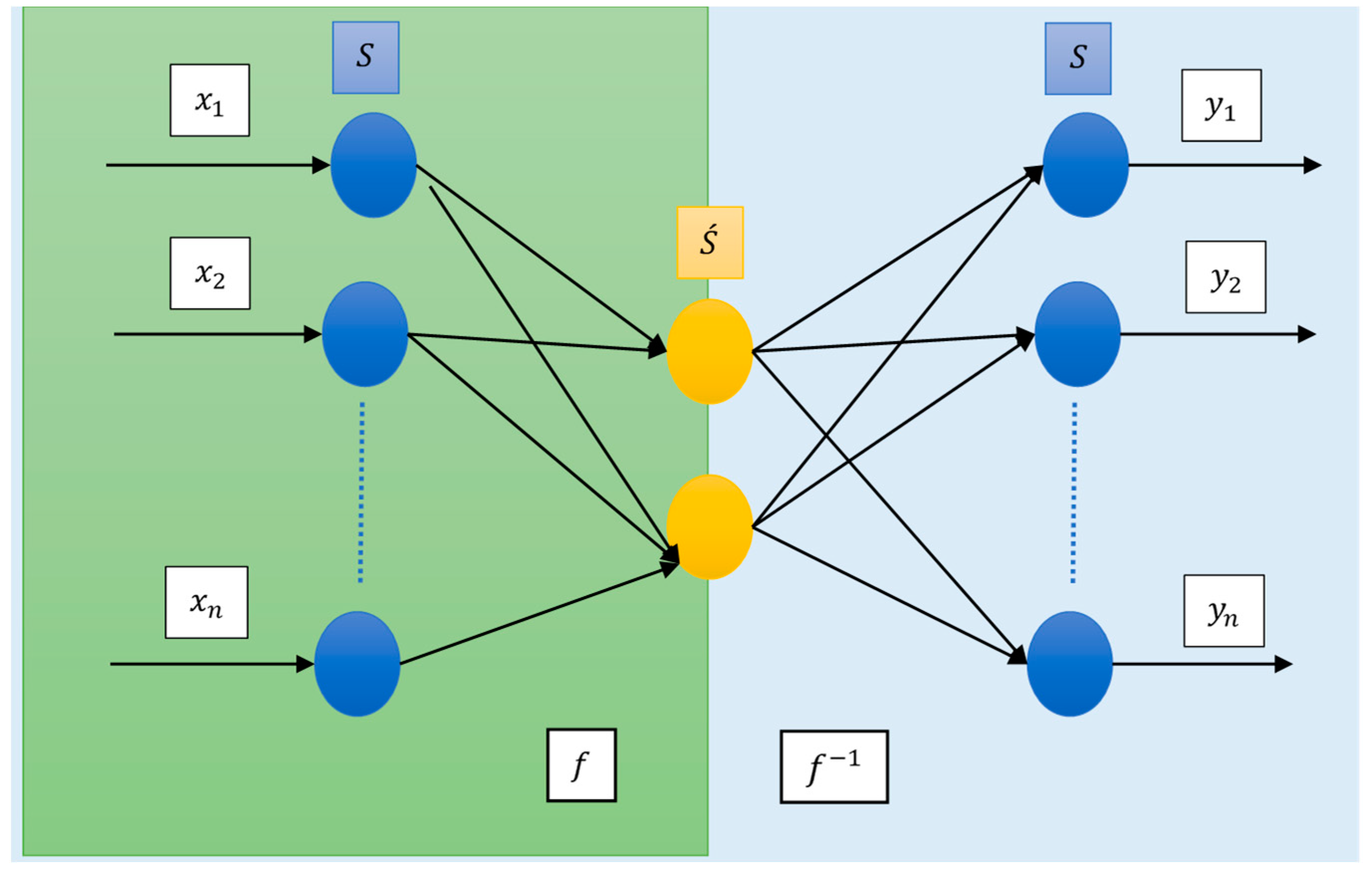
Figure 2.
Structure of proposed stacked autoencoder network.
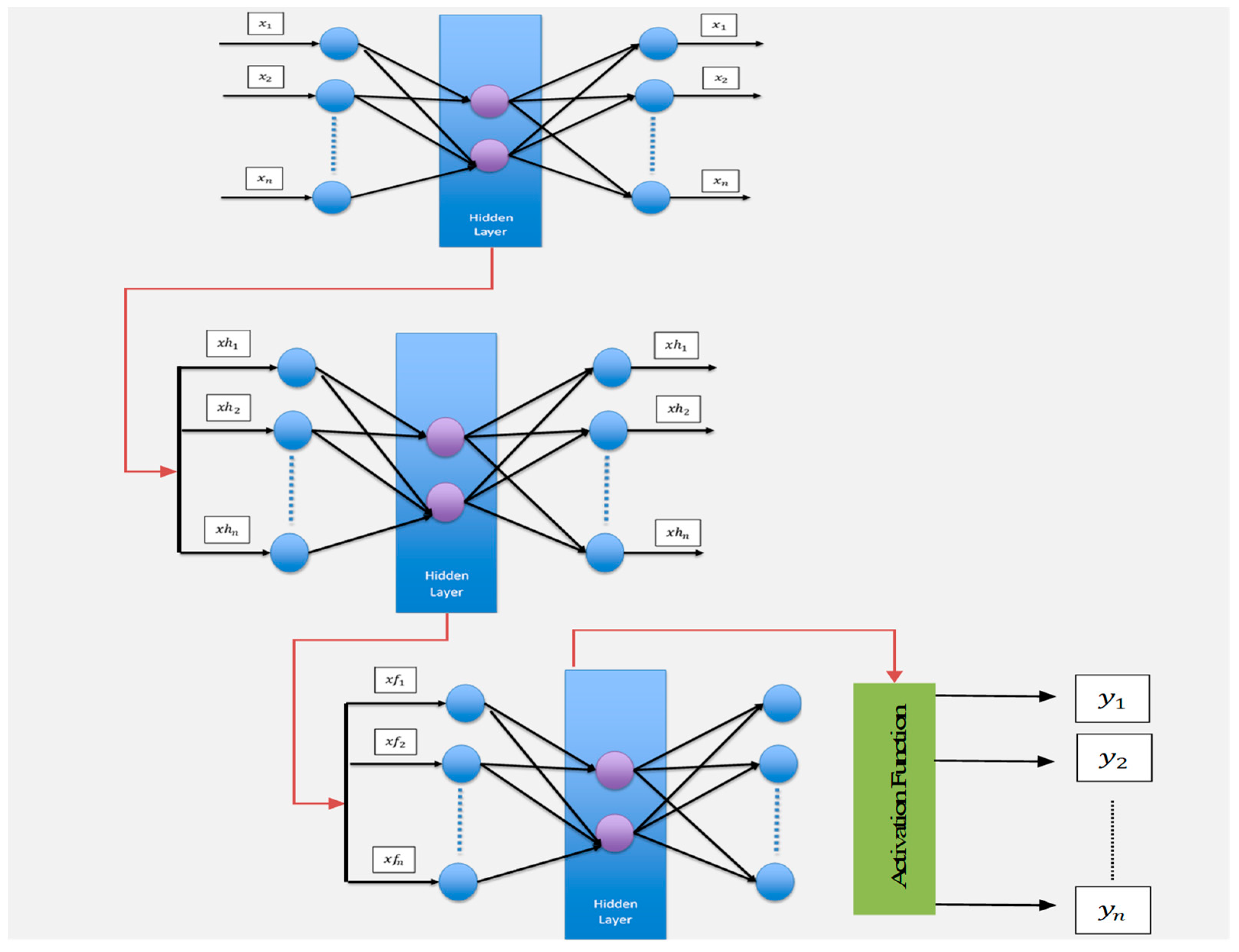
Figure 4.
Structure of 2-layer stacked CNN-BiLSTM-LSTM model.
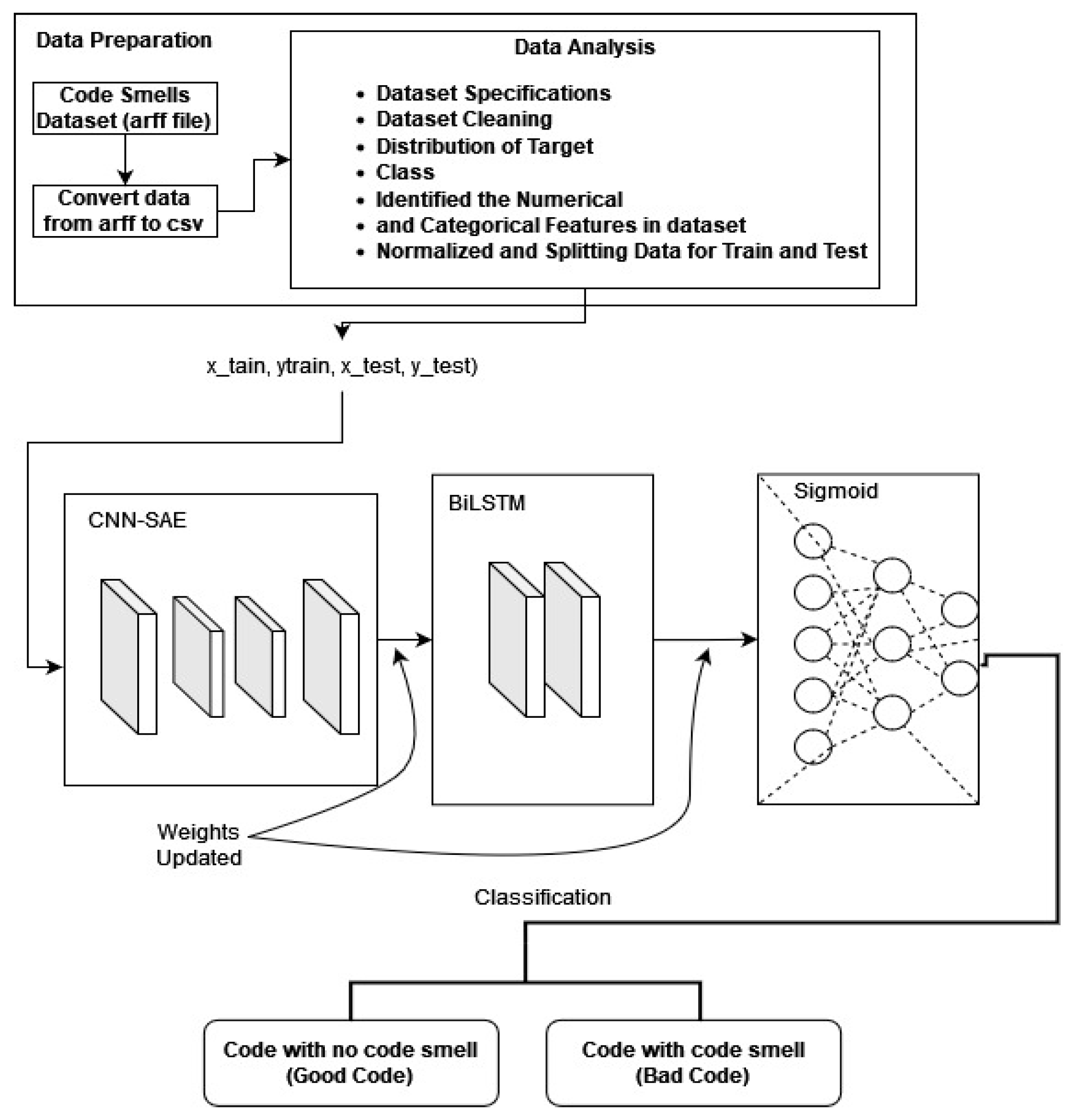
Figure 5.
Data correlation results. (a) God class, (b) Data class, (c) Long method, (d) Feature envy.
Figure 5.
Data correlation results. (a) God class, (b) Data class, (c) Long method, (d) Feature envy.
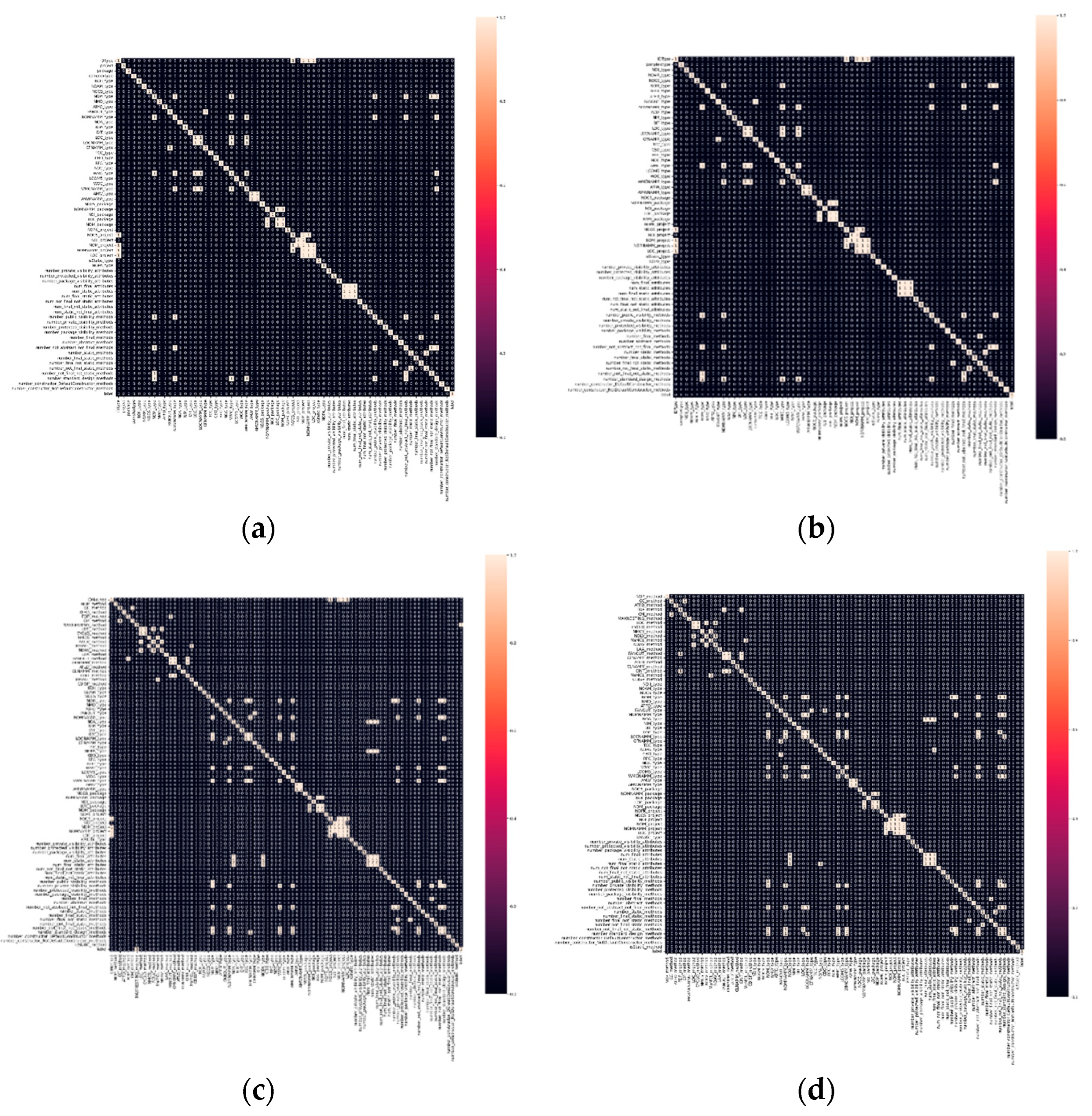
Figure 6.
Training and testing accuracy results for god-class detection using the god-class dataset. (a) CNN model, (b) LSTM model, (c) Proposed model (3-SAE), (d) Proposed model (2-SAE).
Figure 6.
Training and testing accuracy results for god-class detection using the god-class dataset. (a) CNN model, (b) LSTM model, (c) Proposed model (3-SAE), (d) Proposed model (2-SAE).
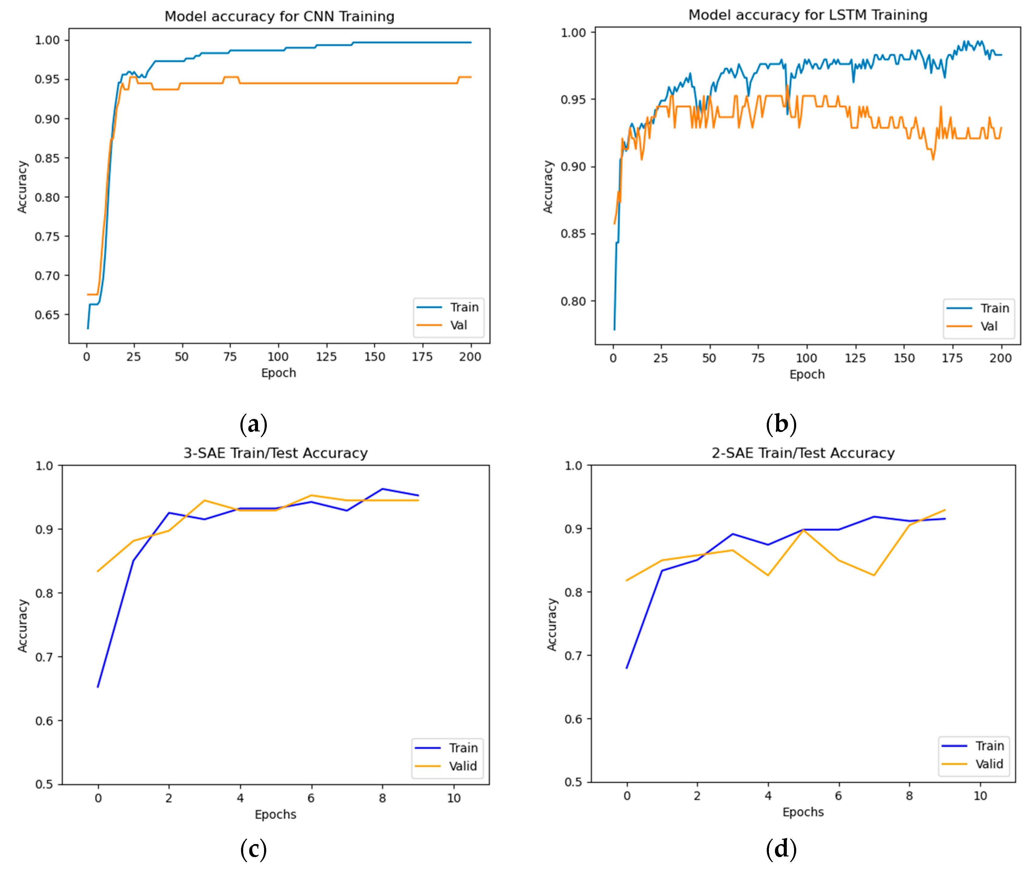
Figure 7.
Training and testing loss results for god-class detection. (a) CNN model, (b) LSTM model, (c) Proposed model (3-SAE), (d) Proposed model (2-SAE).
Figure 7.
Training and testing loss results for god-class detection. (a) CNN model, (b) LSTM model, (c) Proposed model (3-SAE), (d) Proposed model (2-SAE).
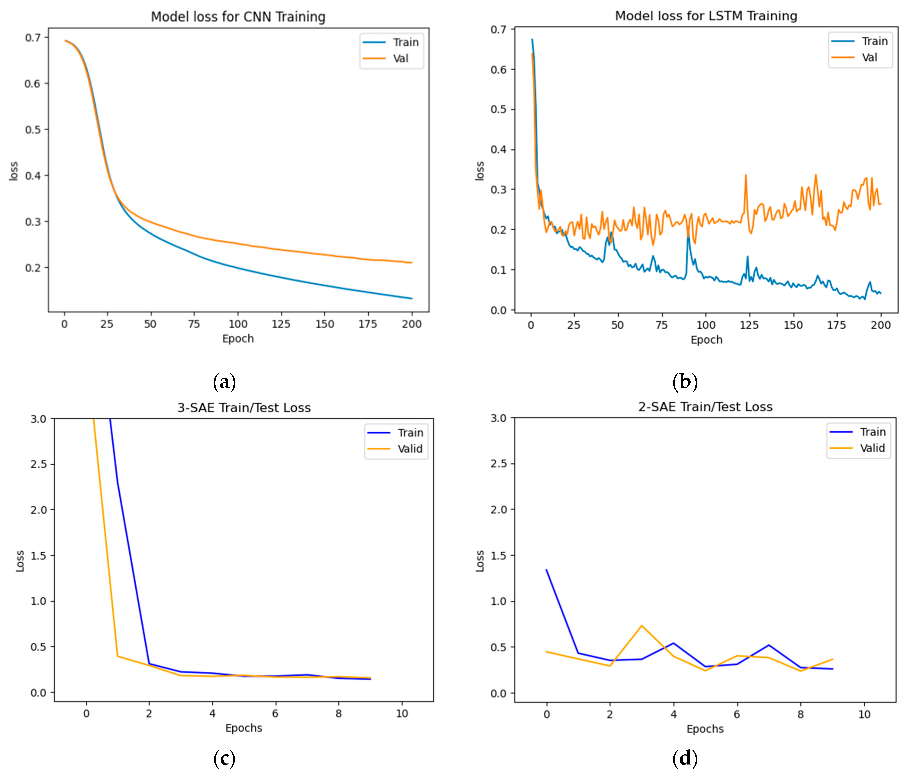
Figure 8.
The accuracy results for data-class dataset detection. (a) CNN model, (b) LSTM model, (c) Proposed model (3-SAE), (d) Proposed model (2-SAE).
Figure 8.
The accuracy results for data-class dataset detection. (a) CNN model, (b) LSTM model, (c) Proposed model (3-SAE), (d) Proposed model (2-SAE).
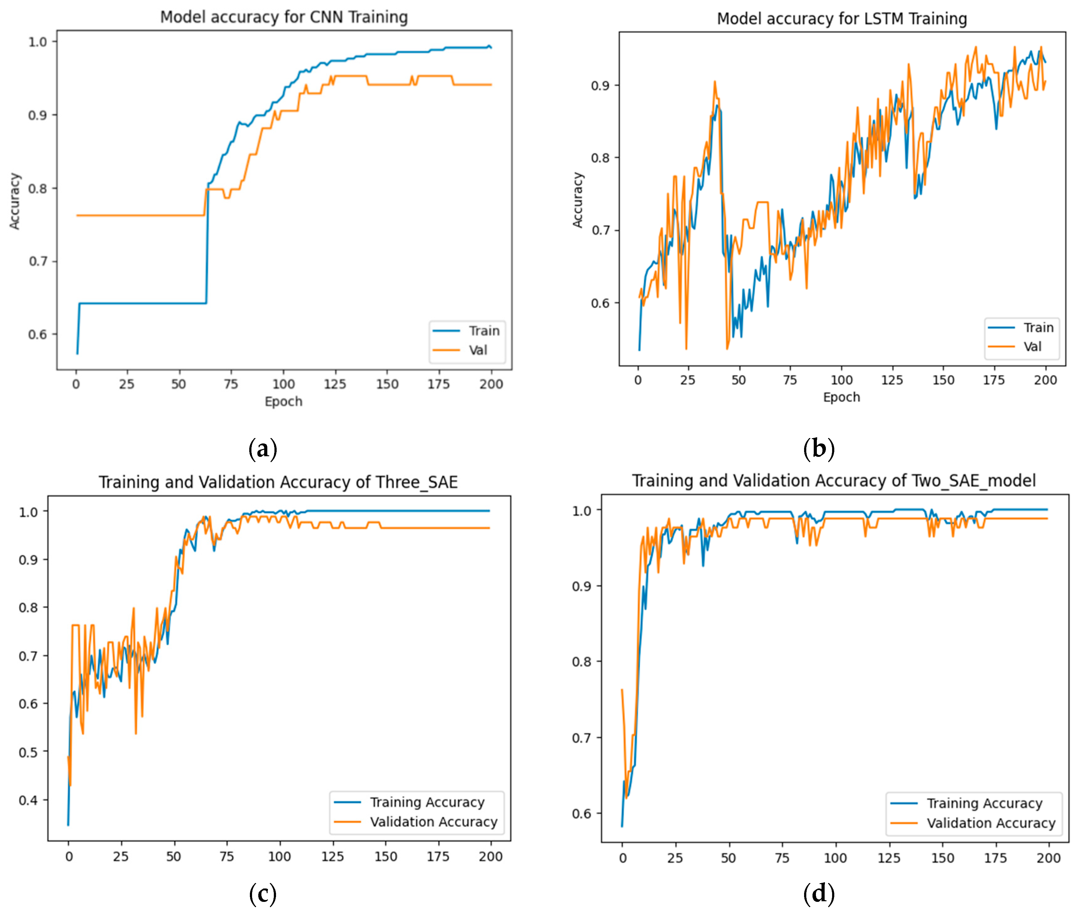
Figure 9.
Training and testing loss results for data-class dataset detection. (a) CNN model, (b) LSTM model, (c) Proposed model (3-SAE), (d) Proposed model (2-SAE).
Figure 9.
Training and testing loss results for data-class dataset detection. (a) CNN model, (b) LSTM model, (c) Proposed model (3-SAE), (d) Proposed model (2-SAE).
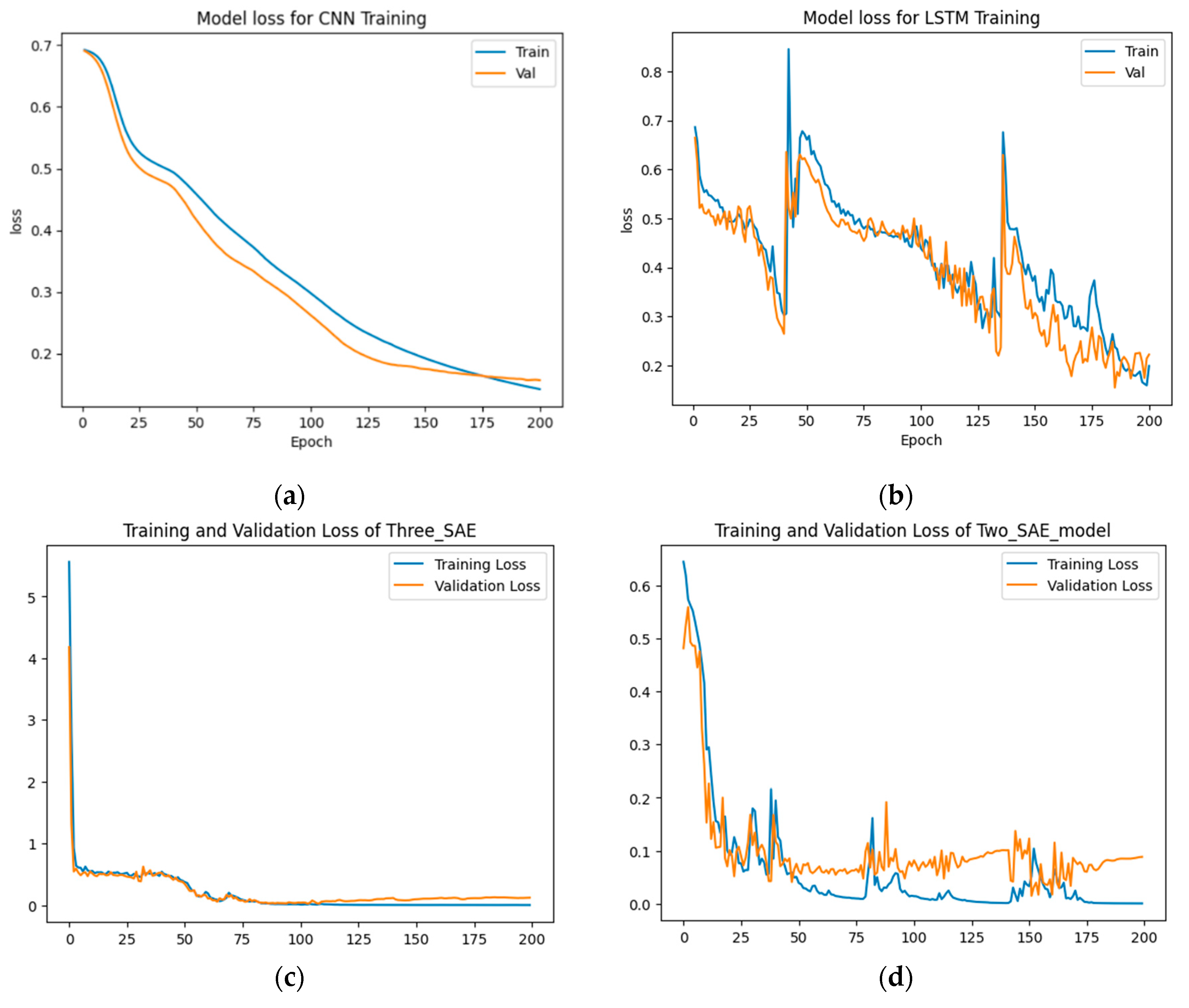
Figure 10.
The accuracy results for long method dataset detection. (a) CNN model, (b) LSTM model, (c) Proposed model (3-SAE), (d) Proposed model (2-SAE).
Figure 10.
The accuracy results for long method dataset detection. (a) CNN model, (b) LSTM model, (c) Proposed model (3-SAE), (d) Proposed model (2-SAE).
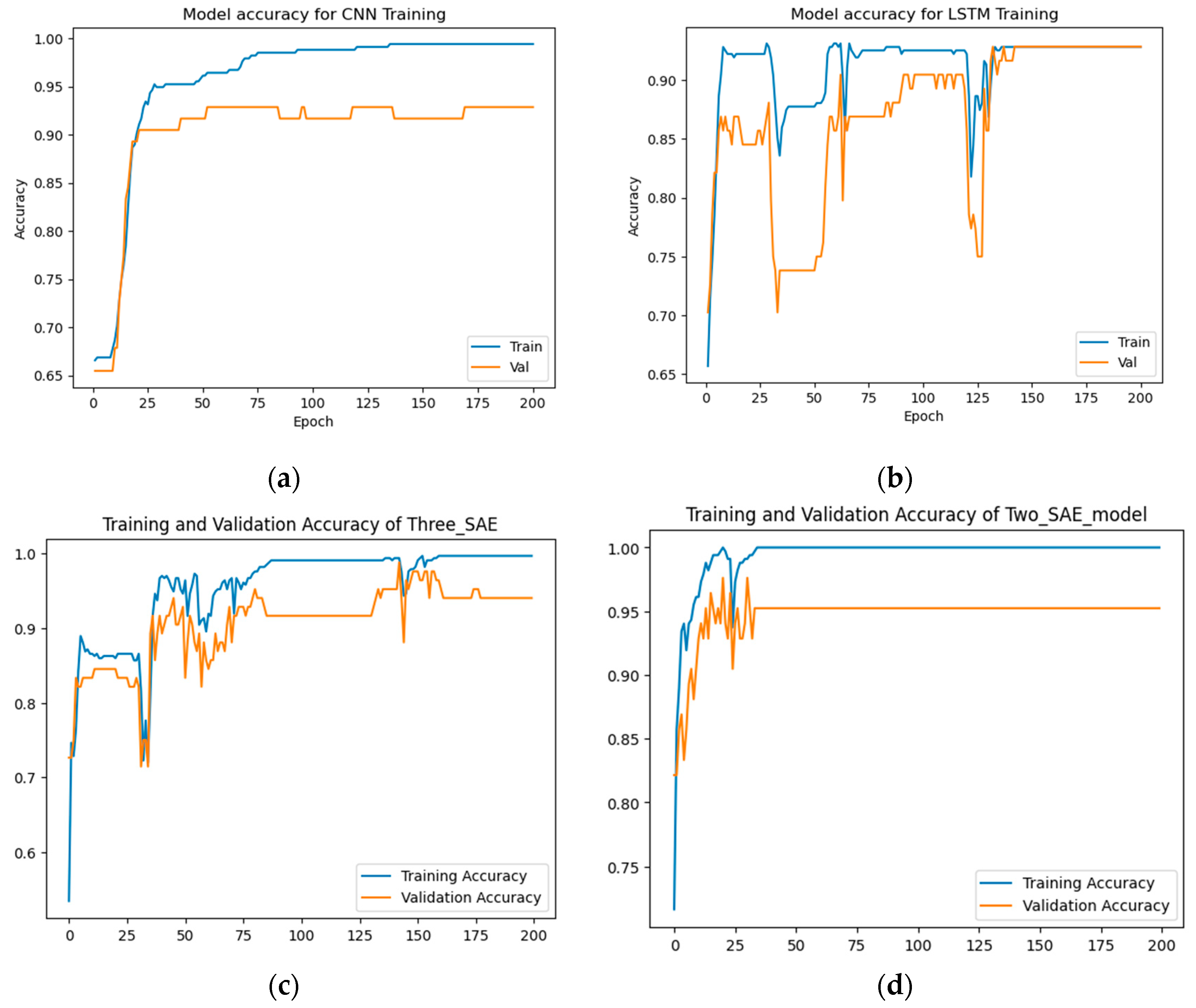
Figure 11.
Training and testing loss results for long method dataset detection. (a) CNN model, (b) LSTM model, (c) Proposed model (3-SAE), (d) Proposed model (2-SAE).
Figure 11.
Training and testing loss results for long method dataset detection. (a) CNN model, (b) LSTM model, (c) Proposed model (3-SAE), (d) Proposed model (2-SAE).
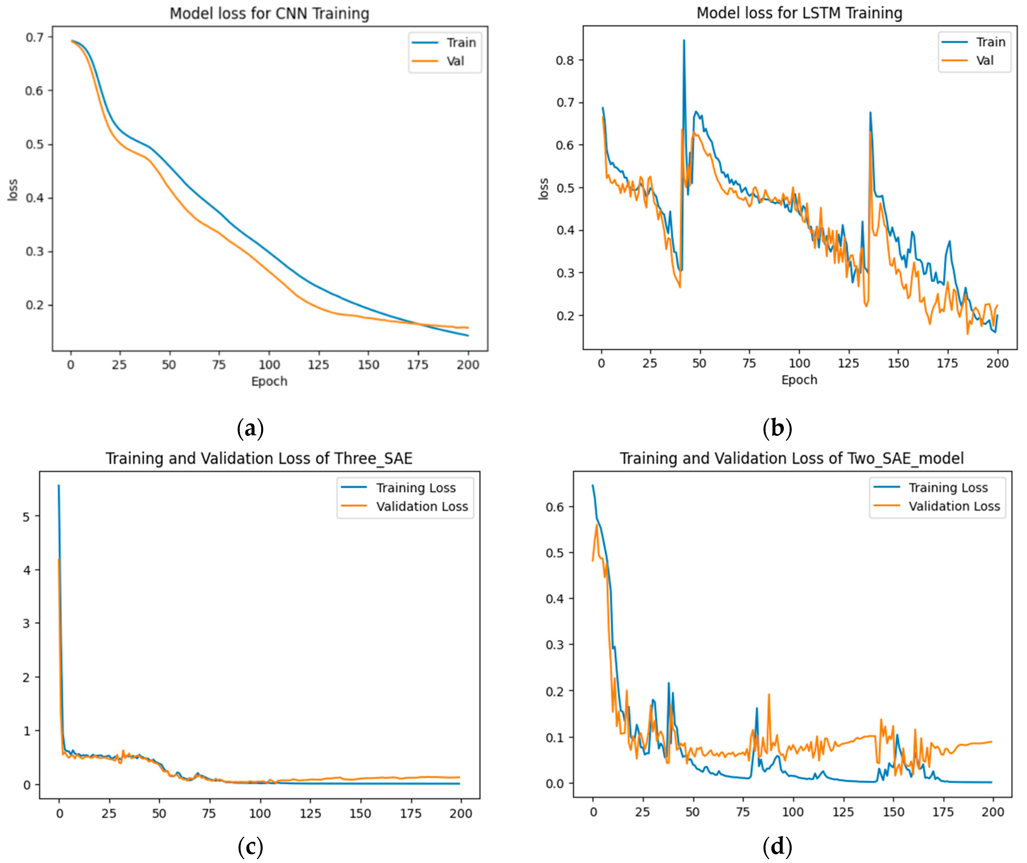
Figure 12.
The accuracy results for feature-envy dataset detection. (a) CNN model, (b) LSTM model, (c) Proposed model (3-SAE), (d) Proposed model (2-SAE).
Figure 12.
The accuracy results for feature-envy dataset detection. (a) CNN model, (b) LSTM model, (c) Proposed model (3-SAE), (d) Proposed model (2-SAE).
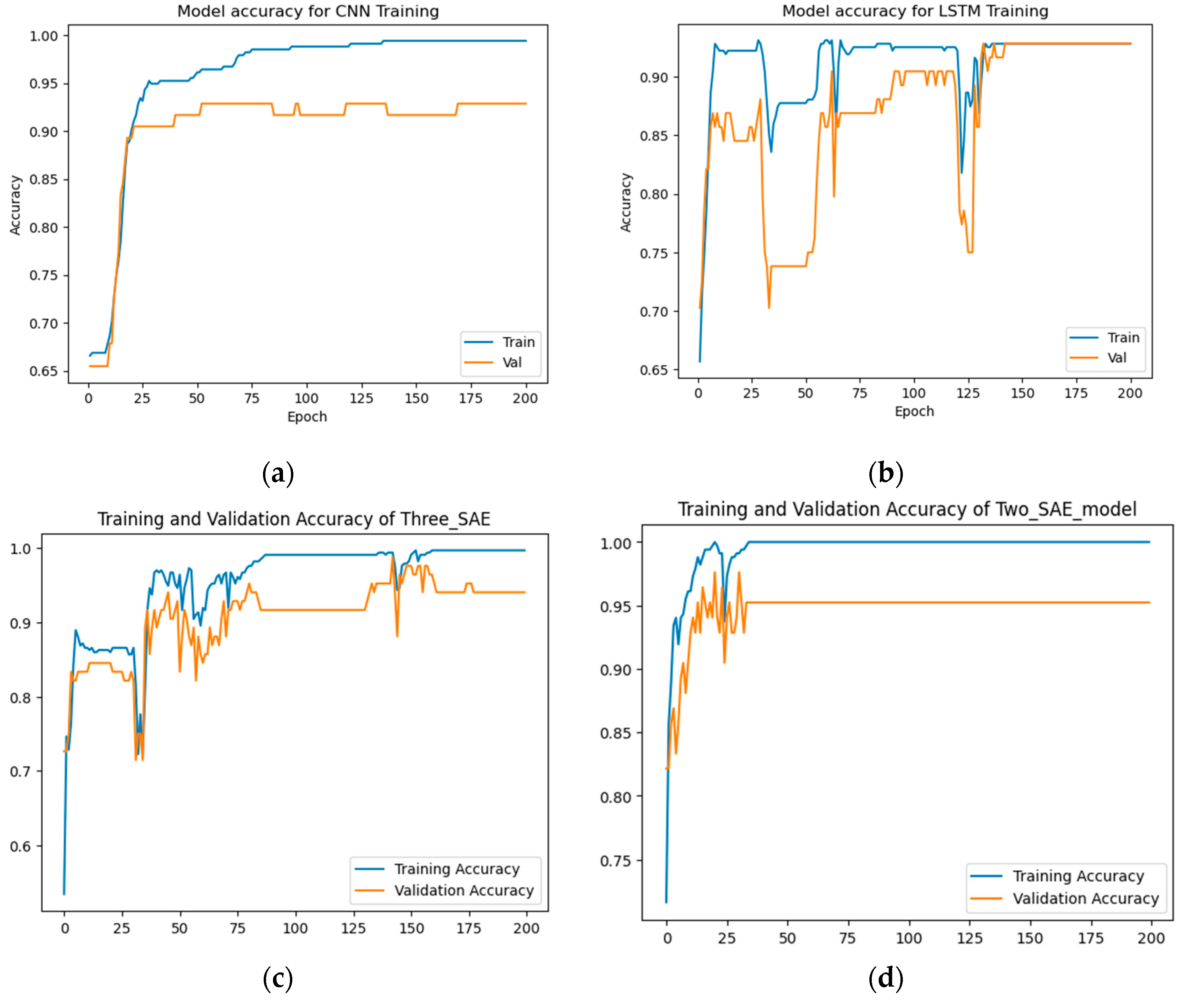
Figure 13.
The training and testing loss results for feature-envy dataset detection. (a) CNN model, (b) LSTM model, (c) Proposed model (3-SAE), (d) Proposed model (2-SAE).
Figure 13.
The training and testing loss results for feature-envy dataset detection. (a) CNN model, (b) LSTM model, (c) Proposed model (3-SAE), (d) Proposed model (2-SAE).
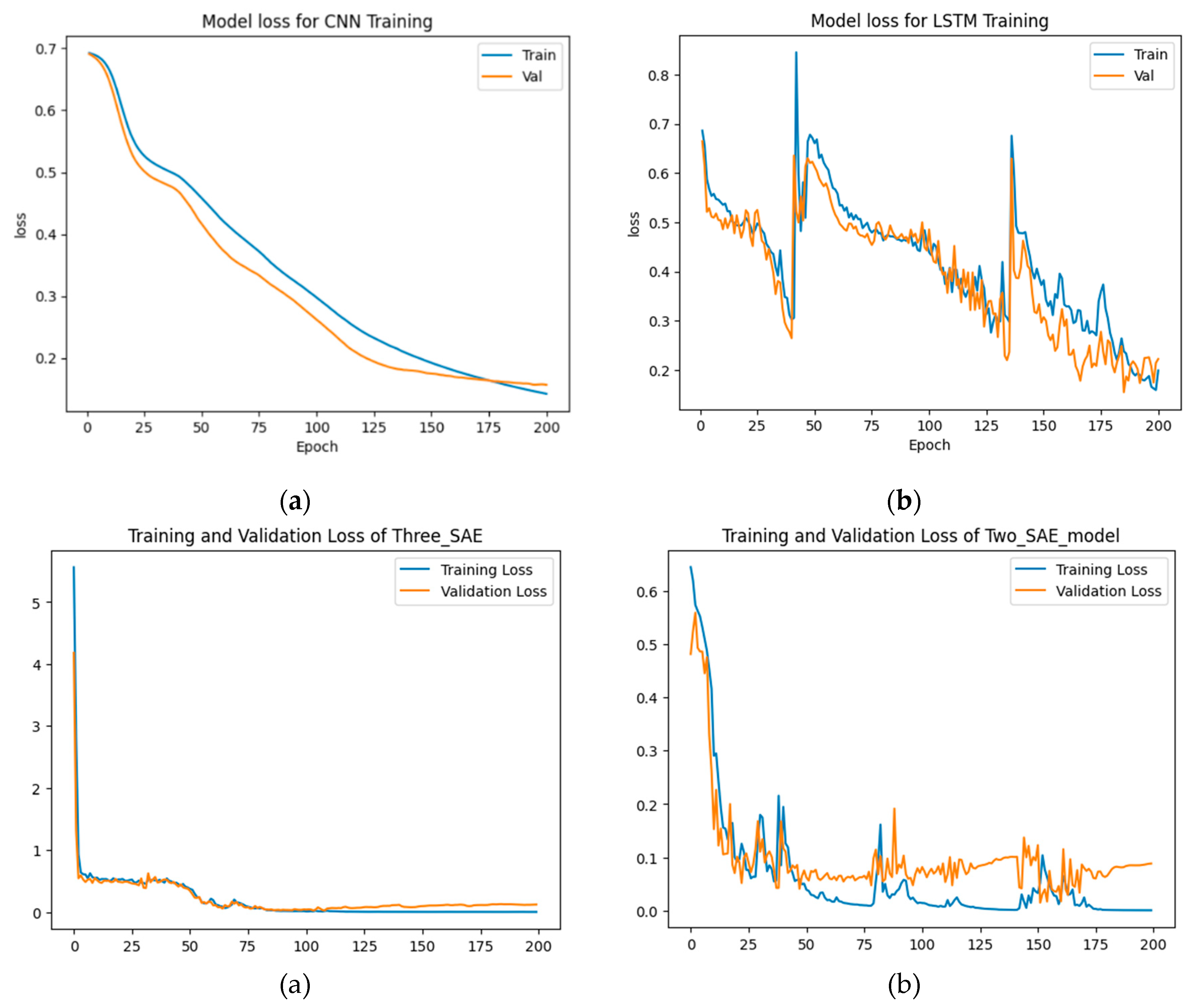

Table 1.
Test Results for Proposed Models and Machine Learning Models.
| Machine Learning Algorithm | Validation Accuracy (%) |
|---|---|
| K-Nearest Neighbor (KNN) | 96.03 |
| Support Vector Machine (SVM) | 93.65 |
| Decision Tree (DT) | 94.44 |
| Stochastic Gradient Descent (SGD) | 94.44 |
| Logistic Regression (LR) | 94.44 |
| eXtreme Gradient Boosting (XGBoost) | 96.83 |
| Proposed Model 1 (3-Layer Stacked Autoencoder) | 97.62 |
| Proposed Model 2 (2-Layer Stacked Autoencoder) | 97.62 |
Table 2.
Results of Tests Using the God Class Dataset for Four Deep Learning Models.
| Metrics | Deep Learning Models | ||||
|---|---|---|---|---|---|
| CNN | LSTM | 3-Layer Stacked Autoencoder | 2-Layer Stacked Autoencoder | ||
| Test Loss | 0.1502 | 0.2635 | 0.1198 | 0.3361 | |
| Test Acc. (%) | 95.24 | 92.86 | 97.62 | 97.62 | |
| Precision (%) | 0 | 0.96 | 0.96 | 0.99 | 0.99 |
| 1 | 0.93 | 0.86 | 0.95 | 0.95 | |
| Recall (%) | 0 | 0.96 | 0.93 | 0.98 | 0.98 |
| 1 | 0.93 | 0.93 | 0.97 | 0.97 | |
| F1-Score (%) | 0 | 0.96 | 0.95 | 0.98 | 0.98 |
| 1 | 0.93 | 0.89 | 0.96 | 0.96 | |
| Training/Testing Time | 19.71 | 106.387 | 265.744 | 27.952 | |
Table 3.
Test Results for Proposed Models and ML Model.
| Machine Learning Algorithm | Validation Accuracy (%) |
|---|---|
| K-Nearest Neighbor (KNN) | 90.48 |
| Support Vector Machine (SVM) | 95.24 |
| Decision Tree (DT) | 97.62 |
| Stochastic Gradient Descent (SGD) | 92.86 |
| Logistic Regression (LR) | 94.05 |
| eXtreme Gradient Boosting (XGBoost) | 97.62 |
| Proposed Model 1 (3-Layer Stacked Autoencoder) | 98.81 |
| Proposed Model 2 (2-Layer Stacked Autoencoder) | 98.81 |
Table 4.
Results of Tests Using the Data Class Dataset for Four DL Models.
| Metrics | Deep Learning Models | ||||
|---|---|---|---|---|---|
| CNN | LSTM | 3-Layer Stacked Autoencoder | 2-Layer Stacked Autoencoder | ||
| Test Loss | 0.2096 | 0.2220 | 0.0539 | 0.0883 | |
| Test Acc. (%) | 95.24 | 90.48 | 98.81 | 98.81 | |
| Precision (%) | 0 | 0.95 | 0.98 | 0.98 | 0.98 |
| 1 | 0.89 | 0.73 | 1.00 | 1.00 | |
| Recall (%) | 0 | 0.97 | 0.89 | 1.00 | 1.00 |
| 1 | 0.85 | 0.95 | 0.95 | 0.95 | |
| F1-Score (%) | 0 | 0.96 | 0.93 | 0.99 | 0.99 |
| 1 | 0.87 | 0.83 | 0.97 | 0.97 | |
| Training/Testing Time | 19.71 | 19.278 | 136.968 | 300.45 | |
Table 5.
Test Results for Proposed Models and ML Models.
| Machine Learning Algorithm | Validation Accuracy (%) |
|---|---|
| K-Nearest Neighbor (KNN) | 90.48 |
| Support Vector Machine (SVM) | 92.86 |
| Decision Tree (DT) | 98.81 |
| Stochastic Gradient Descent (SGD) | 95.24 |
| Logistic Regression (LR) | 95.24 |
| eXtreme Gradient Boosting (XGBoost) | 98.81 |
| Proposed Model 1 (3-Layer Stacked Autoencoder) | 98.81 |
| Proposed Model 2 (2-Layer Stacked Autoencoder) | 98.81 |
Table 6.
Results of Tests Using the Long Method Dataset for Four DL Models.
| Metrics | Deep Learning Models | ||||
|---|---|---|---|---|---|
| CNN | LSTM | 3-Layer Stacked Autoencoder | 2-Layer Stacked Autoencoder | ||
| Test Loss | 0.1903 | 0.2439 | 0.0472 | 0.1091 | |
| Test Acc. (%) | 92.86 | 92.86 | 98.81 | 97.62 | |
| Precision (%) | 0 | 0.95 | 0.98 | 0.98 | 0.98 |
| 1 | 0.89 | 0.73 | 1.00 | 1.00 | |
| Recall (%) | 0 | 0.97 | 0.89 | 1.00 | 1.00 |
| 1 | 0.85 | 0.95 | 0.95 | 0.95 | |
| F1-Score (%) | 0 | 0.96 | 0.93 | 0.99 | 0.99 |
| 1 | 0.87 | 0.83 | 0.97 | 0.97 | |
| Training/Testing Time | 6.200 | 23.81 | 310.45 | 32.3 | |
Table 7.
Test Results for Proposed Models and ML Models.
| Machine Learning Algorithm | Validation Accuracy (%) |
|---|---|
| K-Nearest Neighbor (KNN) | 90.48 |
| Support Vector Machine (SVM) | 92.86 |
| Decision Tree (DT) | 98.81 |
| Stochastic Gradient Descent (SGD) | 95.24 |
| Logistic Regression (LR) | 95.24 |
| eXtreme Gradient Boosting (XGBoost) | 98.81 |
| Proposed Model 1 (3-Layer Stacked Autoencoder) | 98.81 |
| Proposed Model 2 (2-Layer Stacked Autoencoder) | 98.81 |
Table 8.
Results of Tests Using the Feature-Envy Dataset for Four DL Models.
| Metrics | Deep Learning Models | ||||
|---|---|---|---|---|---|
| CNN | LSTM | 3-Layer Stacked Autoencoder | 2-Layer Stacked Autoencoder | ||
| Test Loss | 0.1903 | 0.2439 | 0.0472 | 0.1091 | |
| Test Acc. (%) | 92.86 | 92.86 | 98.81 | 97.62 | |
| Precision (%) | 0 | 0.95 | 0.98 | 0.98 | 0.98 |
| 1 | 0.89 | 0.73 | 1.00 | 1.00 | |
| Recall (%) | 0 | 0.97 | 0.89 | 1.00 | 1.00 |
| 1 | 0.85 | 0.95 | 0.95 | 0.95 | |
| F1-Score (%) | 0 | 0.96 | 0.93 | 0.99 | 0.99 |
| 1 | 0.87 | 0.83 | 0.97 | 0.97 | |
| Training/Testing Time | 6.200 | 23.81 | 310.45 | 32.3 | |
Disclaimer/Publisher’s Note: The statements, opinions and data contained in all publications are solely those of the individual author(s) and contributor(s) and not of MDPI and/or the editor(s). MDPI and/or the editor(s) disclaim responsibility for any injury to people or property resulting from any ideas, methods, instructions or products referred to in the content. |
© 2024 by the authors. Licensee MDPI, Basel, Switzerland. This article is an open access article distributed under the terms and conditions of the Creative Commons Attribution (CC BY) license (http://creativecommons.org/licenses/by/4.0/).
Copyright: This open access article is published under a Creative Commons CC BY 4.0 license, which permit the free download, distribution, and reuse, provided that the author and preprint are cited in any reuse.


