Submitted:
07 March 2024
Posted:
28 March 2024
You are already at the latest version
Abstract
In this paper, two double Jordan-type inequalities are introduced based on the papers [1]-[5]. These inequalities generalize the inequalities obtained in [1]-[5]. As a result, some new upper and lower bounds of the sinc function are obtained. This extension of Jordan’s inequality is enabled by considering the corresponding inequalities through the concept of stratified families of functions elaborated in [6]. Based on this approach, some optimal approximations of the sinc function are derived by determining corresponding minimax approximants, also described in the paper [6].
Keywords:
Jordan’s inequality
; stratified families of functions
; a minimax approximant
; upper and lower bounds of the sinc function
; approximations of the sinc function
1. Introduction
The function:
has numerous applications in mathematics. The basic approximation of the function is given by the well-known Jordan’s inequality:
Theorem 1
Since then, many authors have worked on extensions and improvements of Jordan’s inequality [1,2,3,4,5,8,9,10,11,12,13,14,15,16,17,18,19,20,21,22,23] . In [8], F. Qi, D.-W. Niu and B.-N. Guo did the elaborate research, summarizing previously discovered improvements and applications of Jordan’s inequality, along with related problems. Motivated by some of the following results, this paper provides an additional contribution to this topic.
F. Qi and B.-N. Guo, in the paper [1], provided an enhancement of Jordan’s inequality through the following assertion:
Theorem 2.
Let . Then, it holds:
F. Qi then, in the paper [2], provided further improvement of Jordan’s inequality through the following assertion:
Theorem 3.
Let . Then, it holds:
In the paper [3], K. Deng contributed to improvements of Jordan’s inequality by proving:
Theorem 4.
Let . Then, it holds:
Based on the inequality (3), W. D. Jiang and H. Yun provided further extension of Jordan’s inequality in their paper [4] through the following theorem:
Theorem 5.
Let . Then, it holds:
Shortly afterwards, in the paper [5], J.-L. Li and Y.-L. Li provided a more general statement that encompasses the previous inequalities, (2), (3), (4) and (5), introducing an entire family of inequalities. Namely, the theorem holds:
Theorem 6.
Let . Then, it holds:
Inspired by Theorems 2, 3, 4, 5 and 6, in this paper, based on the concept of stratification of corresponding families of functions from the paper [6], we introduce a new extension of Jordan’s inequality. Namely, by applying stratification, it is possible to extend the inequality (7) so that the parameter n can be a positive real number. The extension of inequalities for real parameters has recently been the subject of various studies [24,25,26,27], see also [28,29,30,31]. Additionally, we provide the best constants for this type of Jordan’s inequality, as well as an analysis of upper and lower bounds and minimax approximations of the function based on the inequalities (2), (3), (4), (5), as well as on the newly obtained inequalities.
2. Preliminaries
Recently, in the paper [6], the authors considered families of functions , where and , which are monotonic with respect to the parameter p. In that paper, such families of functions are referred to as stratified families of functions with respect to the parameter p. If, for each it holds:
then the family of functions is increasingly stratified with respect to the parameter p. If, for each it holds:
then the family of functions is decreasingly stratified with respect to the parameter p.
If it is possible to determine a value of the parameter for which the infimum of the error is attained:
then the function is the minimax approximant of the family of functions on the interval . Based on the stratifiedness, the parameter value is unique.
In this paper, we consider the inequalities (2), (3), (4), (5), (6) and (7) by introducing the corresponding stratified families of functions. When proving inequalities, we will utilize L’Hôpital’s rule for monotonicity, as well as the method for proving MTP (Mixed Trigonometric Polynomial) inequalities described in the paper [32].
L’Hôpital’s rule for monotonicity was described by the author I. Pinelis in the paper [33]. In this paper, we use the following formulation:
Lemma 1
([34]). (Monotone form of L’Hôpital’s rule). Let f and g be continuous functions defined on and differentiable on . Suppose or , and assume that for all . If is an increasing function on , then so is .
The method to prove inequalities of the form on the interval , where is an MTP function, as outlined in [32], is based on determining a downward polynomial approximation with respect to the observed function . In [32], the determination of a polynomial as a polynomial with rational coefficients is considered. If there exists a polynomial such that and on the interval , then holds on the interval . The polynomial is determined as a polynomial with rational coefficients and is examined on the interval with rational endpoints. Then, the proof of the inequality is an algorithmically decidable problem based on Sturm’s theorem, see Theorem 4.2 in [35]. In this paper, the application of Sturm’s theorem will not be necessary for proving polynomial inequalities.
3. Main Results
In this section, several statements are presented and proven, with a special emphasis on the connection between Jordan’s inequality and stratification. Particularly, for each family of functions induced by the aforementioned inequality (7), the best approximations derived from the minimax approximants are identified in Statements Section 3 and Section 3.
Lemma 2.
The two-parameter family of functions:
is individually decreasingly stratified both with respect to the parameter and with respect to the parameter on the interval .
Proof
For the first derivative of with respect to p, it holds:
for and . For the first derivative of with respect to q, it holds:
for and . □
Based on the inequality (7), we introduce the following stratified families of functions in the auxiliary statement:
Lemma 3.
Let:
Then, it holds:
The family of functions:
is decreasingly stratified with respect to the parameter on the interval .
The family of functions:
is increasingly stratified with respect to the parameter on the interval .
Proof
Since , we obtain the one-parameter family of functions:
The first derivative of with respect to q is:
It is evident that:
on the interval for , which concludes the proof.
Since , we obtain the one-parameter family of functions:
The first derivative of with respect to parameter q is:
Let . We now form the function:
Since for , the function is decreasing on the interval . Considering that is a decreasing function and that , we conclude that:
for . Thus, it follows:
on the interval because on . This finishes the proof. □
Statement 1.
Let:
Then, it holds:
If , then the lower bounds of the functio
are given by:
and the constant is the best possible.
If , then the equality:
has a unique solution and it holds:
and
If , then the upper bounds of the function are given by:
and the constant is the best possible.
Each function from the family , for , has exactly one maximum and exactly one minimum at certain points respectively on the interval . Additionally, it holds . The function , for , has exactly one maximum on , and for has exactly one minimum on .
The equality:
has the solution , for the parameter , numerically determined as:
For value:
it holds:
Hence, the minimax approximant of the family of functions is:
which determines the corresponding (minimax) approximation:
Proof
Let us notice that the assertion is equivalent to for and . Based on (10), it holds:
We first prove that the function is monotonic on the interval using L’Hôpital’s rule for monotonicity (Lemma 1). Let us form the functions and on . Note that and . It holds:
We now examine the monotonicity of the function . The first derivative of the function is:
To examine the sign of the function , let us examine the sign of the MTP function:
on the interval .
We prove that using the method from the paper [32]. If we approximate the functions and by Maclaurin polynomials of degrees 4 and 9 respectively, and approximate the function by Maclaurin polynomial of degree 5 in the addend and by Maclaurin polynomial of degree 7 in the addend , then the function has the upward polynomial approximation:
It is evident that on the interval . Thus:
on the observed interval. From here, we conclude that:
on the interval . Thus, is a decreasing function on the interval . Furthermore, since and , based on L’Hôpital’s rule for monotonicity, it follows that is also a decreasing function on the interval .
By applying L’Hôpital’s rule, it can be shown that:
Considering that is a decreasing function on the interval , we conclude that the function , for , does not have a root on the observed interval. Since , we conclude that:
for . Additionally, based on the stratification (Lemma 3), it holds:
for on the interval .
It is easily seen that and . In the part of this proof, it will be shown that each function , for , has exactly one maximum and exactly one minimum on the interval respectively. Hence, the stated inequalities follow.
Continuing from the part of this proof, by multiple applications of L’Hôpital’s rule, it can be shown that:
Considering that is a decreasing function on the interval , we conclude that the function , for , does not have a root on the observed interval. Since , it holds:
for . Additionally, based on the stratification (Lemma 3), it holds:
for on the interval .
Let us examine the monotonicity of functions from the family for on . The fourth derivative of with respect to x is:
where
and
Moreover, the function is defined at both endpoints of the interval , which we will use in the subsequent proof. The first derivative of the function with respect to x is:
for . Therefore, the function is increasing on the interval . Since , it holds that:
on the interval . It is evident that:
for . Hence, we have:
on for . Consequently, each function , for , is increasing on . The third derivative of with respect to x is:
where
It is evident that for . It holds:
Hence, we have:
for . It holds:
Since for , it follows that is an increasing function for . Considering that is an increasing function and that , it can be concluded that:
for . Based on (14), (15) and (16) each function , for , has exactly one minimum on . The second derivative of with respect to x is:
where:
It is evident that for . It holds:
Hence, we have:
for . It holds:
Since for , it follows that is an increasing function for . Considering that is an increasing function and that , it can be concluded that:
for . We have proven that each function , for , has exactly one minimum on . Therefore, based on (17) and (18), for functions , for , there are two possibilities: either they are increasing or they have exactly one maximum and exactly one minimum on respectively. We will prove that:
for , thus, it will be clear that each function , for , has exactly one maximum and exactly one minimum on respectively. The first derivative of with respect to x is:
where:
It holds:
Hence, we have:
for . It is easily seen that:
for . We now examine the sign of the functions , for , at the point . It holds that:
Since for , it follows that is a decreasing function. Considering that is a decreasing function and that , it can be concluded that:
for . Hence, each function , for , has exactly one maximum and exactly one minimum on respectively. Note that is a substitution for the conjunction (20), (21), (22). Additionally, based on the monotonicity of the functions , for , and , we can conclude that each function , for , has exactly one maximum and exactly one minimum on respectively.
By analyzing the monotonicity of the functions , , , and for and for , in a similar manner, it can be concluded that the function , for , has exactly one maximum on , while the function , for , has exactly one minimum on .
Note that the infimum of the error , for , exists and is attained when:
The equation (22) can be numerically solved using the Computer Algebra System Maple, yielding in the value of the parameter being numerically determined as:
which determines the minimax approximant of the family of functions . □
Figure 1 illustrates the stratified family of functions , see (9). Cases for all values of the parameter are shown, with a special emphasis on the cases with constants obtained in Statement 1.
Statement 2.
Let:
Then, it holds:
If , then the upper bounds of the function are given by:
and the constant is the best possible.
If , then the equality:
has a unique solution and it holds:
and
If , then the lower bounds of the function are given by:
and the constant is the best possible.
Each function from the family , for , has exactly one maximum at a point on the interval .
The equality:
has the solution , for the parameter , numerically determined as:
For value:
it holds:
Hence, the minimax approximant of the family of functions is:
which determines the corresponding (minimax) approximation:
Proof
Let us notice that the assertion is equivalent to for . We begin by proving that is monotonic function on the interval for . Through elementary transformations, based on (11), it can be shown that the following equivalence holds:
It is necessary to prove that for every in order for the function to be monotonic on the interval for . We first prove that the function is monotonic on the interval by applying L’Hôpital’s rule for monotonicity. Let us form the functions and on . Note that and . It holds:
We now examine the monotonicity of the function . The first derivative of the function is:
Let us examine the sign of the MTP function:
If we approximate the functions and by Maclaurin polynomials of degrees 6 and 7 respectively, then the function has the downward polynomial approximation:
It is evident that on the interval . Thus:
on the observed interval. From here, we conclude that:
on the observed interval. Thus, is a decreasing function on the interval . Furthermore, since and , based on L’Hôpital’s rule for monotonicity, it follows that is also a decreasing function on the interval . By applying L’Hôpital’s rule, it can be shown that:
Hence, on the interval . Thus, the function , for , is monotonic on the interval . It holds that and . Therefore, is an increasing function and negative on . Considering that , based on the stratification (Lemma 3), it holds:
for on the interval .
Continuing from the previous part of the proof, , by multiple applications of L’Hôpital’s rule, it can be shown that:
The function from (25) determines the values of the parameter q for which the family of functions have extremes or inflection points on the interval . Considering that the function is monotonic on and that and , every function from the family has either exactly one extremum or exactly one inflection point on the interval for , and therefore for , where , since . Let us prove that each function , for , has exactly one maximum on the interval by proving that all these functions are negative in the right neighborhood of zero and positive and increasing in the left neighborhood of .
It holds:
Therefore, there exists a right neighborhood of zero such that:
for . The Taylor expansion of the family of functions around is:
Therefore, there exists a left neighborhood of such that:
for . Based on (26) and (27) the functions , for , have exactly one maximum on the interval and the stated inequalities follow.
The assertion is equivalent to for . Let us notice that for , where . In Statement 1, it has already been proven that for on the interval . Given that the family of functions is increasingly stratified with respect to the parameter q based on Lemma 3, for , it will also hold that:
on the interval .
It has been established in the part of the proof for . Similarly, the proof holds for .
Note that the infimum of the error , for , exists and is attained when:
The equation (27) can be numerically solved using the Computer Algebra System Maple, yielding in the value of the parameter being numerically determined as:
which determines the minimax approximant of the family of functions . □
Figure 2 illustrates the stratified family of functions , see . Cases for all values of the parameter are shown, with a special emphasis on the cases with constants obtained in Statement 2.
In the style of writing Theorem 6, based on Statement 1 and 2, we present the following assertion:
Statement 3.
Let . Then:
For and , it holds:
For and , it holds:
4. Applications
In this section, we present two applications. The first application is about the improvements and expansions of Theorems 2, 3, 4 and 5. The second application refers to obtaining some approximations of the function based on some upper and lower bounds of this function and minimax approximants of the corresponding families of functions.
4.1. Improvements of Theorems 2, 3, 4 and 5
In order to obtain a generalization of all inequalities from Theorems 3, 4, 5 and 6, for the stratified family of functions from Lemma 2, we considered the values of the parameter and as functions depending on the parameter q. It is possible to consider the family of functions from Lemma 2 by fixing either parameter p or q to some real value. For the cases , , and , by applying Statement 1 and 2, improvements and extensions of Theorems 2, 3, 4, 5 respectively can be obtained, as will be shown in the following. Particularly, for each family of functions induced by the considered inequalities, the best approximations derived from the minimax approximants are identified in Statements 4, 5, 6 and 7.
In order to improve and extend Theorem 2, we consider the family of functions for the case . The family of functions reduces to:
and is decreasingly stratified with respect to the parameter on the interval , as proven in Lemma 2. For this family, the following statement holds:
Statement 4.
Let:
Then, it holds:
If , then:
If , then the equality:
has a unique solution and it holds:
and
If , then:
Each function from the family , for , has exactly one maximum at a point on the interval .
The equality:
has the solution , for the parameter , numerically determined as:
For value:
it holds:
Hence, the minimax approximant of the family of functions is:
which determines the corresponding (minimax) approximation:
Proof
The claim follows directly from Statement 1 and based on the stratification. Namely, for , it holds that .
Let us examine the monotonicity of functions for on the interval in a similar manner as in the proof of Statement 1. The second derivative of with respect to x is:
where the function is an MTP function given by:
Let us note that:
on the interval . Thus, the function is decreasing on the observed interval. Considering that is a decreasing function on the interval and that , it follows that:
for . Hence:
for .
The Taylor expansion of the family of functions around zero is:
Therefore, there exists a right neighborhood of zero such that:
for . The Taylor expansion of the family of functions around is:
Therefore, there exists a left neighborhood of such that:
for .
By analyzing the monotonicity of the functions , and for on the interval , in a similar manner as in the proof of Statement 1, based on (32), (33) and (34), it can be concluded that each function , for , has exactly one maximum on the interval . From and , for , the corresponding inequalities follow.
The claim follows directly from Statement 2 and based on the stratification. Namely, for , it holds that .
It has been proven within the proof .
Note that the infimum of the error , for , exists and is attained when:
The equation (35) can be numerically solved using the Computer Algebra System Maple, yielding in the value of the parameter being numerically determined as:
which determines the minimax approximant of the family of functions . □
In order to improve and extend Theorem 3, we consider the family of functions for the case . The family of functions reduces to:
and is decreasingly stratified with respect to the parameter on the interval , as proven in Lemma 2. For this family, the following statement holds:
Statement 5.
Let:
Then, it holds:
If , then:
If , then the equality:
has a unique solution and it holds:
and
If , then:
Each function from the family , for , has exactly one minimum at a point on the interval .
The equality:
has the solution , for the parameter , numerically determined as:
For value:
it holds:
Hence, the minimax approximant of the family of functions is:
which determines the corresponding (minimax) approximation:
Proof
The claim follows directly from Statement 2 and based on the stratification. Namely, for , it holds that .
Let us examine the monotonicity of functions for on the interval in a similar manner as in the proof of Statement 1>. The third derivative of with respect to x is:
where the function is an MTP function given by:
Let us note that:
on the interval . Thus, the function is increasing on the observed interval. Considering that is an increasing function on the interval and that , it follows that:
for . Hence:
for .
The Taylor expansion of the family of functions around zero is:
Therefore, there exists a right neighborhood of zero such that:
for . The Taylor expansion of the family of functions around is:
Therefore, there exists a left neighborhood of such that:
for .
By analyzing the monotonicity of the functions , , and for on the interval , in a similar manner as in the proof of Statement 1, based on (38), (39) and (40), it can be concluded that each function , for , has exactly one minimum on the interval . From and , for , the corresponding inequalities follow.
The claim follows directly from Statement 1 and based on the stratification. Namely, for , it holds that .
It has been proven within the proof .
Note that the infimum of the error , for , exists and is attained when:
The equation (41) can be numerically solved using the Computer Algebra System Maple, yielding in the value of the parameter being numerically determined as:
which determines the minimax approximant of the family of functions . □
In order to improve and extend Theorem 4, we consider the family of functions for the case . The family of functions reduces to:
and is decreasingly stratified with respect to the parameter on the interval , as proven in Lemma 2. For this family, the following statement holds:
Statement 6.
Let:
Then, it holds:
If , then:
If , then the equality:
has a unique solution and it holds:
and
If , then:
Each function from the family , for , has exactly one minimum at a point on the interval .
The equality:
has the solution , for the parameter , numerically determined as:
For value:
it holds:
Hence, the minimax approximant of the family of functions is:
which determines the corresponding (minimax) approximation:
Proof
Analogously to the proof of Statement 5. □
In order to improve and extend Theorem 5, we consider the family of functions for the case . The family of functions reduces to:
and is decreasingly stratified with respect to the parameter on the interval , as proven in Lemma 2. For this family, the following statement holds:
Statement 7.
Let:
Then, it holds:
If , then:
If , then the equality:
has a unique solution and it holds:
and
If , then:
Each function from the family , for , has exactly one minimum at a point on the interval .
The equality:
has the solution , for the parameter , numerically determined as:
For value:
it holds:
Hence, the minimax approximant of the family of functions is:
which determines the corresponding (minimax) approximation:
Proof
Analogously to the proof of Statement 5. □
Figure 3 illustrates the stratified families of functions , , and respectively, see see (30), (36), (42) and (44). For each family, cases for all values of the parameter are shown. Particularly, cases with constants obtained in Statement 4, 5, 6 and 7, some of which are also obtained in Theorems 2, 3, 4 and 5, are singled out.
4.2. Approximations of the Function
In this subsection, we provide some approximations of the function and analyze the maximum approximation errors. The previously obtained upper and lower bounds of the function can be used to derive some approximations of this function. Further, more optimal approximations can be obtained through the corresponding minimax approximants.
In Table 1, we present some upper bounds of the function derived from Theorems 2, 3, 4 and 5, that is, Statements Section 4.1, Section 4.1, Section 4.1 and Section 4.1 and Statements Section 3 and Section 3. It is noteworthy that the upper bound from Theorem 3 (the best upper bound from Statement Section 4.1) is identical to the best upper bound from Statement Section 3.
In Table 2, we present some lower bounds of the function derived from Theorems 2, 3, 4 and 5, that is, Statements 4, 5, 6 and 7 and Statements 1 and 2. It is noteworthy that the best lower bound from Statement Section 3 is identical to the best lower bound from Statement Section 3.
In Table 3, we present some minimax approximations of the function derived from the minimax approximants of the families , , , , and respectively. These families are considered in Statements 4, 5, 6 and 7 with the aim of improving Theorems 2, 3, 4 and 5, respectively, and in Statements 1 and 2.
5. Conclusion
In this paper, two double Jordan-type inequalities have been derived, encompassing the inequalities obtained in the papers [1,2,3,4,5]. These inequalities were explored in the context of stratified families of functions, a concept introduced in recent research [6]. The introduction of stratified families of functions enables the derivation of known results for specific parameter choices, including the analysis of parameter values previously unknown in the Theory of Analytic Inequalities. Furthermore, we identify parameter values within each examined family of functions for which the function, as a member of that family, exhibits some optimal properties (minimax approximant). Based on these minimax approximants and functions representing the upper and lower bounds of the function, we provided some approximations of the function. Additionally, we analyzed the errors associated with all mentioned approximations.
It is crucial to emphasize that the minimax approximant of the stratified family of functions is the function for which the minimal error in approximations is obtained within the given family of functions. Therefore, identifying those parameter values is significant Approximation Theory.
By considering the stratified family of functions individually with respect to two parameters, we were able to analyze Jordan-type inequalities in a unified manner, resulting in both previously established and novel findings. Future research endeavors will focus on extending this approach even further.
Author Contributions
The authors contributed equally to this work.
Funding
This research received no external funding.
Data Availability Statement
Not applicable.
Acknowledgments
The authors are supported by the Serbian Ministry of Education, Science and Technological Development, under project 451-03-47/2023-01/200103.
Conflicts of Interest
The authors declare no conflict of interest.
Abbreviations
The following abbreviations are used in this manuscript:
| MTP | Mixed Trigonometric Polynomial |
References
- Qi, F.; Guo, B.-N. On generalizations of Jordan’s inequality (in Chinese). Coal Higher Education, supplement, 1993; 32–33. [Google Scholar]
- Qi, F. Extensions and sharpenings of Jordan’s and Kober’s inequality (in Chinese). Journal of Mathematics for Technology, 1996; 12, 98–101. [Google Scholar]
- Deng, K. The noted Jordan’s inequality and its extensions (in Chinese). Journal of Xiangtan Mining Institute, 1995; 10, 60–63. [Google Scholar]
- Jiang, W. D.; Yun, H. Sharpening of Jordan’s inequality and its applications. Journal of Inequalities in Pure and Applied Mathematics, 2006; 7, 1–4. [Google Scholar]
- Li, J.-L.; Li, Y.-L. On the Strengthened Jordan’s Inequality. Journal of Inequalities and Applications 2008, 2007, 1–8. [Google Scholar] [CrossRef]
- Malešević, B.; Mihailović, B. A minimax approximant in the theory of analytic inequalities. Applicable Analysis and Discrete Mathematics, 2021; 15, 486–509. [Google Scholar]
- Mitrinović, D. Analytic Inequalities; Publisher: Springler-Verlag Berlin, Germany, 1970. [Google Scholar]
- Qi, F.; Niu, D.-W. Refinements, Generalizations, and Applications of Jordan’s Inequality and Related Problems. Journal of Inequalities and Applications 2009, 2009, 1–52. [Google Scholar] [CrossRef]
- Özban, A. Y. A new refined form of Jordan’s inequality and its applications. Applied Mathematics Letters 2006, 19, 155–160. [Google Scholar] [CrossRef]
- Li, J.-L. An identity related to Jordan’s inequality. International Journal of Mathematics and Mathematical Sciences 2006, 2006, 1–6. [Google Scholar] [CrossRef]
- Zhu, L. Sharpening Jordan’s inequality and the Yang Le inequality. Applied Mathematics Letters 2006, 19, 240–243. [Google Scholar] [CrossRef]
- Zhu, L. Sharpening Jordan’s inequality and the Yang Le inequality, II. Applied Mathematics Letters 2006, 19, 990–994. [Google Scholar] [CrossRef]
- Zhu, L. A general refinement of Jordan-type inequality. Computers & Mathematics with Applications 2008, 55, 2498–2505. [Google Scholar]
- Niu, D.-W.; Huo, Z.-H.; Cao, J.; Qi, F. A general refinement of Jordan’s inequality and a refinement of L. Yang’s inequality. Integral Transforms and Special Functions, 2008; 19, 157–164. [Google Scholar]
- Chen, C.-P.; Debnath, L. Sharpness and generalization of Jordan’s inequality and its application. Applied Mathematics Letters 2012, 25, 594–599. [Google Scholar] [CrossRef]
- Barbu, C.; Pişcoran, L.-I. Jordan type inequalities using monotony of functions. Journal of Mathematical Inequalities, 2014; 8, 83–89. [Google Scholar]
- Aharonov, D.; Elias, U. More Jordan type inequalities. Mathematical Inequalities & Applications; 2014; Volume 17, pp. 1563–1577. [Google Scholar]
- Alzer, H.; Kwong, M. K. On Jordan’s inequality. Periodica Mathematica Hungarica 2018, 77, 191–200. [Google Scholar] [CrossRef]
- Zhang, L.; Ma, X. New Refinements and Improvements of Jordan’s Inequality. Mathematics, 2018; 2018, 1–8. [Google Scholar]
- Zhang, L.; Ma, X. New Polynomial Bounds for Jordan’s and Kober’s Inequalities Based on the Interpolation and Approximation Method. Mathematics, 2019; 7, 1–9. [Google Scholar]
- Zhang, B.; Chen, C.-P. Sharpness and generalization of Jordan, Becker-Stark and Papenfuss inequalities with an application. Journal of Mathematical Inequalities, 2019; 13, 1209–1234. [Google Scholar]
- Haque, N. A Short Calculus Proof of Jordan’s Inequality. Cambridge Open Engage (Preprint) 2020, 1–1. [Google Scholar]
- Popa, E. C. A note on Jordan’s inequality. General Mathematics, 2020; 28, 97–102. [Google Scholar]
- Malešević, B.; Mićović, M. Exponential Polynomials and Stratification in the Theory of Analytic Inequalities. Journal of Science and Arts, 2023; 23, 659–670. [Google Scholar]
- Malešević, B.; Jovanović, D. Frame’s Types of Inequalities and Stratification. CUBO, A Mathematical Journal, 2024; 26, 1–15. [Google Scholar]
- Chen, S.; Ge, X. A solution to an open problem for Wilker-type inequalities. Journal of Mathematical Inequalities, 2021; 15, 59–65. [Google Scholar]
- Malešević, B.; Mihailović, B.; Nenezić Jović, M.; Milinković, L. Some minimax approximants of D’Aurizio trigonometric inequalities. HAL (Preprint) 2022, 1–9. [Google Scholar]
- Chen, C.-P.; Mortici, C. The relationship between Huygens’ and Wilker’s inequalities and further remarks. Applicable Analysis and Discrete Mathematics, 2023; 17, 92–100. [Google Scholar]
- Sándor, J. On D’Aurizio’s trigonometric inequality. Journal of Mathematical Inequalities, 2016; 10, 885–888. [Google Scholar]
- Sándor, J. Extensions of D’Aurizio’s trigonometric inequality. Notes on Number Theory and Discrete Mathematics, 2017; 23, 81–83. [Google Scholar]
- Hung, L.-C.; Li, P.-Y. On generalization of D’Aurizio-Sándor inequalities involving a parameter. Journal of Mathematical Inequalities, 2018; 12, 853–860. [Google Scholar]
- Malešević, B.; Makragić, M. A method for proving some inequalities on mixed trigonometric polynomial functions. Journal of Mathematical Inequalities, 2016; 10, 849–876. [Google Scholar]
- Pinelis, I. L’Hospital type rules for monotonicity, with applications. Journal of Inequalities in Pure and Applied Mathematics, 2002; 3, 1–5. [Google Scholar]
- Estrada, R.; Pavlović, M. L’Hôpital’s monotone rule, Gromov’s theorem, and operations that preserve the monotonicity of quotients. Publications de l’Institut Mathematique, 2017; 101, 11–24. [Google Scholar]
- Cutland, N. Computalibity: an introduction to recursive funtion theory; Publisher: Cambridge University Press, Great Britain, 1980. [Google Scholar]
Figure 1.
Stratified family of functions , see .
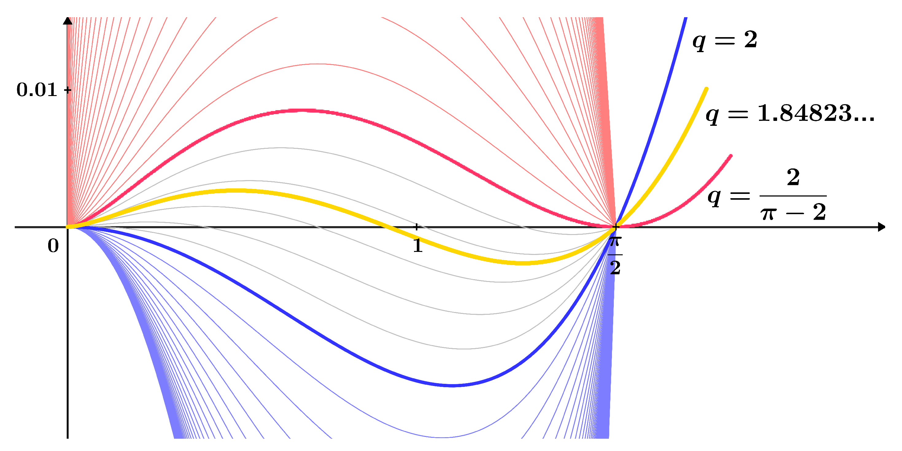
Figure 2.
Stratified family of functions , see .
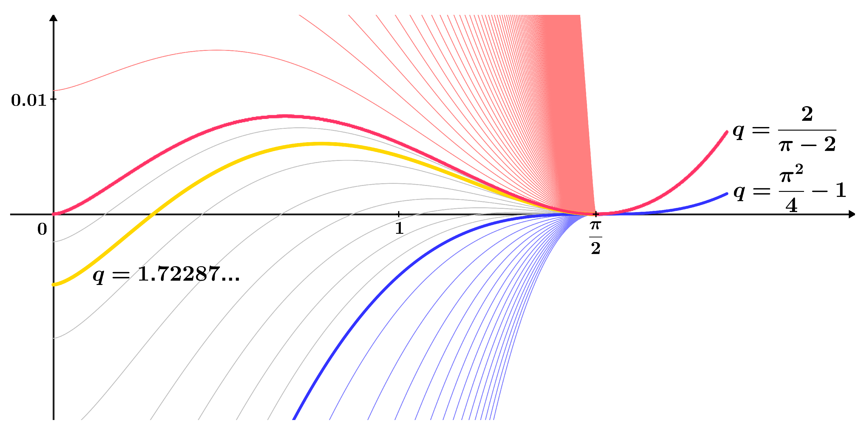
Figure 3.
Stratified families of functions: (a) , (b) , (c) , (d) .
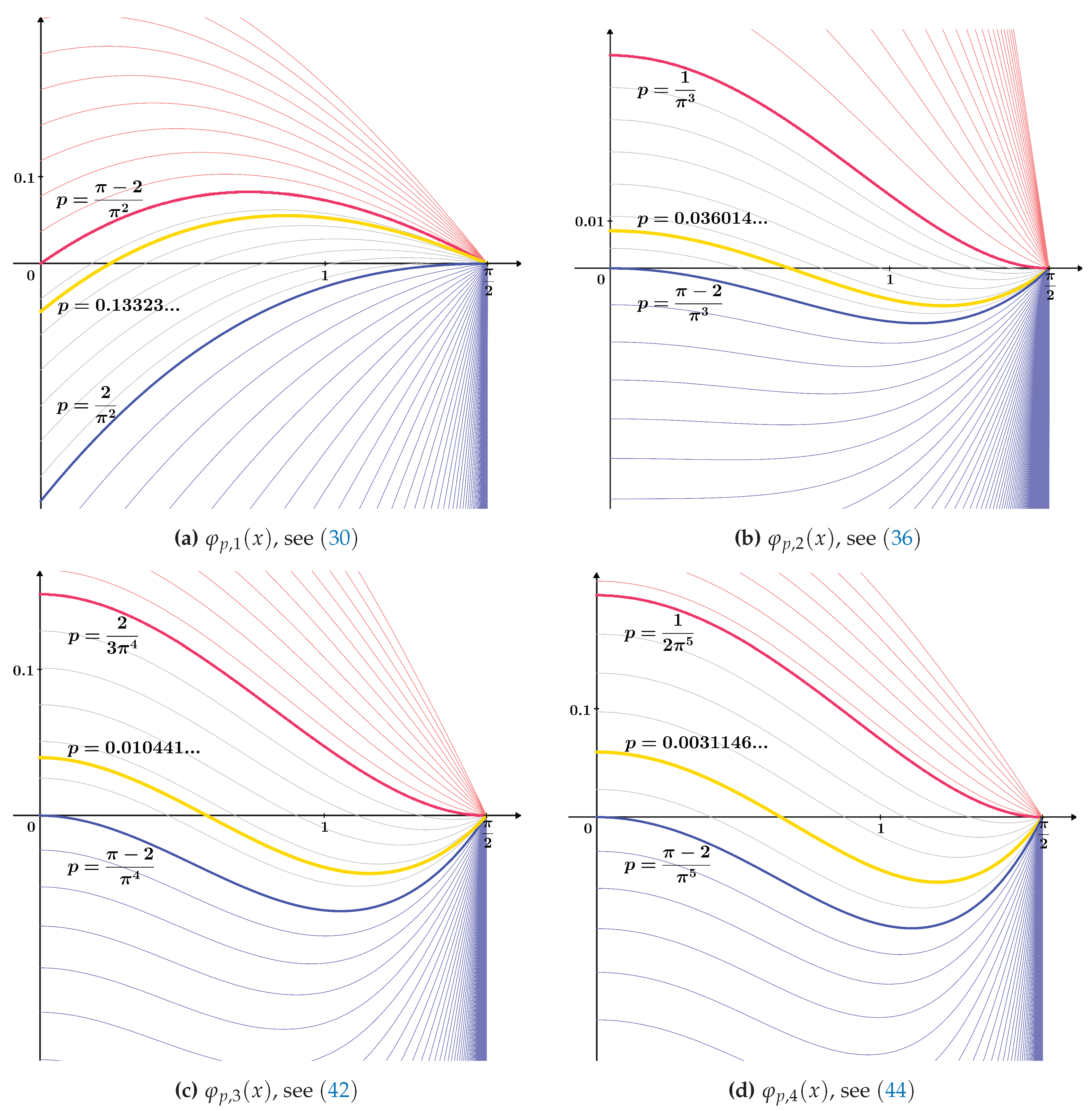

Table 1.
Upper bounds of the function
| Maximum deviation | |
|---|---|
| Upper bound of the function | from the function |
| over the interval | |
Table 2.
Lower bounds of the function.
| Maximum deviation | |
|---|---|
| Lower bound of the function | from the function |
| over the interval | |
Table 3.
Minimax approximations of the function
| Maximum deviation | |
|---|---|
| Minimax approximation of the function | from the function |
| over the interval | |
Disclaimer/Publisher’s Note: The statements, opinions and data contained in all publications are solely those of the individual author(s) and contributor(s) and not of MDPI and/or the editor(s). MDPI and/or the editor(s) disclaim responsibility for any injury to people or property resulting from any ideas, methods, instructions or products referred to in the content. |
© 2024 by the authors. Licensee MDPI, Basel, Switzerland. This article is an open access article distributed under the terms and conditions of the Creative Commons Attribution (CC BY) license (http://creativecommons.org/licenses/by/4.0/).
Copyright: This open access article is published under a Creative Commons CC BY 4.0 license, which permit the free download, distribution, and reuse, provided that the author and preprint are cited in any reuse.


