Submitted:
26 March 2024
Posted:
26 March 2024
Read the latest preprint version here
Abstract
A testable hypothesis with quantitative predictions is put forward, proposing that strong acids produced on land are a major cause of increasing atmospheric pCO2. Our modelling analysis of reactions by dissolved inorganic carbon shows that increasing atmospheric CO2 could be caused thermodynamically by falling land surface pH values. This hypothesis challenges the imbalance assumed between the global uptake of CO2 by photosynthesis and emissions of CO2 from all sources, including the combustion of fossil fuels. Strong acids generated by oxygen from reduced nitrogen and sulphur emits CO2 almost stoichiometrically from dissolved bicarbonate in the pH range of most global soils from pH 6.5 to above 8. Each general decrease of aqueous pH value of 0.01 units from acidification of surface water potentially increases the pCO2 in the atmosphere by about 7 ppmv. Contrary to prevailing assumptions that CO2 emissions from combusting fossil fuels can remain in the atmosphere for more than a millennium, such emissions may be partly nullified by global greening from enhanced rates of photosynthesis as well as oceanic absorption. The surface pH value of the ocean has been shown to decrease as atmospheric pCO2 rises. Therefore, our qualitative estimates of increasing atmospheric CO2 driven by irreversible acidification on land are critical and need broad scale validation. To the extent that significant acidification of the land is occurring, through export of alkaline produce, the use of artificial nitrogen fertilisation and possible other causes, the prevailing methods of reducing CO2 emissions will fail. However, these acidifying processes on land have not been considered by previous biogeochemical reviews. Despite counter measures, including carbon capture and geological storage, the increasing Keeling curve for pCO2 may continue to rise because zero carbon policies do not address such a major cause. This hypothesis can be tested by in situ experiments in neutral soils and water, designed to compare CO2 emissions under the acidifying conditions described in this article with those when corrective counter measures are applied.
Keywords:
CO2 emissions
; climate change
; soil pH
; alkalinity of plant produce
; export from rural to urban environments
; bicarbonate and carbonate
; limestone as soil ameliorant
; Keeling curve
1. Introduction
Our recent article [1] tested one physico-chemical hypothesis that seasonal variation in seawater temperature was a probable cause of changing atmospheric pCO2. That Thermal model linked seasonal variations in the temperature of the ocean’s surface layer as causing differences in the relative thermodynamic fugacity of CO2 in surface seawater [1] and in air, also affecting the solubility of calcite. Particularly in the northern hemisphere oceans, calcite precipitation in surface water in summer must lower pH, increasing seawater CO2 fugacity (fCO2) as atmospheric pCO2 becomes lowest, promoting CO2 transfer to air as winter progresses, a process reversing later as calcite redissolves in cooling seawater, raising pH values and equilibrating with higher CO2 to the atmosphere in early spring. Non-equilibrium transport processes at the interface between air and the surface of the ocean explain [1] most of the seasonal oscillation in pCO2 (Figure 1), even up to 15 ppmv observed by Keeling [2] at Point Barrow in the Arctic. Therefore the pCO2 oscillation is not a result of regional seasonal imbalances in photosynthesis and respiration. Van’t Hoff analyses of the variation of equilibrium constants with temperature showed [1] that the enthalpy of formation of bicarbonate and carbonate was endothermic, favoured by summer warming consistent with Le Chatelier’s principle. An increase in mixing layer carbonate (CO32-) in summer warming precipitates calcite (CaCO3) and lowers pH providing conditions favouring higher fugacity for CO2 in seawater CO2 and its transfer to air. This seasonal oscillation in pCO2 on Mauna Loa is shown in the subset of Figure 1. We estimated [1] that about 30 Gtonnes of CO2 is now exchanged annually between the sea mixing layer and the atmosphere, particularly in the northern hemisphere, on a seasonal basis. The CO2 transfer is similar in magnitude to the total annual emission of fossil fuels, some 5% of the total CO2 emissions from all sources.
Our numerical computation [1] predicted that the range of thermal fluctuations in the northern hemisphere could reversibly favour absorption from air of more than one mole of CO2 per square metre in summer with calcite formation potentially augmenting shallow limestone reefs, despite falling pH, if there is a trend for increasing seawater temperature. Standard enthalpy analysis of key reactions indicated why this oscillation is more obvious in the northern hemisphere. Here seasonal variations in water temperature (ca. 7.1 oC) are almost twice those in the southern hemisphere (ca. 4.7 oC) with a greater depth of the surface mixing zone of seawater in the southern oceans. It was concluded that the relative significance of terrestrial biotic and seawater abiotic processes in seawater on the seasonal oscillation in the atmosphere can only be assessed by direct seasonal measurements in seawater.
Against this background research that established a firm role for temperature in regulating seasonal flows between the ocean and the atmosphere we were confident we could also investigate the role of another control of the DIC system normally observed in the laboratory. To what extent did the pH value of the land surface influence the flows of CO2 at the boundary layer? The high sensitivity of equilibrium pCO2 to changes in pH value in seawater suggested that similar controls might occur with land waters and with moist soil. In the rest of this article we intend to show that this is also a significant control factor.
1.1. Background Inorganic Chemistry and Responses to Changing Water pH Values
This article tests a second physico-chemical hypothesis regarding the Keeling curve, proposing that decreasing land surface pH values cause a long-term planetary trend for increasing atmospheric pCO2. Our article will first investigate whether there are likely anthropogenic reasons for such a trend, the environmental production of strong acid (H+) causing the following Reactions (1) and (2). The equilibrium constants are shown inversely to those for reversed reactions of those given in our previous article [1].
Reaction (3) forming bicarbonate directly is normally very slow, except at very high pH values where the concentration of hydroxyl ions [OH-] from the dissociation of water is high.
This reaction is possible on land, but only with highly alkaline materials such as in sodic soils with pH greater than 10. Such soil conditions do occur, but rarely.
The equilibrium constant Ka for Equation (4) is given in Equation (4).
Ka=[HCO3-]/{[CO2][OH-]}
Reaction (2) does not generate CO2 reflecting the greater alkalinity or charge of the carbonate ion (CO32). The probability that acid as hydrated hydrogen ions (H+)aq will react with bicarbonate (Equation 1) or carbonate (Equation (2)) is statistical, depending on the ratio of their concentrations in water. Only at pH values (-log10[H+]) greater than 9 does carbonate exceed bicarbonate. At pH 8, bicarbonate is expected to be in strong excess. For the majority of the world’s soils and even in seawater, the pH value is probably near 8 or less. Thus, the addition of an equivalent of strong acid to water buffered with DIC will emit CO2 almost stoichiometrically, as shown in Equation (1).
The Henry coefficient (K0) indicates the equilibrium for the distribution between the concentration of dissolved CO2 in water [CO2] and the equilibrium pressure of carbon dioxide [pCO2 ]atm, as atmospheric CO2.
[CO2]aq/[pCO2 ]atm = K0
The Henry coefficient has mixed physical units, by convention for oceanographers of mM [CO2] and pCO2 as atmospheres, currently about 0.00042. At 278.15, 288.15 and 298.15 K in seawater we showed [1] that K0 has values of 0.05213, 0.03746 and 0.02839 respectively, this large decrease in relative solubility of CO2 with temperature being mainly governed by the ideal gas law. By contrast, the partition constant for distribution of CO2 concentration [CO2] between seawater and air is close to unity.
We can also express the equilibrium constant for Equation (1) as a composite of Ka and Kw, where the latter is equal to the product of water dissociation [H+][OH-].
K1 = KaKw) = [HCO3-][H+]/[CO2]
The different forms in DIC, carbonate (CO32-), bicarbonate (HCO3-) and carbon dioxide (CO2), are constituents of an important pH buffering systems in sea water and in water on land in soil, streams and rivers and lakes, as well as in biological systems.
In this article we will first establish the credibility of our hypothesis that the land surface pH controls the pCO2 in air, caused anthropogenically in a similar way to acid precipitation [4] known as acid rain. All forms of fossil fuels contain a few percent of sulphur and nitrogen, to varying extents. Coal is formed by geological compression on land of plant material containing sulphur as well as nutrient ions such as calcium, magnesium, and potassium, with organic molecules as negative counterions balancing their positive charge. Oils are usually of marine origin produced for flotation of photosynthesizing calcite cells, deposited in limestone sediments but also containing other nutrient cations as well as charge balancing organic anions. Natural gas as methane (CH4) formed in highly anaerobic environments sometimes contains hydrogen sulphide gas (H2S), dependent on anaerobic microbial activity reducing the main oxidant in anoxic water, sulphate. On combustion with oxygen, sulphur generates gaseous sulphur dioxide that can be oxidised to sulphurous and sulphuric acid and in very hot furnaces, organic nitrogen can be converted to gaseous oxides of nitrogen, precursors for nitrous and nitric acid [4].
1.2. Lifetime of Fossil Fuel Emissions in the Atmosphere
Despite a thermodynamic seasonal variation of atmospheric pCO2 that can reach 15 ppmv at Point Barrow [1] numerous claims have been made that excess CO2 emissions can persist for many centuries, even millennia. Answering this question is highly important for deciding the significance of such emissions and how they can be managed. Processes that can diminish the rate of increase of atmospheric pCO2 include reaction with the surface layer of the Earth, on land or sea, rates of photosynthesis or longer term processes like dissolution of limestone (CaCO3) itself taking thousands of years. Archer et al. [5] claim that the longevity of the increased CO2 correlated with anthropogenic global warming has been underestimated. From their modelling they claim that 20-35% of the fossil emissions remain in the atmosphere after equilibration with the ocean for 200 to 2,000 years. In their model, neutralization by reaction with CaCO3 can draw the airborne fraction down further but only on timescales of 3 to 7 kyr.
However, the rapid decline of radioactive atmospheric 14CO2 from nuclear testing is not consistent with this conclusion, given its much longer half life. Lags in Δ14C of heterotrophic respiration fell behind that of the atmosphere because of finite residence time in biota. It is well known that radioactive carbon mimics 12C very well so the rapid equilibrations observed from the bomb test data do not support the idea that fossil emissions of 12CO2 will persist in the atmosphere. Post-bomb Δ14C Juniper tree data obtained by Ely et al. for river sediments in western USA showed a half life decay from a peak in 1963 to half this value in 1973, ten years later, showing how rapidly 14CO2 was declining [6]. Southern hemisphere troposphere 14CO2 concentrations only lagged behind northern hemisphere values for several years in the later 1960s [7]. Very rapid oscillations in radioactive carbon soon after the test ban treaty were largely caused by stratosphere-troposphere mixing, bomb 14C being injected into the troposphere in winter and spring. Later, major exchanges of radioactivity between the ocean biota and air were measured at many sites, with results also affected by local generation of fossil CO2 devoid of radioactivity, almost absent in the tropics. Such a rapid decline has even enabled estimates of varying turnover times of carbon in molecules in different tissues [8]. These data are consistent with the 140 moles of CO2 above each square metre of the Earth’s surface being highly active, with some 35 moles per square metre being recycled biologically on land and sea annually. Given that fossil fuel emissions are only 1.6 moles of CO2 per square metre annually, some 816x1012 moles globally, about 1% of that in each column, it seems possible that the system might be flexible enough to absorb such a small increment.
We conclude that long lifetimes for increasing atmospheric pCO2 are highly speculative. Alkaline runoff such as riverine sodium bicarbonate can raise ocean seawater pH values, increasing carbonate and the propensity to absorb CO2; this is necessarily a slow process, a function of the rate of erosion of alkaline rocks on land [4] so absorption in the ocean is slow. Our earlier research [1] showed that variation in temperature can affect the seasonal distribution of CO2 between the ocean and the atmosphere but this cannot be responsible for increasing CO2 in air. We claim that another important short term thermodynamic control factor may have been overlooked. This control is the variable acidity of the surface of the Earth, that has been declining in pH value at an increasing rate with human population since the beginning of the industrial age [4].
This is advanced as another testable physicochemical hypothesis, using both data on hand and results from future experimentation.
2. Experimental Methods
2.1. Modelling a Terrestrial Acidification Hypothesis
The ocean surface is considered as having an active mixing zone varying from about 25 metres depth near the equator to 100 metres or more at high latitudes, with little or no penetration deeper except on much longer time scales [3]. This assumption of a separate well mixed compartment from the bulk of the deeper ocean is very useful for short term modelling the increasing level of pCO2 in the atmosphere. At least in the short term of 12 months, composition globally is approximately homogeneous, so that we were able to model the influence of seasonal variation in temperature on the pCO2 in the atmosphere.
On land, no such general assumption can be made regarding dissolved inorganic carbon (DIC) species, given the high local variability of pH in soil and associated water. Only heterogeneous equilibria are possible between the DIC species shown in Figure 2 and the CO2 in the atmosphere. Nevertheless, as long as the pH value falls between 6.5 and 9.0 bicarbonate (HCO3-) will be the predominant species and irresistible thermodynamic action as a function of temperature and pH value will ensure that a tendency to equilibrium will exist, despite this being less easily achieved in the ocean. In all such cases, the generation of strong acid species will result in CO2 evolution and below pH 8, this will be almost equal to the equivalents of acid generated. Rather than attempt to model such a heterogeneous systems which would be possible, we preferred to use conditions in seawater to establish relationships between additions of strong acid and weak acid like carbonic. While salt concentration will affect the activity of species such as carbonate and calcium ions, we are able to calculate such effects approximately using available algorithms described in this section.
Our hypothesis regarding the influence of falling surface pH on the increasing trend of atmospheric pCO2 will be tested with our model Titrate (Figure 2), similar in programming structure to the Thermal model [1]. School laboratory chemistry usually includes dropwise titrations from burettes of one chemical solution with another; an indicator shows colour changes of pH value when the solution is near neutrality in hydrogen ion concentration. Equations (1) and (2) are possible for absorption of strong acid, with only (1) directly yielding emission of CO2. The relative concentration of carbonate and bicarbonate determines the statistical stoichiometry for the reaction. At pH 8.2 in sea water, this ratio is about 1 in 8 and the destruction of alkalinity at each pH by each equivalent of hydrogen ions will be partitioned in this ratio, taking into account the double alkalinity of carbonate. To a small extent given its concentration of only 0.5 mM, borate in sea water will also absorb acidity without CO2 emission, having most effect at its pK value of 8.7, but less in seawater near 8.2.
By comparison with water on land, seawater is relatively strongly buffered in pH value with more than 2 mM bicarbonate as DIC. As a result, pH values can change more rapidly with processes like photosynthesis in freshwater. Below pH 7.5 in seawater and even at the lower acidity of pH 8.0 in freshwater as shown later, nearly all destruction of alkalinity involves stoichiometric conversion of bicarbonate to an equivalent of weakly acid CO2. To the extent that the concentration and fugacity of [CO2] generated exceeds that allowed by the Henry coefficient at the water temperature, CO2 will be transferred to the atmosphere at a rate dictated by the ratio of fugacities in water and air, a function of temperature as explained earlier [1]. It is likely that heterogeneous equilibria on land will be achieved on an annual timescale, not requiring longer times to establish clear trends between acidification of atmospheric pCO2, certainly not many years. We will examine how this thermodynamic principle affects the fate of emissions of CO2 from fossil fuels in this article.
Thermodynamic interaction of atmospheric CO2 will occur with the highly heterogenous land surface to an extent governed by the variable hydration of soil as well as by reaction with DIC in lakes and river systems. Some absorption of CO2 in highly alkaline waters will also occur erratically though continuously. For a hypothesis to be credible as shown in Figure 2, the possible rates of strong acid production must have a rational quantitative relationship with the observed increases of CO2 in the atmosphere. In a closed system, each aliquot of acid will eventually generate an exact pCO2 depending on concentrations of DIC and temperature. In an open system like the global environment, this is true within the constraints of variable conditions of temperature in water and air and other factors, with the actual pCO2 in air usually in disequilibrium with that in water, but with transfer rates between the liquid and gaseous phases dependent on the extent of this disequilibrium condition. We will make estimates of this condition and predict time constants for these processes in this article.
For modelling, the strategy is to demonstrate the capability of the Titrate model to estimate equilibrium values, taking into account alkalinity (A), total dissolved inorganic carbon species (C), and pH values in surface waters and pCO2 values in air at equilibrium. As in all environmental systems, equilibrium is rarely achieved, subject to macroscopic variations in conditions such as temperature, density or pressure and process rates of chemical reaction. On different time scales systems will evolve showing a natural tendency to increase their action and entropy in their approach to equilibrium [6], including for gases in the troposphere. Using the Titrate model, rates of acidification in seawater, soil water or in lakes and rivers on land can be examined, to gauge the possible effects of adding strong acids on the pCO2 (ppmv) in air. Finally, these possibilities will be tested for their global significance, using available data to predict risk and the validity of the IPCC models for control of global pCO2. Readers are advised to consult the previous article [1] for a more comprehensive account of the background inorganic chemistry and thermodynamics regarding CO2. Most of the chemical processes of inorganic nitrogen and sulphur were considered in the earlier treatise entitled Acid Soil and Acid Rain [4], although the magnitude of CO2 emissions was not then of interest with focus on aluminium ion toxicity, released below pH 5.
For modelling processes, robust algorithms [1] previously established by oceanographic authorities performing research on seawater were employed (Figure 3). These include those described by Dickson and Millero [10] in documents of the United States Department of Energy [11,12,13,14], particularly the algorithms used to calculate fluctuations in key equilibrium constants with temperature or salt concentration given by Emerson and Hedges [14]. There are at least 10 computing packages available for calculating key inorganic properties of DIC in seawater [15] based on the principle of setting input pairs of variables to particular values and then calculating all other values of interest. These models all give similar results with minor exceptions, as modifications of the methods recommended by Dickson and Millero [10], employed mainly for accuracy in data collection and recording.
A more flexible approach was adopted here in the various programs called collectively Titrate (Figure 3). When executed this program first estimates as functions of temperature and salt concentration all key constants (Henry coefficient Ko, the equilibrium of bicarbonate with dissolved CO2, K1; the equilibrium of carbonate with bicarbonate, K2; the solubility product for calcite, Ksp) occurring in key reactions. Then levels are estimated (mmoles per kg of water) of inorganic intermediates ([CO2]=a; [HCO3-] = b; [CO32-]=c) under the prevailing conditions of temperature and pH value as controlled by alkalinity (A) or atmospheric pCO2. Where reiterations of acid and CO2 are included in programs, a unique quadratic solution is used to obtain new values of bicarbonate using simultaneous Equations. This solution was given in more detail in an earlier study [1] on the seasonal oscillations in atmospheric pCO2 caused by variations in seawater temperature..
Reiterative processes with time for injections of acids (or bases), both strong and weak were established, yielding variations for pH, pCO2 (atm), residual alkalinity for inorganic carbon (Ac) and borate (Ab). A uniform mixing zone in seawater of 65 m depth was assumed for calculations, although this depth is known to vary with latitude and is generally deeper in the southern hemisphere. That may mean that equilibration is faster in southern waters, from a stronger gradient. For soils to 1 metre depth and surface waters on land, representative values for temperature, salt concentration and pH are assumed.
A key difference between seawater and water on land or in soil is its pH value, generally held near 8.1-8.2 in the ocean surface, but far more variable in soil, often below pH 7 and as low as pH 4, depending on histories of soil development and methods of cultivation [4]. A second difference is the salt (NaCl) concentration, generally ca. 3.5% (S=35‰) in seawater except where diluted by rivers but highly variable in water on land, usually with much less salt.
Millero [13] has cautioned that algorithmic methods for estimating constants with seawater become less accurate with saline content less than 0.5%, so we do not expect similar accuracy for freshwater in this article, while continuing to use the same computer code as for seawater. However, refinement would only make marginal differences in the values, not important enough for the purpose of this article. Specific details of the programs used to obtain numerical results are given in Supplementary Materials. including all computer coding.
Figure 4 illustrates the relative distribution of inorganic carbon (2 mM) species with pH for ocean or freshwater within a closed vessel with the same total concentration of carbon species (C) at all pH values. The diagram shows how the equilibria are displaced to lower pH values in ocean water, where sea salt reduces the chemical potential of water. However, this Bjerrum diagram is misleading for this article because it is a closed system, not equilibrating with the atmospheric fugacity for CO2. To be at equilibrium at pH 2, the atmosphere would be 8% CO2,, some 200 times greater than at present, making human life impossible. If allowed to equilibrate with the actual pCO2 in air, the level of dissolved CO2 would be much lower, a function of temperature and pressure.
However, more realistic environmental distributions for DIC in sea and land are investigated in Results and Discussion. Initially, an analysis of possible rates of acidification from fossil fuel emissions will be made. Then, modelling effects of strong acidification on the fugacity of CO2 in the mixing zone of seawater will be executed. Finally, acidification processes on land will be examined before weighing the overall evidence for a significant role of surface pH in regulating atmospheric pCO2.
3. Results and Discussion
The increase in global atmospheric pCO2 shown in Figure 1 is regarded as commencing when the industrial age began. In 1750 each square metre of the Earth’s surface contained a total of 95.6 moles of CO2 in the column of air to the top of the atmosphere. This corresponded to 280 ppmv or 0.00028 atm, a ratio of concentration maintained to the top of the atmosphere. In 2020, this has risen to 420 ppmv or 140 moles above each square metre (Table 1). At present, each emission of 1 mole per m2 corresponds to 3 ppmv, about 25% more than the current annual addition to the atmosphere.
3.1. The Possible Acidic Effect of Anthropogenic Combustion of Fossil Fuels Since 1750
The total production of CO2 from fossil fuels since the industrial age began around 1750 with the invention of the steam engine is estimated by numerous sources to be about 2.5 trillion tonnes from combusting about 680 billion tonnes of organic carbon (Table 2). Assuming a sulphur content of 5%, this is equivalent to some 2.1 moles of SO2 for each square metre of the Earth’s surface. In 1750, each square metre had about 96 moles of CO2 suspended in the atmosphere above it, diluted with altitude by the interaction between gravity and the gas law [4] from 280 ppmv By 2020, at a surface concentration near 420 ppmv this has risen to the current 140 moles of gravitationally suspended CO2.
Dependent on surface pH value, between pH 8 and 6, each mole of sulphuric acid has the potential as shown in Table 2 to evolve 4.2 moles of CO2 from bicarbonate by Equation (1). This would be equivalent to an increase of 12.6 ppmv, calculated for the average atmospheric pCO2 value of 350 ppmv between 1750 and 2020. In our previous paper [1] we showed that a variation in seawater pH in the mixing layer of 0.01 units corresponds to a pCO2 change of 5-10 ppmv, so we would expect a decrease in seawater pH of 0.02 units from this sulphuric acid, assuming there was no mixing with deeper water. The current trend of declining pH at the ALOHA Station between 1990 and 2002 of about 0.005 units per year [15] is consistent with this rate of decline, considering the current consumption of fossil fuels is now about four times the average annual consumption in the past 270 years. In 2020, 3.68x10¹⁰ tonnes of CO2 were emitted by combustion, containing sulphur sufficient to produce 0.164 moles of CO2 above each square metre of the Earth’s surface, or 10.5% of the actual total CO2 emissions.
Since 2000, many of the Earth’s power stations are required to use limestone in smokestacks to trap SO2 emitted from coal, forming gypsum (CaSO4), as shown in Equation (7).
CaCO3 + SO3 → CaSO4 + CO2
Given that the increase of CO2 in the atmosphere in 2020 was 2.5 ppmv or 4.421x10¹⁴ moles of CO2. 52.9% of estimated fossil emissions, the proportion from sulphuric acid production should be increased to 9.0% of the net emissions to the atmosphere. The comparison here is for CO2 emissions controlled by system surface pH buffering value with gross emission of CO2 by combustion. It is therefore possible to rule out any conclusion that sulphur in coal was solely responsible for the increase in pCO2. Nonetheless, our monograph [4] established that the regional damage caused by acid rain in the industrial era was severe, because of its property of releasing toxic aluminium ions from soil below pH 5 and also from leaching of nutrients from vegetation and soils. Remarkably, the lakes of Norway lost all their stocks of fish early in the 20th century, requiring remediation with powdered limestone.
Several assumptions are involved in these estimates. The evolution of CO2 from bicarbonate is considered stoichiometric, although this depends on the ratio of bicarbonate to carbonate in water. In fresh water at pH 8 this ratio is greater than 10. Even in seawater, the ratio is large as shown later in a Bjerrum plot. Another assumption is that the rate of deposition in sulphuric acid in precipitation matches the rate of CO2 evolution. However, oxides of nitrogen in combustion products also contribute to nitric acid production in the atmosphere [4]. The percentage of nitrogen in coal is about 2.5%, also variable. As a worst case, this could double the production of strong acid if combustion occurs at high temperature. Nitric acid has half the emitting power of sulphuric acid per mole being monovalent (HNO3 versus H2SO4). Together, these combustions could mean that up to 20% of the increase in atmospheric pCO2 before stricter emission controls were legislated by 2000 was from combustion of fossil fuels containing sulphur.
We consider the estimates for CO2 emission in Table 2 establish a prima-facie case for our hypothesis that atmospheric pCO2 is controlled thermodynamically. Assuming the validity of our acidifying hypothesis as causing CO2, emissions, what sources might contribute the remaining 90% of strong acid required globally? We will explore this question in more detail, in considering both agricultural and environmental acid production.
3.2. Thermodynamic Controls in Modelling Acidifying Environmental Conditions for Sea Water
Although increasing CO2 consumes natural alkalinity as hydroxyl ions (OH-) without change in charge by forming bicarbonate (HCO3-), its effect from inputs over many years (Table 2) would differ from the effect of strong acids such as nitric acid and sulphuric acids, both consuming alkalinity stoichiometrically. Fully dissociated strong nitric and sulphuric acids have the same effect on CO2 emission, with sulphuric twice as potent, reducing alkalinity and pH values of surface waters in proportion to the equivalents of acidity added shown in Table 2. It is important to realise that most of the time courses for acidification given in this article are only predictions of the maximum extent of acidification, occurring in the absence of feedback responses. Natural processes can be expected to lessen any predicted impacts, such as by mixing with more alkaline deeper seawater or by slower dissolution of limestone. Initially, we model and analyse whether rates of acidification of seawater could explain increases in atmospheric pCO2 during the past century. aiming to predict the scale of possible emissions of CO2 from seawater and of absorption, as a result of processes regulating pH values. However, the extent of the thermodynamic relationship between the pH of the surface layer and pCO2 in the atmosphere needs to be determined.
3.3. Titration of Seawater Alkalinity by Strong Acids and Atmospheric CO2
Modelling of acidification of seawater is of interest to determine the quantities of strong acids needed to have significant effects of pCO2 and pH values, the main topic of this section. The model Titrate makes several assumptions that differ for titration either by increasing pCO2 or by possible ingress of strong acids such as nitric or sulphuric acid; CO2 can be considered as reacting with hydroxyl ions to form bicarbonate according to Equation (3) This reaction will be slower as hydroxyl activity and pH fall, but it may be catalysed biologically by carbonic anhydrase in the surface water [1].
Reaction (1) can also be written as the dissociation of carbonic acid yielding bicarbonate and a hydrogen ion. But the thermodynamic state and chemical potentials of reactants are independent of the path used to generate them. Only about 0.1% of CO2 interacting within seawater is in the form of carbonic acid (H2CO3). However, provided the equilibrium constant for the dissociation of water (Kw) is included as shown for K1= KaKw above, the same result is obtained thermodynamically.
There is no change in the total alkalinity from Equation (1), although the alkalinity of dissolved inorganic carbon (Ac) is increased. Any increases in pCO2 will result in consumption of hydroxyl ions, causing the pH value to fall as water dissociates to compensate. This extra DIC alkalinity formed by absorption of CO2 increases the total CO2 content that would be released if excess strong acid was added. The trend in absorption of CO2 in the mixing zone is similar to the increased moles of CO2 in the atmosphere, a function of the thermodynamics. It is usually claimed that absorption of CO2 by seawater does not change alkalinity; this is true, though the reaction of CO2 with seawater reduces its content of hydroxyl ions to an equivalent extent, thus lowering pH in reactions (1, 3). Furthermore, although the preservation of alkalinity is often claimed, it may not be absolute in its effect with changes in temperature. The imperative factor for alkalinity is the need to balance charge. Imbalances are strictly forbidden, given the generation of huge electrostatic potentials that would result. More dominant in determining how charge is balanced is the electrochemical potential. Data obtained previously [1] showed that the carbonic alkalinity and the borate alkalinity both increase slightly during cooling, with pH and pCO2 rising.
Deposition of strong acids such as nitric acid onto the sea surface will reduce the carbon-based alkalinity as follows in Equations (8) and (9), with relative magnitude a function of pH value determining the ratio of [HCO3-] to [CO32-].
The anionic alkalinity (Ac) of DIC is replaced by that of nitrate (NO3-). Deciding how the equivalents of strong acids deposited will be distributed to different buffering systems including borate and DIC may seem daunting. However, reflection seems to provide a solution in that, to an approximation as indicated in Equation (8), every two equivalents of strong acid will evolve one molecule of CO2, whereas only one equivalent is required for evolution from bicarbonate. But at pH 8, reaction with bicarbonate is some 7-10 times more likely than reaction with carbonate, based on number density, lower in seawater than fresh water. The obligatory evolution of CO2 follows from the decreased DIC alkalinity caused by acidification and the decrease in inorganic carbon (C) inferred in an open system. The equivalents of alkalinity from inorganic carbon sources (Ac) is given by Equation (9).
Ac = [HCO3-] + 2[CO32-]
Then absorption of CO2 converting carbonate (CO32-) to two molecules of bicarbonate (HCO3-) shown in Equation (11) will preserve alkalinity in Equation (2), effectively including Equation (4), carbonate extracting hydroxyl ions from water by its hydrolysis. However, the likelihood that carbonic alkalinity will persist as exactly constant is small, given the complexity of oceanic processes.
Each micro-equivalent of strong acid will reduce the alkalinity (Ac) in proportion, reducing the carbonate and increasing the concentration of bicarbonate by the same amount, but only if CO2 cannot escape. In an open system where CO2 exchange is possible, the following Equation (12) must be adjusted indicating the total CO2-yielding DIC constituents (C) in seawater.
C = [CO2] + [HCO3-] + [CO32-]
Any change in the concentration or number density of bicarbonate will disturb the equilibria between carbonate and CO2, if reducing the pH value, increasing [CO2] causes venting to the atmosphere in seeking equilibrium according to the Henry coefficient (K0). In a closed system where the CO2 fugacity is regarded as held constant, all of the effect of adding acid can be accommodated in a new distribution of carbonate and bicarbonate. But in a real open system such as in seawater, CO2 must be evolved, migrating into the air and into the atmospheric column. Indeed, the Titrate model automatically vents CO2 at a rate only slightly less than equality with strong acid added. The exact stoichiometry is set by the ratio of bicarbonate to carbonate (b/c) and the pH value.
The decreasing patterns in pH shown modelling acidification of seawater with strong acid or increasing pCO2 in Table 3 are similar to observations of the past century on Mauna Loa in Hawaii [2], though at different temperatures. It is particularly noticeable that at the lower fixed temperatures of 278.15 and 288.15 K, where Ksp values calculated were 4.309x10⁻⁷ and 4.315x10⁻⁷, there is no opportunity for precipitation of calcium carbonate such as calcite or aragonite crystals, although higher values of alkalinity (Ac) and inorganic carbon (C) might seem to favour this. This failure to crystallise is a result of the shift in position of equilibrium and much lower carbonate under cooler conditions, though there is no change in calcium ion concentration. Only at the warmest temperature shown of 298.15 K with Ksp equal to its lowest value of 4.272x10⁻⁷ is calcite precipitation predicted (Ω > 1.0), under the conditions used in the model. Note that the highest value of Ksp is at the intermediate temperature, but variation in the solubility product is small compared to the variation with temperature in the ionic product [Ca2+]x[CO32-]. Titration with extra CO2 is less damaging to calcite formation than strong acid. No provision was made in most of these model trials to allow for solubilisation of calcite increasing C-alkalinity, however this is bound to happen over such long time periods.
Table 3 also shows results from Titrate modelling of the reaction in Equation (10) between increasing atmospheric pCO2 and carbonate in seawater at different temperatures in the range of 278-298 K, assuming an annual increase of 2 ppmv, similar to that of recent years. In this table, the activity of Ca2+ ions is taken as 0.2 as assumed in our previous paper [1}, explaining why the saturation factor (Ω) for calcite precipitation is lower than usual, reported here less than 1.0. Only at a temperature of tropical seawater is Ω greater than 1.0 as the ratio of {[Ca2+]x[CO32=]/Ksp}, indicating thermodynamic precipitation; this requirement for high temperature explains why coral reefs are restricted geographically to warmer seas, mainly because the ratio of carbonate to bicarbonate is higher. A difference of 100 ppmv in pCO2 for this titration is equivalent to a pH change in seawater of 0.20 units. Data for a similar titration using 6.65 μequivalents of strong acid annually titrated into the mixing zone of 65 m depth gives very similar data, shown in Table S1 in Supplementary Materials.
From Table 3 it is obvious that the relationship between the pCO2 in air and the pH of seawater must be strong. The observation since 2000 of the decreasing seawater pH shown in the ALOHA dataset [1,17] suggests that this exchange of CO2 between air and seawater is both rapid and near equilibrium, at least in the mixing zone.
In Table 4 are shown values for DIC estimated for different salt concentrations equivalent to seawater and freshwater giving the distribution between CO2, bicarbonate and carbonate in equilibrium with 420 ppmv atmospheric pCO2 in the pH range 8.2 to 5.2 covering most land surfaces. By Reactions (7) and (8), these will be affected by addition of strong acid, venting CO2 to the atmosphere in almost equivalent amounts. In freshwater at pH 8.2, the ratio of bicarbonate to carbonate is 25.7, about three times greater than in sea water. It is predicted that the likelihood of reaction with bicarbonate or carbonate is statistical, based on concentration and at pH 7.2 and below, very little carbonate remains. Therefore, it is reasonable to claim that this evolution of CO2 is close to stoichiometric with any strong acid production.
Below neutrality at pH 7, carbonate is absent. Only above pH 8.7 does the double alkalinity of carbonate play a major role in resisting pH change by acidifying reactions. The irrelevance of the Bjerrum plot (Figure 4), with its constant value for DIC (C) in a closed system containing CO2, is obvious from the data given in Table 4. While the different compartments containing inorganic carbon are never completely in equilibrium and each compartment will have a different turnover rate depending on its size there can be no doubt that the atmospheric pCO2 value also tends to equilibrate rapidly with exposed waters on land. The time scale for such exchange is likely to be no more than weeks or months for surface waters.
3.3. Titrate Modelled Stoichiometry of CO2 Formation from Addition of Strong Acid
The trials shown in Table 3 and in Supplementary Materials reveal that the direct release of CO2 to the atmosphere from addition of strong acids to seawater are pH dependent. Although the weak acid CO2 in water will react with carbonate ions according to Equation (10) forming bicarbonate, thus increasing the inorganic carbon content (C), strong acids added at pH values less than 8 can produce CO2 emissions almost equivalent to the micro-equivalents of acid added, resulting in an ongoing depletion in inorganic carbon in solution and a stoichiometric decrease in inorganic carbon alkalinity (Ac). This direct evolution of CO2 is not prevented by the alkalinity unless pH exceeds 8.5, but depends on the carbonate/bicarbonate ratio as a function of pH.
In Figure 5, model results for time curves contrasting titration of seawater with increasing atmospheric pCO2 of 2 ppmv per annum versus addition of strong acid (6.65 μequiv/yr) are illustrated. The carbon-based alkalinity (Ac) is depleted with strong acid at a slightly greater rate than the decline in total inorganic carbon (C), since the decline in alkalinity is equal to the equivalents of acid added, with bicarbonate predominating in concentration – even more so as reaction proceeds with time. The effect of equilibrium on inorganic carbon and alkalinity with increased pCO2 is strongly contrasting with C-alkalinity remaining constant by reaction between CO2 and carbonate, extracting hydroxyl ions from water with pH declining ̶ the total inorganic carbon increasing as the total alkalinity is increasingly expressed as bicarbonate (Equation 2). This difference should enable one process to be distinguished from the other. However, attention must be paid to any variation with time in calcite affecting the C-alkalinity in such titrations.
A more advanced version of the Titrate model used for Figure 6, Figure 7 and Figure 8 estimated increases in pCO2 caused in the long term by increases in pCO2 (ppmv) from fossil fuels. Additions of stronger acids depleting the DIC (C) by strong acid was programmed to directly generate stoichiometric increases in pCO2, not used for the trials depicted in Table 3 and Figure 5. In any case, an assumption is needed regarding the maximum size of the mixed layer depleted [1], taken as 65,000 kg of seawater per m2. Model data generated for Figure 6 and Figure 7 indicate that about 5 μmoles of CO2 was emitted per kg of mixed zone seawater annually, but more is likely nearer the surface, with replenishment of inorganic carbon mixed from below. To estimate the pCO2 increase in atmospheres the mass of seawater must be multiplied by a factor indicating the mmoles of extra CO2 needed to raise its air content by 1 ppmv or 10-6 atm. A water column 65 m deep producing 325 mmoles of gas in total per m2 would raise the pCO2 in air by 1 ppmv or 0.000001 atm.
The Titrate factor needed to convert the production of mmoles of CO2 per kg of seawater to increased pCO2 pressure in the atmosphere was determined as 2x10⁻⁴. The model recalculates the CO2 activity [a] value from Henry’s coefficient at temperature K, following with bicarbonate (b) and carbonate (c) using the quadratic solution (Figure 3). It is possible to simulate periodic pulses of CO2 introduction, followed by reabsorption of alkalinity from dissolution of calcite in sequence. Relating the aliquot of acid absorbed to generate a given pCO2 in the atmosphere will depend on the presence of other buffering systems and the current pH value as well as the effective depth of the mixed layer. However, for modelling purposes the extra acid needed to adjust seawater to the new pH value can be added subsequently in the model. In seawater, boric acid is of most significance with its more easily dissociated proton (pKb = 8.7) being available for buffering by its concentration about 25% of DIC of bicarbonate plus carbonate.
This very reaction with a purple Tashiro’s indicator turning clear green is well-known to those with experience of titrating ammonia from Kjeldahl distillations, often 15N-labelled; boric acid solution is used to trap distilled ammonia and then back-titrated for quantitation. In seawater, the following temperature sensitive equilibrium constants are involved (reactions 14-16) all included in the program Titrate.
KB = [B(OH)4-][H+]/[B(OH)3] = [H+][p/q]
K1 = [HCO3-][H+]/[CO2] = [H+][b/a]
K2 = [CO32-][H+]/[HCO3-] = [H+][c/b]
We can equate [H+] = Kbq/p = K1a/b = K2b/c and so pH = pKb – log(p/q) = pK1 – log(a/b) = pK2 – log(b/c), enabling the respective ratios to be calculated for any pH value. The total inorganic borate buffer system B equals [p + q], is less than 20% of the total buffering capacity in seawater, estimated as proportional to sodium chloride concentration expressed from 0 to 35‰ or 35 parts per thousand. The salt (NaCl) strongly affects the activity of other chemical species and K values, by increasing the entropy of water, dissociating its clusters. Other minor pH buffering systems like inorganic phosphate also contribute, depending on local conditions [4], but are usually minor and can be ignored. The buffering capacity is pH dependent and as a result near pH 8.1-8-2, less than 10% extra acid is required to convert B(OH)4 to B(OH)3 as pH fell, during all the titrations given here.
A titration with strong acid must be modelled with its acid equivalents distributed continuously between all three reactions (13-15). At higher pH values near 10 or above that can occur temporarily during photosynthetic algal growth in lake water, another dissociation reaction of boric acid must be considered, but this is not important in seawater. The resultant change in pH will depend on the combined effect of all systems, corresponding to their current buffering capacity (BC). More acid can be absorbed near the pK value for the dissociation where the buffering capacity is greatest. Then the greater the BC at a stated pH for a system, the greater the proportion of additional acid or base that will be consumed by that system. Note that the different (pK – pH) values equate to the log(x/y) so that the nearer the ratio is to 1.0 or its log to zero, the greater the buffer capacity. So the decrease in alkalinity as acid is added can be assigned to each system in proportion to this ratio.
The buffering capacity (BC) in any system is measured [4] by the rate of adding acid or base compared to the rate of change in pH value (BC= dA/dpH). The Titrate model output (Figs. 5-7 and Table 3) also shows that adding CO2 locally to air by combustion will temporarily affect the carbon equilibria in land and seawater. However, the rate of decrease of pH and [CO2] activity will be about half that for each milliequivalent of strong acid. In the latter case there are two effects involved; one lowers pH while destroying alkalinity and the other is a thermodynamic response to the higher atmospheric pCO2. These curves are all “worst case” predictions and would be expected to encounter negative feedbacks opposing them such as slow mixing with more alkaline water from deeper in the ocean.
In principle CO2 or strong acids can also result in a continuous but slower fall in seawater pH as more is added by combustion of fossil fuels. This will involve a relative increase in bicarbonate to accommodate extra CO2 at the expense of carbonate, or calcite that may dissolve if present as fine particulate matter. But this effect of CO2 may be circumvented depending on the extent to which it is captured by other processes, such as reacting with calcareous substrates like limestone or by photosynthesis. In contrast, the effect of strong acid is permanent, at least relatively.
The purpose of these trials in the Titrate model has been to show evolution of CO2 from sea water by titration with strong acids, the opposite of the new absorption of CO2 occurring now. Figure 7 shows decreasing pH values at different rates of addition of strong acid. A fall of about 0.25 pH units corresponds to an increase in pCO2 of 175 ppmv, about 7 ppmv per 0.01 units. As a reversible system, significant evolution of CO2 by acidification will also cause the pH value of sea water to fall, as we discussed earlier [1].
While the rates of pCO2 addition and strong acid production both significantly decreased pH values in the surface seawater, increasing alkalinity even at the strongest addition of strong acid ameliorated the pH fall strongly. Without information on rates of acid inflows or dissolution of CaCO3 it is not possible to be definite about probable rates of pH falls. The results given in this section are valid for rates of increase in pCO2 but there is no evidence for such high rates of acidification in sea water.
3.4. Global Significance Possible for Rates of Acidification in Seawater
Exact modelling for acidification of seawater is not claimed here, given that confounding factors like rates of precipitation and dissolution of calcite or aragonite are unclear. Nonetheless, Figure 6 shows that strong acid absorption on a scale of 50 μequiv per kg of surface seawater could cause the emission of CO2 to current pCO2 pressure, similar to the annual rates of 1-2 ppmv over more than a century in the more recent industrial age. However, this would require 1.17x10¹⁵ gram-equivalents of strong nitric or sulphuric acid reacting with seawater to a depth of 65 m for an oceanic area of 3.61x10¹⁴ m2. Total CO2 emissions from fossil fuels in 2020 post Covid 19 were 34 Gt [18], 7.727x10¹⁴ moles of carbon. If we assume that about 1% of this amount is emitted as sulphuric or nitric acid from coal or oil, despite more recent legal restrictions imposed on acid emissions in most countries since 2000, 1013 equivalents of atmospheric acid rain in the 20th century seems feasible. Overall, some 2.5 trillion tonnes or 5.7x10¹⁶ moles of CO2 are said to have been emitted industrially since 1750 at the beginning of the steam age (Table 2).
Offsetting this strong acid production would be gradual mixing of surface layers with seawater at greater depth, or dissolution of CaCO3 suspended in seawater as calcite and aragonite. It is true that increased pCO2 in air from combustion will cause a decrease in seawater pH as shown in Figure 8, almost as great as from strong acid. However, whatever the cause of increasing CO2 in the atmosphere to its current quantity of 140 moles above every square metre of the Earth’s surface, a decrease in seawater surface pH of 0.15 pH units would sustain a pCO2 about 150 ppmv greater than in 1750 when Newcomen and James Watt were inventing thermodynamics. However, the higher 13C-content of carbon in surface seawater suggests that the major source of CO2 emissions to the atmosphere could be terrestrial where much of the acid deposition from combustion of fossil fuels occurs.
3.5. Modelling Acid Titrations in Fresh Water on Land Resulting from Farming
Depending on the mode of nitrogen nutrition in plants, typically there is an excess of cations taken up from the soil environment [4]. This requires that hydrogen ions or protons be excreted to the soil solution as shown in Figure 9. If the soil is neutral or alkalinse in pH value, this will result in evolution of CO2 from reaction with bicarbonate. Where soils are acid and treated with limestone (CaCO3) to prevent soil becoming too acid for plant growth, CO2 will still be evolved. The strong acid excreted as a result of photosynthesis is replaced by the weak carbonic acid, vented to the atmosphere. If plants are decomposed locally in pasture or forest soils, the negatively charged carboxylate compounds are oxidised to CO2 and water, consuming a proton from the soil solution thus rendering the soil neutral. However, if produce in exported from rural areas to urban areas, or overseas, the alkalinity of the negatively charged compounds like organic acids and pectates is also exported, leaving the soil acidified to the same extent.
In an earlier treatise [4] the potential for acidification resulting from various scenarios for different inputs for agricultural production were considered in N-flux diagrams (Figure 10). Processes considered included biological nitrogen fixation, fertilisation with nitrogen compounds, denitrification, leaching, bicarbonate formation and so on. The most acidifying ecosystem examined was dairy cattle on grass with ammonium sulphate fertilization, producing 33.4 kilo-equivalents of acid requiring 1670 kg of limestone as CaCO3 per ha to maintain a constant pH value in soil. Using a clover-grass ley pasture for dairy cattle producing milk reduced this acidification to 12 keq of acid requiring 600 kg of limestone annually. By comparison, a mature natural forest suffering minor acid rain produced 4.4 keq acid and needed 220 kg of limestone annually to maintain soil pH if fully effective.
In reality, many regional pasture and cropping soils have been allowed to acidify without effective rectification by liming, with pH falling several units over a century while soil organic carbon is reduced to less than half [19] in pasture-crop rotations involving N2-fixing clovers fertilized with superphosphate. Such soils lose cation nutrients such as K+, Ca2+ and Mg2+ with anions such as nitrate and sulphate by leaching, being replaced by hydrogen ions (H+); eventually aluminium ions (Al3+) at pH less than 5. They may become too acid to grow cereal crops as a result of aluminium ion toxicity at by solution at pH values near 4. The decline in organic carbon requires protons from acidification that are replaced on negatively charged clay particles by aluminium ions. Many million ha of soils globally have suffered this fate, with substantial emissions of CO2 to the atmosphere, even without the practice of liming to prevent lowered pH values. The true nature of the degradation of such soils as being a result of Al3+ toxicity [4] is often not recognized.
3.6. Time Constants and Rates of Acidifying Processes
An important factor in all these processes is their rate and the extent of equilibrium achieved. The annual Keeling oscillation discussed earlier [1] is observed over months and thus the rate of absorption and emission of CO2 is completed kinetically on this time scale. It is suggested that the DIC reactions occurring with seawater trend close to equilibrium, but always fluctuating as dictated by changes in temperature such as in the daily cycle. Precipitation and dissolution of calcite may show some lag time but the exchanges of CO2 with the atmosphere are the most likely to show delays, giving the tension at the boundary of the ocean surface and the effectiveness of mixing air and sea. Kanwisher [18] showed experimentally in 1960 that the pCO2 in a closed system only reached 90% of the expected equilibrium value and this finding was incorporated into Astrocal Thermal by reducing the Henry coefficient to 0.86 of its calculated value, consistent with calcite saturation. If this program was run based on estimated pCO2 and pH values alone as an equilibrium model, the concentration of dissolved inorganic carbon (designated as C=a+b+c) in tables was overestimated. Furthermore, no precipitation of calcite was obvious. Given that the transfer rate for CO2 at the seawater surface is likely to be the main constraint on calcite precipitation, this adjustment is logical in a current state dynamics model. The reverse process of release of CO2 from seawater in winter is probably less affected, but mixing with air is still unnecessary.
The operation of the model Titrate provides an elementary Equation for the rate of increase of atmospheric pCO2 as a function of the rates of the underlying processes. Although the tendency to equilibrium plays a part in determining the rates of these processes, the increase (or decrease) is a matter of kinetics. The sensitivity of lakes to acidification is usually given as a function of their alkalinity, expressed as constituent soluble ions or a balance of charge as in Equation (13), where A- here represents organic anions [4], not alkalinity.
Alkalinity = 2Ca2+ + 2Mg2+ + Na+ + K+ +NH4+ - 2SO42- - Cl- - NO3- - A-
An equivalent approximate expression for seawater is given in Equation (18), neglecting the major salts.
Alkalinity = HCO3- + 2CO32- + OH- + B(OH)4- + A- - H+
In the normal progression, as acidity increases, the alkalinity of hydroxyl ion, either free (OH-) or in borate ion (B(OH)4-) and carbonate (CO32-) is mainly consumed first then bicarbonate (HCO3-) and then organic anions. Phosphate can also participate in lakes or soil solution. However, this process is not in strict succession, with many systems participating in the titration process. The relative contribution to reaction in seawater is an important feature for effects on pCO2. WE stress that the buffering effect of the carbonate-bicarbonate system does not prevent an almost stoichiometric release of CO2 with every equivalent of strong acid added, at least between pH 6 and 8 where bicarbonate is present.
The deeper ocean does not participate in these processes with short lag times of months while heat penetrates seawater [3]. Overturning of deeper ocean waters takes tens or hundreds of years. Given that high pressure affects the critical constants governing the distribution of dissolved inorganic carbon species, deeper water is more acidic with a lower pH value. This value will rise as water overturns. It is important to determine how this affects the distribution of species remediation would be achieved in terms of lower pCO2 by exposing more alkalinity.
3.2. Atmospheric CO2 Declines in Ice Ages
On the much longer time scale of 500,000 years of the most recent three ice ages, the modelling exercises conducted in this study show how total inorganic carbon (C) can increase in surface seawater under colder conditions as increased [HCO3-] and [CO2] relative to [CO32-], even at reduced alkalinity. Furthermore, decreasing seawater temperature from a surface temperature of 288.15 K to 278.15 K results in a reduction of pCO2 of 4 ppmv, holding pH constant. At 278 K and alkalinity of 2170 μequiv. per kg, seawater contains 60 mmoles per kg more inorganic carbon than at 288 K, for the similar pCO2. Colder water also dissolves more calcite and can be more alkaline at a higher pH, reducing the pCO2 in a colder climate. While all three temperatures in Table 5 are represented on present day Earth, a general decline of 10 oC can obviously have a profound effect on the scale of calcite deposition, a process only possible in this model in warmer seawater. Given the relative absence of rainfall and greater extent of arid conditions in glacial periods, replenishment of the ocean with bicarbonate in rivers is likely to be limited[reference needed], the very conditions in Table 5 of reduced alkalinity and elevated pH and reduced dissolved inorganic carbon favouring reduced atmospheric pCO2.
The particular combination of alkalinity and pH in Table 5 that reduces pCO2 in equilibrium with the surface layer near to that observed in glacial periods of 201.3 ppmv has a higher pH by 0.10 units with 170 μequivalents less of alkalinity per kg seawater. In general terms, more acidic pH values generate higher pCO2 as shown in Figure 6. Nevertheless, the issue of lower atmospheric CO2 in glacial periods can be solved in terms of thermodynamic conditions that reduce surface alkalinity yet raise its pH value, with less calcite precipitation. These are inorganic carbon-starved conditions. To the extent that calcite is dissolved favoured by colder conditions, no increase in total alkalinity is involved because equivalent charge is contributed by calcium ions. DIC alkalinity as carbonate and bicarbonate do rise, the colder conditions favouring bicarbonate, with charge balance maintained by hydroxyl at higher pH. From Table 5, increasing the temperature to 298.15 in the model results in a strong redistribution of inorganic carbon into carbonate and atmospheric pCO2, presumably a result of Henry’s coefficient releasing CO2 more strongly, while the equilibrium towards carbonate is also enhanced, with deposition of calcite or aragonite favoured by the higher temperature.
4. Weighing the Evidence
4.1. Intergovernmental Panel for Climate Change Reports
According to the IPCC report of 2001 [21], CO2 from fossil fuel burning are virtually certain to be the dominant factor determining CO2 concentrations during the 21st century. This report on the global carbon cycle emphasises modelling and projections, pointing out that the ocean has a declining capacity to absorb anthropogenic emissions as carbonate is converted to bicarbonate as ocean surface pH falls, perhaps about 0.15 units since 1900. There is no significant fertilisation effect on marine biological productivity, although a significant greening on land has been observed in dryer areas. Changes in management practices such as deforestation and land clearing for agriculture are very likely to have significant effects on the terrestrial carbon cycle. Low tillage agriculture may reduce the soil carbon lost when land is cleared. There was no agreement on how to model reactive nitrogen deposition and increased vegetation productivity.
No mention is made in IPCC reports [21,22] of any thermodynamic relationship between atmospheric pCO2 and surface pH values, except for unknown effects of “soil acidification due to deposition of NO3- and SO42-“. This conclusion shows a lack of understanding by the report authors in that these anions eventually may have an alkaline effect in ecosystems in anaerobic nitrate and sulphate respiration [4] but it is their deposition as strong nitric and sulphuric acids as in acid rain that is detrimental. However, as late as 2013, the Ciais et al. IPCC Report [22] began to show more appreciation that the ocean surface water was being acidified, shown by a fall in pH value of 0.10 units attributed solely to the reaction of increasing pCO2 with carbonate ions in the surface layer, increasing the bicarbonate concentration but with no change in the DIC alkalinity. This was regarded as mainly a result of absorption of anthropogenic CO2 emissions from industry, with negligible pH declines attributed to strong acids such as acid rain [4]. Obviously, this conclusion implies a significant tendency towards equilibrium of CO2 in the atmosphere with that in the ocean, as indicated by the Henry coefficient. We can assert that this tendency to equilibrium must also apply on the land surface.
The main purpose of this article is to challenge the assumption that the increasing atmospheric pCO2 is predominantly from fossil fuels and to show how others significant sources of anthropogenic CO2 have been overlooked in the IPCC reports. If so, the reason for the flawed IPCC conclusions must be the neglect of the interaction of CO2 in the land surface with that of the atmosphere, proposed here to have a major role in the increase in the Keeling curve in Figure 1.
4.1. The Scale of Acidic Depositions
Apart from the major production of weakly acidic carbonic acid that cannot diminish the alkalinity of bicarbonate-carbonate (Ac), there are significant quantities of strong acids of nitrogen and sulphur released into the global environment [4], both on land and sea. The approximate values estimated for the global population in 2021 in Table 6 and 7 compare the magnitude of these showing that they are a significant fraction of the total CO2 emissions, particularly if these are correctly interpreted. Once in the atmosphere, it is impossible to distinguish the reactivities of CO2 from different sources, although with lower mass and higher chemical potential, fossil fuel emissions should be slightly more reactive. A corollary given earlier [1] stressed how the atmospheric CO2 effectively links and connects the outcomes from all such chemical and biochemical sources, from land to sea. Furthermore, the actual proportion of the new fossil fuel CO2 emissions that can interact with the ocean surface is uncertain, making it difficult to decide the relative contributions of strong and weak acids to the change in seawater pH. Whatever the case, these strong acids must diminish alkalinity somewhere, only evolving CO2 from the global surface reservoir of bicarbonate and carbonate. The estimates given in Table 6 need confirmation, though these are based on IPCC reports [21,22] or United Nations agencies including FAO.
Strong acidification anywhere displaces the equilibrium towards bicarbonate and aqueous CO2, lessening the quantity of carbonate. The pool of CO2 in the atmosphere moving over the Earth’s surface can act as a conduit for environmental impacts from strong acids, attributing declining seawater pH values to the farmer’s use of powdered limestone (AgLime) on land that evolves equivalent CO2 to rectify acidity from exporting produce to distant markets (Table 6). Limestone suspended in water gives an equilibrium pH value near 8 [4] so soil solutions below pH 5 to which limestone is normally applied to counter aluminium ion toxicity will not prevent CO2 emission in the way that soluble carbonate at pH 9 will. A conclusion that there is little or no CO2 emission from applying limestone on soils in the United States [23] is mistaken. The release at acid pH should be stoichiometric, given that AgLime is only applied to soil values at pH values well below 6 when very little bicarbonate is available, except that generated by dissolving limestone. Limestone particles are slow to dissolve and can persist in soil but once dissolved in acid soil water must eventually give CO2 stoichiometrically.
To the extent that the scale of the processes producing equivalents of acidity shown in Table 6 can be verified, the net rate of production of CO2 from strong acid indicated in Equation (19) could theoretically be the majority of the decline of alkalinity, varying depending on local surface pH on land and the current alkalinity. Estimates of total photosynthesis and respiration are fraught with difficulty and the only meaningful measurement may be the current stocks of fixed carbon and their rates of increase or decline. Obviously these two processes occur simultaneously, dominated by season in higher latitudes. Claims of up to 100 Pmoles of CO2 fixed occur in the literature. However, this implies a turnover time for CO2 in the atmosphere of less than a year whereas about four years is implied by the assumptions in Table 6. The evidence discussed earlier regarding decay of long-lived 14CO2 increased in the atmosphere by nuclear testing allow estimation of the half turnover time of ten years [6].
d[H+]/dt = -dAlk/dt = d[CO2]/dt ≡ d(pCO2)/dt
Table 6 also displays the effect of enhancing rates of photosynthesis, 2.5% and 1% annually as speculative effects of higher pCO2 or increased cropping, compensating for fossil fuel emissions by global greening. Given an annual 0.48% increase in pCO2 in 2021, assimilation by RuBisco could be increased almost proportionately. Taken with a 1% increased need for food production, matching the increase in global human population, a 2.5% annual increase in assimilation by photosynthesis is possible, though optimistic. At 1% increased photosynthesis (see Table 6) overall greening can be justified. This would mean that the increase in pCO2 is about equally a result of acidification and fossil emissions.
In stark contrast to the main hypothesis of this article, a review by Doney et al. [25] concluded that strong acidity generated anthropogenically was essentially irrelevant in affecting the pH of global seawater. Their estimate for contributions to global acidity from ammonia deposition and nitrification was 4.11 Tequiv per year that they compared to 138 Tequiv from partial absorption of CO2 from industry, apparently allowing the scale of ammonia’s effect to be dismissed if absorbed by seawater. However, most of the effects of ammonia such as nitrification are exerted specifically on the land surface and we estimate up to 10 Tequiv of impacts from ammonia alone, given 150 million tonnes of Haber process ammonia synthesised annually. Their order of magnitude calculation depicts all fossil emissions of CO2 as interacting first with the ocean rather than partially mixing with the current 7.14x10¹⁶ moles of CO2 in the atmosphere, a maximum possible dilution factor of about 114-fold that should not be dealt with separately from the tendency towards pH equilibrium. Furthermore, extra emissions of CO2 to the atmosphere can react strongly with soils above pH 8.5-9 by formation of bicarbonate from carbonate in proportion to the relative surface areas.
Doney et al. [25] also failed to consider all the other possible sources of acidity listed in Table 7 and Table 8. They assumed that anthropogenic CO2 emissions or production of strong acids operate in separate compartments, whereas they are eventually well mixed with the background atmospheric CO2. Only then can the effect of additional CO2 can be estimated − not by attributing all of its effect on seawater pH with its buffering acting in a separate parcel. The fossil fuel parcel can be substantially diminished by interaction with the total biosphere on land and not only seawater. For example, a recent study of the contribution of Baltic shipping to acidification [26] also concluded that the problem could readily be managed − partly by exports of acid to the North Sea.
Table 7 summarises the possible annual contribution of CO2 to the atmosphere by global acidification. This estimates global CO2 emissions from surface waters as shown, though the data can only be taken with moderate confidence. More accurate data will not rule out acidification as a highly significant cause of CO2 increase. Much of the data in Table 7 is based on known magnitudes of agricultural produce and fertiliser applications, as well as processes involving sulphur [4].
Furthermore, there may be other sources of strong acids not listed, or negative effects on acidification by alkaline effects of sodic soils, for example. More research and better use of existing process data sets is needed. Despite these uncertainties, the fact that the acidic effects are of similar order to the observed increases of CO2 in the atmosphere suggests it is even possible that CO2 emissions from fossil fuels per se may be having no effect on the ever-increasing Keeling curve, since additional photosynthesis and absorption of CO2 in the ocean as discussed earlier may remove all these emissions, replaced by new emissions from acidifying soil. A valid question that can be posed is whether the current atmospheric pCO2 is controlled by overall surface pH values, with total photosynthetic productivity a compromise between this and availability of plant nutrients and water. If so, the current economic policies and practical methods to achieve carbon neutrality may prove ineffective, as long as processes of strong acidification continue unabated.
It is important to emphasise that CO2 production from strong acids reacting with bicarbonate is stoichiometric and irreversible. By contrast, fossil fuel emissions of CO2 may be reversibly assimilated by photo-assimilation as well as by chemosynthetic organisms [4] and by soils and water at pH values greater than 8, including sea water. Assuming that the missing fossil emissions in the atmosphere is solely a result of absorption in the ocean may be highly misleading.
4.2. Export of Produce as a Major Factor in CO2 Emission from Soils
Any effect on climate of increasing pCO2 in the atmosphere must be attributed to all its sources on the Earth’s surface or interior, including farming and aerobic and anaerobic sewage disposal. From this sum any increased assimilation of CO2 such as by greening fertilisation [27] of photosynthesis or absorption in strongly alkaline soils, which are widespread, must be subtracted. Strong acids emitted and generated more strongly by industry near coastlines but deposited globally also make their contribution to the effect on seawater. As modelled in an earlier section, farming acidifies all soils to the extent that alkalinity in produce is exported (Figure 8), between 5 to 30 kilo-equivalents per hectare annually [4]. Below pH 8, there is almost a stochiometric release of CO2 per equivalent of acid excreted or deposited on the soil by reaction with bicarbonate in neutral soils or with limestone slowly dissolving in acid soils below pH 5. Extractive forestry and pasturelands also contribute strong acids, because plants acquire their cationic nutrients by energetic expulsion of protons from their roots, balancing charge. Obviously, the scale of these processes are closely correlated with increasing world population. Even when farmers rectify acidification with powdered limestone or more rarely by liming with calcium hydroxide, carbon dioxide is released, as soil alkalinity is increased. These farmer practices are based on experience thousands of years old.
Some estimates [4] of rates of alkali depletion for different products are given in Table 8, showing expected formation of strong acid formed in soil for each crop harvested. This is a function of the nutrient cations exported in each product and the amount of highly alkaline oxides such as CaO, K2O, and MgO that will be formed if ashed by ignition at high temperatures; this must be sufficient to decompose carbonates. It is of interest that the German agricultural chemistry Justus von Liebig initiated such analyses in the 19th century [4], in order to establish nutrient requirements proving that plants needed more than water and CO2 for growth.

Table 8.
Ash alkalinity of farm produce exported and resultant acidification.
| Product exported | Ash alkalinitymmoles H+/kg | CaCO3 equivalentkg/tonne | Estimated limestone kg/ha | H+ per m2 per crop |
| Lamb | 340 | 17 | 1700 (1 t/ha) | 0.34 |
| Milk | 80 | 4 | 400 (1 t/ha | 0.08 |
| Clover | 822 | 41 | 41,100 (5t/ha) | |
| Lucerne | 1203 | 60 | 60.000 (10t/ha) | 6.00 |
| Wheat | 184 | 9 | 9,000 (5t/ha) | 0.90 |
| Lupin | 404 | 20 | 20,000 (5 t/ha) | 2.0 |
Data recalculated from Slattery et al. [28].
The total strong acidification estimated in Table 6 from export of produce and nitric acid formation in agriculture is estimated as ca. 37x1012 equivalents, capable of generating the same number of moles of CO2 from bicarbonate in soil water or 1.0 Pg (1012) of carbon emissions annually. Chen et al. [29] showed in a global carbon disequilibrium flux inversion model using 13CO2 measurements at 73 stations for 39 land regions and 11 ocean regions that direct CO2 measurement overestimated the total land carbon sink by some 0.9 Pg C per year whereas for the ocean it increased the ocean carbon sink by the same amount. This infers additional low 13CO2 emissions from land of the same magnitude as that proposed in Table 6. Given that the reverse was found in the Amazon indicating its carbon capture was underestimated, other sources of strong acid deposition must be proposed. More research on this issue is justified, as the claims that fossil fuel emissions are uniquely depleted in the heavy carbon isotope have been questioned [1].
The significance of the bicarbonate-carbonate system in providing pH buffering capacity in neutral to alkaline soils has been illustrated for a 3600 km transect in northern China [30]. Highly sodic soils with pH values above 9 can absorb CO2 by reaction with carbonate forming bicarbonate. Such strongly alkaline soils are common in northern India and Pakistan and the rate and scale of such CO2 absorption needs consideration as a land factor. Whenever the pH value of such soils is altered, CO2 is either absorbed or emitted to join the global atmospheric sink. It is unclear to what extent the acidifying effect of CO2 from fossil fuels shown in Table 6 should be discounted but this ranges from zero in case of no other sources of assimilation to 1.0 if the Earth’s biosphere either biologically or chemically capably assimilates all the extra CO2 and the increasing level in the atmosphere is all generated by strong acids. Such efficiency would require adequate nutrients for plant growth.
There is no clear evidence to decide this question definitively, but two scenarios have been proposed in Table 6 of uncertain accuracy; this illustrates clearly that new information is needed. Depending on the range of variation in global photosynthesis, the current scale of fossil fuel emissions of 4.7% in comparison to global photosynthesis could mean that the ocean surfaces could vary between net absorption or net emission of CO2, depending on whether an intense El Nino caused drought in many countries was operating or not.
The alkalinity of the ocean and of the land surface involves a variable state of quasi-equilibrium for CO2, between bicarbonate and carbonate in solution and CO2 in the atmosphere. Clearly, thermodynamics must influence the atmospheric concentration (Figure 6), but the current extent of disequilibrium is uncertain. Processes to sequester CO2 such as agroforestry or other more expensive forms of CO2 capture can act to reduce the CO2 in the ocean, even raising the pH value of seawater. This may protect coral reefs from erosion, but questions the effectiveness of direct removal of CO2 from the atmosphere, given the ability of the huge store of DIC in the ocean that will respond to disturbance of this equilibrium. Sequestration by any means would also involve interaction with the pH state of surface materials on land or in the ocean.
4.3. Nitrification of Ammonia and Oxidation of Sulphur to Sulphuric Acid
Globally, approaching 150 million tonnes of ammonia (NH3) is manufactured annually in the Haber process using hydrogen gas generated from natural gas (CH4) and steam and atmospheric dinitrogen (N2). This is the world’s major global chemical industry, used to prepare fertilisers such as urea and even more for explosives. Ultimately, all of this reduced inorganic-N in contact with the atmosphere can be oxidised to nitric acid in processes like nitrification or oxidation in the atmosphere, evolving CO2 if bicarbonate and carbonate are available in systems above pH 6.5 [4]. Püspök et al. [31] found in 2022 that experimental addition of ammonium fertilizers to soils led to emission of CO2 from soil rather than an increase in soil organic carbon, as predicted by the main hypothesis of this article from nitrification. Intensive crop and pasture legumes can also add an uncertain amount of excess reduced nitrogen to soils as leachate, capable of nitrification by soil microbes if exposed to oxygen. Although soybeans can fix nitrogen if effectively nodulated with Bradyrhizobium japonicum they are often also fertilised with anhydrous ammonia sometimes delivered by pipeline or injected into soil to maximise yields. The expansion of the soybean industry into Latin America means global production is approaching 500 million tonnes annually, some 2 x 10¹¹ moles of acid production in soils given ash alkalinity of 400 moles per tonne possibly yielding a similar amount of CO2 emissions and 3 x 10¹² moles of nitrogen released as ammonia that may be nitrified to twice that amount of acid if excreted from livestock and leached to the ocean as nitrate. The annual algal blooming seen from satellites in the Gulf of Mexico is testament to this process.
Sulphuric acid is partly a product of the burning of fossil fuels, depending on their sulphur content, often greater than 3%. Sulphate respiration by strict anaerobic microbes (e.g., Desulfomaonas) at low very O2 tension involves the reduction of sulphate to hydrogen sulphide (H2S), a process typical of stagnant waterlogged soils when all traces of O2, or nitrate being denitrified to N2O, have been consumed. Fermentation yielding methane requires even more strictly anaerobic conditions. Global sewage nearly all reaching the ocean includes about 2.5x10¹⁴ g of reduced carbon compounds annually, augmented by food waste in wealthy countries. This is equivalent to about 2x10¹³ moles of carbon compounds capable of reducing sulphate to hydrogen sulphide as shown with glucose in Equation (20). Released to the atmosphere, H2S is rapidly oxidised to sulphur dioxide (SO2) by ultraviolet radiation, producing a similar number of moles of sulphurous and sulphuric acid [4].
Another possibly major source of deposition of oxides of sulphur or sulphuric acid into the ocean surface layer but difficult to quantify because of local cycling is sulphate respiration from detritus by marine algae or phytoplankton below the oxygenated zone [4,32,33], producing volatile dimethylsulfide (DMS) or similar reduced sulphur compounds as a continuous source of sulphurous and sulphuric acids. This process is probably also catalysed by disposal of sewage into the ocean and ultraviolet radiation and. The figures given in Table 6 depends on the rate of disposal of reduced carbon in sewage to O2-limited lakes, rivers or deeper in the ocean. However, sulphate can be a major oxidant in the ocean at depth if oxygen does not penetrate to water at depth. Like borate, sulphate is distributed through the water column. While sulphate respiration will increase alkalinity where it occurs in an anoxic zone at depth, its volatile products following oxidation in the atmosphere can have an acidic effect in the oxic surface layer. Conversely, acid sulphate soils if exposed to air such as by urban drainage of the sulphide containing soils common in rice paddies can then be a potent source of sulphuric acid [24]. A recent trend to more aerobic growth of rice may be increasing acidification. Furthermore, sulphide oxidising bacteria can grow at very low environmental pH values even below 2, given the very large thermodynamic potential [4]. All these soil and atmospheric processes in the sulphur cycle are difficult to quantify so the rate of acidification in Table 6 is speculative, but it could be an underestimate. Quantification is clearly warranted.
The maximum global acidity from all sources possibly deposited at the air-surface interface given in Table 6 is therefore more than three acid equivalents per square metre of the globe, of which some 90% is weak carbonic acid (H2CO3). The total global emissions of fossil carbon as CO2 approximate 8.2x10¹⁴ moles annually (Table 6). This is about 4% of the total 200 Gt of CO2 emissions from natural sources on land and sea [4]. The proportion of the total in the atmosphere that is from fossil emissions is therefore small as represented by this increase. Although fossil carbon is low in radioactivity, it is not possible to assign a percentage value based on such analyses although claims have been made to the contrary. All CO2 exchanged by recent physical and biological processes is expected to be depleted in 13C because of the lower chemical potential of the heavier form of compound, its greater mass affecting both translational and rotational chemical potential [6].
An average increase in pCO2 of about 2 ppmv per year in air is equivalent to adding some 4.26 Gt of carbon to the atmosphere from 0.696 equivalents of acid to every square metre of the Earth’s surface. A productive farming system producing milk by dairy farming, using urea as nitrogen fertiliser to make casein, can produce about 33 kiloequiv. of strong acid in soil per ha (3.3 equiv./m2) annually, requiring 1.67 tonnes of limestone to neutralise the acidity and restore nutrient calcium exported [4]. This acid production is reduced to one-third if the nitrogen source is N2-fixing clovers or medics. It is obvious that such strong acid production is directly related to the increasing human population or intensive animal production. To the extent that increasing acidification and lowered surface pH value is a function of sources other than fossil fuels, substituting other sources of renewable energy can have no influence on the rate of increase of pCO2 in the atmosphere.
Given that the Km value of ribulose bisphosphate carboxylase (RuBisco) in C3-plants [35] is around 20 μM, the enzyme fixing CO2 in photosynthesis, is less than the current pCO2 it is expected that this process should increase annually as the pCO2 level rises on the Michaelis-Menten curve towards saturation at 1000-1300 ppm. Harvey [3] estimated a 25% increase in photosynthesis from the increase in atmospheric CO2 from 280 up to 380 ppmv by 2000. Such a percentage increase amounts to less than the increase in emissions, but the assimilation of CO2 by enhanced photosynthesis at least partly keeps these processes in balance.
It can be noted that a pCO2 fertilising effect on carbon assimilation has not been shown to be strong for marine organisms. Their access to CO2 may be by dissociation of bicarbonate (Figure 2), releasing alkalinity as hydroxyl ions, but as the models in this paper amply demonstrate, the concentration of bicarbonate is not highly sensitive to variation in pCO2.
Furthermore, the assimilation of CO2 by the biosphere on land may have been underestimated because of adaptive responses [35,36,37]; these studies have shown that water use efficiency increases significantly as C3 plants on land have less need to keep open stomates to obtain adequate CO2. It is not clear what proportion of the emissions may be assimilated biologically on land and sea, but increasing water use efficiency is being observed, leading to the arid zone greening observed from space [25]. If significant, the value in acid equivalents of acidity per annum from fossil fuels noted in Table 6 for CO2 should be reduced for its effect on surface seawater, perhaps to a small fraction of the value shown.
The thesis that the seasonal oscillations most noticeable in the northern hemisphere are caused by imbalance between photosynthesis and respiration depended on a significant uncoupling of these two processes, to the extent of 1015 moles, 1 Pmole or 12 Gt of carbon absorbed globally in mid-summer. Claims have been made that increasing temperature will favour more respiration, depleting the global stock of biologically fixed carbon. However, it should be appreciated that these processes consuming and emitting CO2 are not independent processes globally. The reactions of photosynthesis are highly improbable processes, without any biological means of activation of CO2 and water. The catalysis by RuBisco, the most prolific protein on Earth, is essential for photosynthesis, together with specific quanta from the Sun. Synthesis of glucose can be represented in the reversible Equation (21).
6CO2 + 6H2O ⇄ C6H12O6 +6O2
Under mean surface conditions the products of this reaction are in a highly improbable or unstable state compared to the reactants. The resultant pressure of 21% oxygen in the atmosphere causes all forms of reduced carbon, nitrogen and sulphur to be vulnerable to oxidation. It seems improbable that unlimited sources of rapidly growing microorganisms capable of degrading reduced carbon compounds such as sugars will delay their activity to the next winter, except to some extent for durable polymers like cellulose and lignin.
4.4. Reaction Kinetics
From the thermodynamic theory of action mechanics [34], the rate (kf) of an uncatalysed reaction is given by Equation (22), where -ΔG* is the decrease in molar chemical potential for vibration of bonds in reactant molecules in a standard state (1 molal), reaching their activated transition states, leading to formation of products,
kf = kT/h.e-ΔG*of/RT
(kT/h is a harmonised vibration frequency; e-ΔG*of/RT= N*/No) and that of the reverse direction is given by Equation (23).
kr = kT/h.e-ΔG*or
Thus, kf/kr = Keq = e -ΔGo/RT
For a reaction far from equilibrium with non-standard, there are still two effects of temperature on reaction rate shown in Equations (17) and (18). For a change of 1 oC in mean temperature, a change in reaction rate of about 10-20% is expected, a result also obtained even when catalysed by RuBisco when the ratio kf/kr remains the same but both kf and kr are amplified.
To the extent that increased photosynthesis occurs as pCO2 rises [32,33], including the kinetic contribution from increased temperature (Equations 26, 27), the relative significance of possible strong acid sources to increasing pCO2 becomes greater. The Titrate model for long term acidification by strong acids assumed that 3-7 µequivalents of acid per kg was absorbed annually by the top 60-70 metres of seawater, destroying equivalent alkalinity; this volume contains some 65 tonnes of saline water per square metre of the water column. This assumes that about 0.2 full equivalents of strong acid per square metre is absorbed annually, similar to estimates shown in Table 6. However, there is great uncertainty regarding such estimates of deposition [3]. As the degree of penetration of acids into seawater is uncertain it is important to estimate the likely rate and profile of absorption from estimates of chemical potential and fugacity. Such methods are available [38] for intermedia transport of chemicals, including diffusive processes based on differences in fugacity between phases such as would occur when fossil CO2 is added to the atmosphere. Our own research on the variation in surface temperature in the ocean can catalyse seasonal transfers between sea water and air sufficient to explain the seasonal variation in the Keeling curve [1].
The stronger, fully dissociated, nitric and sulphuric acids behave differently to carbonic acid, shown here for evolving CO2 in almost stoichiometric amounts from the surface layer of the alkaline ocean. As bicarbonate and carbonate are removed, the pH of water and soils becomes even lower − eventually below pH 4 where toxic aluminium ions are released into the water solution, killing fish in acidified lakes [4]. In the case of alkaline waters and the ocean surface, there is an equivalent loss of the alkalinity of the system and a decrease in these pH buffering species in the water solution. The fact that a large proportion of the Earth’s soils are increasingly acidic means that the internally alkaline ocean surface may tend to bear a greater burden for this surface absorption.
In considering exchange of CO2 with the ocean and its capacity to absorb this product of fossil fuel combustion [4], no mention was made of the effect of pH value of seawater on this process. Focus was mainly been given to the extent of the net flux of CO2 into the ocean [2]. However, by 2005 a Royal Society report was commissioned to assess the likely effect of CO2 on the pH of the ocean using the data provided by Station ALOHA as proof of declining pH values in surface waters (see Supplementary Material).
The modelling conducted here with respect to Hypothesis 2 infers that there can also be a flow of CO2 out of the ocean closely proportional to the scale of local absorption of strong acids. An extreme viewpoint or hypothesis might be that increases in assimilation of CO2 by photosynthesis on the Earth’s surface are close to matching its rate of anthropogenic production, as discussed earlier. If so, the current increase in pCO2 of the atmosphere might include flow from the oceans from acidification. Attempts to distinguish between flows to the biosphere versus that of fossil fuel outputs to the ocean based on 13C-content are unlikely to be decisive. It seems clear that the oscillatory effects of daily and seasonal changes in temperature on absorption and emission of CO2 will also exercise isotope discrimination so that 12C could be favoured for both cases.
Indeed, these flows in both cases may best be considered as governed by effects on pH of the mixing zone.
4.5. Balancing Acidification in Ecosystems
The specific societal focus on CO2 and so-called carbon credits and carbon pricing is perhaps unfortunate, given that the task of managing pCO2 in Earth’s atmosphere is much broader and will require much more than a focus on energy generation. The new major issue identified here is the local separation of alkalinity and acidity by processes such as sale of produce and disposal of waste elsewhere. The property that should be discouraged to reduce its impact is acidity or less frequently, excessive alkalinity. As a plant product formed by geological compression on land, coal has strong alkalinity based mainly on its metallic calcium, magnesium and potassium content, as oxides. These were charge balanced predominantly by organic anions such as pectins in plant cell walls, citrate and malate. On high temperature combustion as in a furnace, these evolve CO2 forming fly ash including CaO, MgO and K2O, with strong alkaline reactions.
Figure 11 illustrates land and ocean cycling of carbon, nitrogen and sulphur in 2021. For the latter part of the 20th century, fossil fuel emissions were equivalent as was pointed out three decades ago [4], the lack of local recycling results in separation of acidity and alkalinity. Where organic sewage is discharged into land water without aeration and into the deep ocean, gaseous reduced sulphur and nitrogen compounds such as H2S or oxides of nitrogen including N2O may be voided into the atmosphere where reactive oxygen may generate strong sulphuric and nitric acids, ultimately deposited on the surfaces of land and ocean. Combustion of natural gas such as methane and petroleum oils yields no such alkalinity, these hydrocarbons being formed as biological products usually associated with deposition of CaCO3 in limestone or MgCO3 in dolomitic materials. Anthropogenically, two major processes proportional to population increase occur should be observed in Figure 11. These are export of alkalinity in produce and overfertilization with reduced nitrogen chemical fertilisers like ammonia and urea. Formation of nitrogen fertilisers on the current scale approaching 200 million tonnes of nitrogen annually is unprecedented on Earth, all subject to the risk of formation of nitric acid given the high content of oxygen in the Earth’s atmosphere, so named by Lavoisier as the acid-former. Our approximate estimate is that up to half of the reduced nitrogen in fertilisers is converted to nitric acid in runoff or groundwater, eventually contributing two moles of CO2 to the atmosphere. Nitrogen use efficiency is a key goal in agriculture, but difficult to achieve as shown by the annual blooms of algae in the Gulf of Mexico from runoff visible from space.
The two atmospheric columns in Figure 11 provide estimates of the scale of CO2 emissions and reabsorption in global processes, using one square metre on the surface as the area involved. For 0.34 moles per square metre of strong acid globally, the diagram shows an excess of 0.3 moles of photosynthesis corresponding to a 1% increase in CO2 assimilation for modelling purposes. A 2.5% increase in photosynthesis would require that all the fossil emissions are assimilated or absorbed by the ocean, with all of the annual increase a result of strong acidification. If so, the acidification is currently underestimated by a 2-fold factor.
As recommended previously, recycling of waste products to their source allows alkalinity and acidity to compensate each other. Plant products, particularly dicotyledonous crops acidify soil by excreting positively charged hydrogen ions in exchange for nutrient cations. This is traditionally neutralised by treatment with powdered limestone, but that generates equivalent CO2. Plants synthesize organic acids by oxidising sugar to replenish cytoplasmic hydrogen ions, thus balancing internal change with carboxylate anions. When combusted, organic anions consume hydrogen ions evolving CO2 and water, leaving metallic oxides as the ash alkalinity content. Ash alkalinity can be quantitatively established by back titration with sodium hydroxide titration, after treatment with acid [4]. This ash alkalinity is analogous to the alkalinity of fly ash from burning coal often wasted in land fill instead of being usefully returned to the active biosphere that could be employed [39,40,41,42]. Natural sources of sodium carbonate such as the mineral trona used in glass manufacture are also a possible means of restoring alkalinity in soil or water with less CO2 formation given the greater alkalinity of carbonate. The Solvay process for manufacture of sodium carbonate from CO2 by adjusting the reaction pH with ammonia is also a way of recovering alkalinity, converting half of the CO2 fixed into the more durable alkaline form.
The process of biological nitrogen fixation for agriculture and forestry including agroforestry [43,44] could have a major role in limiting the production of acids formed from industrially fixed nitrogen and in new forest growth not limited by nitrogen. The fertilisation effect of higher pCO2 may be limited by insufficient nutrients, particularly nitrogen and phosphorus [45] but nitrogen-fixing species have a competitive advantage, also minimising nitrogen runoff. Active programs of greening to restore cleared forests has been conducted in China and elsewhere and the encouragement of agroforestry for durable products as global precipitation increases in a warming Earth should be encouraged; rock phosphate for fertiliser manufacture is plentiful, though more expensive to manufacture; high quality organic sources from bird droppings called guano are largely exhausted.
Excess N-fertiliser application and poor nutrient use efficiency is an acknowledged source of environmental pollution and eventually, all of the industrially fixed ammonia is likely to form nitric acid in global precipitation. This alone could have contributed to 10-20% of the emissions of CO2 in the 20th century. The application of plant-growth promoting organisms [45,46,47] to cereal crops also contributes to better nitrogen-use efficiency by plants and less nitric acid production from leaching and runoff.
Soil pH is a heterogeneous property with great local variance. Figure 12 indicates that strongly acid soils below pH 4 are less frequent. Farming practice does acidify soil and application of powdered limestone, or calcium hydroxide less frequently, is widespread to improve productivity. Clearly, soils of pH 6.4 or greater are more frequent, to the extent that they contain bicarbonate, able to emit CO2 when acidified. Soils already less than pH 5.5 are effectively devoid of bicarbonate unless limestone is added. Highly productive areas harvested areas are generally well watered and around pH 6-7. It can be concluded that soils emitting CO2 from bicarbonate are almost universal wherever harvesting crops is possible.
4.6. Interaction of Soil Organic Carbon with Inorganic Carbon for CO2 Emission
Soil organic carbon (SOC) is a major component on land, said to be several times carbon in the atmosphere. Hopes are often expressed that by raising SOC content, the CO2 in the atmosphere can be sequestered, perhaps reducing global warming. Far less focus has been placed on the soil inorganic carbon even though it can be a major component of soil carbon in a comprehensive 2020 review [48]. While the relationship of these two means of carbon storage is close, given they are interconvertible biologically, there is no direct equilibrium between the two. Perhaps paradoxically, it is possible for soil organic carbon to increase as a result of incorporation of photosynthate from increased growth of crops while pH is falling, possibly also with DIC declining, as shown in a recent study for mid-latitudes in China [48]. Excessive application of nitrogen fertiliser leading to nitrification and partial leaching of nitrate will cause acidification [4], also confirmed experimentally [31] as leading to loss of soil carbon in Californian soil. More research is needed to fully understand this relationship between organic and inorganic carbon in soil, as pointed out in the review [48] showing how little experimental information is available. Nonetheless, in this review the potential for significant direct inorganic CO2 emission from DIC was proposed, including from limestone applied by farmers to counter acidifying soils [49], in contrast to the study by West and McBride [28]. However, no suggestion that this could be a controlling influence on the atmospheric pCO2 value was made.
5. Conclusions
- Globally, the export of agricultural produce from rural to urban environments represents an increasing loss of soil nutrients and alkalinity, acidifying soils with equivalent strong acid. Ash from plants is caustic, mainly from oxides of calcium, potassium and magnesium.
- Excessive reduced nitrogenous fertilisers also acidify soils and the atmosphere (nitrification, UV oxidation). A loss of 75 kg per ha of N by poor nutrient use efficiency is equivalent to 1.07 mole H+/m2/yr by nitrification or an annual δCO2 of +3 ppmv above each square metre.
- Neutral or alkaline soils, buffered with bicarbonate ions from pH 8.5 down to 6.5 will emit CO2 in largely stoichiometric amounts as these strong acids of nitrogen or sulphur are added to the soil solution. This substantial source of CO2 proportional to the scale of world agriculture is not considered in climate models. Although pH values for soil and land water will vary widely, a similar activity of CO2 will tend to exist in all such waters, tending to equilibrate by Henry’s coefficient as a function of temperature, with the concentration in the atmosphere (Table 4).
- Soils below pH 5.5 contain very little bicarbonate in solution, but addition of limestone by farmers to maintain Ca fertility and raise soil pH overcoming the insidious aluminium toxicity also increases CO2 emissions, not counted by the IPPC working parties.
- By contrast, the IPCC model for the cause of the CO2 increase in the atmosphere as shown in the Keeling curve (Figure 1) assumes an imbalance between C-assimilation by photosynthesis and emission by all sources including respiration and combustion of fossil fuels. The pH of land water is not considered a factor.
- Given that the ongoing loss of nutrients and alkalinity from soils mined by export of agricultural produce involves disposal to landfill or to marine ecosystems with little recycling, our crude estimate (Table 7) of the scale of strong acid release of CO2 is a very substantial part of the atmospheric increase.
- Thus, the importance of variable soil pH (Figure 12) needs to be considered as a thermodynamic control of the pCO2 in the atmosphere. If verified, the implication is that substituting renewable sources of energy for fossil fuel must have a limited effect in mitigating CO2 emissions.
- An important property of the biosphere is that aerobic processes of oxidation by oxygen are always acidifying, with chemical impacts depending on the strength of the acids formed. Such anthropogenically increasing processes a function of population include food and agriculture but also fuels for energy, draining for habitation of sulphide-containing soils and combustion of forests. Most of these processes were identified in the monograph Acid Soil and Acid Rain [4] but it is possible that others need to be considered. By contrast, biological processes conducted anaerobically in souils and water have an alkaline effect, reducing anions such as nitrate or sulphate tending to balance the global biosystem, suggested in Figure 11. Understanding the kinetic rates of such processes whether biotic or abiotic is important for modelling purposes.
This article focussed on soil processes on land completes the second testing of two novel hypotheses regarding physicochemical causes of variations in atmospheric pCO2. It has examined the effects of variation in surface pH values from strong acidification. Obviously, these hypotheses warrant further rigorous testing in both laboratory and field. The implications are much broader than explaining oscillations in the progressive curve of pCO2 increasing. The effects of temperature and pH noted for coral reef building are significant, but the deduction that calcite formation should increase with warming is counter intuitive. Conversely, acidification leading to decreasing pH in water is counterproductive with respect to CaCO3 deposition and CO2 immobilisation, a major role of phytoplankton and coastal marine flora. Globally, this is more important than mature forests such as the Amazon, more in balance as shown in Figure 11. The main thesis in this article is that the declining pH value of land surfaces, largely from anthropogenic activities, is contributing to the increasing pCO2 as a quasi-equilibrium on land. Deprived of nutrient cations, if exposed, soil organic matter will be decomposed by atmospheric O2 to CO2 towards multipoint pH and Henry coefficient equilibria on the surface. Such activity will be indistinguishable from combustion of fossil fuels. Conversely, just as in the case of fossil emissions, the CO2 generated by strong acids in soil will be able to react with alkaline soils with high soluble carbonate above pH 8.5, forming bicarbonate, just as in the ocean at pH 8.1. However, while the acidifying reactions from sustaining an increasing human population exceed the rates of such reverse reactions the Keeling curve for pCO2 will continue to increase.
Thus, the widespread opinion that the global ecosystem is unable to cope with increasing rates of fossil fuel emissions may be based on a false assumption regarding rates of increased photosynthesis. A proposal that harvesting one quarter annually from 10 million hectares of fast growing N2-fixing casuarinas in profitable agroforestry would fix sufficient CO2 to match Australia’s emissions from burning coal illustrates its scope to be accelerated [51]. Australia has 25 million ha of annual crops. This paper’s main thesis infers that the increasing pCO2 in air is an inevitable thermodynamic result of decreasing global land surface pH values, largely independent of the general capacity for accumulation of biomass. The latter may also spontaneously respond to the global mean of soil pH values. There is evidence of increasing rates of photosynthetic assimilation of CO2 considered in Table 6. Recent research showing the greening of dry areas on land [27] and even more recently of greening of the subtropical and tropical ocean by Cael et al. [52] inferring increasing chlorophyll in phytoplankton in the last 20 years, could be demonstrating this response of increasing productivity, also discussed by Canadell et al. [53]. If so, as this paper shows in theory, CO2 is thermodynamically bound to distribute between the air and Earth’s ocean and land surfaces. While a decrease in temperature is usually considered to increase CO2 solubility according to the Henry coefficient, this seems not to apply with the ALOHA data, because of the lag between processes in seawater and transfers of CO2 between seawater and surface air. In our earlier study [1] it was demonstrated for the northern Pacific gyre near the ALOHA station that thermal calcification with falling pH is important in raising the fugacity of CO2 in surface seawater in summer to the point where it exceeds its fugacity just above the surface in air shown by Chen et al. [54], promoting photosynthesis but also the transfer of CO2 to the atmosphere during autumn and winter, the net atmospheric pCO2 reaching a maximum in May. This area strongly increased the chlorophyll signal observed from the MODIS satellite near 500 nm. Conversely, if the pH of the land surface could rise sufficiently to absorb CO2 on a net basis, CO2 could decline in the ocean surface and in the atmosphere. This may have been a factor in the recent millennial ice ages [55]. Even if fossil fuel emissions of CO2 are partly the cause of falling pH values in seawater, the quasi-equilibrium with the pH value of the Earth’s surface materials must be the logical focus for efforts at mitigation.
To the extent that this hypothesis regarding a small fall in pH in land withstands analysis, not considering such a fundamental process by the IPCC is a significant omission. Perhaps it proves the criticism by John Maddox, former chief editor of Nature in 1998 [56], that the IPCC had failed to make a scientific assessment of the effect of global warming on the climate. Its objective to build a consensus on the science of climate change was misguided. “The IPCC’s scientific assessments would be more persuasive if they were plainly the products of an independent organization”, rather than an intergovernmental panel likely to guide research funding. Properly funded but independent scientific institutes would have been better equipped to establish causation before commissioning reports on methods to mitigate climate change, if necessary. We have attempted to do this in our recent article on the role of the classical principle of least action [57] as the basis of the thermodynamics of the troposphere. The only consensus really required is on how to manage effects of warming and climate change, but only when a high probability of the effectiveness of such measures can be shown. If a major reason for increasing CO2 in the column of the atmosphere shown in Figure 11 is slightly decreasing pH values in neutral or mildly alkaline soils, attempting to use zero carbon policies regarding fossil fuels will be futile and a waste of resources, far from using the principle of least action.
Supplementary Materials
The following supporting information can be downloaded at: Preprints.org. Table S1, CO2TIT1/Cal program data for titration of seawater with strong acid and CO2 at 278.15, 288.15 and 298.15 K; Table S2, CO2TIT3/Cal program Titrate data, I iterations, U -meq acid, A=alkalinity, T=meq alkalinity, P=pH value, K=temperature Kelvin, S=35 ‰; Table S3, Program Code for CO2TIT1/Cal; Table S4, Program Code for CO2TIT3; Table S5, Program Code for CO2TIT4; Table S6, Emerson (2012) Inorganic Carbon Chemistry.
Author Contributions
Conceptualization, I.K.; J.R.; R.R.; methodology, I.K.; R.R.; software, I.K.; validation, A.N.C.; data curation, I.K.; writing – original draft preparation, I.K.; review and editing, R.R.; A.N.C.; J.R.; I.K. All authors have read and agreed to the published version of the manuscript.
Funding
This research received no research funding.
Data Availability Statement
All data is given in the article or in Supplementary Materials.
Acknowledgments
Our thanks for recent help in preparing this manuscript go to colleagues Edward Cocking, Philip Kuchel, Rafe Champion and Peter Smith (abstract). We also acknowledge ongoing infrastructure support from the University of Sydney and the Dzemal Bijedic University of Mostar.
Conflicts of Interest
The authors declare no conflict of interest.
References
- Kennedy, I.R.; Runcie, J.W.; Zhang, S.; Ritchie, R.J. A New Look at physico-chemical causes of changing climate: Is the seasonal variation in seawater temperature a significant factor in establishing the partial pressure of carbon dioxide in the Earth’s atmosphere? Thermo 2022, 2, 401–434. [Google Scholar] [CrossRef]
- Keeling, C.D.; TP, Wahlen, M. ; van der Plicht, J. Interannual extremes in the rate of rise of atmospheric carbon dioxide since 1980. Nature 1995, 375, 666–670. [Google Scholar] [CrossRef]
- Harvey, L.D. Global Warming; The Hard Science. Prentice Hall, Harlow UK, 2000.
- Kennedy, I.R. Acid Soil and Acid Rain; Research Studies Press/Wiley: United Kingdom, 1992. [Google Scholar]
- Archer, D.; Eby, M.; Brovkin, V.; Ridgwell, A.; Cao, L.; Mikolajewicz, U.; Caldeira, K.; Matsumoto, K.; Munhoven, G.; Montenegro, A.; Tokos, K. Atmospheric lifetime of fossil fuel carbon dioxide. Annu.Rev.Earth Planet.Sci. 2009, 37, 117–134. [Google Scholar] [CrossRef]
- Ely, L.L.; Webb, R.H.; Enzel, R.H. Accuracy of post-bomb 137Cs and 14C in dating fluvial deposits. Quatern.Res. 1992, 38, 196–204. [Google Scholar] [CrossRef]
- Randerson, J.T.; Enting, I.G.; Schuur, A.G.; Calderia, K.; Fung, I.Y. Seasonal and latitudinal variability of troposphere Δ14CO2: Post bomb contributions from fossil fuels, oceans, the stratosphere, and the terrestrial biosphere. Glob.Biogeochem.Cyc. 2002, 16, 1112. [Google Scholar] [CrossRef]
- Bernard, S.; Frisén, J.; Spalding, K.L. A mathematical model for the interpretation of nuclear bomb test derived 14C incorporation in biological tissues.
- Kennedy, I.R.; Geering, H.; Rose, M.; Crossan, A.T. A simple method to estimate entropy and free energy of atmospheric gases from their action. Entropy 2019, 21, 454. [Google Scholar] [CrossRef] [PubMed]
- Dickson, A.G.; Millero, F.J. x A comparison of the equilibrium constants for dissociation of carbonic acid in seawater media. Deep Sea Research Contrib. 2019, 34, 1733–1743. [Google Scholar] [CrossRef]
- Millero, F.J.; Graham, T.B.; Huang, F.; Bustos-Serrano, H.; Pierrot, D. Dissociation constants of carbonic acid in sweater as a function of salinity and temperature. Mar. Chem. 2006, 100, 80–94. [Google Scholar] [CrossRef]
- Millero, F.; Huang, F.; Graham, T.; Pierrot, D. The dissociation of carbonic acid in NaCl solutions as a function of concentration and temperature. Geochim. 2007, 71, 46–55. [Google Scholar] [CrossRef]
- Millero, F.J. ; Thermodynamics of the carbon dioxide system in the oceans. Geochim.Cosmochim.Acta 1995, 59, 661–677. [Google Scholar] [CrossRef]
- Emerson, S.; Hedges, J. ; Carbonate Chemistry. In Chemical Oceanography and Marine Carbon Cycle, 2008, pp. 101–133, Cambridge University Press.
- Orr, J.C.; Epitalon, J.M.; Gattuso, J.P. Comparison of the packages that compute ocean carbonate chemistry. Biogeosci. 2007, 12, 1483–1510. [Google Scholar] [CrossRef]
- Millero, F.J. Carbonate constants for estuarine waters. Mar. Freshwater Res. 2010, 61, 139–142. [Google Scholar] [CrossRef]
- Dore, J.E.; Sadler, D.W.; Church, M.J.; Karl, D.M. ; Physical and biogeochemical modulation of ocean acidification in the central North Pacific. PNAS USA 2009, 106, 12235–12240. [Google Scholar] [CrossRef]
- Le Quéré, C.; Peters, G.P.; Jones, M.W. ; Fossil CO2 emissions in the post-COVID-19 era. Nature Clim. Change 2020, 11, 197–199. [Google Scholar] [CrossRef]
- Bromfield, S.M.; Cumming, R.W.; David, D.J.; Williams, C.H. Changes in soil pH, manganese and aluminium under subterranean pasture. Aust.J.Exp.Agric.Anim.Husb. 1988, 23, 181–191. [Google Scholar] [CrossRef]
- Kanwisher, J. pCO2 in sea water and its effect on the movement of CO2 in Nature. Tellus 1960, 12, 209–215. [Google Scholar] [CrossRef]
- Prentice, I.C.; Farquhar, M.J.R.; Fasham, M.L.; Goulden, M.L.; Heimann, M.; Jarmilla, V.J.; Kheshgi, H.S.; Le Quere, C.; Scholes, R.J.; Wallace, D.W.R. The carbon cycle and atmospheric carbon dioxide. In Climate Change 2001, Chapter 3 The Scientific Basis, Contribution to the Third Assessment Report of the IPCC.
- Ciais, P.; Sabine, C.; Balu, G.; Bopp, L.; Brovkin, V.; Canadell, J.; Chabra, A.; Defries., R.; Galloway, J.; Heimann, M.; Jones, C.; Le Queve, C.; Myneni, R.B.; Piao, S.; Thornton, P. Carbon and other biogeochemical cycles. In Climate Change 2013: The Physical Basis Contribution of Working Group 1 to Fifth Assessment Report of the Intergovernmental Panel for Climate Change; Cambridge Press: UK, USA, 2013. [Google Scholar]
- Stone, Y.; Ahern, C.R.; Blunden, B. 1998, Acid Sulfate Soil Manual,. NSW Agriculture, Wollongbar, NSW 2477, Australia.https://www.epa.nsw.gov.au/~/media/EPA/Corporate%20Site/resources/epa/Acid-sulfate-Manual-1998.ashx.
- West, T.O.; McBride, A.C. The contribution of agricultural lime to carbon dioxide emissions in the United States: dissolution, transport and net emissions. Agric. Ecosys. Environ. 2005, 108, 145–154. [Google Scholar] [CrossRef]
- Doney, S.C.; Mahowald, N.; Lima, I.; Feely, R.A.; Mackenzie, F.T.; Lamarque, J.F.; Rasch, P.J. Impact of anthropogenic atmospheric nitrogen and sulphur deposition on ocean acidification and the inorganic carbon system. Proceedings National Academy Sciences 2007, 104, 14580–14585. [Google Scholar] [CrossRef]
- Turner, D.R.; Edman, M.; Gallego-Urrea, J.A.; Claremor, B.; Hasselöv, I.M.; Omstedt, A.; Rutgersson, A. The potential future contribution of shipping to acidification of the Baltic Sea. Ambio 2018, 47, 368–378. [Google Scholar] [CrossRef]
- Piao, S.; Wang, X.; Park, T.; Chen, C.; Lian, X.; He, Y.; Bjerke, J.W.; Chen, A.; Ciais, P.; Tømmervik, H.; Nemani, R.R.; Myneni, R.B. Characteristics, drivers and feedbacks of global greening. Nature Rev. 1, 14–27.
- Slattery, W.J.; Ridley, A.M.; Windsor, S.M. Ash alkalinity of animal and plant products. Austral.J.Exp.Agric. 1991; 31, No. 3. [Google Scholar]
- Chen, J.M.; Mo, G.; Deng, F. A joint global carbon inversion system using both CO2and 13CO2 atmospheric concentration data. Geosci. Model Develop. 2017, 10, 1131–1156. [Google Scholar] [CrossRef]
- Luoi, W.T.; Nelson, P.N.; Li, M.H.; Cai, J.P.; Zhang, Y.Y.; Zhang, Y.G.; Yang, S.; Wang, R.Z.; Wang, Z.W.; Wu, Y.N.; Han, X.G.; Jiang, Y. Contrasting pH buffering patterns in neutral-alkaline soils along a 3600 km transect in northern China. Biogeosci 2015, 12, 7047–7056. [Google Scholar] [CrossRef]
- Püspök, J.F.; Zhao, S.; Calma, A.D.; Vourlitis, G.L.; Allison, S.D.; Aronson, E.L.; Schimel, J.P.; Hamam, E.J.; Homyak, P.M. Effects of experimental nitrogen deposition on soil organic carbon storage in Southern California drylands. Glob.Change Biol. 2022. [Google Scholar] [CrossRef] [PubMed]
- Yoch, D. Dimethylsulfoniopropionate: Its sources, role in the marine food.
- web, and biological degradation to dimethylsulfide. Appl. Environ. Micro. 2002, 68, 5804–5815. [CrossRef] [PubMed]
- Keller, M.D. Dimethyl sulfide production and marine phytoplankton: The importance of species composition and cell size. Biol. Ocean. 1989, 6, 375–382. [Google Scholar]
- Farquhar, G.D.; Ehleringer, J.R.; Hubick, K.T. Carbon isotope discrimination and photosynthesis. Ann. Rev. Plant Biol. 1986, 40, 503–537. [Google Scholar] [CrossRef]
- Wright, G.C.; Rao, R.C.N.; Farquhar, G.D. Water-use efficiency and carbon isotope discrimination in peanut under water deficit conditions. Crop Sci. 1994, 34, 92–97. [Google Scholar] [CrossRef]
- Barbour, M.M.; Farquhar, G.D. (2001) Relative humidity-and ABA-induced variation in carbon and oxygen isotope ratios of cotton leaves. Plant Cell Environ. 2001, 23, 473–485. [Google Scholar] [CrossRef]
- Mackay, D. Multimedia Environmental Models; The Fugacity Approach. 2001, 2nd Edition Lewis Publishers, Boca Raton.
- Im-Erb, R.; Bamroongrugsa, N.; Kawashima, K.; Amano, T.; Kato, S. Utilisation of coal ash to improve acid soil. J.Sci.Technol. 2004, 26, 697–708. [Google Scholar]
- Ukwattage, N.L.; Ranjith, P.G. Accelerated carbonation of coal combustion fly ash for atmospheric carbon dioxide sequestration and soil amendment. J.Poll.Effec.Contain. 2018, 6, 210–217. [Google Scholar]
- Back, S.K.; Mojannal, A.H.M.; Jo, H.H.; Kim, J.H.; Jeong, M.J.; Seo, Y.C.; Joung, H.T.; Kim, S.H. Increasing seawater alkalinity using fly ash to restore the pH and the effect of temperature on seawater flue gas desulphurization. J. Mater. Cycles Waste Manag. 2019, 21, 21,962–973. [Google Scholar]
- Kim, A.G. (1999) The reaction of acid mine drainage with fly ash from coal combustion. 1999, Proc. Amer. Soc. Mining data Reclamation pp. 111–117.
- Ganguli, N.; Kennedy, I.R. (2013) Indigenous actinorhizal plants of Australia. J.Biosci. 2013, 38, 749–759. [Google Scholar] [CrossRef] [PubMed]
- Haruthaithanasan, M.; Pinyopusarerk, K.; Nicodemus, A.; Bush, D.; Thomson, L. Casuarinas for green economy and environmental sustainability. 2020, Proc.Sixth Inter. Casuarina Workshop, Krabi Thailand. Kasetsart Agricultural and Agro-Industrial Product Improvement Institute, Kasetsart University: Bangkok. 306 pp. ISBN 978-616-278-583-2.
- Bashan Y, Holguin G, de-Bashan LE.(2004) Azospirillum-plant relationships: physiological, molecular, agricultural, and environmental advances (1997-2003) Canadian Journal Microbiology 50, 521-577.
- Kennedy, I.R.; Choudhury, A.; Kecskés, M.L. Non-symbiotic bacterial diazotrophs in crop-farming systems: can their potential for plant growth promotion be better exploited? Soil Biol. Biochem. 2004, 36, 1229–1244. [Google Scholar] [CrossRef]
- Seneviratne G, Zavahir JS, Bandara WRSM, Weerasekara, M. Fungal-bacterial biofilms: their development for novel biotechnological applications. World J.Microbiol.Biotech. 2007, 24, 739–743. [Google Scholar]
- Monfreda, C.; Ramankutty, N.; Foley, J. Farming the planet: 2. Geographic distribution of crop areas, yields, physiological types and net primary production in the year 2000. Glob.Biochem.Cycl. 22 GB1022. [CrossRef]
- Sharififar, A.; Minasny, B.; Arruays, D.; et al. Soil inorganic carbon, the other and equally important soil carbon pool: Distribution, controlling factors and the impact of climate change. Adv.Agron. 2023, 178, 165–231. [Google Scholar] [CrossRef]
- Sun, X.l.; Minasny, B.; Wu, Y.J.; Wang, H.L.; Fan, X.H.; Zhang, G.L. Soil organic carbon content increase in the east and south of China is accompanied by soil acidification. Sci.Total Env. 2022, 8587, 159253. [Google Scholar] [CrossRef] [PubMed]
- Kennedy, I.R.; Ganguli, N. N2-fixing trees for profitable farm-forestry. 2016. Agric. For. 62, 29-36 Podgorica 29. [CrossRef]
- Cael, B.B.; Bisson, K.; Boss, E.; Dutkiewicz, S.; Henson, S. Global climate-change trends detected in indicators of ocean ecology. 2023. [CrossRef]
- Canadell, J.G.; et al. , Contributions to accelerating atmospheric CO2 growth from economic activity, carbon intensity and efficiency of natural sinks. Proc. Natl.Acad.Sci. USA 2007, 104, 18,866–18,870. [Google Scholar] [CrossRef] [PubMed]
- Chen, S.; Sutton, A.J.; Hu, C. Quantifying the atmospheric CO2 forcing effect on surface ocean pCO2 in the North Pacific subtropical gyre in the past two decades. Front.Mar.Sci. 2021, 8, 636861. [Google Scholar] [CrossRef]
- Hodzic, M.; Kennedy, I.R. Time and frequency analysis of Vostok ice core climate data. Per.Eng.Nat.Sci. 2019, 7, 7,907–923. [Google Scholar] [CrossRef]
- Maddox, J. What remains to be discovered. p. 340, Macmillan 1998. London UK.
- Kennedy, I.R.; Hodzic, M. Applying the action principle of classical mechanics to the thermodynamics of the troposphere. Appl.Mech. 2023, 4, 729–751. [Google Scholar] [CrossRef]
Figure 1.
The Keeling curve for molar fraction of atmospheric CO2 at 3200 m on Mauna Loa, Hawaii. Data from Dr. Pieter Tans, NOAA/ESRL and Dr. Ralph Keeling, Scripps Institution of Oceanography. CC BY-SA 4.0, https://commons.wikimedia.org/w/index.php?curid=40636957. Note the surge in pCO2 around 1990 and its increasing rate since.
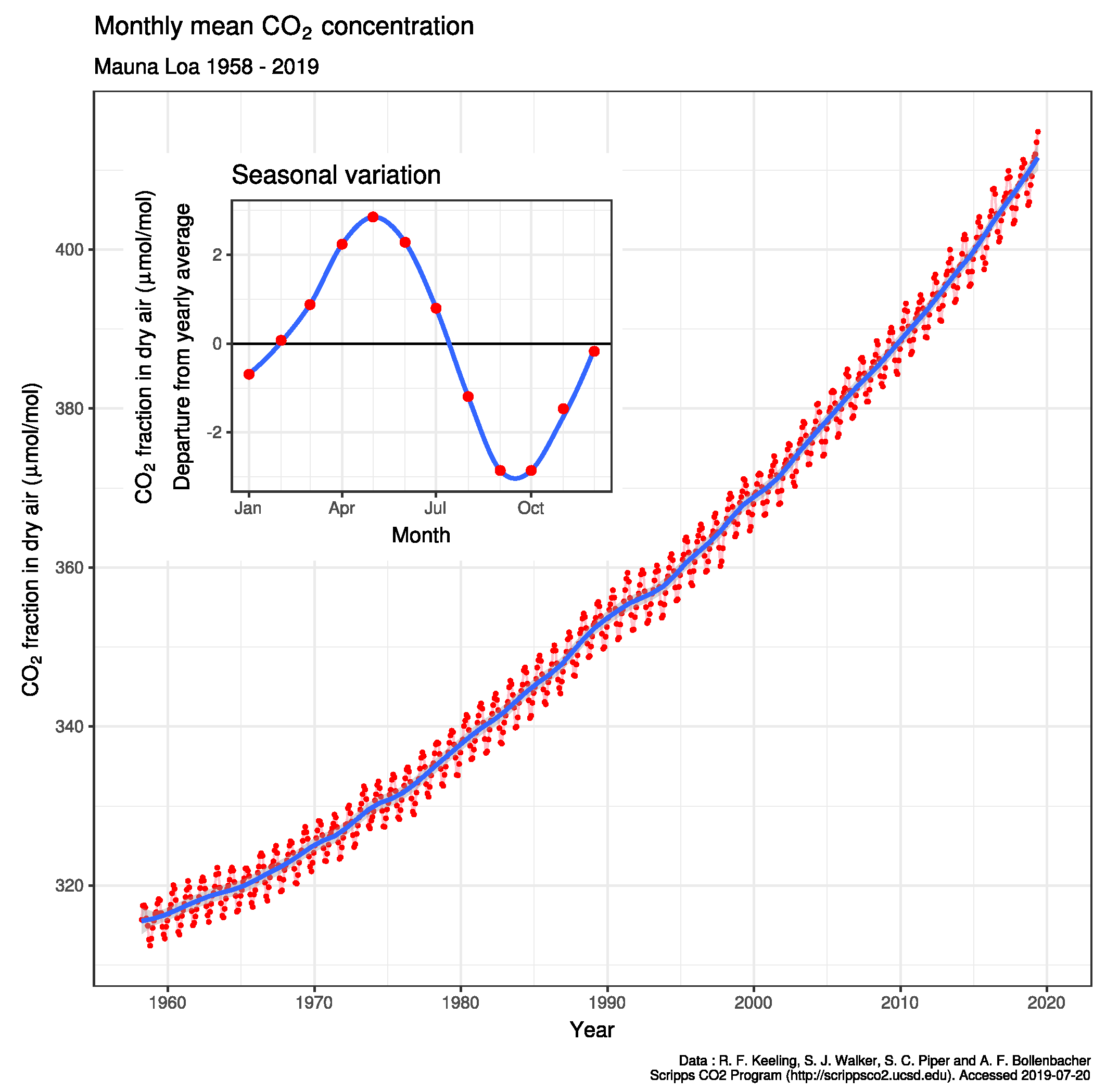
Figure 2.
Terrestrial titration hypothesis from strong acid causing increasing pCO2. in air. As pH decreases from strong acid production by oxidation of reduced sulphur and nitrogen, the DIC equilibria move towards CO2 formation, though pH changes more slowly if nearer pK values. As we have shown [1], as T varies, KSP, K1, K2, Ko, KSP vary, towards carbonate (c) and solid CaCO3 if warmer and towards bicarbonate and dissolved CO2 (a) if colder.
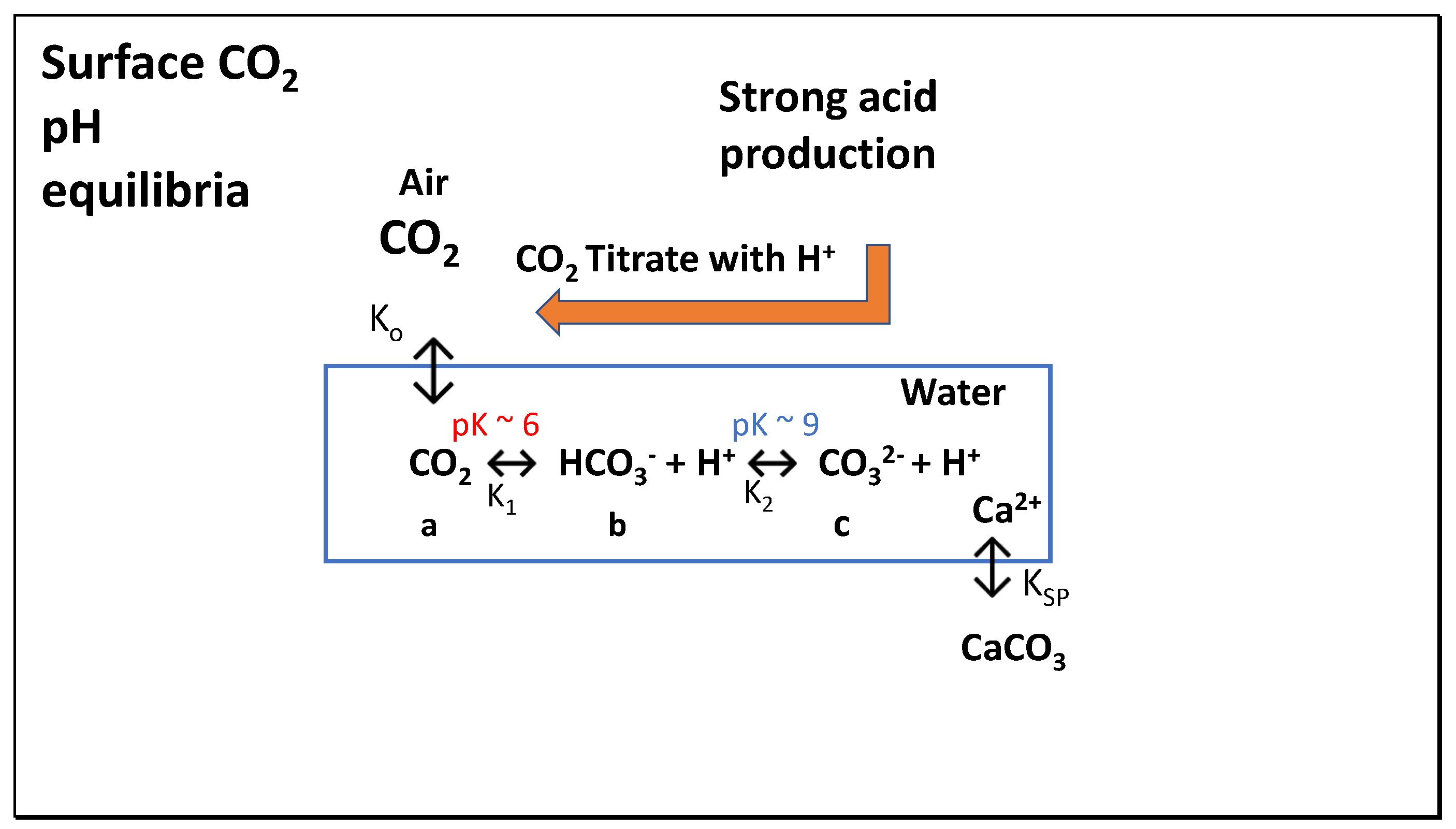
Figure 3.
Flow sheet for the CO2 Titrate program. The model allocates acidity to titrating alkalinity of carbonate and bicarbonate according to their relative concentrations at the current pH value. The Program includes a novel quadratic equation to solve for bicarbonate (b) concentration responding to inputs of other forms of DIC. Program details are given in Supplementary Materials.
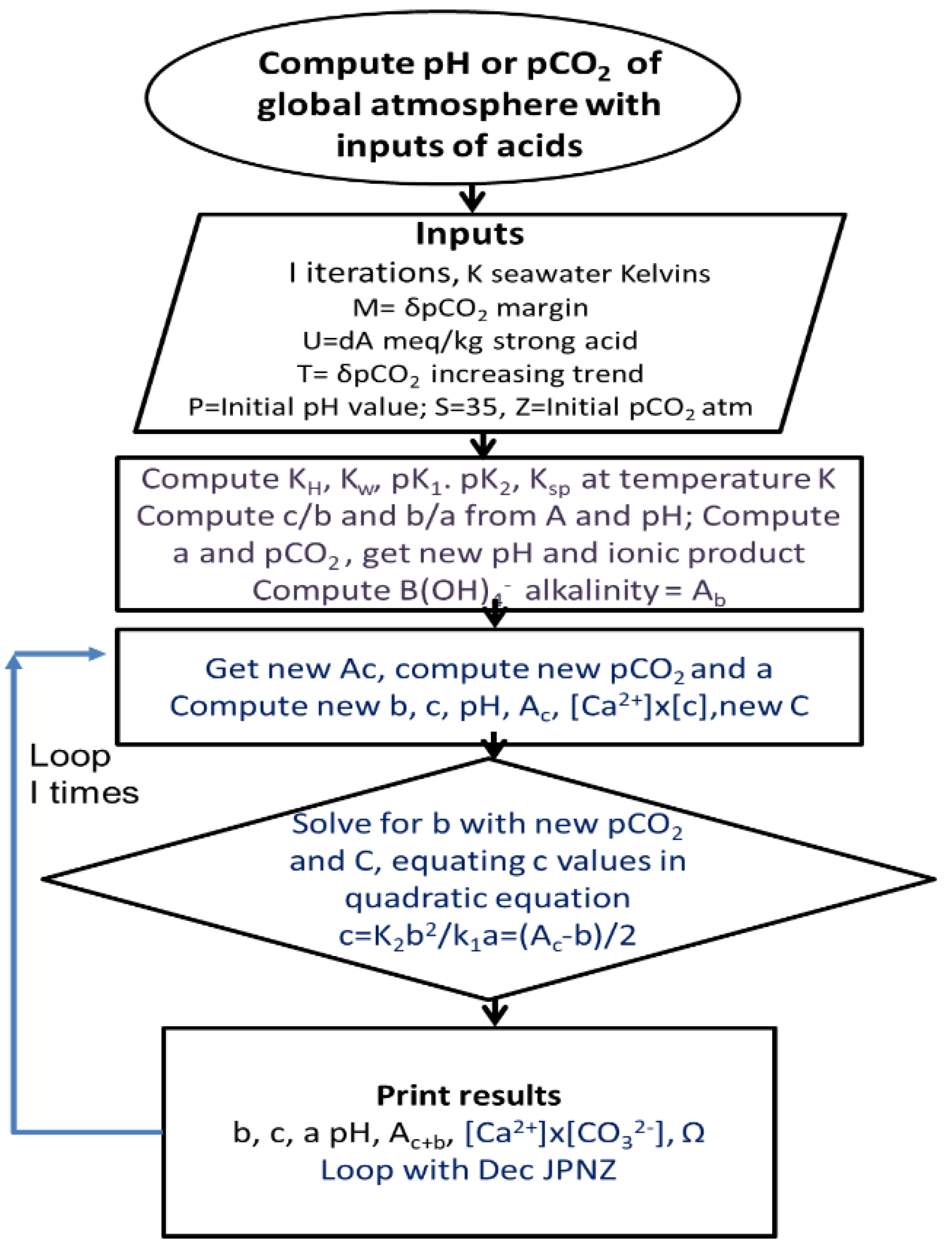
Figure 4.
Bjerrum diagram showing distribution of DIC species with pH maintaining the same DIC concentration at all pH values. Note the shift in freshwater towards more alkaline pH values for bicarbonate and carbonate pK values. This means that carbonate concentration is less at pH 8 in freshwater than in seawater and that CO2 from reaction of strong acid with bicarbonate is more nearly stoichiometric (i.e., 1:1). This figure is given by Jack J. Middelburg, 2019, Chapter 5 in Biogeochemical processes and inorganic carbon dynamics, doi: 10.1007/978-3-030-10822-9_5.
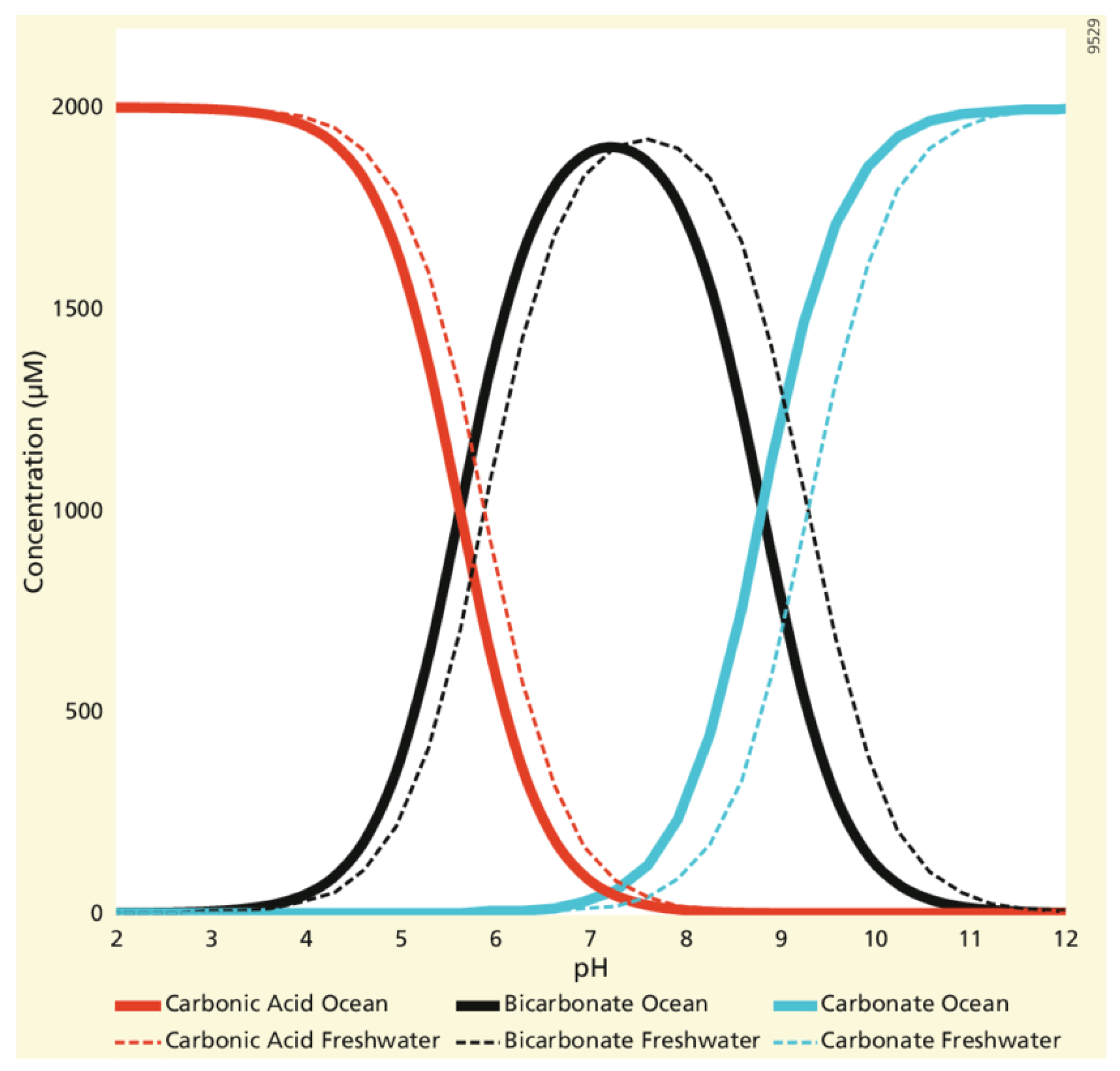
Figure 5.
Time course for DIC (C, Y-axis μmoles/kg) and carbon alkalinity (Ac, Y-axis μequiv/kg) generated by increasing pCO2 (blue, orange, 20 ppm/10 yr) or by titration with strong acid (grey, yellow, 66.5 μequiv/kg/10 yr). The complete data set is given in Table S2, Supplementary Materials.
Figure 5.
Time course for DIC (C, Y-axis μmoles/kg) and carbon alkalinity (Ac, Y-axis μequiv/kg) generated by increasing pCO2 (blue, orange, 20 ppm/10 yr) or by titration with strong acid (grey, yellow, 66.5 μequiv/kg/10 yr). The complete data set is given in Table S2, Supplementary Materials.
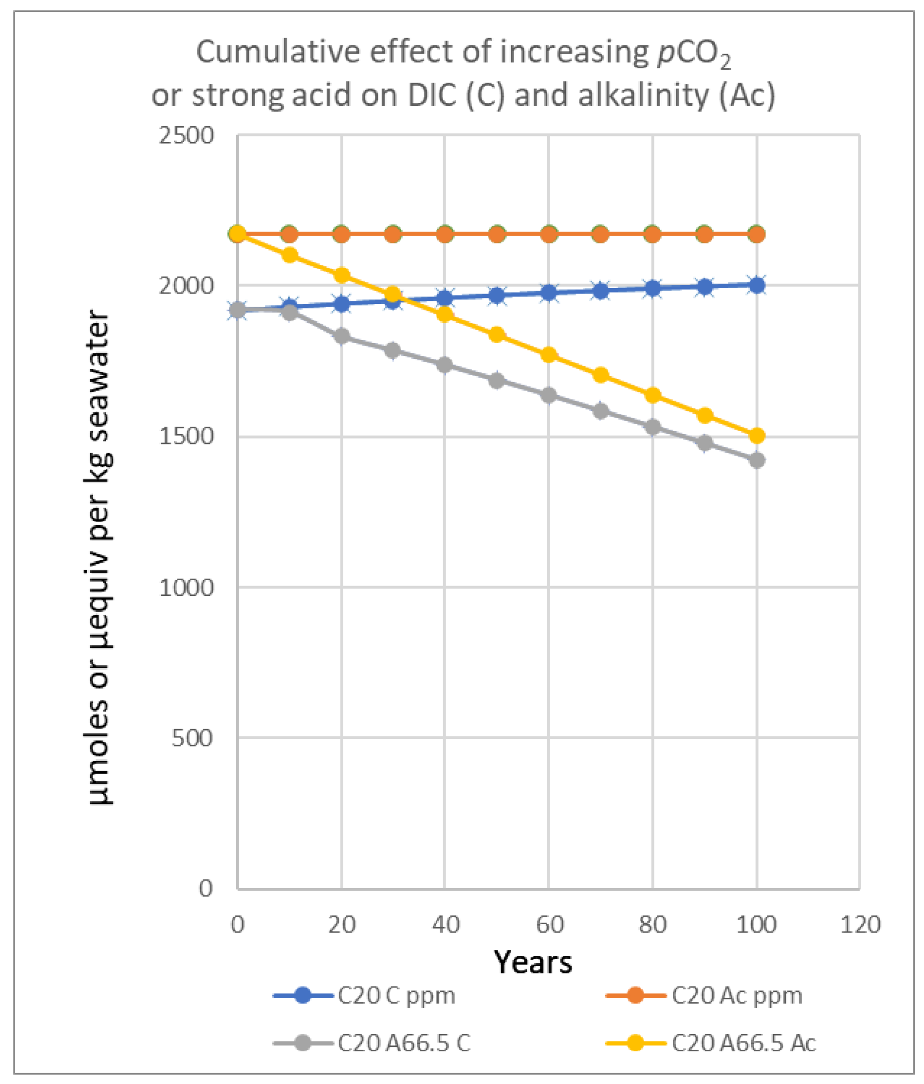
Figure 6.
Time courses (X-axis, years) for CO2 (C), strong acid (A) or calcite (L) titrations (μequiv/kg), generating increased pCO2 values (Y-axis ppmv). Primary data including a, b, c, C, Ac, Ab, Ω is included in Supplementary Materials Table S3.
Figure 6.
Time courses (X-axis, years) for CO2 (C), strong acid (A) or calcite (L) titrations (μequiv/kg), generating increased pCO2 values (Y-axis ppmv). Primary data including a, b, c, C, Ac, Ab, Ω is included in Supplementary Materials Table S3.
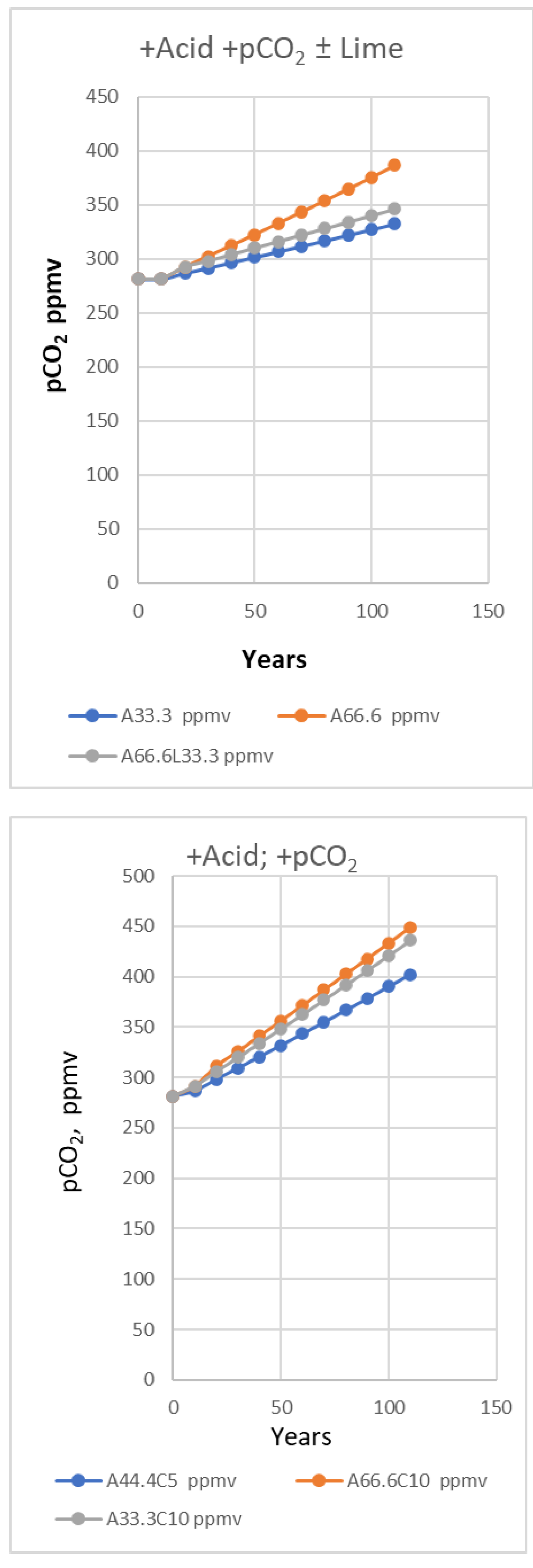
Figure 7.
Effect of strong acid on solubility of calcite (33.3 acid plus 10 ppmv, 33.3 acid or 66.6 acid μequiv/kg per 10 years).
Figure 7.
Effect of strong acid on solubility of calcite (33.3 acid plus 10 ppmv, 33.3 acid or 66.6 acid μequiv/kg per 10 years).
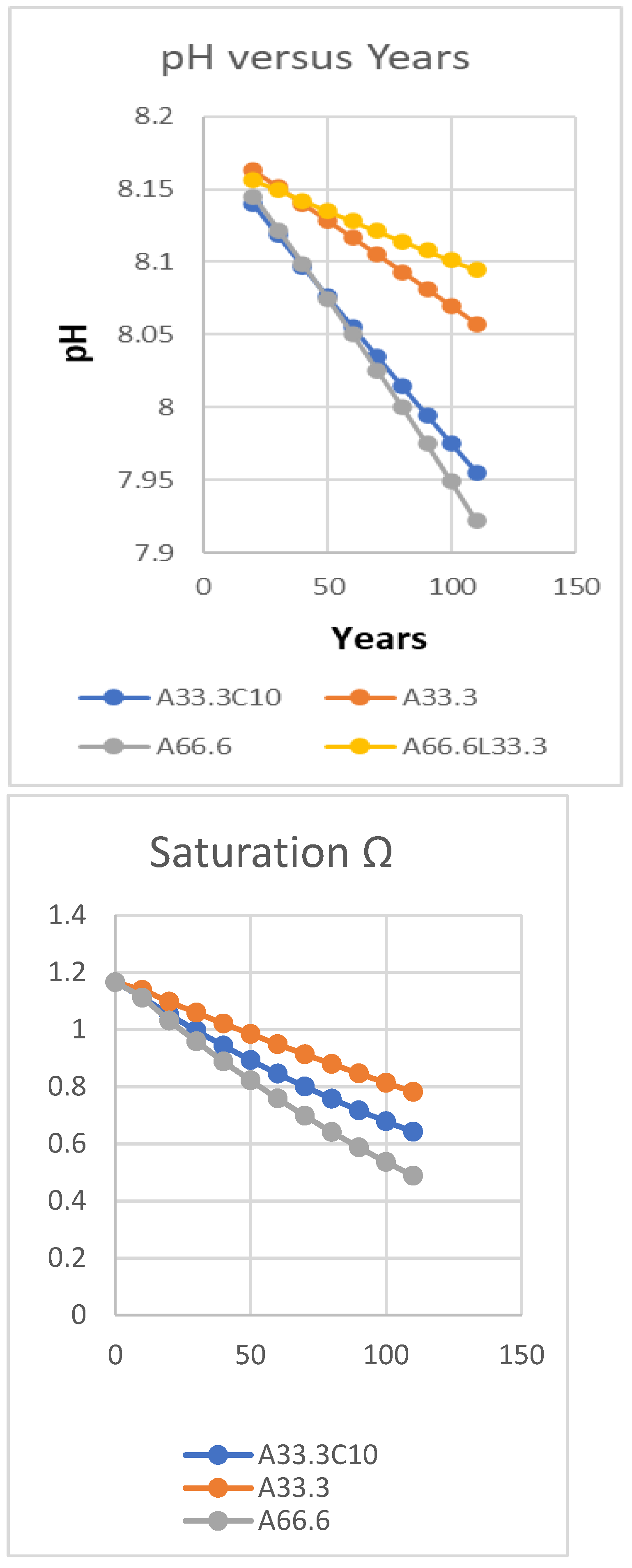
Figure 8.
Effect of increasing pCO2 (5, 10, 20 ppmv per 10 years) om seawater pH.
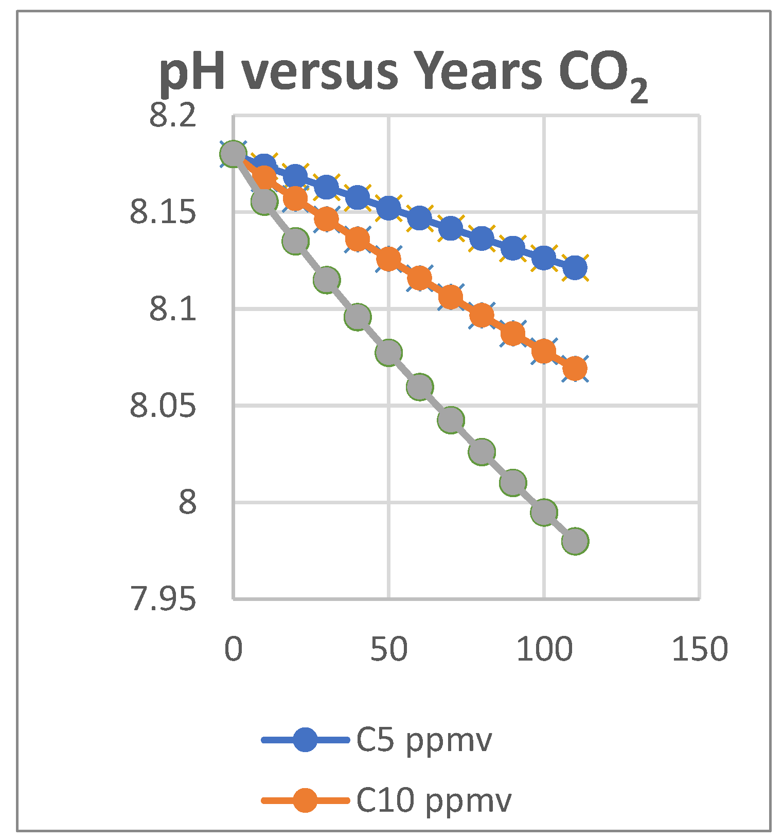
Figure 9.
Strong acidification of soil in plant growth. Protons (H+) are excreted in proportion to the extent that nutrient cations exceed anions taken up by plants. If plant or animal produce is then exported, soils in the rural environment will be acidified in proportion. Applying powdered limestone on farms releases CO2 to air.
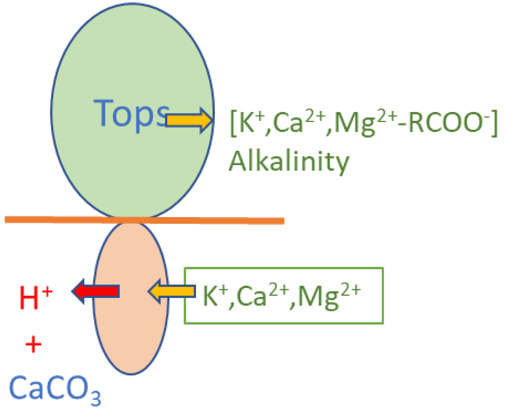
Figure 10.
Acidification from nitrogen cycling and export of produce in dairy farming with nitrogen supplied as ammonium sulphate [4].
Figure 10.
Acidification from nitrogen cycling and export of produce in dairy farming with nitrogen supplied as ammonium sulphate [4].
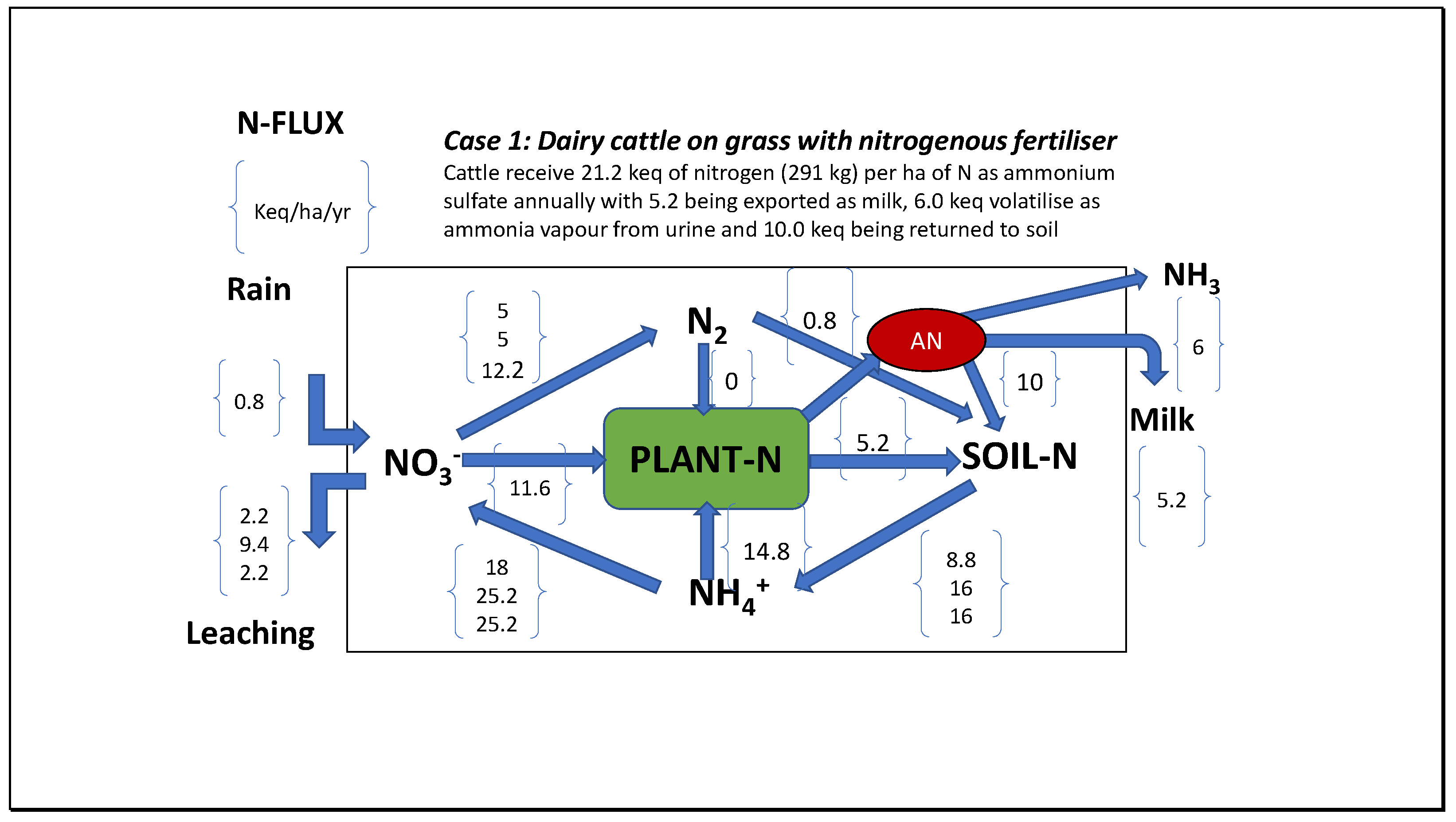
Figure 11.
Cycling of CO2 in natural ecosystems is locally balanced, its weak acidity in plants balanced by the alkalinity of reduced nitrogen; however, CO2 emission from soil follows by direct reaction with strong acid excreted from roots in exchange for nutrient cations, either by reaction with bicarbonate or with powdered limestone in soils below pH 5. The Earth’s ocean and land surface is 5.101x10¹⁴ square metres.
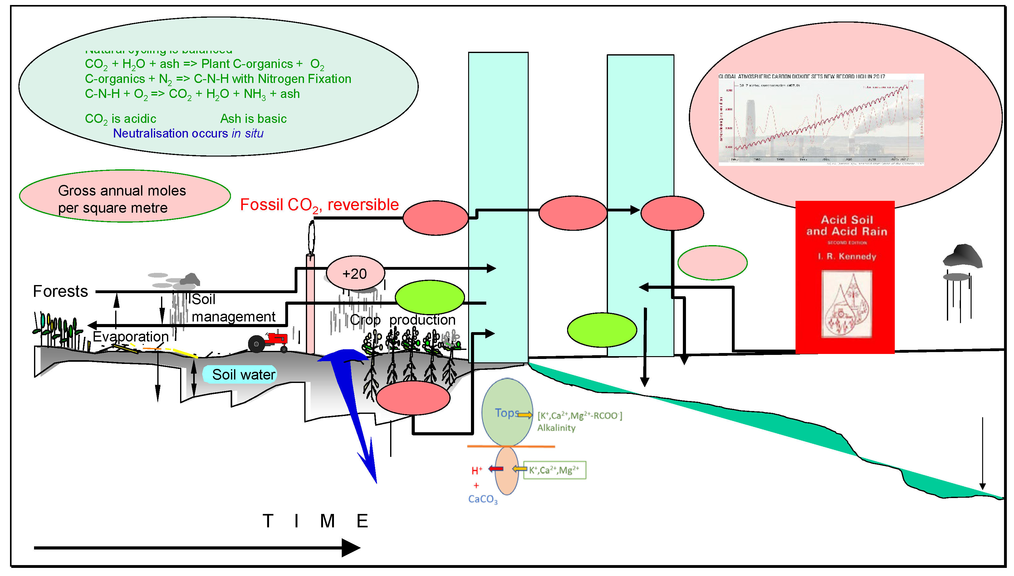
Figure 12.
FAO world map of surface soil pH and crop harvesting [48] showing a preponderance of soils with significant concentration of bicarbonate. evolving CO2 from strong acid production; FAO Harmonized world soil database (2009).
Figure 12.
FAO world map of surface soil pH and crop harvesting [48] showing a preponderance of soils with significant concentration of bicarbonate. evolving CO2 from strong acid production; FAO Harmonized world soil database (2009).
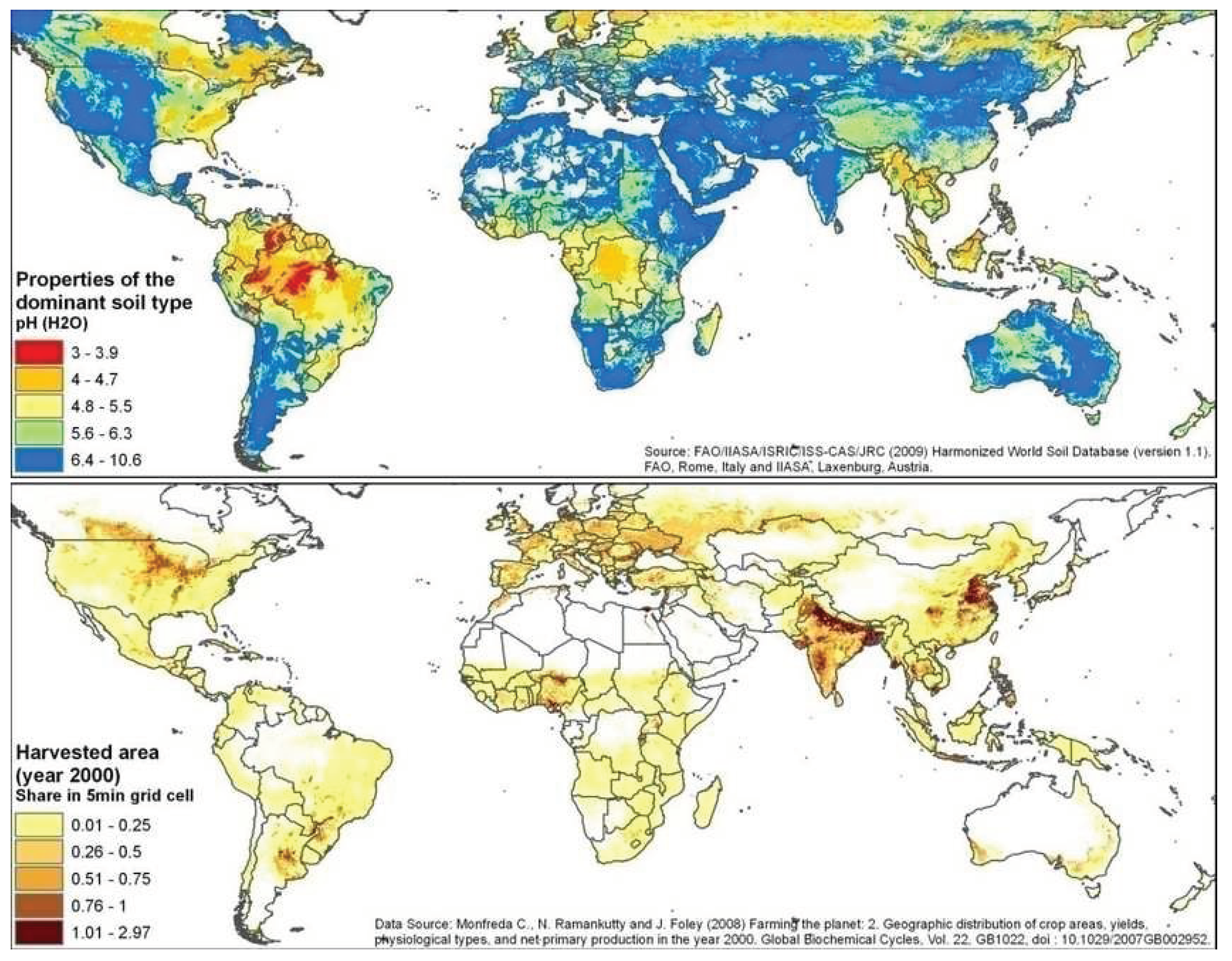
Table 1.
Increasing anthropogenic atmospheric CO2 content.
| Year | ppmv. | Moles atmospheric CO2/m2 | Increase moles/m2 | Total global atmospheric CO2 Teratonnes (1012) |
|---|---|---|---|---|
| 1750 | 280 | 95.61 | 0 | 2.1459 |
| 2020 | 420 | 140.00 | 44.390 | 3.1422 |
510.1 million km2 global surface area; 148.326 million km2 land area.
Table 2.
Total anthropogenic CO2 emissions from sulphur in fossil fuels since 1750.
| Fuel | Tonnes | Gram CO2 | Moles C | Moles S (5%) | Moles SO2/m2 | Total acidic moles CO2/m2 |
|---|---|---|---|---|---|---|
| Total global CO2 emissions | 2.5x10¹² | 2.5x10¹⁸ | 5.682x10¹⁶ | 2.841x10¹⁵ | 2.0889* | 4.19 |
| StatisticaTM 2020 annual emissions CO2 | 3.68x10¹⁰ | 3.68x10¹⁶ | 8.364x10¹⁴ | 4.182x10¹³ | 0.082* | 0.164 |
https://www.statista.com/statistics/264699/worldwide-co2-emissions/. Earth is 510.1 million km2 global area; *multiply by 6.0 to estimate ppmv; 1.48326x10¹⁴ m2 global land area.
Table 3.
Effect of titration of seawater by increasing pCO2 temperature affecting pH and calcite precipitation. Initial conditions T=278.15 K, pH 8.15, Ac=2.17 mM, S=35‰, δpCO2=2 ppmv Ksp= 4.309x10⁻⁷; program CO2TIT1.
Table 3.
Effect of titration of seawater by increasing pCO2 temperature affecting pH and calcite precipitation. Initial conditions T=278.15 K, pH 8.15, Ac=2.17 mM, S=35‰, δpCO2=2 ppmv Ksp= 4.309x10⁻⁷; program CO2TIT1.
| Years | 0 | 20 | 40 | 60 | 80 | 100 | |||||||
| [Ca2+]x[CO32-] | 5.12x10⁻⁷ | 4.25 x10⁻⁷ | 3.51x10⁻⁷ | 2.88x10⁻⁷ | 2.35x10⁻⁷ | 1.90x10⁻⁷ | |||||||
| Ω | 0.6287 | 0.5668 | 0.5162 | 0.4739 | 0.4381 | 0.4073 | |||||||
| pCO2 | 283.3 | 323.3 | 363.3 | 403.3 | 443.3 | 483.3 | |||||||
| pH | 8.15 | 8.08 | 8.01 | 7.95 | 7.88 | 7.82 | |||||||
| Initial conditions T=288.15 K, pH 8.15, Ac=2.17 mM, S=35‰, δpCO2=2 ppmv Ksp= 4.315x10⁻⁷ | |||||||||||||
| [Ca2+]x[CO32-] | 3.81x10⁻⁷ | 3.47x10⁻⁷ | 3.19x10⁻⁷ | 2.95x10⁻⁷ | 2.75x10⁻⁷ | 2.57x10⁻⁷ | |||||||
| Ω | 0.8825 | 0.8044 | 0.7938 | 0.6843 | 0.6369 | 0.5958 | |||||||
| pCO2 | 287.4 | 327.4 | 367.4 | 407.4 | 447.4 | 487.4 | |||||||
| pH | 8.15 | 8.10 | 8.06 | 8.02 | 7.98 | 7.95 | |||||||
| Initial conditions T=298.15 K, pH 8.15, Ac=2.17 mM, S=35‰, δpCO2=2 ppmv Ksp= 4.272x10⁻⁷. | |||||||||||||
| [Ca2+]x[CO32] | 5.12x10⁻⁷ | 4.71x10⁻⁷ | 4.37x10⁻⁷ | 4.07x10⁻⁷ | 3.82x10⁻⁷ | 3.59x10⁻⁷ | |||||||
| Ω | 1.1988 | 1.0351 | 1.0228 | 0.9354 | 0.8933 | 0.8404 | |||||||
| pCO2 | 283.3 | 323.3 | 363.4 | 403.4 | 443.4 | 483.4 | |||||||
| pH | 8.15 | 8.10 | 8.06 | 8.02 | 7.99 | 7.96 | |||||||
Table 4.
Equilibrium concentrations of DIC in seawater (S=35) and land water (S=0.35) at given pH values and salt. concentrations (temperature 288 K, pCO2=420 ppmv).
Table 4.
Equilibrium concentrations of DIC in seawater (S=35) and land water (S=0.35) at given pH values and salt. concentrations (temperature 288 K, pCO2=420 ppmv).
| Salt (NaCl ‰) | 35 | 35 | 35 | 35 | 0.35 | 0.35 | 0.35 | 0.35 |
| pH | 8.2 | 7.2 | 6.2 | 5.2 | 8.2 | 7.2 | 6.2 | 5.2 |
| [CO2] μM = a | 15.8 | 15.8 | 15.8 | 15.8 | 19.2 | 19.2 | 19.2 | 19.2 |
| [HCO3-] μM = b | 2930.2 | 293.0 | 29.3 | 0.93 | 1924.7 | 192.5 | 19.2 | 1.92 |
| [CO32-] μM = c | 352.1 | 0.35 | 0.0004 | 0.000 | 74.3 | 0.07 | 0.001 | 0.000 |
| [HCO3-]/[CO32-] | 8.27 | 82.7 | 827.4 | 8274.4 | 25.7 | 257.5 | 2574.9 | 25749.1 |
| C=a+b+c μM | 3298.1 | 312.3 | 45.1 | 16.7 | 2018.2 | 217.4 | 38.4 | 21.12 |
Computed using the CO2TIT4 program given in Table S in Supplementary Materials.
Table 5.
Titrate distributions for dissolved inorganic carbon in seawater and pCO2 values, given inputs of temperature, pH value and alkalinity (μequiv/kg).
Table 5.
Titrate distributions for dissolved inorganic carbon in seawater and pCO2 values, given inputs of temperature, pH value and alkalinity (μequiv/kg).
| Kelvin | pH | Ac | [CO2]=a | [HCO3-]=b | [CO32-]=c | C | pCO2 | Ω |
| 278.15 | 8.15 | 2170 | 14.802 | 1896.349 | 136.826 | 2047.976 | 283.9 | 0.629 |
| 278.15 | 8.15 | 2000 | 13.642 | 1747.787 | 126.107 | 1887.536 | 261.7 | 0.579 |
| 278.15 | 8.25 | 2170 | 11.386 | 1836.387 | 166.807 | 2014.579 | 218.4 | 0.766 |
| 278.15 | 8.25 | 2000 | 10.494 | 1692.252 | 153.739 | 1856.755 | 201.3 | 0.706 |
| 288.15 | 8.15 | 2170 | 10.767 | 1785.386 | 192.307 | 1988.460 | 287.4 | 0.883 |
| 298.15 | 8.15 | 2170 | 8.043 | 1652.623 | 258.688 | 1919.354 | 283.3 | 1.200 |
Table 6.
Crude estimates for annual global generation of environmental acids for 2021.
| Acid | Source | Estimated total moles H+ and CO2 | Annual acid meq/m2 globally |
| Hydrogen ions (H+) | Croplands, 15x1012 m2 sown alkalinity export | 10.0x10¹² | 19.6 |
| “ | Forestry, 50x1012 m2 harvested alkalinity export | 5.0x10¹² | 9.8 |
| “ | Rangelands, 100x1012 m2 alkalinity export | 5.0x10¹² | 9.8 |
| Nitric, HNO3 | Nitrification of NH3 and excess legume-N | 17.5x10¹² | 39.2 |
| Agriculture total | 37.5 | 73.6 | |
| Sulphuric, H2SO4 | Coal, oil, gas, wood combustion | 16x1012 | 64.0 |
| Sulphuric, H2SO4 or sulphurous | Anaerobic sulphate respiration [4] from ca. 1013 moles C annually in sewage, discharged mainly to the ocean; UV oxidation H2S and DMS [4]; oxidation of sulphides in aerated acid sulphate soils after drainage for urban habitation [24] | 25x1012 | 98.0 |
| Carbonic acid H2CO3 | Global respiration = assumed photosynthesis | 17,500x1012 | 34,307.0 |
| Carbonic acid “ | Coal, oil and gas fossil emissions | 816x1012 | 1,599.7 |
| Carbonic acid “ | Increasing wildfires with population | 100x1012 | 392.1 |
| Nitric, sulphuric, acids | From increasing combustion in wildfires, ash countering acidification in forests | 12x1012 | 25.9 |
| Carbonic acid H2CO3 | Cement, construction | 104.6 | |
| Total emissions | Approximate estimate only ±10% | 36,261.3 | |
| Weak acid | H2CO3 | pK 6.5, 8.9 | 35,947.2 |
| Total strong acids (H+) | C-fuels, agriculture, fire, smelting ores with sulphides (20 mequiv/m2) | pK ca. 0-1 | 336.6 |
| Wildfires 1.76 billion tonnes | |||
| Scenario 1 | 2.5% greater photosynthesis annually | +438x1012 | |
| Photosynthesis | All sources + CO2 fertilisation | 17,938x1012 | -35,164.7 |
| Net CO2 | Respiration – new photosynthesis | -438x1012 | -1,072.3 |
| CO2 to atmosphere | Current increase per annum 2.5 ppmv | 833.0 | |
| CO2 at surface | Seawater, land water emission | 239.0 | |
| Scenario 2 | 1% greater photosynthesis annually | +175x1012 | 343.1 |
| Photosynthesis | All sources + CO2 fertilisation | 17,675x1012 | -34,650.1 |
| Net CO2 | Weak acid - photosynthesis | 175x1012 | -1297.1 |
| CO2 to atmosphere | Current increase per annum 2.5 ppmv | 833.0 | |
| CO2 at surface | Seawater, landwater uptake | 464.1 |
Total weak and strong acid production is estimated annually of as CO2 per square metre. Each square metre now has ca. 140 moles CO2 in the air column to space at 420 ppmv over a total area of 5.101x10¹⁴ m2. From FAO data, ca. 40% of 6x10¹³ m2 total of land is devoted to agriculture and ca. 2x10¹³ m2 to crops, say half exported away from soil; potential dimethylsulfide (DMS) or related reduced sulphur emissions, oxidised rapidly in air, absorbed by seawater; a change of 1 ppmv of CO2 in air is equivalent to 2.13 Gt C globally.
Table 7.
Summary of sources of global annual atmospheric CO2 emissions.
| Acidifying process | Moles of global strong acid production | Moles of CO2 increase (meq/m2) |
Statistical confidence |
| Increase in atmospheric CO2 (2021) | 664.0x10¹² | Strong | |
| Sources of strong acid production | Sulphuric, nitric | ||
| Fossil fuels (2% fossil CO2 moles untrapped SO2) | 32.8x10¹² | 64.0±10 | Moderate |
| Acidification from agriculture and forestry | 37.5x10¹² | 73.6±10 | Moderate |
| Increasing wildfire acidification S and N | 44x1012 | 81.3±20 | Low |
| Anaerobic sulphate respiration, H2S, DMS | 25x1012 | 98.0±20 | Low |
| Mining exposure, refining metal, sulfides, pyrites | 10x1012 | 20.0±50 | Low |
| Total decrease in alkalinity from strong acids | 197x1012 | 336.6±110 | Approximate |
Disclaimer/Publisher’s Note: The statements, opinions and data contained in all publications are solely those of the individual author(s) and contributor(s) and not of MDPI and/or the editor(s). MDPI and/or the editor(s) disclaim responsibility for any injury to people or property resulting from any ideas, methods, instructions or products referred to in the content. |
© 2024 by the authors. Licensee MDPI, Basel, Switzerland. This article is an open access article distributed under the terms and conditions of the Creative Commons Attribution (CC BY) license (http://creativecommons.org/licenses/by/4.0/).
Copyright: This open access article is published under a Creative Commons CC BY 4.0 license, which permit the free download, distribution, and reuse, provided that the author and preprint are cited in any reuse.


