Submitted:
20 March 2024
Posted:
26 March 2024
You are already at the latest version
Abstract
Euler-Poisson equations of a charged symmetrical body in external constant and homogeneous electric and magnetic fields are deduced starting from the variational problem, where the body is considered as a system of charged point particles subject to holonomic constraints. The final equations are written for the center-of mass-coordinate, rotation matrix and angular velocity. General solution to the equations of motion is obtained for the case of a charged ball. For the case of a symmetrical charged body (solenoid), the task of obtaining the general solution is reduced to the problem of a one-dimensional cubic pseudo-oscillator. Besides, we present a one-parametric family of solutions to the problem in elementary functions.
Keywords:
Euler-Poisson equations
; exact solutions in elementary functions
; constrained systems
; integrable systems
; spinning body in external fields
1. Introduction
Spinning bodies represent an important object of study in modern research at different scales, from problems of approaching compact stars in gravitational wave physics to levitating nano-particles and elementary particles with spin. Behavior of a spinning object in special and general relativity as well as in quantum mechanics in many cases is considered in first order by perturbation theory based on exact solutions to the classical problem [1]. Therefore, the search for new integrable cases and analytical solutions in the dynamics of a spinning body is important for further progress in such problems. In the present work we consider a charged spinning body in external constant and homogeneous electric and magnetic fields. While the case of a ferromagnet has been discussed quite widely in the literature [2,3,4,5,6,7], much less attention has been paid to a charged dielectric [8]. In this article we will try to fill this gap in the literature.
The work is organized as follows. In Section 2 we deduce equations of motion on the base of a Lagrangian action, formulated for the case under consideration. We will present a detailed derivation of the equations, since semi-empirical methods applied to a spinning body in some cases lead to either inaccuracies or erroneous interpretation of the final result. In Section 3 we present general solution to obtained equations for the case of a charged ball. In Section 4 we reduce the problem of a symmetrical charged body to the problem of a one-dimensional non-linear pseudo-oscillator. In Section 5 we present a one-parametric family of solutions in elementary functions for the motions with specially chosen initial angular velocity of the symmetrical charged body. In the Appendix, for the convenience of the reader, we summarized the motion of a point charged particle in external electromagnetic field.
2. Charged Body in Constant and Homogeneous Electric and Magnetic Fields
Consider a rigid body that consist of n particles of charge and mass , . Its Lagrangian action reads [9]
The first term is kinetic energy of all particles, while the remaining terms account the presence of constraints, that guarantee that distances and angles among the particles do not change with time1. The constraints were added with help of Lagrangian multipliers . In all calculations these auxiliary variables should be treated on equal footing with . In particular, looking for the equations of motion, we take variations with respect to and all . The -block of was chosen to be the symmetric matrix. The variations with respect to imply the constraints, which therefore arise as a part of conditions of extreme of the action functional. So the presence of allows to be treated as unconstrained variables, that should be varied independently in obtaining the equations of motion.
We consider the body immersed into constant and homogeneous electric and magnetic fields with scalar potential and vector potential , see Appendix. Summing up the potential energies (A15) of body’s particles, we obtain its total potential energy
Adding it to the action (1), we obtain a variational problem for the body in external electric and magnetic fields. We assume that all particles of the body have the same charge to mass ratio, for any . Then our action implies the following dynamical equations
Introducing the center of mass, , where , the equations (3) imply
that is center-of-mass behaves like charged point particle discussed in Appendix. In particular, rotational motion of the body does not affect its translational motion.
Substituting into Eq. (3) and taking into account (4), we rewrite these equations in the center-of-mass coordinate system
Each solution to these equations is of the form , where is an orthogonal matrix that, by construction, obeys the universal initial data . Substituting this expression into Eqs. (5), then multiplying the equation with number N by and taking their sum, we obtain the following second-order equations for determining the rotation matrix :
It was denoted
Besides, is the mass matrix
while is the symmetric matrix
where all are taken at the instant .
Due to the identity , satisfied for the center-of-mass coordinates, second term on r. h. s. of Eq. (6) vanishes. In the result, the electric field do not affect the motion of rotational degrees of freedom. Besides, the center-of-mass variable do not enter into this equation, so the translational motion does not affect the rotational motion of the body.
The variables in equations (6) depend on the unknown dynamical variables . Fortunately, we do not need to know , because of these equations determine algebraically, as some functions of R and . This result, obtained with use of the procedure described in [9], can be formulated as follows
Affirmation. Consider the second-order system for determining the variables and
where is some given matrix that does not depend on and (as before, is a numerical symmetric non-degenerate matrix, and ).
The problem (10) is equivalent to the following Cauchy problem for the first-order system, written for the mutually independent variables and :
where I is inertia tensor of the body with the components .
Note that this system is composed of vectors and tensors, so it is covariant under the rotations. We will work with these equations assuming that the mass matrix and inertia tensor are of diagonal form. This implies [9], that at initial instant the Laboratory basis vectors were taken in the directions of axes of inertia taken as the body-fixed frame: . We also recall that the body-fixed basis vectors are columns of the rotation matrix: . Eigenvalues of mass matrix and inertia tensor are related as follows: , and so on.
Our equations (6) are of the form (10), so they are equivalent to the first-order system (11) and (12) with A written in (7). To obtain an explicit form of Eq. (11), we use (12) to rewrite the quantity as follows:
Thus
Using the latter expression for in Eq. (11), after direct calculations this acquires the form
The vector composed of last three terms can be written in a more compact form in terms of the mass matrix. Indeed, writing the first component of this vector in explicit form we get
and similar expressions for the second and third components. Then Eq. (11) acquires the final form
For completeness we also present equations for the vector of angular momentum and for its components in the body-fixed frame
Let us consider Eqs. (16) in the Laboratory system with third axis in the direction of magnetic vector . Denote by and the non diagonal tensors of inertia and mass that will appear in this coordinates. Then Eqs. (16) acquire the form , where is the third row of the rotation matrix . They coincide with those deduced by G. Grioli, see [1,8].
In resume, we have succeeded in obtaining equations of motion (16), (12) and (4) for a spinning charged body in external electric and magnetic fields. The solution , to these equations contains complete information on the evolution of the body with respect to Laboratory frame: dynamics of the body’s point with initial position is .
3. General Solution to the Equations of a Charged Ball
Consider a totally symmetric charged body:
This could be a charged ball. Then its center moves according to Eq. (A13). From kinematic relations between angular momentum , angular velocity and its components in the body-fixed frame, together with Eq. (19), we get . The first equality means that for all t the instantaneous rotation axis remains parallel with the vector of angular momentum. Substituting (19) into equations of previous section, we get
The last equation implies that angular momentum precesses around with Larmor’s frequency . Besides, the length of angular momentum and its projection on -axis are first integrals
Components of angular velocity with respect to body-fixed frame precess with the same frequency around the components of magnetic field in body-fixed frame.
Substituting into (21) and taking into account (20), we arrive at the equation (22). So the system (20), (21) is equivalent to , . Further, the first (non linear on R) equation of latter system can be replaced on the linear equation . The resulting system an the initial one have the same solutions in the set of orthogonal matrices. In the result, instead of Eqs. (20) and (21), a totally symmetric body can be described by the equations
where all quantities are defined with respect to the Laboratory system. The initial conditions are . According to these equations, precesses around constant vector , while the vectors instantaneously precess around .
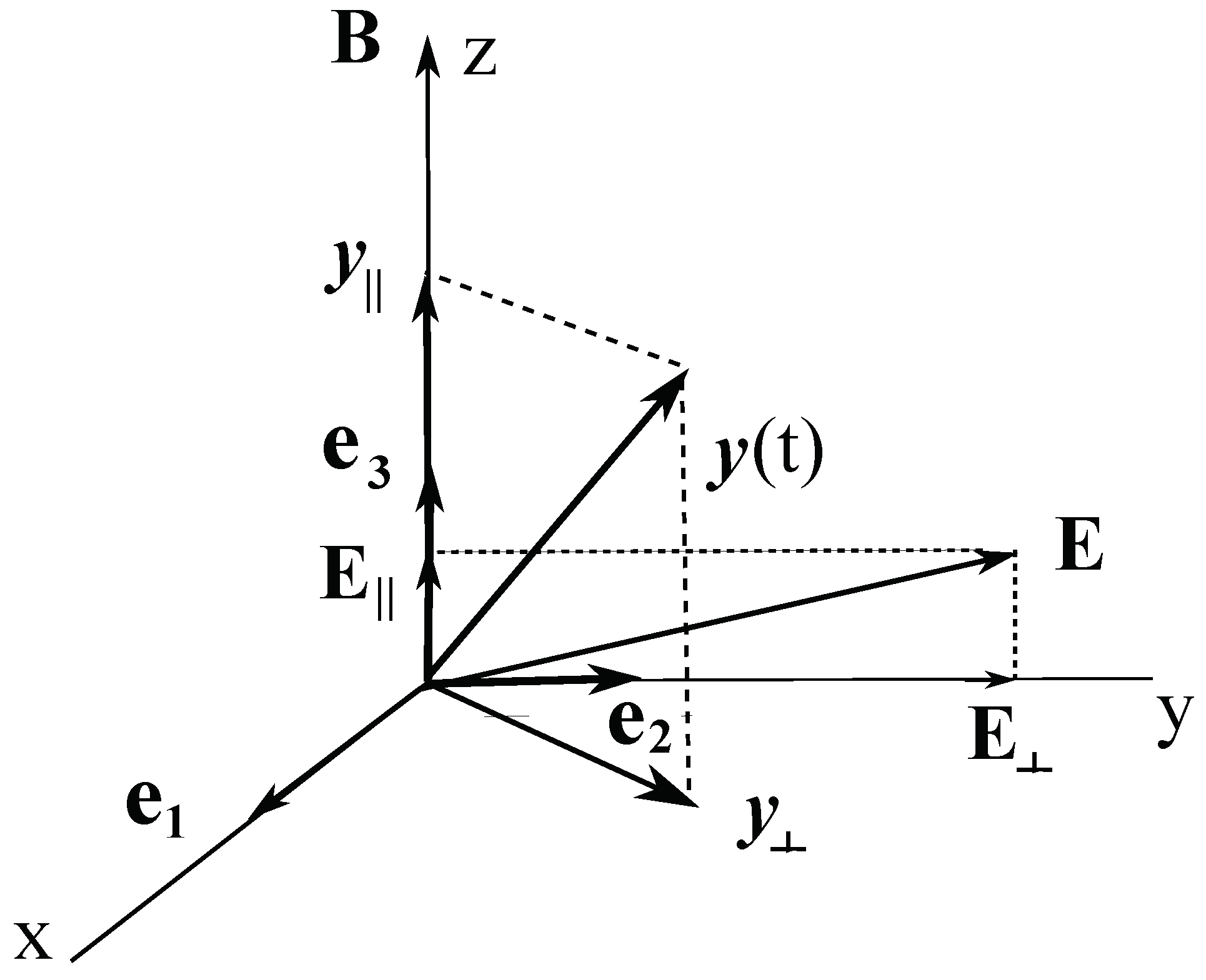
Let us obtain the general solution to the system (24), (25). For a totally symmetric body we can choose the directions of Laboratory axes as convenient, this will not violate the diagonal form of inertia tensor. Using this freedom, we choose the Laboratory system so that at the vectors and lie in the plane of , and , and is directed along , see Figure 1.
Then , , and
is a solution to Eq. (25), where the precession frequency is the Larmor’s frequency
To solve Eq. (24) with this , we write it as follows: . We look for a solution to Eq. (24) in the form
To fix and , we substitute the ansatz (28) into (24) an then take in the resulting expressions. They determine as follows: , . Then implies . The obtained equalities allow us to represent and through and as follows:
By direct calculations, it can be verified that the expression (28) with these and satisfies the equations (24).
In resume, we obtained analytical solution for a charged ball launched with initial angular velocity in constant and homogeneous electric and magnetic fields. It is given by the double-frequency rotation matrix (28), (29). The total motion can be thought as a superposition of two rotations: the first around unit vector with the frequency , and the second around the axis of magnetic field with the frequency . The angular momentum vector precesses around the vector with the Larmor’s frequency .
Let us consider the ball launched with initial vector of angular velocity parallel to the vector of magnetic field . That is the initial conditions are . Then , and . With these values, the rotation matrix (28) reduces to
As it should be expected, the ball experiences a stationary rotation around the vector of magnetic field with the frequency .
4. Symmetrical Charged Body and One-Dimensional Non Linear Pseudo-Oscillator
In this section we start to study the symmetrical charged body. We show that for any solution , to Euler-Poisson equations, the function obeys to the equation of a one-dimensional cubic pseudo-oscillator, see Eq. (47) below. Besides, when is known, the functions and can be found by quadratures, see Eqs. (44) and (45).
Consider Eqs. (12) and (16) for the symmetrical body2: . This implies the following mass matrix: . We consider the positively charged body, then the charge-mass ratio is a positive number, . We assume that at the third inertia axis of the body is vertical. Then, without spoiling the diagonal form of inertia tensor in our equations, the Laboratory system can be chosen as shown on Figure 2.
The basis vector is directed along the third inertia axis , the vectors and lie on the plane of paper sheet together with the vector of constant magnetic field . The initial instantaneous angular velocity of the body is
It is convenient to introduce the following notation:
Contracting the Poisson equations (12) with , we get . This equation together with (16) give us the auxiliary system of closed equations for determining the variables and
By construction, the initial conditions for are . Any solution , to Euler-Poisson equations obeys to this system. So we can use the latter to look for the angular velocity .
This system admits four integrals of motion. Two of them are
To obtain two more integrals, we write our system in components
The equations with and imply the third integral
Combining the equations with , , and we get one more integral of motion
We written them through the integrations constants and , as well as through the initial data and of the problem.
Using (40), (41) and the equation with of the system (38), we represent the variables through as follows
Substituting them into equations for and from (38), we get
where and turn out to be the following functions of :
If is known, the equations (43) can be immediately integrated as follows
where is indefinite integral of , while and are the integration constants.
So it remains to find the third component . To this aim we compute the time derivative of the last equation from (38), and use other equations of the system (38), (39) in the resulting expression, presenting it as follows
Using the integrals of motion (36), (37) and (41), we obtain closed equation for determining , that can be called the equation of cubic pseudo-oscillator
where the numeric coefficients are functions of initial data of original problem
It is not difficult to obtain a two-parametric family of simple solutions to the equation (47). Note that will be (constant) solution to (47) if the third component if initial angular velocity is a root of the third degree polynomial on the right side of (47). Substituting into Eq. (47), we obtain the condition on initial data under which satisfies this equation. To obtain this condition, it is convenient to represent Eq. (47) in terms of the initial data, keeping the combinations like as follows:
Substituting , we get that (47) will be satisfied only for the initial data obeying the following equation:
or, equivalently
This is a surface of second order. Since the point with obeys this equation, the surface always pass through the origin of coordinate system. Resolving (50) with respect to , we get the following two-parametric family of constant solutions to the equation (47) of cubic pseudo-oscillator:
Let us find out which quadric is defined by the equation (51), by writing it in the canonical form. Following the standard procedure [10], we arrive at the new coordinates :
where is the angle between the vectors and , see Figure 3. The new coordinates are obtained from by shifting the origin of coordinate system to the point , and subsequent rotation counter-clockwise by the angle in the plane . Note that . In these coordinates Eq. (51) acquires the form
Depending on the relationship between the inertia moments and , it describes different surfaces.
1. Let . This body could be a charged sufficiently short cylindrical surface. If it rotates around its coaxial axis, it will produce a magnetic field corresponding to a short solenoid. The equation (54) turn into
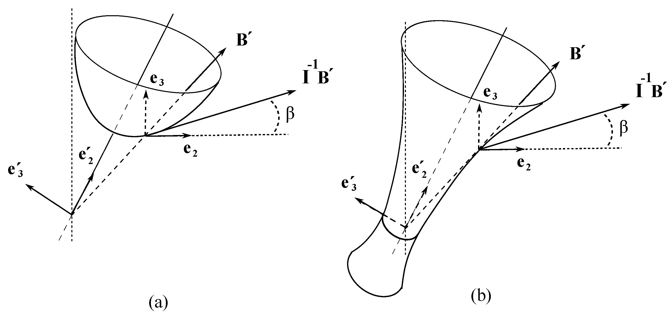
Hence the surface of initial data is a hyperboloid of two sheets. Its upper sheet is shown in Figure 3 (a).
In the limiting case we have a plane body, that could be charged circular loop. In this case the sheets of the hyperboloid are tangent to the horizontal planes and .
2. For the totally symmetric body , the equation (54) turn into the cone
with semi axes and written in equation (54).
3. Let . This body could be a charged long cylindrical surface. If it rotates around its coaxial axis, it will produce a magnetic field corresponding to a long solenoid. The equation (54) turn into
Hence the surface of initial data is a hyperboloid of one sheet shown in Figure 3 (b).
In resume, we have shown that for any solution to the Euler-Poisson equations (12) and (16) of a symmetrical charged body, the function obeys the equation of cubic pseudo-oscillator (47). We obtained a two-parameter family of constant solutions (52) to this equation. Not all of them generate solutions to the original problem. In the next section they will help us to obtain a one-parameter family of solutions to the original Euler-Poisson equations in elementary functions.
5. Rotation Matrix: One-Parameter Family of Solutions in Elementary Functions
As we saw in previous section, our problem (12), (16) probably admits solutions with constant . So let us search for solutions of the auxiliary task (34), (35) of the form
Substituting this ansatz into the equations (34) and (35), they turn into
These equations admit three integrals of motion: , and . This implies the equalities
Using the equations and we get that and are just proportional to and
Substituting these expressions into (59) and (60), we get the equations of precession
and
They will be consistent only if , that is the initial data should lie on the surface
Combining this with the necessary condition (50)
we conclude that the initial data should be taken on the curve of second-order
that lie on the plane . Geometrically, these are hyperbolas that appear as a result of the intersection of the hyperboloids in Figure 3 with this plane.
For the circular loop or short solenoid they are
For the long solenoid they are
At last, for a totally symmetric body they degenerate into the straight lines
Resolving Eq. (67) with respect to we get
With this , the two systems (63) and (64) depend on the same frequency
and imply the following solution
This means that vector of angular velocity in the body-fixed frame precesses around the third axis with the frequency .
The next step is to solve the Poisson equations (12). We consider them in the form
with specified by Eqs. (71)-(73). Here is any one of rows of the rotation matrix.
In components this reads
This system admits the integral of motion
where and are components of unit vector in the direction of magnetic vector . Preservation in time of the quantity (76) can be verified by direct computation of its time-derivative, with use the identities
We need to find the general solution to the equations (75). Then, according to [9], the rows of the rotation matrix can be obtained taking the following three particular solutions. The row is with the initial data and with . The row is with the initial data and with . At last, the row is with the initial data and with .
First we solve algebraically the equations and , representing and as follows:
Substituting them into the equation for , we get closed equation of second order for
This is equation of harmonic oscillator with constant frequency k, under the action of an external constant force. Its general solution with the integration constants b and is
Substituting this result into the expressions (78), we obtain the remaining variables
At we get
Solving the equations (82) with the data described below Eq. (77), we get, in each case
Substituting these values into Eqs. (80) and (81) we get the rotation matrix of a symmetrical charged body, immersed into the magnetic field , and launched with initial angular velocity (73)
Two frequencies in the problem are: written in Eq. (72), and . The dependence of the rotation matrix on the inertia moments , as well as on the charge-mass ratio is hidden in the frequency .
By direct substitution of obtained functions (73) and (84) into the equations (12) and (16), I verified that they are satisfied.
The rotation matrix can be decomposed as follows:
Then the position of any point of the body at the instant t is: . It is obtained by rotating the initial position vector first around the laboratory axis by the angle and then around the -axis by the angle .
It can be said that the motion is the composition of a proper rotation around third inertia axis with precession of this axis around the vector of magnetic field . The final answer (84) admits the limit of totally symmetric body , this implies . The resulting motion is the precession around the magnetic vector without a proper rotation.
Combining Eqs. (71), (72) and (79) we get the relation between two frequencies of the motion (84)
We recall that the most general motion of a free symmetrical body is the precession without nutation [9]. Observe that the rotation matrix (84) coincides with Eq. (132) of this work if we replace , and on , k and . The physical meaning of this coincidence can be formulated as follows.
Affirmation. If a symmetrical charged body in the magnetic field moves according (84) with the precession frequency around and the proper rotation frequency , then in the absence of a magnetic field its precession with the same frequency around the unit vector will happen with the proper rotation frequency
Indeed, consider the motion (84) with initial angular velocity . Let it then was launched in the absence of a magnetic field with initial angular velocity . According to [9], it will precess around the vector of conserved angular momentum with the frequency and with the proper rotation frequency .
Components of angular momentum for our solutions in elementary functions are not conserved quantities. But using the integrals of motion (36), (40) and (41) with , we get
That is the angular momentum always lies in the plane orthogonal to the constant vector of magnetic field.
6. Conclusion.
In this work we deduced equations of motion of a charged symmetrical body in external constant and homogeneous electric and magnetic fields starting from the variational problem (1) and (2), where the body is considered as a system of charged point particles subject to holonomic constraints. The final equations are written in terms of center-of mass-coordinate, rotation matrix and angular velocity. They are (4), (12) and (16). According to them, rotational motion of the body does not perturb its translational motion and vice-versa. In particular, the center of mass obeys to Eq. (4) and behaves as a point charged particle in the electromagnetic field. Besides, the electric field does not affect the rotational motion of the body.
For the case of a totally symmetrical body (charged ball) we found general solution (28), (29) to the equations of motion. The resulting motion can be thought as a superposition of two rotations: the first around unit vector with the frequency , determined by initial values of angular velocity and Larmor’s frequency, and the second around the axis of magnetic field with the frequency . The angular momentum vector precesses around the vector with the Larmor’s frequency .
Analysing the equations (12) and (16) for the case of a symmetrical charged top, we demonstrated that the task to find the components of angular velocity can be reduced to solving the equation of a one-dimensional cubic pseudo-oscillator (47). We found a two-parametric family of solutions (52) to this equation. This helped us later find a one-parametric family of solutions (84) for the rotation matrix of a symmetrical charged body, immersed into the magnetic field , and launched with initial angular velocity (73). The resulting motions turn out to be the composition of a proper rotation around third inertia axis with precession of this axis around the vector of magnetic field .
Acknowledgments
The work has been supported by the Brazilian foundation CNPq (Conselho Nacional de Desenvolvimento Científico e Tecnológico - Brasil).
Appendix A. Charged particle in constant and homogeneous electric and magnetic fields.
Consider a particle with mass m and charge e ( for the electron), moving subject to constant and homogeneous electric and magnetic fields. Its dynamics is governed by the Lorentz-force equation
The universal constant c is the speed of light in vacuum, and charge to mass ratio we denoted by . This equation can be solved in elementary functions [11]. One integration can be performed directly, giving a first-order equation with three integration constants being components of the vector
When , particle moves with the acceleration directed along : . When , particle moves along a helical line located on a cylinder, the axis of which is directed along the vector .
To find an explicit form of the solution when both and are presented, we choose the Laboratory system with axis z in the direction of , so that the vector lies in plane, see Fig. Figure A1. Consider the problem in the variables , where is the projection of our particle on axis while is the projection on the plane orthogonal to . Similarly, we separate and . Substituting these decompositions into Eq. (A2), we get separate equations for two projections
Integrating Eq. (A3) we get
Figure A1.
Choice of Laboratory system for analysis of charged particle subject to electric and magnetic fields.
Figure A1.
Choice of Laboratory system for analysis of charged particle subject to electric and magnetic fields.
So the point moves with the acceleration along the axis .
To solve Eq. (A4), we use the identity , which holds for any two orthogonal vectors. Then Eq. (A4) reads as follows
For the variable this equation implies
Then for the variable this equation implies
that is precesses on the plane around the vector . General solution to this equation is
where and are unit vectors in the direction of x and y axes. Returning back to the original variables, we get a general solution to Eq. (A4) with fourth integration constants , a and
In obtaining of second term on r. h. s. we used that , see Fig. Figure A1.
By choosing the time reference point, we can give any desired value to the constant , so we put . Choosing , the first two terms in Eq. (A10) vanish. This corresponds to the choice of initial position with . That is at the particle lie in the plane . Then the solution reads
The vector with origin at point rotates with frequency , while the point moves in the direction of with the speed equal to .
Choosing and denoting components of the vector in the basis , by and , the solution (A10) reads
These are parametric equations of a plane curve called trochoid, see [11].
In resume, trajectory of a charged particle in constant and homogeneous electric and magnetic fields is
where the point moves along the axis according Eq. (A5) while the point moves along the trochoid (A11) on the plane orthogonal to .
Let us write a variational problem for the equations (A1). To this aim, we introduce the scalar and vector potentials at each spatial point as follows:
This implies the standard agreement: and . Then potential energy of the particle is
and the Lagrangian
implies the equations (A1).
| 1 | We use the notation from [9]. In particular, by and we denote the scalar and vector products of the vectors and . is Levi-Civita symbol in three dimensions, with . |
| 2 | The inertia tensor in this section is denoted by . |
References
- H. M. Yehia, Rigid body dynamics. A Lagrangian approach, Advances in Mechanics and Mathematics, V. 45, Birkhäuser, 2022.
- Y. G. Martynenko Stability of stationary rotations of rigid body in magnetic field, Izv. Akad. Nauk SSSR, Ser. Mech. 2 (1980) 29-33.
- Y. G. Martynenko, Y. M. Yurman On small oscillations of rapidly spinning rigid body in magnetic field, Izv. Akad. Nauk SSSR, Ser. Mech. 1 (1981) 27-32.
- V. A. Samsonov, Rotation of a body in a magnetic field, Akademiia Nauk SSSR, Izvestiia, Mekhanika Tverdogo Tela (ISSN 0572-3299), July-Aug. 1984, p. 32-34.
- V. V. Kozlov, The problem of the rotation of a rigid body in a magnetic field, Akademiia Nauk SSSR, Izvestiia, Mekhanika Tverdogo Tela (ISSN 0572-3299), Nov.-Dec. 1985, p. 28-33.
- G.-Q. Zhou, Rotational stability of a charged dielectric rigid body in a uniform magnetic field, Progress In Electromagnetics Research Letters, 11 (2009) 103-112.
- T. S. Amer, The Rotational Motion of the Electromagnetic Symmetric Rigid Body, Appl. Math. Inf. Sci. 10, No. 4, 1453-1464 (2016).
- G. Grioli, Sul moto di un corpo rigido asimmetrico soggetto a forze di potenza nulla, Rendiconti del Seminario Matematico della Universita di Padova, tome 27 (1957), p. 90-102.
- A. A. Deriglazov, Lagrangian and Hamiltonian formulations of asymmetric rigid body, considered as a constrained system, Eur. J. Phys. 44 (2023) 065001; arXiv:2301.10741.
- G. E. Shilov, Linear Algebra, (Dover, New-York, 1977).
- L. D. Landau and E. M. Lifshitz, The classical theory of fields, Volume 2, (Pergamon Press, Oxford, 1980).
Figure 1.
Choice of Laboratory system for analysis of a charged ball subject to electric and magnetic fields.
Figure 1.
Choice of Laboratory system for analysis of a charged ball subject to electric and magnetic fields.
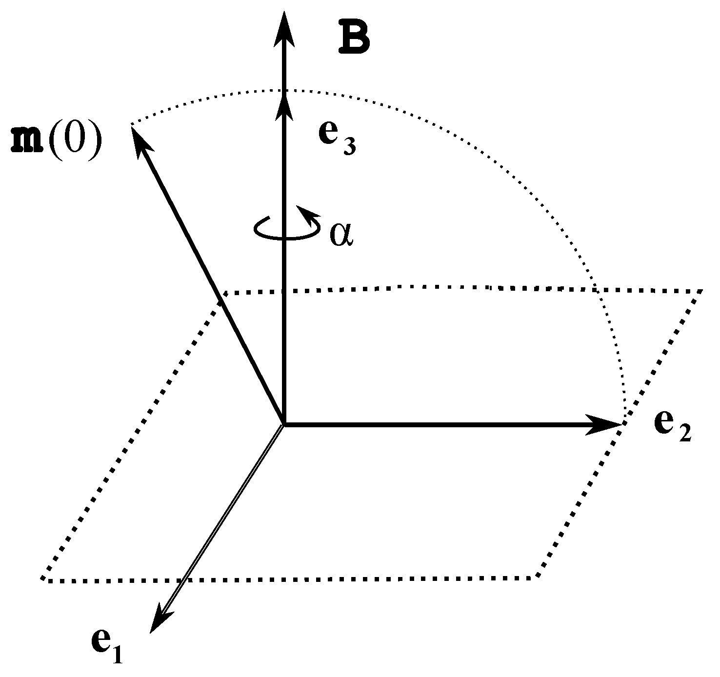
Figure 2.
Choice of Laboratory system for analysis of a charged symmetrical body.
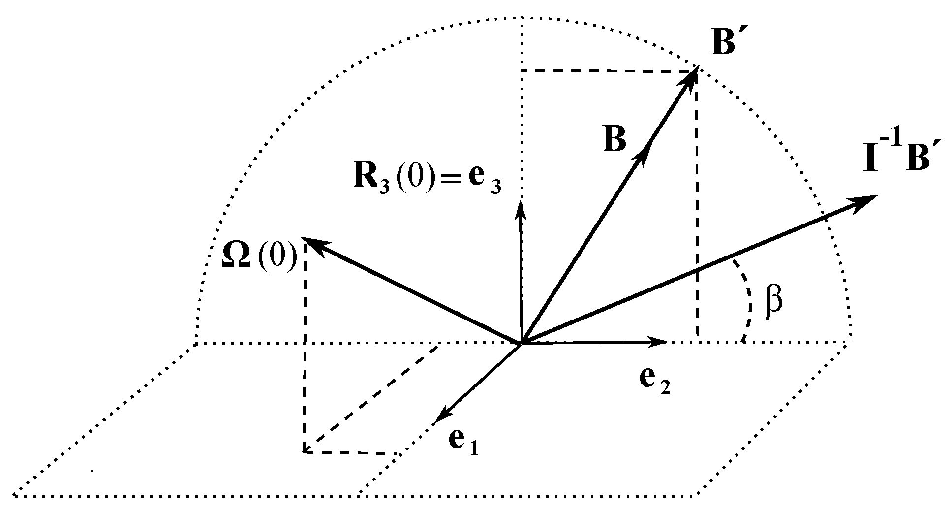
Figure 3.
The third components of initial data vectors , lying on drawn hyperboloids, turn out to be solutions to the equation of cubic pseudo-oscillator (47). Figure (a) shows the upper sheet of the hyperboloid of a short solenoid. Figure (b) shows the hyperboloid of a long solenoid. All drawn vectors and line segments lie in the plane of paper sheet. The basis vector is orthogonal to the plane of paper sheet and is not shown in the figure.
Disclaimer/Publisher’s Note: The statements, opinions and data contained in all publications are solely those of the individual author(s) and contributor(s) and not of MDPI and/or the editor(s). MDPI and/or the editor(s) disclaim responsibility for any injury to people or property resulting from any ideas, methods, instructions or products referred to in the content. |
© 2024 by the authors. Licensee MDPI, Basel, Switzerland. This article is an open access article distributed under the terms and conditions of the Creative Commons Attribution (CC BY) license (http://creativecommons.org/licenses/by/4.0/).
Copyright: This open access article is published under a Creative Commons CC BY 4.0 license, which permit the free download, distribution, and reuse, provided that the author and preprint are cited in any reuse.


