Submitted:
20 March 2024
Posted:
21 March 2024
You are already at the latest version
Abstract
In recent years, Global Navigation Satellite System reflectometry (GNSS-R) has been explored as a methodology for inland water body characterization. However, thorough characterization of the sensitivity and behavior of the GNSS-R signal to inland water bodies is still needed to progress this area of research. In this paper, we characterize the uncertainty associated with Cyclone Global Navigation Satellite System (CYGNSS) measurements on the determination of river width. The characterization study uses simulated data from a forward model that accurately simulates CYGNSS observations of mixed water/land scenes. The accuracy of the forward model is demonstrated by comparisons to actual observations of known water body shapes made at particular measurement geometries. Simulated CYGNSS data is generated over a range of synthetic scenes modeling a straight river subreach, and the results are analyzed to determine a predictive relationship between the peak SNR measured over the river subreaches and the river widths. An uncertainty analysis conducted using the predictive relationship indicates that for simplistic river scenes, the SNR over the river is predictive of the river width to within +/-5m. The presence of clutter (surrounding water bodies) within ~500m of the river causes perturbations in the SNR measured over the river that can render the river width retrievals unreliable. The results of this study indicate that under idealized conditions, GNSS-R data is able to measure river widths as narrow as 160m with high accuracy.
Keywords:
Riverine remote sensing
; GNSS Reflectometry
; CYGNSS
; flood prediction
; Water masks
1. Introduction
Global Navigation Satellite System reflectometry (GNSS-R) is an active field of research stemming from the success of several recent GNSS-R missions, including the TechDemoSat-1 (TDS-1) satellite [1], the Cyclone Global Navigation Satellite System (CYGNSS) mission [2], and the Chinese BuFeng-1 A/B twin satellites [3]. Unlike traditional imagers, GNSS-R allows for constellations of low-cost receivers that collect bistatic radar data scattering off the Earth’s surface through vegetation canopies and in all weather conditions including clouds and rain. The bistatic radar data contains signatures that have been used for wide-ranging Earth Science applications, including measuring ocean surface wind speeds [4], soil moisture [5,6,7], inland water body mapping [8,9,10,11,12,13,14,15], and river width [16] and surface slope [17] estimation.
This paper explores the potential for using GNSS-R to measure river width, a currently under-sampled parameter. River width is a valuable hydrology metric because of its correlation to river discharge (and therefore of use for flood monitoring, prediction, and water resources management) as well as its necessity as an input parameter to hydraulic routing and distributed hydrology models. These models are used to predict other hydrological quantities on the watershed-scale such as inundation, sediment transport, and soil saturation. Currently, river width data is typically only available for large-scale regions using long-term records of satellite imagery. Databases such as the Global Width Database for Large Rivers [18], and the North American River Width (NARWidth) data set [19] rely on long-term imagery records from the SRTM and Landsat missions, respectively, to represent river extents at mean flow conditions. These databases provide large-scale data that are useful for climatological studies but do not capture the dynamic range of rivers. This limits their utility for flood monitoring and other applications requiring accurate, up-to-date riverine extents. The Surface Water and Ocean Topography (SWOT) mission, launched by NASA in December 2022, aims to address the river width data scarcity with its innovative remote sensing instrument, the Ka-band Radar Interferometer (KaRIn), that will provide global measurements of rivers that are at least 100 meters wide [20]. The SWOT mission should lead to unprecedented global surveillance of the Earth’s rivers; however, its revisit rate will be on the order of weeks, which is still limiting for rapidly changing, high-risk events. Conversely, data from GNSS-R, which could provide riverine monitoring with revisit rates on the order of hours to days because of the low cost of GNSS-R receivers and the ability to launch constellations of instruments, has the potential to supplement and provide independent validation of the SWOT river width data.
To investigate this potential, in this paper we analyze simulated, high temporal resolution CYGNSS data to answer previously unaddressed questions about the feasibility of using GNSS-R signals to measure changes in river width by characterizing the signal's sensitivity to river width, satellite geometry, and scene complexity. The use of simulated data allows us to isolate and vary individual parameters impacting the signal (e.g., the width and shape of the river, the approach angle of the track with respect to the river's orientation), while controlling for parameters that vary from overpass to overpass (e.g., satellite geometry, land surface conditions). The synthetic processed CYGNSS raw IF data is generated with an End-to-End Simulator (E2ES), using geometry from actual CYGNSS overpasses that span low to high incidence angles in order to analyze the incidence angle's impact on the signal's sensitivity to river width.
Section 2 of this paper reviews the E2ES used to generate the simulated CYGNSS data used in this study and validates the accuracy of the simulations with comparisons to observations made by CYGNSS. Section 3 describes the experimental design approach taken and the set of simulations that were created to perform the analysis. Section 4 presents the results of the analysis, and Section 5 includes a discussion of the results. Section 6 concludes with a summary and recommendations.
2. End to End Simulator
2.1. Model Description
The GNSS signal reflected from inland scenes is comprised of forward scatter from smooth (e.g., inland water bodies) and rough (e.g., land) surfaces. The scattering properties over these two surface types are very different, with the forward scattering received from smooth surfaces typically orders of magnitude stronger than that from rough surfaces. The significant increase in signal strength over smooth surfaces vs. rough land is the reason that GNSS-R data is highly sensitive to the presence and size of inland water bodies. An end-to-end simulator (E2ES) has been developed that accurately simulates the overland CYGNSS signal by combining two models that calculate the relative contribution of incoherent and coherent scattering at the specular point (SP) of reflection from the distribution of rough and smooth surfaces, respectively. The incoherent scattering model is derived from a previously developed E2ES which was used for simulating the CYGNSS incoherent scattering signal over a rough surface such as the ocean [21], and is based on the bistatic radar equation [22]:
where is the simulated signal-to-noise ratio (SNR) of the incoherent scattering signal component, ( represents the delay, Doppler coordinates in the delay Doppler map (DDM), is the GNSS transmitted power, and are the receiver and transmitter antenna gains, is the lag correlation function due to the correlation of the scattered signal with a local replica of the GPS pseudorandom noise (PRN) code, is the Doppler filter response due to selective filtering of the Doppler-shifted received signal, and are the distances from the SP to the transmitter and the receiver, respectively, and is the signal wavelength (19 cm). The integral is performed over a region of the surface centered on the specular reflection point (SP) and extending out until and are sufficiently small.
The coherent scattering model is based on the Huygens-Kirchhoff principle, which is a statistical model for coherently reflected signals from an irregular surface [23]. For a single SP track measurement, a simplified version of the Huygens-Kirchhoff statistical model is given by the Friis equation:
where is the SNR of the coherently scattered signal, is the complex Fresnel reflection coefficient of the smooth surface, is the wavenumber, is the RMS height of the rough surface, is the fraction of the First Fresnel Zone (FFZ) that contains water, and is the incidence angle.
To reproduce the CYGNSS measurements along a SP track, the combined coherent+incoherent E2ES requires input of the time varying measurement geometry for signal propagation from the GPS to the CYGNSS satellite along the specular reflection path. A water mask is also input that defines which cells of the computational grid contain water and land [23]. Additionally, the incoherent and coherent scattering components of the model output must each be scaled by an appropriate calibration term to match the scale factor of the CYGNSS measurements that results from its receiver gain, which is also time varying (mostly due to the temperature dependence of the receiver gain). These calibration terms are determined empirically for each track by comparing E2ES outputs to CYGNSS observations over segments of the track believed to be purely coherent and purely incoherent. This process is described below in the Validation section.
It should be noted that the E2ES makes several assumptions about the properties of the surface. The water surface is assumed to be perfectly smooth (i.e., in Equation (2)) and a constant NBRCS value of is assumed over land. Additionally, the water surface is assumed to have a Fresnel reflection coefficient, , of 1. These assumptions will affect the relative magnitudes of the SNR over land and water, but do not significantly impact the width of the water portion of the SNR track that is used to determine river width. Statistically representative noise is added to the simulated SNR with a Gaussian, zero-mean distribution. The standard deviation of the noise is estimated using a SP track over Lake Ilopango that was used for an E2ES validation study in [23]. The resulting noise model is
where is the standard deviation of the additive noise in the SNR, is the incoherent averaging time in seconds, and is the average SNR over the SP track.
2.2. Validation
The ability of the E2ES to properly simulate the behavior of CYGNSS observations in mixed coherent+incoherent conditions was demonstrated in [23] by a comparison between observed and simulated measurements of a CYGNSS track that crossed directly over a large lake (Lake Ilopango in El Salvador). The comparison focused on measurements near the land/water boundary, where the scattering transitions from purely incoherent to purely coherent conditions occur. Lake Ilopango is much larger than the FFZ of the coherent scattering component, so there is a single transition zone at the shoreline where the measurements contain a mixture of both coherent and incoherent scattered signals. In the study conducted here, we consider more complicated inland water body scenarios whereby multiple water bodies may be present and each of them may be smaller than the FFZ. This can result in a broader region over which both types of scattering are present, and a more complicated measurement response as small land and water surfaces pass in and out of the first and higher order Fresnel zones [24]. For this reason, we consider here additional E2ES validation for comparisons between simulated and observed measurements of more complicated scenes.
The validation cases are shown in Figure 1 for raw IF data collections made over the Río Santiago in Peru on 17 Mar 2022 (top row), a more recent overpass of Lake Ilopango in El Salvador than that considered in [23], on 8 Oct 2023, which skims the edge of the waterbody (middle row), and the Roosevelt River in Brazil on 26 Mar 2022 (bottom row). The figures in the left column show the simulated SNR from the E2ES (dashed red lines) plotted vs. SP track distance along with the processed CYGNSS raw IF observations (solid blue lines). The right column shows the georeferenced SP track on the Earth’s surface relative to Google Earth imagery of the water bodies (colored line), where the line color is proportional to the observed SNR magnitude. The water mask used in each simulation is overlaid on the maps in dark blue. The water mask for each of these simulations is derived from Landsat or Google Earth imagery using a simple land/water classifier. The raw IF processing of the CYGNSS observations was conducted with 1 ms coherent integration and 50 ms incoherent averaging and computed in 1 ms time steps. Incoherent averaging of the simulated signal was conducted over a 50 ms window to match the processed CYGNSS raw IF data. Noise was added using the empirical noise model in Equation (3).
The coherent and incoherent calibration terms for each of these simulations are derived by scaling the E2ES output to the observations in the following manner. First, representative values of the mean incoherent scattering and the peak coherent scattering are calculated from the processed CYGNSS raw IF data. For each SNR time series, a histogram is created from the SNR values. The 10th percentile value is used to define the incoherent scattering reference value. For the coherent scattering reference value, two possibilities exist: in cases where there is a single, clearly defined peak in the observed SNR, the maximum SNR defines the coherent scattering reference value. In cases where the SNR plateaus or otherwise does not have a clearly defined peak value, the 99th percentile value is defined as the reference coherent scattering value. Because of the noise in the data and the influence from nearby water bodies, we have found this approach to be more accurate than taking averages or maxima/minima over the time series to calculate the representative values for the observed data. Next, reference values for the output of the coherent and incoherent scattering models are calculated in a similar manner. The coherent and incoherent calibration terms are then calculated by taking the ratio of the representative coherent and incoherent scattering values to those obtained directly from the observations. The individual simulation components are then scaled by their respective calibration terms prior to summing the components and adding simulated noise. Table 1 shows the values used in this process for the three tracks shown in Figure 1.
The overall shape and magnitude of the simulated SNR series in Figure 1 match the observations well. For the river cases (top and bottom row of Figure 1), the peak and shape of the waveform corresponding to the rivers match closely. In the Lake Ilopango case (middle row of Figure 1), the SP track grazes the boundary of the water body rather that passing across its center, leading to a lower magnitude waveform that spans several kilometers. Overall, the results in Figure 1 indicate that given a reasonably accurate water mask, the E2ES captures the main features of the CYGNSS raw IF observations as well as much of the fine structure in the vicinity of the land/water transition region. In the following section, we use the E2ES as a tool to examine CYGNSS sensitivity a number of to river properties.
3. Experimental Design
We consider three properties of the GNSS-R SNR signal during a river overpass that contain information about riverine properties. The first is the waveform width during the river overpass, which in a previous work [16] was determined to be correlated with observed streamflow. The second property, explored in this work, is the SNR value itself at the center of the river overpass. In cases where the river width is sufficiently narrow that , changes in the SNR value will be correlated with changes in river width and therefore this approach can resolve the width of small rivers. A third property is the impact on the SNR measured at the center of the river overpass due to other nearby water bodies.
The goal of this study is to examine the relationship between the CYGNSS SNR measured over the river crossing and the river width, and to determine the sensitivity of the relationship to measurement geometry, river width, and surrounding clutter. To assess the measurement geometry impact, the SP track’s incidence angle and its approach angle relative to the river orientation are varied. To assess the impact of the river’s width, overpasses of rivers with widths of 160m, 176m, and 192m are simulated. To assess the impact of nearby clutter on the SNR over the river, we examine the impact of a large lake on the signal as a function of its distance from the river.
To assess the impact of incidence angle, simulations are generated using three different CYGNSS overpasses with varying incidence angles. The three tracks were selected to occur over very large water bodies to facilitate the determination of the calibration terms. The exact extent of the water bodies at the time of the CYGNSS data collection is not known but, by choosing overpasses of very large water bodies, the can safely be assumed to be 1 when the SP track is near the center of the water body. The observations and simulations are shown in Figure 2 for Lake Ilopango in El Salvador (top), a large reservoir created by the UHE Rondon II hydroelectric power plant in Brazil (middle), and the Marañón River in Peru (bottom). E2ES outputs were calibrated as described in the Validation section above. Note that for the Marañón River, few Landsat images were available for this location. A comparison of the observed and simulated SNR indicates that the mask that was selected, which was based on the best available Landsat image, underrepresents the true extent of the river at the time of the CYGNSS raw IF data collection. Despite the significant discrepancies along the water/land transitions for the Marañón River, and to a lesser degree for the Lake Ilopango and UHE Rondon II overpasses, the signals match well over the plateau section of the SP track where the signal is saturated by coherent scattering (i.e., ). This is the portion of the signal that is used to determine the coherent scattering calibration term. Table 2 lists the calibration terms for the three tracks shown in Figure 2 along with other relevant measurement parameters for the three input geometry files. The simulations were run with same E2ES parameters used for the Validation cases.
4. Results
4.1. River Width Estimation from Peak SNR
The first cases considered examine the relationship between river width and the peak SNR value over the river for scenes with an isolated, straight river and in which the SP track is perpendicular to the river. These cases provide the simplest scenario, and the SNR waveforms have a single peak value that occurs when the SP is at the river centerline. Figure 3 shows the results of these simulations: the SNR along the SP track is shown for river widths of 160m, 176m, and 192m (blue, green, and red lines on the top row of figures) for each of the three tracks. The bottom row of the figure shows the water masks used for each river width: w = 160m (bottom left), w = 176m (bottom middle), and w = 192m (bottom right). Note that in these simulations, no simulated noise is added. By examining the relationship between the peak SNR that is measured over the river centerline and the river width in each case, a model can be derived that predicts the river width from the SNR peak value (Figure 4). The model has the form:
where is the predicted river width, and are constants determined by the regression, and is the SNR in linear units as measured when the SP point is at the river centerline. The regression constants and vary for each incidence angle and are shown in Table 3.
The isolated, straight river analysis is repeated for a set of cases where the SP track makes an oblique (45-degree) approach angle with respect to the river centerline. The results from these simulations are shown in Figure 5, which is analogous to Figure 3. Qualitatively, the waveforms corresponding to the same incidence angles and river widths have lower amplitudes as compared to the perpendicular approach angles (top row of Figure 3 vs. Figure 5). Note that the waveforms at the 45-degree approach angle are wider compared to the perpendicular approach angle cases for the same incidence angles and river widths. The reduction in peak SNR and expansion of the waveform width increases with increasing incidence angle (Figure 5, top row). These behaviors can be explained by considering the for the perpendicular vs. 45-degree approach angle cases, where the ellipse encompassing the FFZ along the SP track for the perpendicular crossing cases does not contain water until the SP point is ~600m, ~680m, and ~710m from the river center point for the 14 degree, 31 degree, and 42 degree incidence angles, respectively. When the major axis of the FFZ ellipse is aligned at a 45-degree angle to the river centerline, a portion of the river is encompassed by the FFZ earlier in the SP track, and this is reflected in the start of the waveform rising edge at ~800, ~1000m, and ~2000m for the 14 degree, 31 degree, and 42 degree incidence angles, respectively. The shape of the FFZ ellipse elongates with increasing incidence angle, so when the incidence angle is larger the waveform appears more spread out.
4.2. Error Analysis
The precision of the river width estimates is a function of measurement noise and can be determined by a propagation of errors analysis. The resulting standard deviation of , , given the standard deviation of SNR, , is derived from Equation (4) by
Values of for each river width and measurement geometry are shown in Table 5 and Table 6 for perpendicular and oblique approach angles, respectively. Note that the precision is fairly independent of river width but increases significantly as incidence angle decreases. Overall, the small uncertainty values of 3-5 m are a result of the very high SNR values for coherently scattered signals and the linear dependence of SNR on , which varies directly with river width for narrow rivers. A comparison of Table 5 and Table 6 shows that the precision is comparable for the perpendicular and oblique approach angle cases and is on the order of 4% or less for the perpendicular approach angle cases, and 3% or less for the oblique approach angle cases.
While precision characterizes the dependence of the river width estimation error on measurement noise, the accuracy of the estimator characterizes how well the retrieval algorithm performs without noise and is calculated as the root mean square (RMS) difference between the true river width and the width predicted by the SNR-based models, i.e., the residual error in the regressions shown in Figure 4 and Figure 6:
where are the true river widths (160, 176, and 192m), and are the estimated river widths from the models. The accuracy errors for each track and incidence angle are shown in Table 7. The accuracy errors for the oblique approach angle cases are an order of magnitude smaller than those for the perpendicular cases and range from 3-68cm.
The total uncertainty in the retrieval estimates is the root sum square of the precision and accuracy:
Applying Equation (7) to the largest values of precision error for each track, an upper bound on the total uncertainty in the width retrieval estimate is calculated for the perpendicular and oblique approach angle cases (Table 8). The total uncertainties range from ~3-5m.
4.3. Impact of Clutter on River Width Prediction from Peak SNR
For the isolated river cases examined above, the SNR peak of each SP track coincides with the SP track center point over the river, and its magnitude increases in proportion to the river width. When nearby water bodies (clutter) are present, their scattered signals will be combined with the scattering from the river itself. Due to the extended region of sensitivity to scattering in the first and higher order Fresnel zones, it can be expected that when the clutter is close enough to the river, scattering from it will begin to perturb the SNR peak and cause the predictive relationship described by Equation (4) to break down. To characterize the impact of clutter on the SNR waveform, simulations are conducted in which a circular lake with a 1000m diameter is located on the western side of the river at varying radial distances as measured from the center point of the SP track crossing over the river to the center point of the lake. The perturbations in the SNR peak measured at the center of the river are determined for each SP track and river width. The perpendicular SP tracks are considered in Figure 7 and the oblique SP tracks in Figure 8. The perturbations are then compared to the standard deviation of the noise in the SNR measurements. When the perturbation exceeds the noise, it is considered significant, and the clutter is considered too close to the river.
The results in Figure 7 indicate that clutter becomes problematic for the perpendicular SP track crossing at ~850m for the low incidence angles (Track 1). This corresponds to a distance of ~350m from the SP track over the river and the edge of the lake. For the higher incidence angles (Tracks 2 and 3) the lake can pose a problem when located as far as ~1400m away (~900m from the edge of the clutter water body). For the oblique approach angle cases (Figure 8), the lake becomes problematic when it is centered ~1000m from the river center point for all incidence angles and river widths (~500m from the edge of the clutter water body).
Because of the non-linear behavior of the SNR peak with respect to the lake distance and the finite number of simulations run, the exact distance of the lake from the river SP crossing where the SNR perturbation becomes significant cannot be determined by these simulations, but these results indicate that clutter from large (on the order of 1km wide) water bodies located within 500m of a river can introduce perturbations in the peak SNR at river center, while large water bodies located > ~900m from the river do not significantly impact the peak SNR related to the river crossing.
5. Discussion
The ability of GNSS-R measurements to resolve the width of rivers during their specular point river crossings has been expanded from previous work, in which the width of the waveform corresponding to a river overpass was correlated to the observed streamflow [16]. In the present work, we investigate the information contained in the SNR values for determining the width of narrow (< 200 m) rivers. We find that the decreased strength of the scattered signal itself, due to the fraction of the first Fresnel zone that contains water being < 1, contains useful information about river width because it scales linearly with the . The fraction reaches a peak value when the specular point is located at the center of the river, and hence the and SNR peak are both highly correlated with the river width.
Using the relationship between river width and SNR peak for narrow rivers, a parametric model is derived. The functional form of the model is found to be robust to variations in measurement geometry (in particular, the incidence angle of the specular reflection) and to the approach angle of the specular point track relative the river. However, the parameter values in the model vary with both of these conditions. For the case of incidence angle variations, the parameters vary because the size of the first Fresnel zone also varies with incidence angle. For the case of the approach angle variations, the parameters vary because the alignment of the major and minor axes of the first Fresnel zone relative to the river vary, thereby affecting the fraction that is filled by water for a given river width.
The sensitivity of river width estimates made from the SNR peak to noise in the SNR measurements is also examined by propagating the measurement noise through the parametric model. The river width uncertainty ranges between 3 and 5 m for river widths of 160-190 m, or roughly 2-3%. The high precision is a result of the very high SNR measurements that typically result from coherent scattering surface such as rivers and lakes.
The clutter effect from nearby water bodies is also examined, by introducing an artificial lake in the simulated water mask and varying its distance from the river. It is found that the SNR peak at the center of the river begins to be perturbed when the center of the lake is ~1.5 km away from the river (~1 km from the center of the river to the edge of the lake) and the perturbation becomes significant (i.e., becomes greater than the standard deviation of the measurement noise) when the lake is within ~1.0 km of the river (~500m from the center of the river to the edge of the lake). While this result is found using a somewhat idealized simulation, it is consistent with the size of the first Fresnel zone and can be considered a useful general guideline for identifying when the presence of nearby waterbodies should be considered significant clutter.
Due to the limited number of simulations analyzed in this work and the infinite number of possibilities for river shape, orientation relative to SP track, measurement geometry, and surrounding clutter, the uncertainty in river width predicted from GNSS-R measurements that is calculated in this work cannot be generalized to river conditions far different from those considered here. It is possible, for example, that when the over a river becomes sufficiently large or small, the relationships determined in this work may no longer hold. Additionally, the complexity of the interaction between higher order Fresnel zones in the presence of clutter or a meandering river shape can be expected to alter the relationships determined in the simulated cases considered above. Further research is needed to better understand the impact of these complexities on the uncertainties associated with the use of GNSS-R SNR to predict river width and to refine the predicted uncertainty.
6. Conclusions
In this work, the ability of GNSS-R bistatic radar SNR data to measure the width of narrow rivers was assessed. The theoretical basis for the GNSS-R SNR sensitivity to river width derives from the vastly differing properties of the scattering received by a GNSS-R receiver over smooth (coherent scattering) vs. rough (incoherent scattering) surfaces. An End-to-End Simulator has been used to accurately simulate these two scattering modalities over scenes that contain both water (smooth surfaces) and land (rough surfaces) and create synthetic data that allows for controlled study of factors impacting the GNSS-R SNR over rivers. The output of the E2ES is the combined signal from the coherent and incoherently scattering components over a simulated section of SP track. The E2ES is validated for SP tracks over small inland water bodies, where the first Fresnel zone fraction is < 1 over the entirety of the track, and is shown to reproduce the CYGNSS observations well.
Simulated CYGNSS data for straight rivers ranging from 160-192m in width were analyzed for both perpendicular SP track river overpasses and those made at a 45-degree approach angle with respect to the river orientation. Three CYGNSS overpasses were selected for the generation of the simulated data that span low (14 degree), mid-range (31 degree), and higher (42 degree) incidence angles to assess the width retrieval capability as a function of the measurement geometry. Predictive models of the river width as a function of the SNR measured directly over the river were determined from numerical regressions, and the width was found in all cases to vary proportionally as , where the value of ranges from ~0.5-0.6 and decreases with increasing incidence angle.
An error analysis was performed that assessed the width retrieval error in terms of both precision and accuracy. Total uncertainty was found to range from ~2-5m, with uncertainty decreasing with increasing incidence angle.
Simulations were also conducted with clutter in the form of a large circular lake located in the vicinity of the river. The distance at which the impact of the lake on the SNR magnitude over the river becomes significant was identified as ~500m from the center of the river to the edge of the lake. This finding is consistent with the distance where the lake would begin to enter the FFZ for a SP over the river.
In summary, a robust modeling approach has been determined that allows river width to be estimated with ~5 m uncertainty when clutter does not exist within ~500m of the river. Further research is needed to determine the limits on the river width retrieval from GNSS-R SNR data over rivers and to examine the impact of factors that are not fully characterized in the simulated data used herein.
Funding
This research was funded by the National Aeronautics and Space Administration Earth Science Division (80NSSC21K1119).
Data Availability Statement
CYGNSS data used during this study is available from the NASA Physical Oceanography Distributed Active Archive Center (PODAAC) at https://podaac.jpl.nasa.gov/CYGNSS?tab=mission-objectives§ions=about%2Bdata. The coherent+incoherent E2ES code and generated synthetic data is available upon request; please contact the corresponding author.
Acknowledgments
This research is supported by the National Aeronautics and Space Administration under Grant No. 80NSSC21K1119 issued through the Earth Science Division Science Mission Directorate. The authors would like to thank the ESA Network of Resources Initiative for providing Sentinel-2 data used in this project.
Conflicts of Interest
The authors declare no conflicts of interest.
References
- Foti, G.; Gommenginger, C.; Jales, P.; Unwin, M.; Shaw, A.; Robertson, C.; Roselló, J. Spaceborne GNSS reflectometry for ocean winds: First results from the UK TechDemoSat-1 mission. Geophys. Res. Lett. 2015, 42, 5435–5441. [Google Scholar] [CrossRef]
- Ruf, C.; Unwin, M.; Dickinson, J.; Rose, R.; Rose, D.; Vincent, M.; Lyons, A. CYGNSS: Enabling the Future of Hurricane Prediction [Remote Sensing Satellites]. IEEE Geosci. Remote. Sens. Mag. 2013, 1, 52–67. [Google Scholar] [CrossRef]
- Jing, C.; Niu, X.; Duan, C.; Lu, F.; Di, G.; Yang, X. Sea Surface Wind Speed Retrieval from the First Chinese GNSS-R Mission: Technique and Preliminary Results. Remote. Sens. 2019, 11, 3013. [Google Scholar] [CrossRef]
- Ruf, C.S.; Gleason, S.; McKague, D.S. Assessment of CYGNSS Wind Speed Retrieval Uncertainty. IEEE J. Sel. Top. Appl. Earth Obs. Remote Sens. 2018, 12, 87–97. [Google Scholar] [CrossRef]
- Chew, C.C.; Small, E.E. Soil Moisture Sensing Using Spaceborne GNSS Reflections: Comparison of CYGNSS Reflectivity to SMAP Soil Moisture. Geophys. Res. Lett. 2018, 45, 4049–4057. [Google Scholar] [CrossRef]
- Al-Khaldi, M.M.; Johnson, J.T.; O'Brien, A.J.; Balenzano, A.; Mattia, F. Time-Series Retrieval of Soil Moisture Using CYGNSS. IEEE Trans. Geosci. Remote. Sens. 2019, 57, 4322–4331. [Google Scholar] [CrossRef]
- Clarizia, M.P.; Pierdicca, N.; Costantini, F.; Floury, N. Analysis of CYGNSS Data for Soil Moisture Retrieval. IEEE J. Sel. Top. Appl. Earth Obs. Remote. Sens. 2019, 12, 2227–2235. [Google Scholar] [CrossRef]
- Gerlein-Safdi, C.; Ruf, C.S. A CYGNSS-Based Algorithm for the Detection of Inland Waterbodies. Geophys. Res. Lett. 2019, 46, 12065–12072. [Google Scholar] [CrossRef]
- Chew, C.; Small, E. Estimating inundation extent using CYGNSS data: A conceptual modeling study. Remote. Sens. Environ. 2020, 246, 111869. [Google Scholar] [CrossRef]
- Al-Khaldi, M.M.; Johnson, J.T.; Gleason, S.; Chew, C.C.; Gerlein-Safdi, C.; Shah, R.; Zuffada, C. Inland Water Body Mapping Using CYGNSS Coherence Detection. IEEE Trans. Geosci. Remote. Sens. 2021, 59, 7385–7394. [Google Scholar] [CrossRef]
- Al-Khaldi, M.M.; Johnson, J.T.; Gleason, S.; Loria, E.; O'Brien, A.J.; Yi, Y. An Algorithm for Detecting Coherence in Cyclone Global Navigation Satellite System Mission Level-1 Delay-Doppler Maps. IEEE Trans. Geosci. Remote. Sens. 2021, 59, 4454–4463. [Google Scholar] [CrossRef]
- Gerlein-Safdi, C.; Bloom, A.A.; Plant, G.; Kort, E.A.; Ruf, C.S. Improving Representation of Tropical Wetland Methane Emissions With CYGNSS Inundation Maps. Glob. Biogeochem. Cycles 2021, 35, e2020GB006890. [Google Scholar] [CrossRef]
- Ghasemigoudarzi, P.; Huang, W.; De Silva, O.; Yan, Q.; Power, D. A Machine Learning Method for Inland Water Detection Using CYGNSS Data. IEEE Geosci. Remote. Sens. Lett. 2022, 19, 1–5. [Google Scholar] [CrossRef]
- Rodriguez-Alvarez, N.; Munoz-Martin, J.F.; Morris, M. Latest Advances in the Global Navigation Satellite System—Reflectometry (GNSS-R) Field. Remote. Sens. 2023, 15, 2157. [Google Scholar] [CrossRef]
- Carreno-Luengo, H.; Ruf, C.S.; Gleason, S.; Russel, A. Detection of inland water bodies under dense biomass by CYGNSS. Remote. Sens. Environ. 2024, 301, 113896. [Google Scholar] [CrossRef]
- Warnock, A.; Ruf, C. Response to Variations in River Flowrate by a Spaceborne GNSS-R River Width Estimator. Remote. Sens. 2019, 11, 2450. [Google Scholar] [CrossRef]
- Wang, Y.; Morton, Y.J. River Slope Observation From Spaceborne GNSS-R Carrier Phase Measurements: A Case Study. IEEE Geosci. Remote. Sens. Lett. 2022, 19, 1–5. [Google Scholar] [CrossRef]
- Yamazaki, D.; O’Loughlin, F.; Trigg, M.A.; Miller, Z.F.; Pavelsky, T.M.; Bates, P.D. Development of the Global Width Database for Large Rivers. Water Resour. Res. 2014, 50, 3467–3480. [Google Scholar] [CrossRef]
- Allen, G.H.; Pavelsky, T.M. Patterns of river width and surface area revealed by the satellite-derived North American River Width data set. Geophys. Res. Lett. 2015, 42, 395–402. [Google Scholar] [CrossRef]
- Biancamaria, S.; Lettenmaier, D.P.; Pavelsky, T.M. The SWOT mission and its capabilities for land hydrology. In Remote Sensing and Water Resources; Cazenave, A., Champollion, N., Benveniste, J., Chen, J., Eds.; Springer Nature: Basel, Switzerland, 2016; pp. 117–147. ISBN 978-3-319-32448-7. [Google Scholar] [CrossRef]
- O’Brien, A., S. Gleason, J. Johnson, and C. Ruf (2014). The end-to-end simulator for the cyclone GNSS (CYGNSS) mission. IEEE Trans. Geosci. Remote Sens., vol. 3, no. 2, pp. 306–315, 2014.
- Balakhder, A.M.; Al-Khaldi, M.M.; Johnson, J.T. On the Coherency of Ocean and Land Surface Specular Scattering for GNSS-R and Signals of Opportunity Systems. IEEE Trans. Geosci. Remote. Sens. 2019, 57, 10426–10436. [Google Scholar] [CrossRef]
- Carreno-Luengo, H.; Warnock, A.; Ruf, C.S. The Cygnss Coherent End-to-End Simulator: Development and Results. IGARSS 2022 - 2022 IEEE International Geoscience and Remote Sensing Symposium. pp. 7441–7444.
- Camps, A. Spatial Resolution in GNSS-R Under Coherent Scattering. IEEE Geosci. Remote. Sens. Lett. 2020, 17, 32–36. [Google Scholar] [CrossRef]
Figure 1.
E2ES results compared to CYGNSS raw IF observations for three water bodies. The left column shows the processed CYGNSS raw IF SNR (solid blue lines) and the E2ES simulated SNR (dashed red lines). The right column shows the SP track overpass of each water body, colored by the CYGNSS SNR. Top row: Overpass of the Rio Santiago in Peru on 17 Mar 2022; Middle row: Overpass grazing Lake Ilopango in El Salvador on 8 Oct 2023; Bottom row: Overpass of the Roosevelt River in Brazil on 26 Mar 2022.
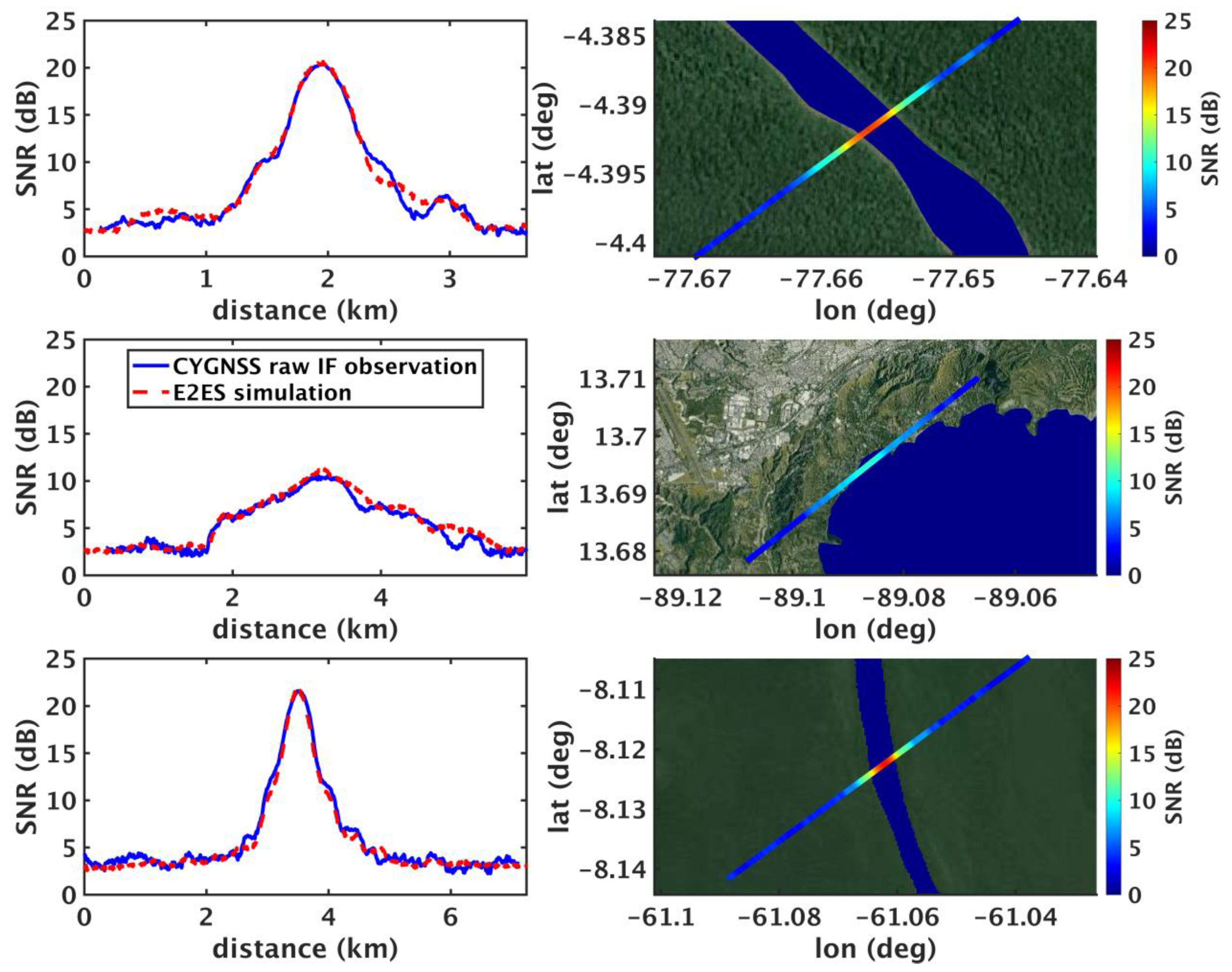
Figure 2.
CYGNSS raw IF overpasses used as input for the synthetically generated river simulations. Top: Overpass of Lake Ilopango in El Salvador on 22 Aug 2019; Middle: Overpass of the reservoir near the UHE Rondon II hydroelectric power plant in Brazil on 7 Jul 2022; Bottom: Overpass of the Marañón River in Peru on 24 Oct 2022. The left figures show comparisons of the simulated E2ES SNR (red dashed lines) and the observations (solid blue lines). Right figures show the SP track, colored by observed SNR, relative to the water masks used for each simulation (blue).
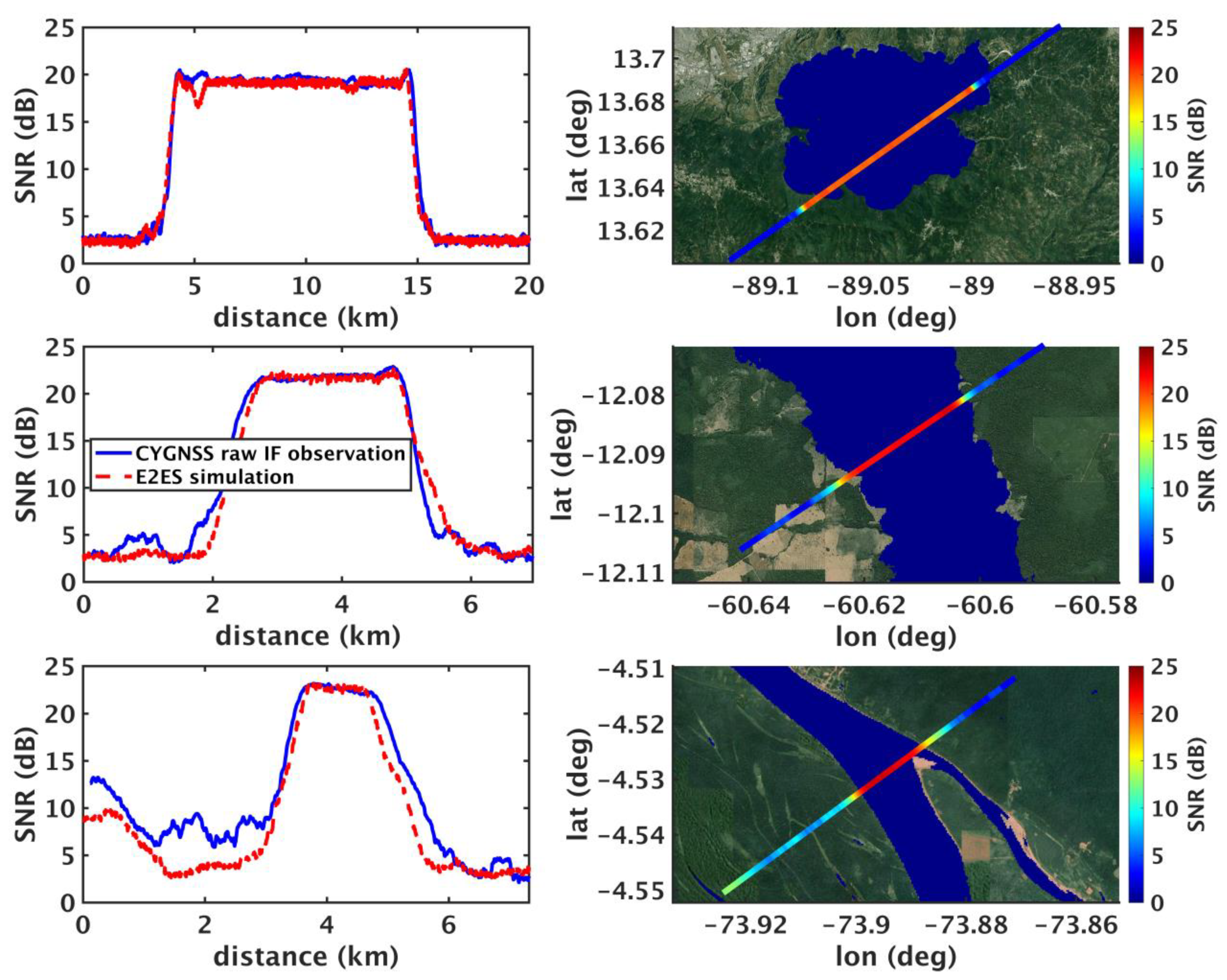
Figure 3.
Simulations of straight river overpasses where the SP track makes a perpendicular (angle = 90 degrees) approach angle relative to the river orientation, for Track 1 (left column), Track 2 (middle column), and Track 3 (right column). Top row shows the simulated SNR for river widths of 160m (blue lines), 176m (green lines), and 192m (red lines), corresponding to the input masks shown in the bottom row, where the river is shown as the blue line and SP tracks as shown as the black arrowed lines.
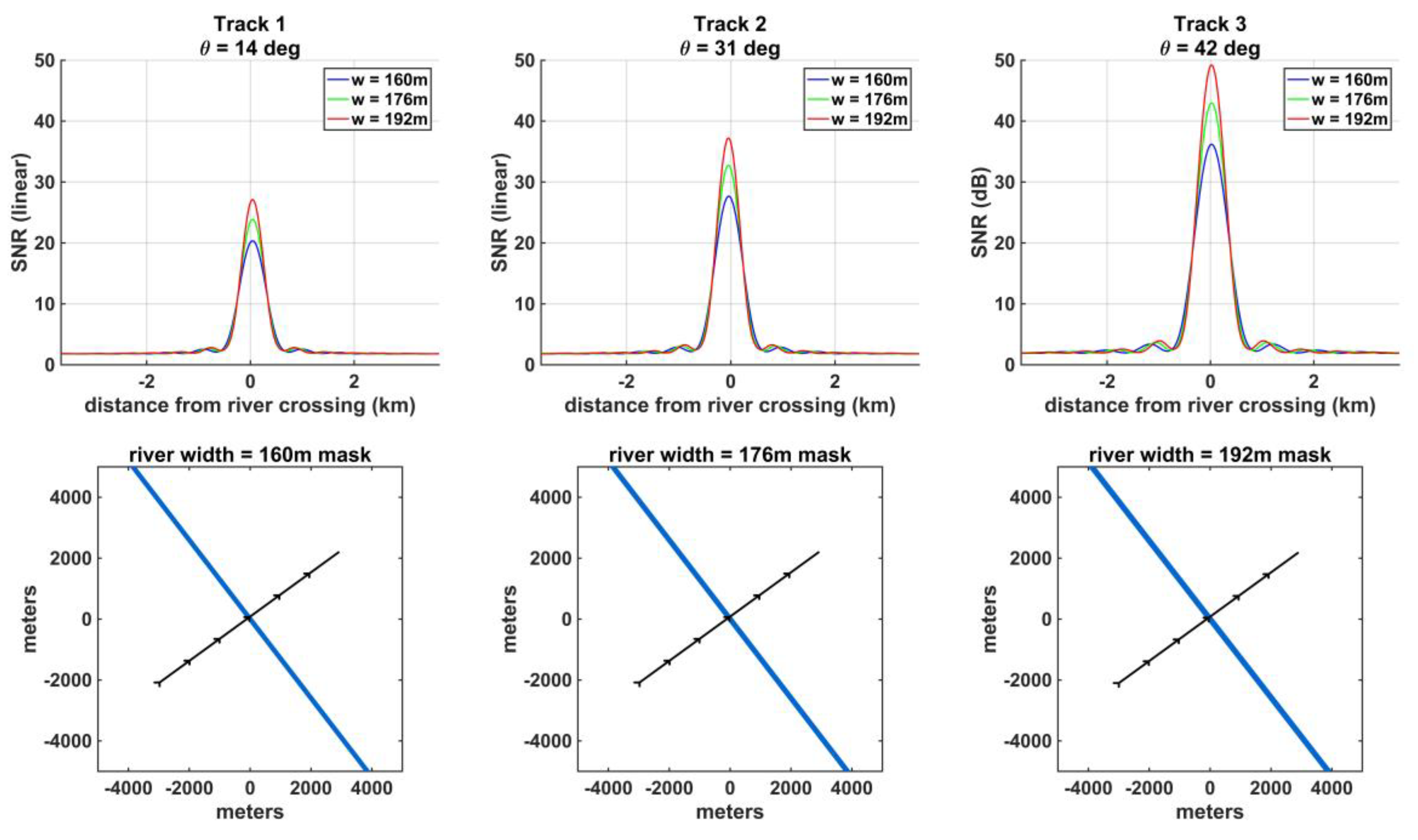
Figure 4.
SNR peak data points vs. river width (dots) and best fit regression (solid lines) for Track 1 (blue), Track 2 (green), and Track 3 (red) for the perpendicular SP track crossings of a straight, isolated river.
Figure 4.
SNR peak data points vs. river width (dots) and best fit regression (solid lines) for Track 1 (blue), Track 2 (green), and Track 3 (red) for the perpendicular SP track crossings of a straight, isolated river.

Figure 5.
Simulations of straight river overpasses where the SP track makes an oblique (angle = 45 degrees) approach angle relative to the river orientation, for Track 1 (left column), Track 2 (middle column), and Track 3 (right column). Top row shows the simulated SNR for river widths of 160m (blue lines), 176m (green lines), and 192m (red lines), corresponding to the input masks shown in the bottom row, where the river is shown as the blue line and SP tracks as shown as the black arrowed lines.
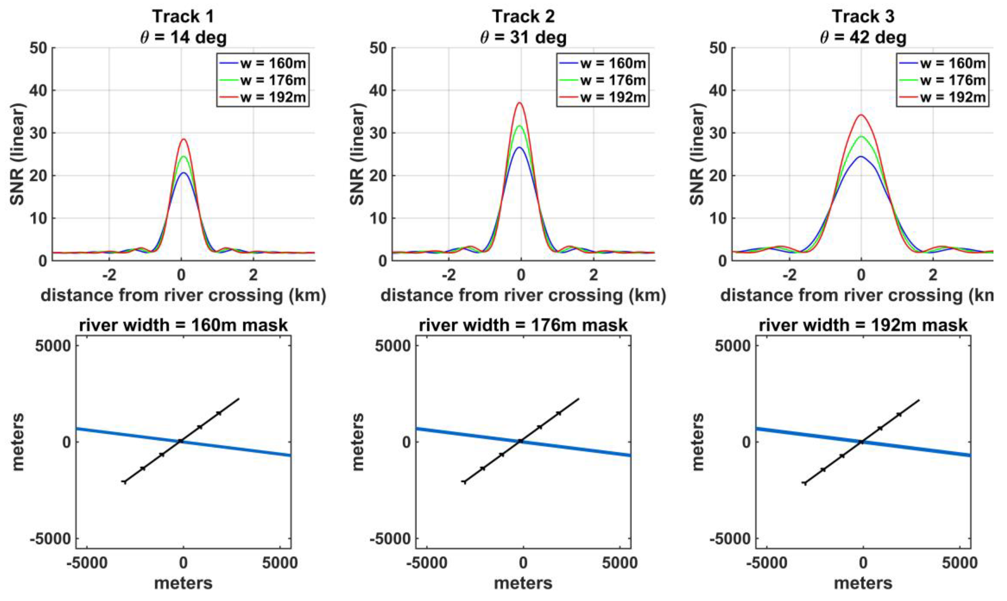
Figure 6.
SNR peak data points vs. river width (dots) and best fit regression (solid lines) for Track 1 (blue), Track 2 (green), and Track 3 (red) for oblique SP track crossings of a straight, isolated river.
Figure 6.
SNR peak data points vs. river width (dots) and best fit regression (solid lines) for Track 1 (blue), Track 2 (green), and Track 3 (red) for oblique SP track crossings of a straight, isolated river.
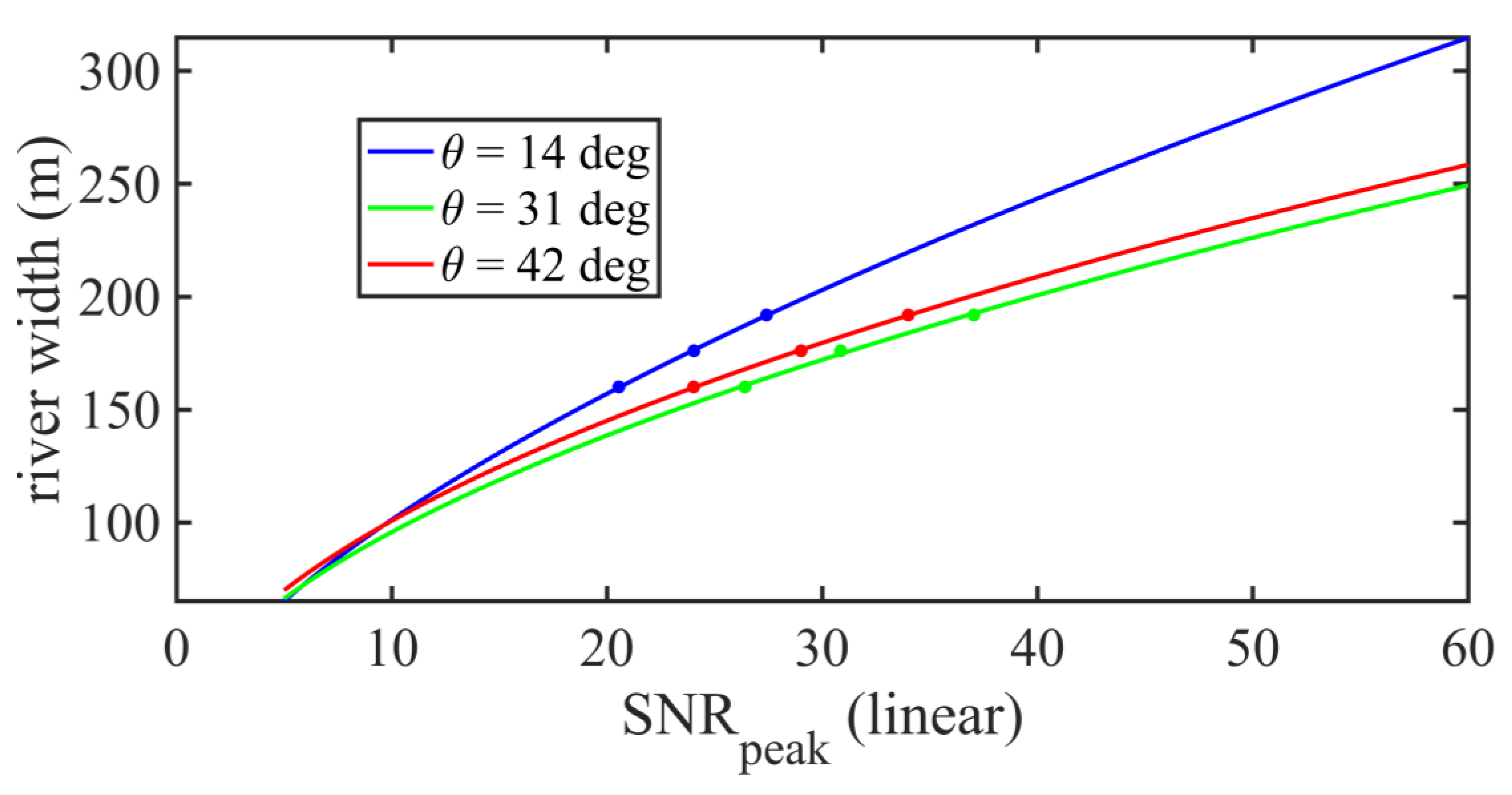
Figure 7.
Absolute value of the SNR perturbation as a function of the distance of a 1000m diameter circular lake from the center of the river for a perpendicular SP track river crossing. The dashed line indicates the standard deviation of noise in the SNR measurements.
Figure 7.
Absolute value of the SNR perturbation as a function of the distance of a 1000m diameter circular lake from the center of the river for a perpendicular SP track river crossing. The dashed line indicates the standard deviation of noise in the SNR measurements.
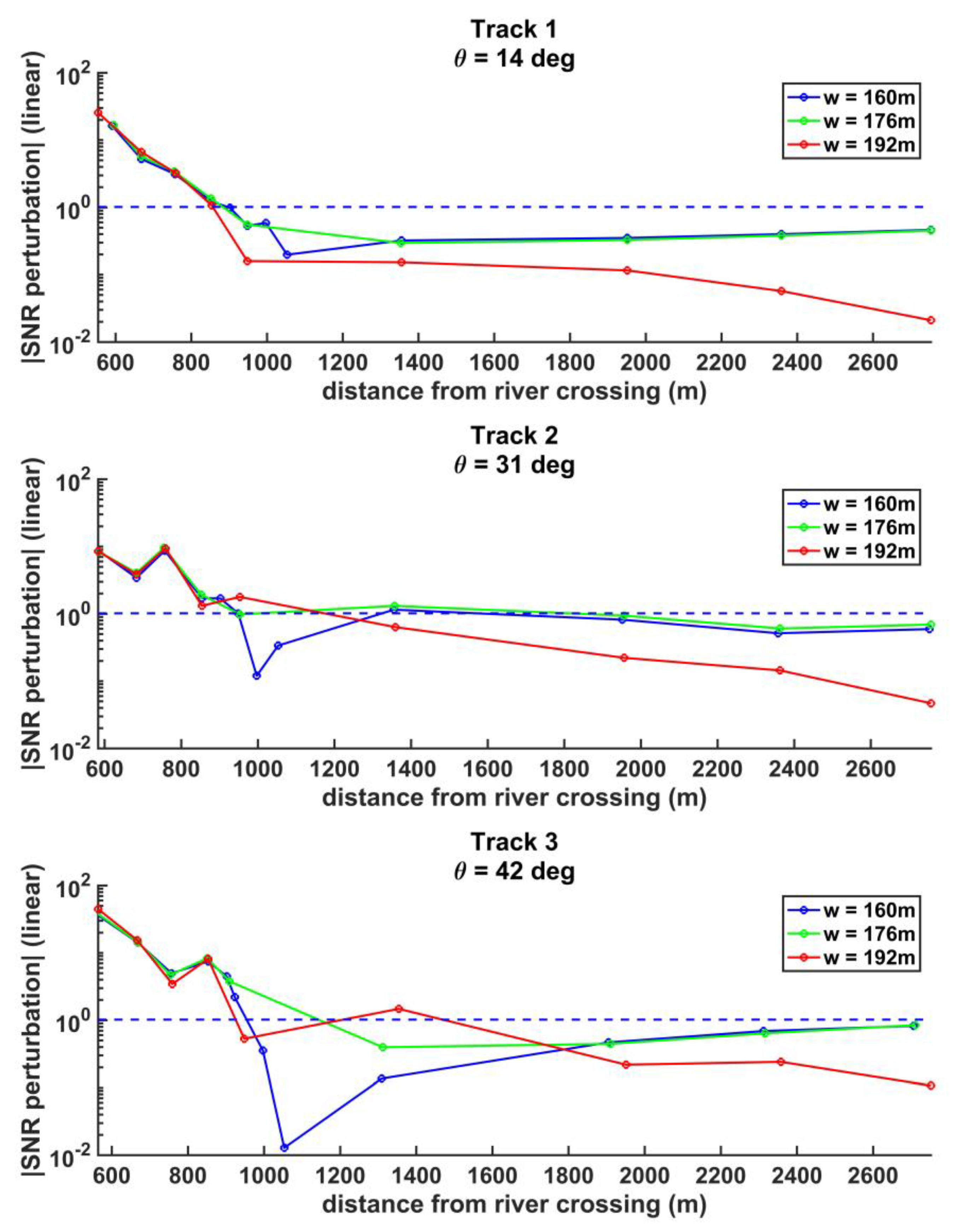
Figure 8.
Same as Figure 7 for an oblique 45 deg SP track river crossing.
Figure 8.
Same as Figure 7 for an oblique 45 deg SP track river crossing.
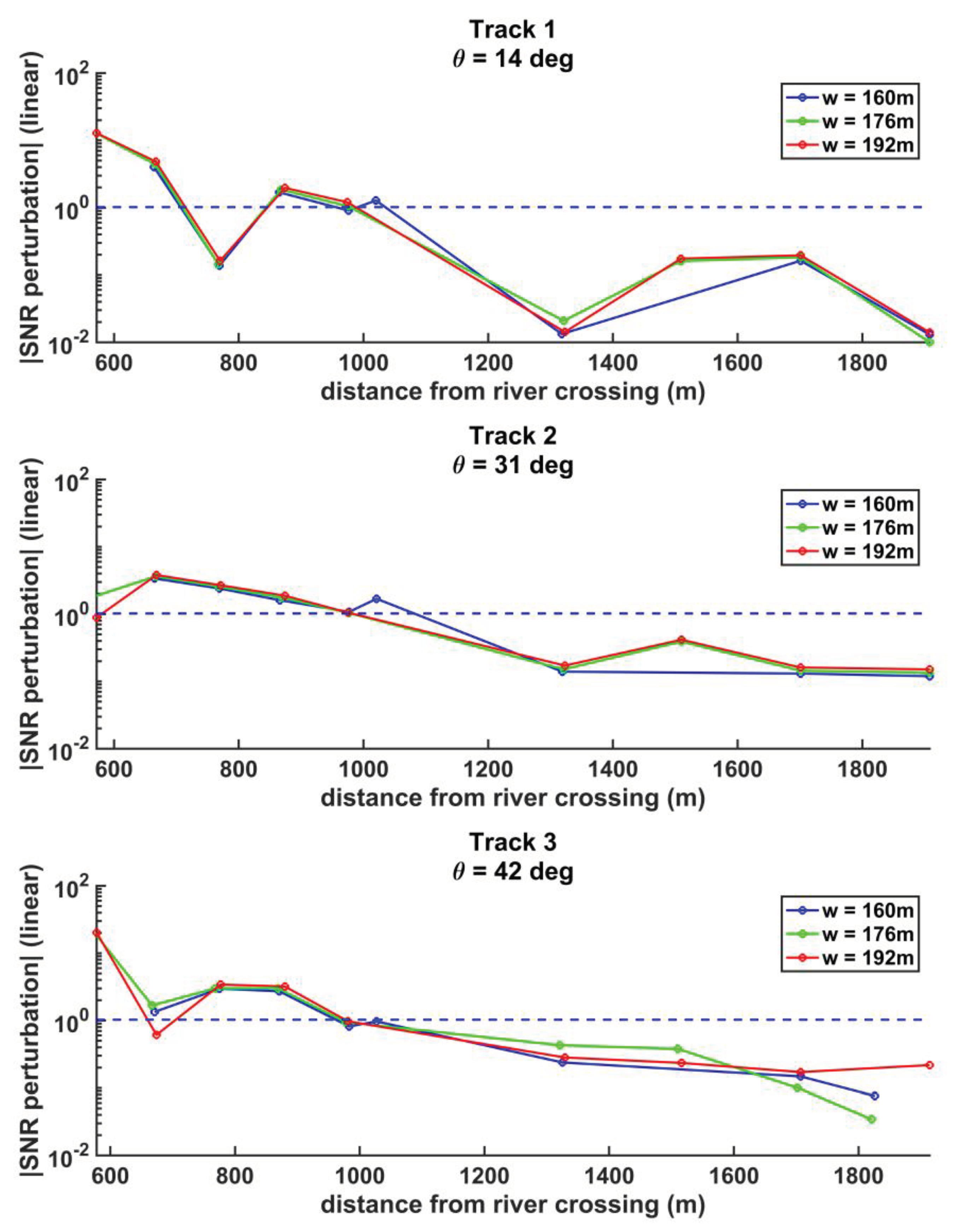

Table 1.
Calculation of the calibration offsets for the three E2ES validation cases shown in Figure 1.
Table 1.
Calculation of the calibration offsets for the three E2ES validation cases shown in Figure 1.
| Río Santiago | Lake Ilopango | Roosevelt River | |
|---|---|---|---|
| Observed incoherent mean SNR (dB) | 2.56 | 2.36 | 2.78 |
| Observed coherent peak SNR (dB) | 20.38 | 10.33 | 21.56 |
| E2ES incoherent avg (dB) | -181.86 | -189.70 | -182.54 |
| E2ES coherent peak (dB) | -163.23 | -162.95 | -158.24 |
| Incoh. calibration term (E2ES/obs) (dB) | -184.42 | -192.06 | -185.32 |
| Coh. calibration term (E2ES/obs) (dB) | -183.61 | -173.28 | -179.80 |
Table 2.
Parameters for the three input geometry tracks used for the simulated river cases.
| Track 1(Lake Ilopango) | Track 2(UHE Rondon II) | Track 1 (Marañón River) | |
|---|---|---|---|
| Observed incoherent mean SNR (dB) | 1.98 | 2.30 | 2.64 |
| Observed coherent peak SNR (dB) | 19.83 | 21.90 | 22.78 |
| E2ES coherent peak (dB) | -150.97 | -151.64 | -159.93 |
| E2ES incoherent avg (dB) | -183.79 | -180.34 | -180.92 |
| Incoh. calibration term(E2ES/obs) (dB) | -185.77 | -182.64 | -183.56 |
| Coh. calibration term (E2ES/obs) (dB) | -170.80 | -173.54 | -182.71 |
| Maximum | 1.00 | 1.00 | 1.00 |
| (GPS EIRP) (Watts) | 1709 | 1250 | 1060 |
| (dB) | 8.5 | 12.9 | 13.2 |
| (deg) | 14 | 31 | 42 |
| (km) | 20209 | 20627 | 21610 |
| (km) | 541 | 587 | 690 |
Table 3.
Model regression constants for the straight river with perpendicular SP track cases.
| Incidence angle | a | m | b |
|---|---|---|---|
| 14 deg (Track 1) | 23.77 | 0.6332 | -0.5105 |
| 31 deg (Track 2) | 20.91 | 0.6133 | -0.6978 |
| 42 deg (Track 3) | 19.17 | 0.5916 | -0.5851 |
Table 4.
Model regression constants for a straight, isolated river with SP tracks at an oblique approach angle.
Table 4.
Model regression constants for a straight, isolated river with SP tracks at an oblique approach angle.
| Incidence angle | a | m | b |
|---|---|---|---|
| 14 deg (Track 1) | 23.74 | 0.632 | -0.356 |
| 31 deg (Track 2) | 27.51 | 0.537 | -0.98 |
| 42 deg (Track 3) | 30.22 | 0.525 | -0.315 |
Table 5.
River width precision ( in meters for the straight river with perpendicular SP track cases.
Table 5.
River width precision ( in meters for the straight river with perpendicular SP track cases.
| Incidence angle | |||
|---|---|---|---|
| 14 deg (Track 1) | 5.1 | 4.8 | 4.6 |
| 31 deg (Track 2) | 3.6 | 3.4 | 3.2 |
| 42 deg (Track 3) | 2.7 | 2.5 | 2.4 |
Table 6.
River width precision ( in meters for a straight, isolated river with SP tracks at an oblique approach angle.
Table 6.
River width precision ( in meters for a straight, isolated river with SP tracks at an oblique approach angle.
| Incidence angle | |||
|---|---|---|---|
| 14 deg (Track 1) | 4.4 | 4.1 | 3.9 |
| 31 deg (Track 2) | 3.4 | 3.1 | 2.9 |
| 42 deg (Track 3) | 3.6 | 3.4 | 3.1 |
Table 7.
River width retrieval accuracy ( in meters for the perpendicular and oblique approach angles.
Table 7.
River width retrieval accuracy ( in meters for the perpendicular and oblique approach angles.
| Approach angle | Track 1 | Track 2 | Track 3 |
|---|---|---|---|
| Perpendicular | 0.48 | 0.68 | 0.57 |
| Oblique | 0.04 | 0.04 | 0.03 |
Table 8.
Total river width retrieval error (uncertainty), , in meters for the perpendicular and oblique approach angles.
Table 8.
Total river width retrieval error (uncertainty), , in meters for the perpendicular and oblique approach angles.
| Approach angle | Track 1 | Track 2 | Track 3 |
|---|---|---|---|
| Perpendicular | 5.12 | 3.66 | 2.76 |
| Oblique | 4.40 | 3.40 | 3.60 |
Disclaimer/Publisher’s Note: The statements, opinions and data contained in all publications are solely those of the individual author(s) and contributor(s) and not of MDPI and/or the editor(s). MDPI and/or the editor(s) disclaim responsibility for any injury to people or property resulting from any ideas, methods, instructions or products referred to in the content. |
© 2024 by the authors. Licensee MDPI, Basel, Switzerland. This article is an open access article distributed under the terms and conditions of the Creative Commons Attribution (CC BY) license (http://creativecommons.org/licenses/by/4.0/).
Copyright: This open access article is published under a Creative Commons CC BY 4.0 license, which permit the free download, distribution, and reuse, provided that the author and preprint are cited in any reuse.


