

Submitted:
19 March 2024
Posted:
20 March 2024
You are already at the latest version
Abstract
The classical Lotka-Volterra predator-prey model is globally stable and uniformly persistent. However, in real-life biosystems extinction of species due to stochastic effects is possible. In this paper, we consider the classical Lotka-Volterra predator-prey model under stochastic perturbations. For this model, using an analytical technique based on the direct Lyapunov method and a development of the ideas of R.Z. Khasminskii, we find the precise sufficient conditions for the stochastic extinction of one and both species and the precise necessary conditions for the stochastic system persistence. The stochastic extinction occurs via a process known as the stabilization by noise of the Khasminskii type, and, in order to establish the sufficient conditions for extinction, we found the conditions for the stabilization.
The analytical results are illustrated by numerical simulations.
{\bf Keywords:} stochastic perturbations, white noise, Ito's stochastic differential equation, the Lyapunov functions method,
stability in probability, stabilization by noise, stochastic extinction, persistence.
Keywords:
Ito's stochastic differential equation
; the Lyapunov functions method
; stability in probability
; stabilization by noise
; stochastic extinction
; persistence
1. Introduction
Let us consider the classical predator-prey model [1,2,3,4,5]
where all parameters are positive. This model was suggested independently by Volterra and Lotka, and its properties are well studied. Specifically, the model has three equilibria, namely (i) the zero equilibrium , (ii) the predator-free equilibrium on the x-axis, and (iii) the positive equilibrium , where both species coexist. Coordinates and are defined by the equalities
with the solution
Here, the parameter has a transparent biological meaning: it is the predator’s basic reproduction number, i.e., a number of the offspring that reach the reproductive age produced per capita of the predator under the most favourable conditions when and . The concept of the basic reproduction number is originated in the infectious diseases dynamics, where it is proved to be exceptionally successful. We believe that this concept is very convenient in modelling population dynamics as well.
The principal global asymptotic properties of model (1.1) are summarized by the following theorem [1,3]:
Theorem 1.
For the system (1.1) the following statements are true:
(1) If , then the coexisting equilibrium exists and is globally asymptotically stable, while the predator-free equilibrium is unstable (a saddle points).
(2) If , then system (1.1) has no coexisting equilibrium state, and the equilibrium is globally asymptotically stable.
(3) The zero equilibrium is always unstable (a saddle point).
A principal property of the Lotka-Vo;terra model is its persistence. At the same time, it was observed that in real-life biosystems species can extinct due to stochastic fluctuations. Objectives of this paper is to analytically study how stochastic effects affect the model dynamics, and, in particular, its persistence and species extinction. We consider, therefore, the Lotka-Volterra model under stochastic perturbations of the white noise type that are postulated proportional to the system current state. Such type of perturbations appear to be the most natural for models motivated by biological applications.
To explore the persistence or stochastic extinction in the stochastic model, in this paper we employ a recently developed by the authors method [6,7] that is based on the direct Lyapunov method [8] and, in particular, on the development of ideas of R.Z. Khasminskii [9]. Specifically, in line with Khasminskii’s idea, we suggest that the sufficient conditions for the stochastic extinction are the conditions for the reversion of the stability of the trivial equilibrium state (so called “stabilisation by noise”). Application of this idea to the model ensures the precise sufficient conditions for species extinction (and, hence, the precise necessary conditions for persistence).
To apply the Khasmiskii’s idea to the models originated in mathematical biology, we extended it to multi-dimensional nonlinear systems and exploited the concept of the stability of invariant sets. That is, instead of the stability of the trivial equilibrium state of a linear 1-dim stochastic equation, as in [9], we study of the stability of the coordinate axes of a nonlinear stochastic system.
2. Predator-Prey Model under Stochastic Perturbations
Let be a complete probability space, be a nondecreasing family of sub--algebras of , i.e., for , be the mathematical expectation with respect to the measure .
Let us assume that the model (1.1) is influenced by stochastic perturbations that are of the white noise type and are of magnitudes proportional to the current population size. Then the system of ordinary differential equations (1.1) transforms to the following system of Ito’s stochastic differential equations (SDE) [10]:
Here and are constants, and and are the mutually independent -adapted standard Wiener processes.
Before we proceed to the model analysis, let us recall the basic definition of persistence and extinction that are applicable to systems (1.1) and (2.1) [11,12,13]:
Definition 1.
Species x is weakly persistent if for all , .
Species x is persistent if for all , .
Species x is uniformly persistent if for all , .
Species x extincts if for all , .
The same definitions are applicable for species y.
By term "stochastic extinction" we imply the extinction due to stochastic processes only. That is, stochastic extinction occurs under the conditions when the corresponding deterministic system is persistent.
Lemma 1.
The positive quadrant is an invariant set of stochastic system (2.1).
For proof it is enough to note that the solution of system (2.1) is presented in form [10]
Lemma 2.
If , then set
is in mean a positive invariant and attractive set of system (2.1).
Proof.
Let L be the generator [10] of system (2.1). The Lyapunov function satisfies
That is, ensures that for all , . By Dynkin’s formula [10]
inequality for implies that . That is, for all and Lyapunov function decreases as t grows. Therefore, the mathematical expectation of the solutions with positive initial conditions converge to the region M and remain there. □
We would like to remind that is the environment currying capacity for the prey. Lemma 2 implies that, due to stochastic fluctuations, in system (2.1) the mathematical expectation for the prey population exceeds the deterministic currying capacity K and varies within the range . This fact indicates a necessity to introduce, alongside to the deterministic currying capacity K, the stochastic currying capacity
Using this notation, set . Furthermore, the concept of stochastic crying capacity naturally leads to a concept of the stochastic predator’s basic reprobation number
Lemma 3.
If , then the zero equilibrium is stable in probability.
Proof.
Using the Lyapunov function , for all we have
Therefore, semi-axis (as a solution of the first equation of system (2.1)) is stable in probability [9].
Next, consider Lyapunov function , if , and , if . If , then
From the above-said arguments, it follows that , and, hence, the condition ensures that inequality holds for all .
If , then Lyapunov function satisfies
As by the arguments above, we obtain that for all , . Therefore, in the both cases, namely for and , solution of the second equation of system (2.1) is stable in probability. That is, the zero equilibrium of system (2.1) is stable in probability [9]. This completes the proof. □
It was shown in [6], that the condition is the necessary condition for prey’s persistence. It is hardly surprising, that the extinction of prey immediately leads to the extinction of predators.
Authors also would like to mention that Lyapunov functions of the type that was used in the proof were invented by R.Z. Khasminskii [9]. The inversion of the stability for larger perturbations, such as Lemma 3 describes, is usually referred to as the stabilization by noise.
Lemma 4.
If and , then for the system of stochastic differential equations (2.1) the set (an interval on the positive semi-axis ) is stable in probability.
Proof.
From (2.3), for Lyapunov function , we have that holds for all , . Therefore, the solution of the second equation of system (2.1) is stable in probability. Besides, ensures that . Besides, by Lemma 2, for all positive initial conditions, there is a finite such that holds for all .
That is, the lemma hypotheses ensue that holds for all positive initial condition and for . This completes the proof. □
Summarizing statements of Lemmas 3 and 4, we come to the following theorem.
Theorem 2.
(1) Conditions and are sufficient conditions for the prey stochastic extinction (the extinction by probability).
(2) If , then both species, namely, the prey and the predator, extinct (by probability).
(3) is necessary for the stochastic system persistence.
(4) and either , or are necessary for predator’s persistence.
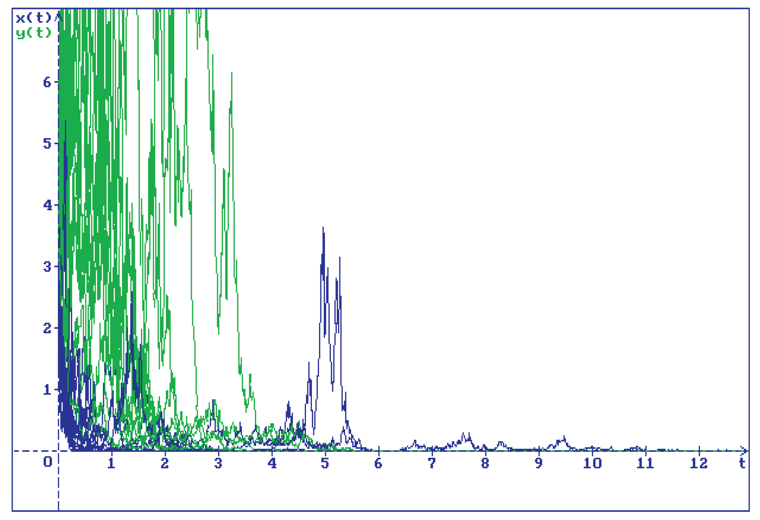
Figure 1 and Figure 2 illustrate the predator extinction due to stochastic perturbations for the case and , respectively. Figure 3 illustrates the stochastic extinction of both species for case and .
Note that for the numerical simulation of the Wiener process trajectories, a special algorithm described in detail in [8] has been used.
The authors would like to attract readers’ attention to the fact that in Figure 1 and Figure 2, as , the prey population oscillates around a certain interval . (In Figure 1 and Figure 2, .) In fact, in the absence of the predator (that is, for ), the first equation of the system of stochastic differential equations (2.1) is equivalent to the stochastically perturbed logistic equation of a single population growth that was studied by the authors in [6]. In [6], for this equation the authors established the existence of a stable in mean interval on the x-axis and show that the trajectories oscillate around this interval. (In notation of this paper, the interval is .) Recalling that the x-axis is an invariant set of system (2.1) and that solutions are continuous, it is easy to see, that, as , the solution of system (2.1) tends to that on the x-axis, and, hence, the interval in Figure 1 and Figure 2 corresponds to the stable interval found in [6].
3. Conclusions
In this paper, employing a recently developed by the authors technique based upon ideas of R.Z. Khasminskii, we found precise sufficient conditions for the stochastic species extinction and, hence, the precise necessary conditions for the species persistence for the classical Lotka-Volterra predator-prey model under stochastic perturbations proportional to the system current state. Please note that the found conditions of the extinction are sufficient, in probability. For this model, the stochastic extinction necessary occurs as a result of a phenomenon know as the stabilization by noise, and the conditions found in this paper are, in fact, the conditions for the reversion of the stability of the corresponding coordinate subspaces. This ensures that the conditions in this paper are the precise sufficient conditions for extinction, and, hence, the precise necessary conditions for the species persistence.
We would like to stress that the technique used in this paper can be applied for more complicated models (including nonlinear models), as well as for higher dimension models.
References
- Volterra, V. Lesons sur la Theorie Mathematique de la Lutte Pour la Vie; Gauthier-Villars, Paris, 1931.
- Freedman, H.I. Deterministic Mathematical Models in Population Ecology; Marcel Dekker, New York, 1980.
- Murray, J.D. Mathematical Biology; Springer, Berlin, 1989. [CrossRef]
- Brauer, F.; Castillo-Chavez, C. Mathematical Models in Population Biology and Epidemiology; Springer-Verlag, Heidelberg, 2000.
- Goh, B.S. Global stability in two species interactions. Journal of Mathematical Biology, 3 (1976) 313–318. [CrossRef]
- Korobeinikov, A.; Shaikhet, L. Global asymptotic properties of a stochastic model of population growth. Applied Mathematics Letters. 121 (2021) 107429. [CrossRef]
- Shaikhet, L.; Korobeinikov, A. Asymptotic properties of a Lotka-Volterra competition and mutualism model under stochastic perturbations. Mathematical Medicine and Biology, 2024 (in press). Published online: 24 February 2024. [CrossRef]
- Shaikhet, L. Lyapunov Functionals and Stability of Stochastic Functional Differential Equations; Springer Science & Business Media, Berlin, 2013.
- Khasminskii, R.Z. Stochastic stability of differential equations; Springer, Berlin, 2012 (in Russian, Nauka, Moscow, 1969).
- Gikhman, I.I.; Skorokhod, A.V. Stochastic differential equations; Springer, Berlin, 1972.
- Butler, H.; Freedman, I.; Waltman, P. Uniformly persistent systems, Proc. Am. Math. Soci., 96 (1986) 425–430.
- Freedman, H.I.; Moson, P. Persistence definitions and their connections, Proc. Am. Math. Soci., 109 (1990) 1025–1033 .
- Smith, H.L.; Thieme, H.R. Dynamical Systems and Population Persistence; AMS, Providence, 2011.
Figure 1.
15 trajectories of the solution of system (2.1) with , , , , , , and the initial conditions at point . It is easy to see that the predator species extinct, and all trajectories converges to interval on the x-axis (to oscillate around interval with the equilibrium in the centre of it)
Figure 1.
15 trajectories of the solution of system (2.1) with , , , , , , and the initial conditions at point . It is easy to see that the predator species extinct, and all trajectories converges to interval on the x-axis (to oscillate around interval with the equilibrium in the centre of it)
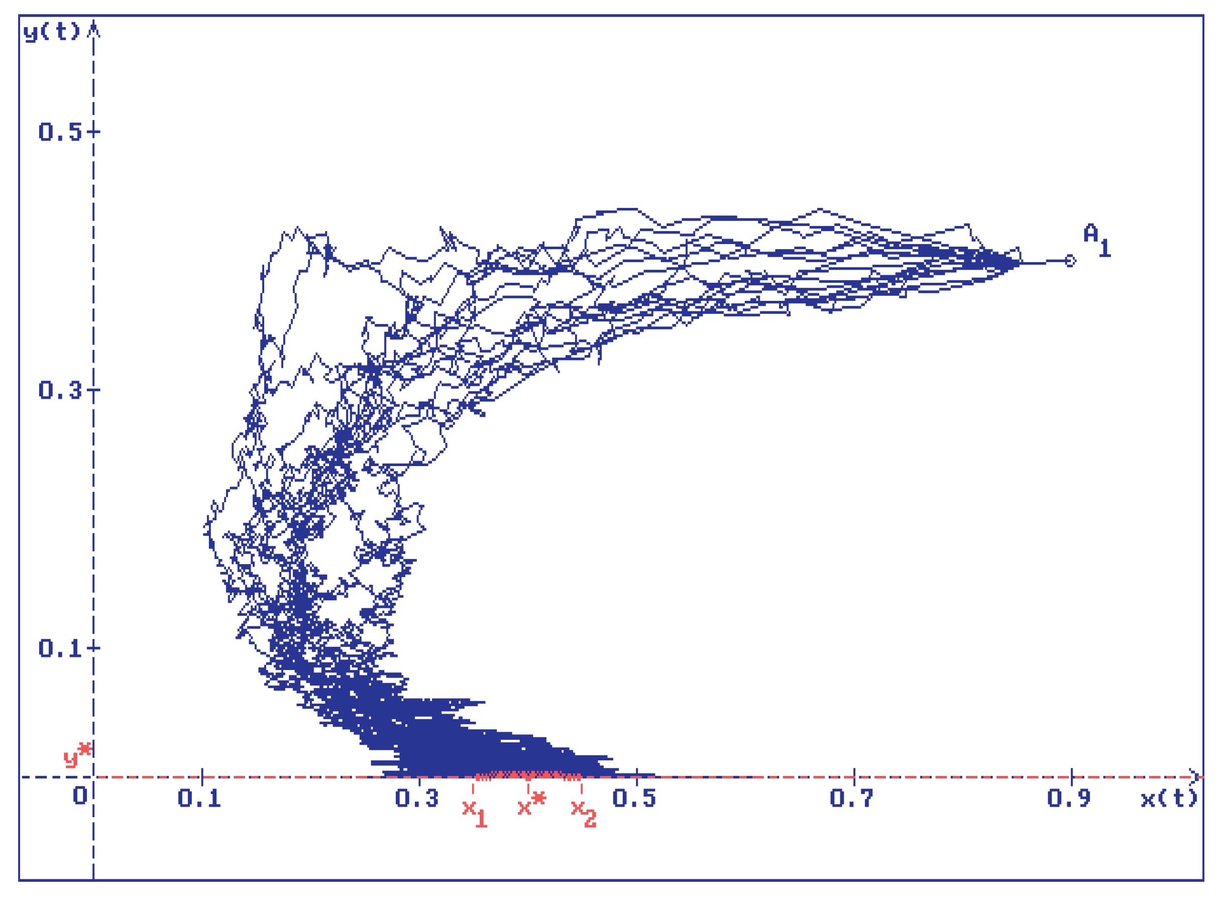
Figure 2.
15 trajectories of the solution of system (2.1) for the same values of the parameters as in Figure 1 and for initial conditions . It is easy to see that all trajectories (green lines) converge to , whereas (blue lines) oscillate around the interval
Figure 2.
15 trajectories of the solution of system (2.1) for the same values of the parameters as in Figure 1 and for initial conditions . It is easy to see that all trajectories (green lines) converge to , whereas (blue lines) oscillate around the interval
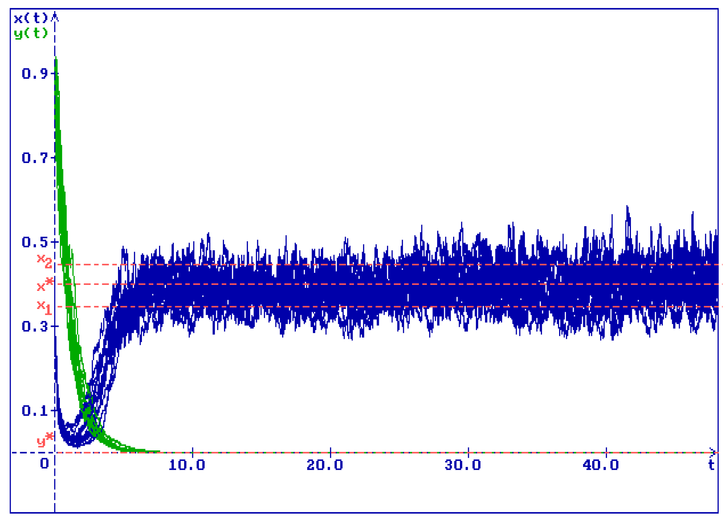
Figure 3.
15 trajectories of the solution of system (2.1) for , , , , , , and for initial conditions . All trajectories of (blue lines) and (green lines) converge to zero
Figure 3.
15 trajectories of the solution of system (2.1) for , , , , , , and for initial conditions . All trajectories of (blue lines) and (green lines) converge to zero
Disclaimer/Publisher’s Note: The statements, opinions and data contained in all publications are solely those of the individual author(s) and contributor(s) and not of MDPI and/or the editor(s). MDPI and/or the editor(s) disclaim responsibility for any injury to people or property resulting from any ideas, methods, instructions or products referred to in the content. |
© 2024 by the authors. Licensee MDPI, Basel, Switzerland. This article is an open access article distributed under the terms and conditions of the Creative Commons Attribution (CC BY) license (http://creativecommons.org/licenses/by/4.0/).
Copyright: This open access article is published under a Creative Commons CC BY 4.0 license, which permit the free download, distribution, and reuse, provided that the author and preprint are cited in any reuse.


