
Submitted:
18 March 2024
Posted:
19 March 2024
You are already at the latest version
Abstract
Pairs of potential and flow variables have long been established for interfacing object-oriented component models of physical systems. Recently, however, the use of triplets has been discovered for the purpose of robust modeling. New and powerful Modelica libraries have been developed such as the DLR ThermoFluid Stream library or the introduction of the Dialectic Mechanics library. Their use of triplets is entangled with a special modeling approach that uses Linear Implicit Equilibrium Dynamics. In this paper, we study the basic motivation of this approach, its benefits and drawbacks before we finally demonstrate how it beneficially impacts the generation of corresponding simulation code.
Keywords:
Object-oriented modeling
; Code Generation
; Modeling principles
1. Introduction
Pairs of potential (effort) and flow variables have long been established for the equation-based, object-oriented modeling of physical systems. For instance, Table 1 lists the interface currently in use for the Modelica Standard Library [1] and Table 2 lists the interface typically used for Bond-graphs [2,3].
For bond-graphs, the product of these pairs always represents a flow of energy. Although Modelica is less dogmatic, the flow of energy is still contained in the information of the connection pair.
The sheer size of the Modelica Standard Library, its industry wide adoption and also the use similar interfaces in a wide array of commercial tools provide empiric evidence that these pairs form very useful interfaces. And indeed, these pairs provide an answer for what is necessary for the object-oriented modeling of classic physical systems:
The equations whose solution represent a physical system can be distributed among its components
Thanks to these pairs, we can indeed distribute the equations of physical systems among different components. Unfortunately, the very same pairs are also the root cause for many very persistent problems encountered in the object-oriented modeling of physical systems.
- Irregular systems can be composed and are hard to diagnose.
- Very difficult handling of variable structure systems [4] (change of equations at run-time) due to the high index of the Differential Algebraic Equation (DAE) system.
- Very difficult code generation for large-scale system simulation [5] since often the complete equation system is needed for structural analysis
- Highly complex generation of simulation code requiring compilers that have high development costs. (The decade spanning effort of OpenModelica [6] provides evidence)
All these problems will be diminished (as demonstrated in later chapters), when we fulfill what is sufficient for object-oriented modeling:
Any valid combination of components (under rules of limited complexity) shall have a solution representing a physical system.
This statement centers on the ability to make an a-priori statement on the solvability of the modeled system and sadly (as we will see later), we can cannot fulfill this statement with the presented pairs of effort and flow. Instead, this paper suggests to use triplets as in Table 3.
Before we can aim to find a sufficient form and understand these triplets, we first need to understand what actually led us to the necessary pairs of potential (effort) and flow variables. Hence, we need to revisit the very basic fundamentals of classic physics.
2. The Principle of Stationary Action
The central question is what minimum interface is needed so that we can distribute the equation of systems in classical physics. The natural starting point is hence the most fundamental law forming the basis of all classical physics: the principle of stationary action also known as Hamilton‘s Principle. It is based on the action for an element moving along a path :
The action is the integral of the Lagrangian over the timespan . The Lagrangian itself can be expressed as the
difference between kinetic energy and potential energy . The principle of stationary action states that:
This principle is the basis of classic physics because it is also fulfilled by the underlying quantum physics although in a statistical manner as described by Feynman [7]. Yet for a sufficient large number of quantum events, the expected value will be fulfilled with great precision and an assumption of continuity can be made for macroscopic systems.
The principle of stationary action is here written for a conservative system. It would require extensions for non-conservative systems but there is no need here to complicate matters. In any case, the following literature may be advised [8,9,10,11] (chapter 20). A few points are however often underrepresented and hence deserve discussion here.
The principle of stationary action is based on the Lagrangian . We see that a different sign is applied for the kinetic energy than for all other forms of (potential) energy . The kinetic energy has thus a special role. Not only is its role special but also its form. The gradient of the kinetic energy forms a continuous bijective function for the total domain (whether relativistic or not), meaning that it has a well-defined inverse over the complete domain. This property is important for the discussion of another question: is there always a solution for the principle of stationary action?
Given that we can assume no strict restrictions on the complexity of the potential (other than having a derivative), it may seem unsolvable in the general case. Fortunately, the plot of Figure 1 indicates how to approach this problem.
This graph is a topological map of the action over time for paths of different constant velocity. We recognize that in this (completely arbitrary) example, the action has become a very complex function after a time-step of one second. However, for a small step of time, the action remains simple and well-natured. The explanation is straight forward: no matter how complex is shaped, it takes a motion through time and space to gather this complexity. Hence at , the well-natured kinetic energy dominates the action.
This means we can reliably solve the principle of stationary action if the step in time is small enough. What is small enough? Under the assumption of continuity, there is only one answer: . This leads us ultimately to the famous Euler-Lagrange equation and is also the explanation why time derivatives are so useful in physics.
Now we see also why it is so important that the partial derivative of the kinetic energy has a special form and a well-defined inverse. This ensures that the second term can always compensate the first in an unambiguous way. Please note that such a general statement on solvability is extremely helpful.
For illustration, let us now apply the Euler-Lagrange to the following example system for the pressure wave of a fluid in a pipe. The derivative of our path: represents the volume flow . Correspondingly the path then represents the shift in volume .
- The kinetic energy is then defined as: with being the density and the inertance defined by the geometry length and cross section :
- The potential energy can be formulated by where is the bulk modulus and a reference volume.
The Lagrangian is now defined by:
and we can apply the Euler-Lagrange equation which results in:
Fortunately, many terms vanish when taking the partial derivative and the resulting equation is a differential equation of second order that expresses the wave in the fluid based on its volumetric shift:
The elegance of the Euler-Lagrange equation is that it provides a solution of dimensions with equations for an underlying variational problem that is actually a dimensional problem (please note that one shall treat and as independent variables [11]).
This elegant “compression” is however working against the intent of object-oriented modeling: for examples of higher dimensions, it will be very difficult to redistribute the equations to individual components. Hence the result of Euler-Lagrange is mostly unsuited for object-oriented modeling.
Fortunately, there is an alternative form that can be achieved by the Legendre transformation that transforms the Lagrangian into the Hamiltonian . The stationary action principle can now be reformulated for our example. For the Legendre transformation we require the generalized momentums that are defined as
For illustration, let us reiterate our previous example. Based on the former Lagrangian, we can determine the generalized momentum :
Using to express the kinetic energy is then applied for composing the Hamiltonian :
Given the Hamiltonian, we can now apply the famous pair of Hamilton equations:
In our example, these translate to:
We now get first order differential equations, based on generalized position and generalized momentum. These equations express the same system as the previous solution derived by Euler-Lagrange. (simply differentiate the first equation and eradicate by substitution). Different from the Euler-Lagrange solution, these equations can be nicely distributed among components, especially if we reformulate them based on a corresponding pair. In our setting it is natural to choose the volume flow and the pressure as pair. The corresponding components are presented in Table 4, row 1 and 2.
We can then choose to model a different storage of potential energy such as gravitational pressure. Even though all our derivations were done on conservative systems, the same pair can be used to model non-conservative components such as the friction of a valve. These two additional components are presented in Table 4, row 3 and 4.
Given these 4 components of Table 4 and the pair of effort and flow, we can now assemble a more complex system and for instance model the example of 3 communicating vessels as in Figure 2. Classic object-oriented modeling becomes functional.
In the corresponding simulation results (Figure 3) we can see the oscillation that result from the natural parameters of water. As typical for many systems the exchange between potential and kinetic energy is of high frequency.
3. From Necessary to Sufficient
We have seen that the well-known pairs of potential and flow variables can be derived from the Hamiltonian form of the principle of stationary action (although not always in the exact same way as for the hydraulic example above).
Different form the Lagrangian , the kinetic energy loses its special role in the Hamiltonian . Treating all energy forms equal may deceivingly suggest that energy flows are all what the modelers needs (Bond graph modelling is a prime example of this fallacy). Yet, whereas each valid Hamiltonian represents a sum of energy terms, not all sums of energy terms represent a valid Hamiltonian. This leads to a serious problem for object-oriented modeling. Whereas the pairs are necessary to redistribute the equations resulting out of a valid Hamiltonian, only very few recombination possible by these pairs form a valid Hamiltonian. This implies that the modeler can formulate non-physical systems too and modelers even do this on purpose (albeit often without being fully aware of the consequences). For instance, let us consider the following recombination of components as depicted in Figure 4.
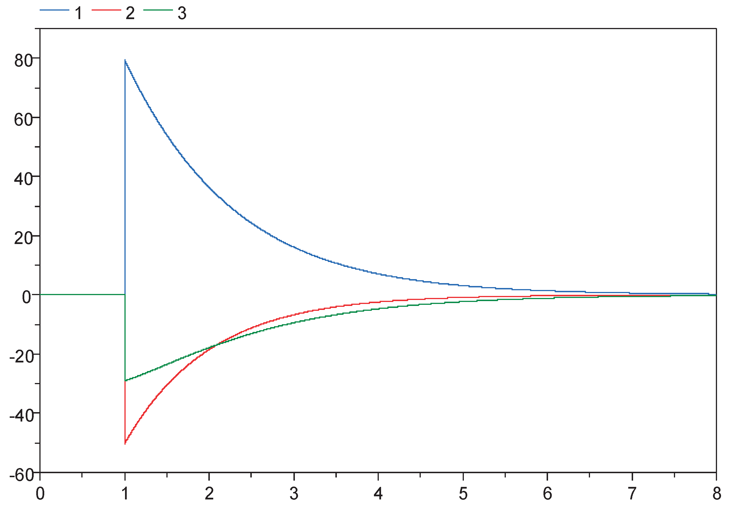
Here the modeler has now completely removed the inertia and compressibility of water from the model. This means that there is no representation of the kinetic energy anymore. We have removed exactly the component that is required to formulate the principle of stationary action and guarantee its solvability. Instead we now use the pairs to formulate a constraint problem in the domain of energy. Whether this can be solved is in general undefined. And indeed, we have to solve a non-linear equations system in this example to perform the simulation. In this example, the solution could reliably be found during simulation time but in the general case no statement on solvability can be given.
It is however important to recognize that modelers do such things (mostly) not out of malevolence or ignorance but to solve relevant problems. The slight additional cost of solving the non-linear equation system was rewarded in this example by the much higher gain of removing the high frequency from the system enabling a very efficient simulation of the system (albeit significantly altering the trajectory).
Figure 5.
Simulation result of the model of Figure 4, showing the 3 volume flows going through the tank’s orifices. In this simplified model the high frequency has been eliminated and the flow rate is now dominated by the resistance.
Figure 5.
Simulation result of the model of Figure 4, showing the 3 volume flows going through the tank’s orifices. In this simplified model the high frequency has been eliminated and the flow rate is now dominated by the resistance.
Hence, what would we need to do to ensure solvability and also enable powerful modeling approach? Essentially, we have to fulfill two criteria:
- (a)
- Ensure that the kinetic energy is always sufficiently represented so that we can guarantee solvability according to the steady-action principle.
- (b)
- Enable the modeler to reduce the interaction between kinetic and potential energies to key points in the system so that irrelevant high frequency behavior can be effectively suppressed.
For some domains, these two criteria can be met in a methodological sound manner by going from a pair to a triplet.
Part of this triplet is a pair that expresses the kinetic energy. This pair is accompanied by a signal that describes the non-linear configuration under which the kinetic energy can be exchanged. This rather abstract picture is best described by concrete examples. One for thermo-fluid systems and one for mechanical systems.
In the following we discuss the modeling of two domains using triplets.
3.1. Triplet Interface for Thermofluid Systems
Here is the triplet interface for thermo-fluid streams:
- : inertial pressure (potential)
- : mass-flow rate (flow)
- : Vector representing the thermodynamic state of the medium (signal)
- -
- : steady-mass flow pressure
- -
- : steady-mass flow enthalpy
- -
- : mass fractions
Key to understand this interface is the dynamic of the inertial pressure . It represents the pressure needed to accelerate a mass-flow which forms linear law based on the inertance [12,13] of the fluid :
The inertance is thereby independent of the thermodynamic state of the fluid and just defined by the geometry of the flow with the lengthand cross section area :
If we now enforce that the inertance law is part of every single component, we have fulfilled criterion (a).
To fulfill criterion (b), we decompose the pressure into two components:
The complement to is hence the newly defined steady-mass flow pressure For the steady-state with a constant mass flow rate, will go to zero and which explains its name.
A very elegant way to reduce the interaction points between potential energies and kinetic energy is to use to form an approximation for the thermodynamic state of the fluid. Furthermore, where it is not reasonable to mix pressure, it is feasible to provide mixing laws for . This enables an explicit downstream computation of The kinetic energy will then only interact at the boundaries of streams which are either volume elements or sources and sinks. At junctions, the kinetic energy of different streams may interact with each other. Ultimately this means that a different spatial resolution is applied for the effects of than for . This assumption is in line with many modeling tasks and deviations are limited to rapid transients where model uncertainty is typically very high. At steady mass flows there is no difference which is important for most applications.
The resulting computational scheme is that all the non-linear computations regarding the thermodynamic state including properties like viscosity, heat conductivity or density are performed in explicit form downstream. This means that the signal is always computed from the source to the sink. To ensure this, all circular flows need to contain at least one volume. A linear system then computes the time derivative of all mass-flows. This system is formed by the equation for the pairs of and . It is guaranteed to be linear because of the characteristics of and it will be regular since all inertances are strictly greater than zero.
The reader is advised to literature [14,15] to follow the above statements in detail. Revisiting our example of section 2, there is fortunately a less complex replacement model. Since our models assume constant density and viscosity, there is no need for the decomposition of and for the signal . The solution would (in this particular case) be equivalent to represent the inertance for each mass-flow but we are free to neglect the compressibility. The corresponding diagram is shown in Figure 6 and the simulation result in Figure 7. Also because each mass flow is represented by the sum of all of its inertances, the frequency of the response is low.
3.2. Triplet Interface for Mechanical Systems
It is possible to formulate a similar triplet to model multi-body mechanics:
- : velocity (potential)
- : force (flow)
- : position (signal)
Where and represent positions and velocities in a generalized way for both translatory and rotational motion.
The product of velocity and force thereby represents a flow of energy which will contain also the kinetic energy. To ensure criterion (a), we simply must enforce that there are no massless components or (by the means of connection rules) that there is at least a mass representing all degrees of freedom of a kinetic chain.
To fulfill criterion (b), we have to address the elements of a multi-body system that define the degrees of freedom for the system: the joint elements. These are typically revolute joints or prismatic joints but exist in various combinations that define a different set of positional states. Naturally, the velocity is defined as direct derivative of the position and the acceleration as second derivative:
In section 3.1, we have reduced the interaction of kinetic and potential energy by lowering the spatial resolution of the kinetic part. For multi-body mechanics we have to reduce the temporal resolution of the kinetic part. We can do so by applying a first-order filter:
Using the time constant , we can now effectively limit the occurring frequencies of the mechanical system (at the cost of becoming more energy dissipative) without modifying the steady-state solution.
Just for the sake of quick illustration: Figure 8 from [16] shows the dynamics of a lightweight object moved in clamp modeled by a very stiff spring. The figure simply illustrates how the oscillatory dynamics is approximated with a replacement dynamics leading to the same (quasi) steady-state solution.
Using the triplet, we can formulate a difference between the motion in the elastic regime and the velocity in the kinetic regime . Because of this separation of two regimes, the author has denoted it as dialectic mechanics. The interface enables again that all non-linear equations regarding the geometrical configuration can be formulated in explicit form from the root of the kinematic chain to its end by the signal . To ensure this tree structure, all kinematic loops must contain a flexible element. The pair of and then sets up a linear system of equations for the kinetic energy.
4. Triplets and Object-Oriented Modeling
The two triplets presented in section 3 can be directly transformed into code of the equation-based, object-oriented language Modelica. Table 5 contains the corresponding code. For both domains, corresponding Modelica libraries have been developed.
The DLR ThermoFluid Stream Library [15] is a fully functional open-source that is already in use both in industry and academia. Figure 9 shows an exemplary model diagram of the thermal architecture of an electric car. We can clearly see that a complex architecture is nicely composed out of its individual components. The end-user is not directly confronted with the triplets. The modeler simply needs to take care about the connection rules that all loops contain at least one volumetric element.
The library for Dialectic Mechanics is still under internal development and testing. Figure 10 shows the model diagram of a kinematic loop for a hypothetical landing gear kinematic. This demonstrates that also here, complex systems can be composed in an object-oriented fashion and the end-user simply has to uphold the connection rules. The kinematic loops a closed by flexible elements and each chain contains at least one mass.
Using Modelica for these examples, a complete DAE system is built based on the composed models. The complete system of equations is then flattened (meaning that all equations are collected in a global set) and then state variables are selected and symbolic index reduction (as for example in [18]) is performed to transform the DAE into a set of Ordinary Differental Equations (ODEs). This typically results in a larger piece of simulation code where all variables are globally collected.
5. Triplets and Linear Implicit Equilibrium Dynamics
We have derived the triplet interface out of the motivation to have a robust modeling interface that ensures solvability and yet enables effective modeling by the suppression of high frequency behavior (that occurs in real physical systems). It is remarkable that for both cases the resulting computational structure of the complete system is of a particular form that we define here as Linear Implicit Equilibrium Dynamics (LIED).
A DAE system with potential state derivatives , time and algebraic variables
is defined as LIED system when it can be transformed into the following form:
We see that both the algebraic variables as well as the state derivatives can be split into a fully explicit part () and a part () with a linear system in implicit form expressed by the matrix . Furthermore, the following conditions shall hold true:
These conditions essentially mean that it is allowed to perform certain symbolic mechanism of index reduction such as the dummy derivative method [18] originating from Pantelides [19]. Using this method, states variables of can be transformed to algebraic variables in and further derivatives may be added to or . In practice this is important because it means that the linear implicit dynamics can be expressed by far fewer states than suggested in the original DAE formulation.
To get a practical feeling for this LIED form, let us discuss the decomposition of the linear and non-linear part, for the presented triplets.
- For thermofluid streams, the signal for the thermodynamic state will be part of. States associated with this state such as the temperature of a volume will be part of . A subset of the flow variables will form . The subset is chosen in such a way that all streams are described by in a non-redundant way. The redundant mass flows as well as the inertial pressures become part of
- For dialectic mechanics, the signal for the position will be part of The potential and flow variables of the interface and will be part of . The state vector is typically empty. The members of are chosen from the internal variables in such a way that the motion of the kinematic chain is described in a non-redundant way. For each degree of freedom its kinetic velocity and its position form state variables in .
6. How to Create Simulation Code for LIED Systems?
The original intention of the LIED approach was simply to ensure that no non-linear system is created in implicit form that spans across the components and hence a robust solution of the model evaluation could be taken for granted, given robust component models. When we started with it, we expected it to be the only notable change from other DAE models in Modelica and that all other features of a of code generation (as briefly outlined at the end of section 4) would basically remain untouched.
However, over time, it was gradually recognized that LIED systems are much simpler to transfer to simulation code than general DAEs. Let us go through these observed simplifications one-by one:
- Because we avoid the creation of non-linear equation systems, we do not need a non-linear equation system solver anymore.
- For the same reason, constraint equations among potential states cannot be non-linear and hence no dynamic state selection is needed [20]
- Even stronger: we can select the states on component level. For example, the stars in Figure 9 and 10 mark those components that define states in .
- Because we can select the states on component level, this means that the dummy-derivative method can be applied also on component level before system composition.
- Since the goal of the linear equation system is to have a synchronized replacement dynamics towards the equilibrium, we know suitable tearing variables for this system. These will be the linear state derivatives: or at least a subset of it.
- The residual for a tearing variable can be attributed to the same component as the tearing variable.
The terminology of the last two points may require further explanation. A tearing variable is a variable that can be used to probe the reaction of an algebraic system which is assessed by a corresponding residual. If the system is linear: , the probing can be used to construct M and w and find the solution for w.
All of the points above represent observations resulting from modeling many components and system examples using the LIED approach. However, these observations have profound implications. For each component we know:
- the set of pairs of state-variables and their derivatives it adds to the system.
- the set of pairs of tearing and residual variables it adds to the system.
If this is the case, we can basically causalize everything already on the component level. In concrete terms, this means for each component:
- we stipulate the states
- we stipulate the tearing variables of the linear system and the corresponding residuals
- we perform the dummy derivative method on those equations where necessary.
- we define the causality of the interface variables
- we causalize all equations into assignments in a particular order
- we group the list of assignments depending on their dependence of the inputs.
Practical experience so far indicates that performing index reduction to transform to the LIED form can be performed in a very methodical and deterministic manner. It is thus far easier to generate simulation code for the LIED modeling approach than it would be for general higher-index DAEs. Neither there is a need for global flattening anymore nor are elaborate heuristics needed for the selection of state or tearing variables. Indeed, the generation of simulation code is so easy that a direct implementation in C++ becomes feasible. To demonstrate this, the following code excerpts illustrate the implementation for a thermofluid stream library (using idealized water) in C++.
First, we have to define the interface. This is naturally more tedious than in a language like Modelica because there is no direct support in the C++ language. Yet, it is feasible and after all, interfaces only need to be defined once:
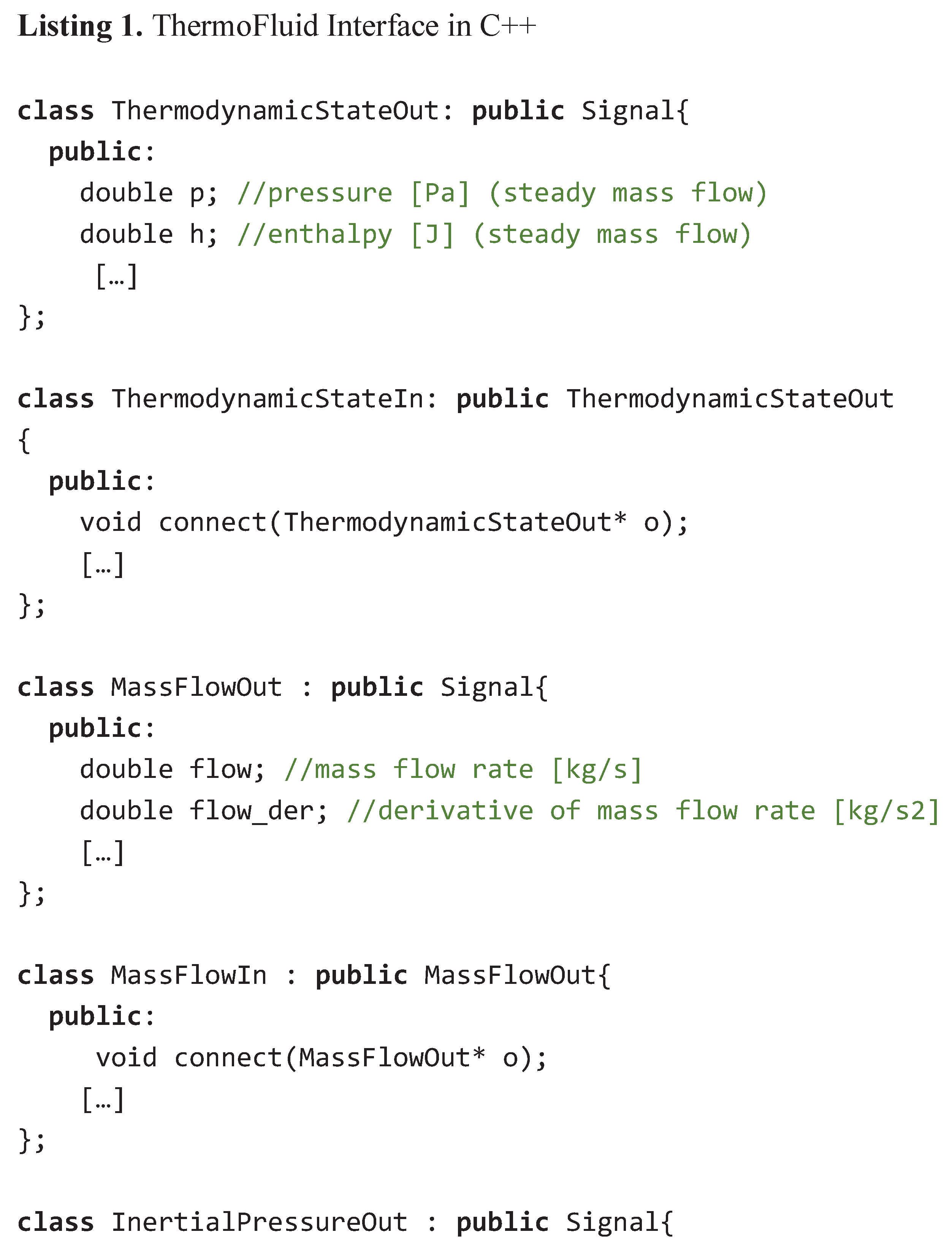
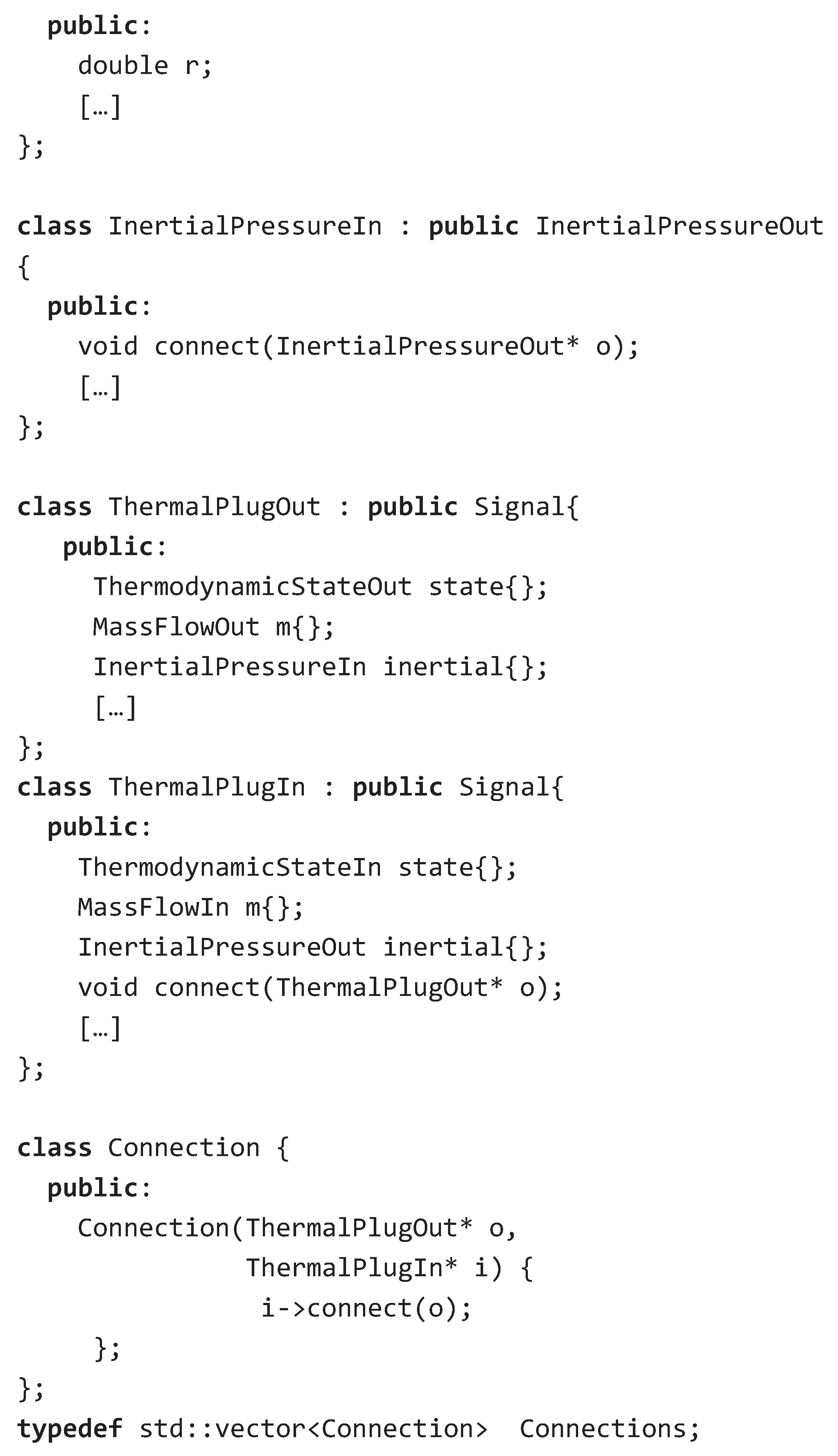
To best understand the interface, let us look at the classes ThermalPlugOut for a nominal outlet flow and at ThermalPlugIn for a nominal inlet flow first. These contain the same 3 components as the corresponding Modelica connector of the DLR ThermoFluid Stream library.
There are two notable differences however. In Modelica, inertial pressure and mass flow were not causalized signals as in the C++ implementation. Also the mass-flow signal in the C++ library consists of the mass-flow rate and its derivative. In Modelica, this is not necessary since symbolic differentiation can be applied by the Modelica compiler. Using this interface, we can now implement a component such as the pressure drop:
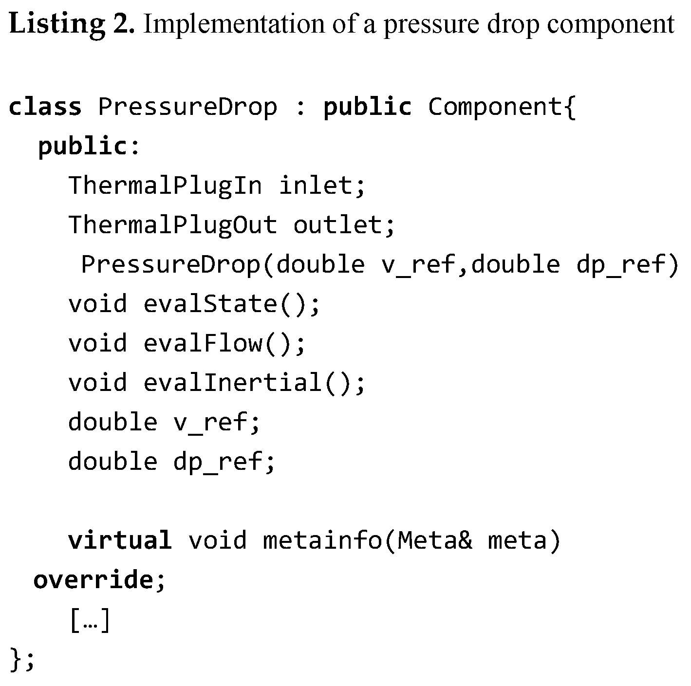
First, we declare our interface for outlet and inlet, then we have to implement three methods. The first is evalState and computes the thermodynamic state downstream:
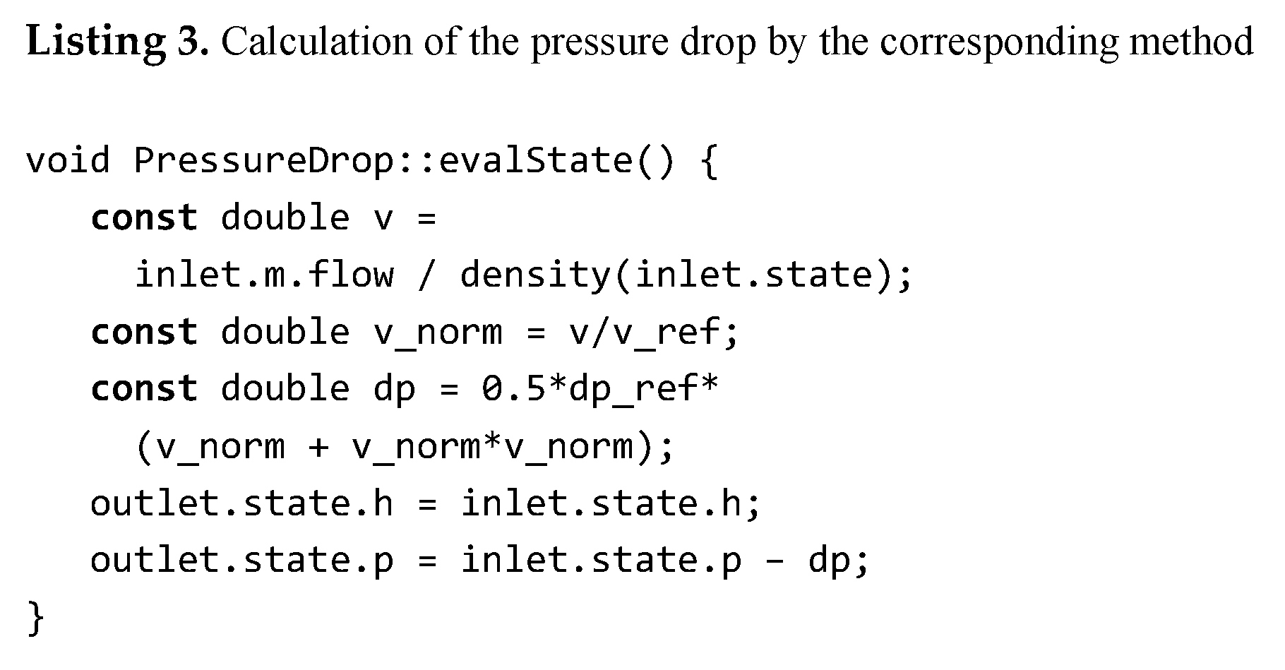
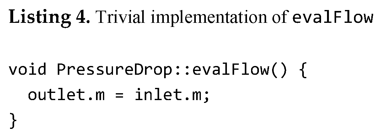
The second method is evalFlow to ensure what flows in is what flows out. However, this constraint is restated for the derivative. This is because the dummy derivative method is applied on the component level.
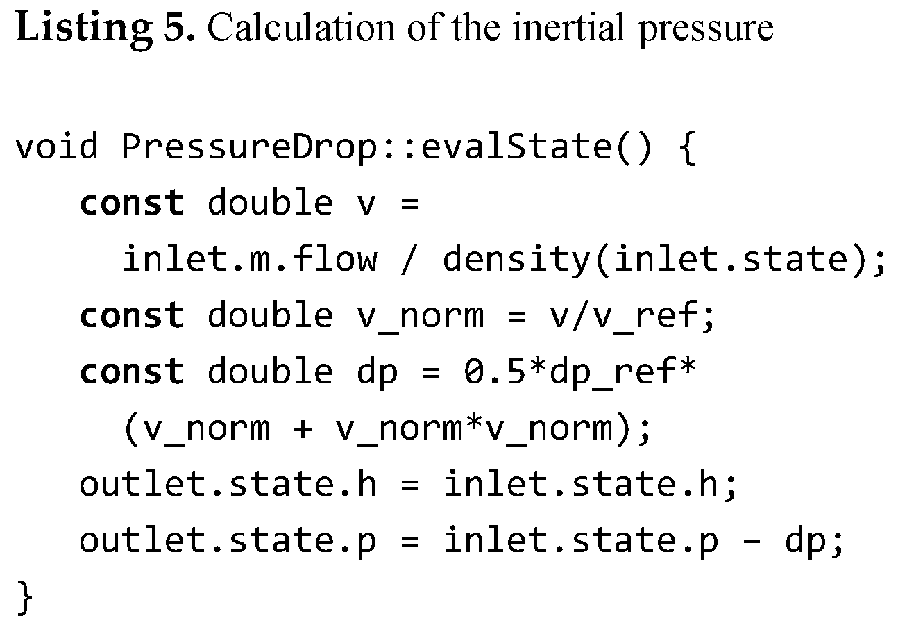
The third one is evalInertia that implements the law for the inertance as in the ThermoFluid Stream Library.
In similar manner the other components of our introductory example can be implemented. Each of these components declares its interfaces, defines and implements methods representing the computational blocks. For all these components, meta-information must be collected by a dedicated virtual method to register state and tearing variables as well as to track the signal dependence of the computing blocks. Finally, we can compose the introductory example of section 2 and 3 directly in C++:
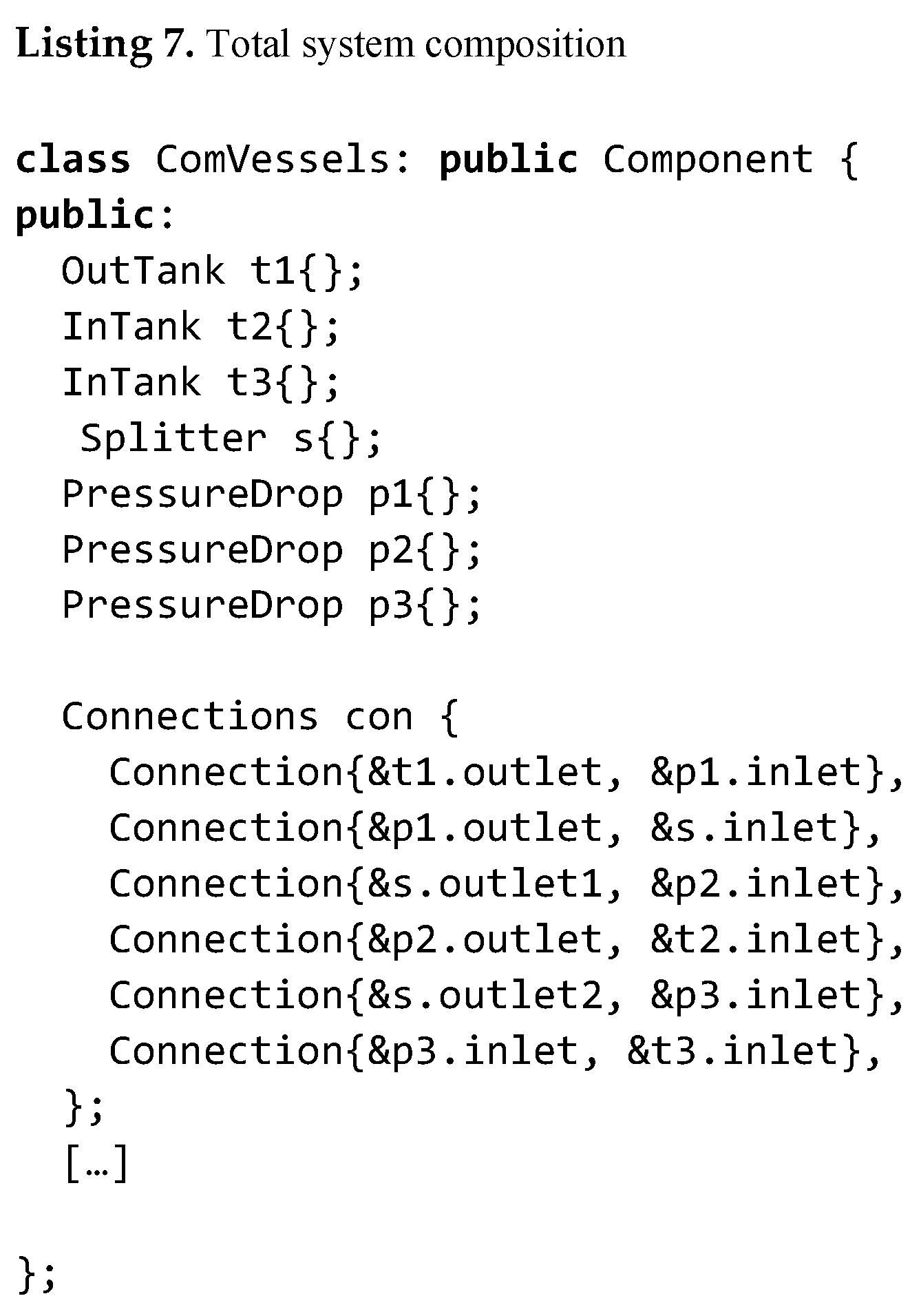
Regarding that C++ is a statically compiled imperative general-purpose language, the final result is astonishingly close to what a modeler is used to from a domain specific language like Modelica.
When an instance of the class is coupled to a simulator, the meta information of all its computational methods is collected as well as the structural information regarding the signals, the states and the tearing variables for the linear equation system. Then the methods are put into right order for complete or partial model evaluation. The full model evaluation is thus simply a list of method calls that are called in their respective order. The linear implicit system defined by is reconstructed by using the tearing variables and their residuals for probing. This requires a number of partial model evaluations.
This also means that all component code is statically compiled but the total system composition is performed at run-time. Advanced tasks such as variable structure systems would thus be comparably easy to achieve.
This is also the purpose of this code demonstration. It is not suggesting that we should use C++ as modeling language like Modelica but to highlight that for a certain class of models the object-oriented modeling code could (and maybe should) be translated to object-oriented imperative code that can be statically compiled even before total system composition. This would avoid the flattening of all equations before code generation and help to overcome many limitations of current Modelica compilers with respect to scalability.
7. Conclusions
This paper started with a very fundamental consideration about the solvability of general formulations for classic physical systems, then presented a new interface for the object-oriented modeling and ended up showing a simplified generation of simulation code potentially suitable to handle challenges such as large-scale system simulation or variable structure systems. It is quite remarkable that the two derived criteria for handling the kinetic energy have such practical consequences for object-oriented modeling.
Indeed, that a more restrictive class of modeling enables a simpler compilation scheme is neither new nor surprising. The same can be said about the many conventional signal-based modeling schemes or simple modeling schemes as Forrester’s System Dynamics [21]. Typically, the disadvantage is that the easier generation of simulation code has to be paid by an inferior modeling approach and indeed modeling complex mechanics or thermofluid streams is painful when using purely signal-based approaches (nevertheless this pain has been taken in industrial practice all too often).
The remarkable thing about the LIED approach is that a simulation engineer has a simple scheme for code generation but can also conveniently model both mechanics and thermo-fluid streams in a very robust manner. The corresponding Modelica Libraries prove this [15,16]. Both application domains are known to be rather difficult but LIED can even be applied to the challenging parts of these fields such as handling stiff contact mechanics or elaborate by-passes in complex thermal architectures. It is yet unclear for what other domains LIED is an attractive choice.
Figure 11 attempts to qualitatively depict the trade-off between computational complexity and algorithmic complexity. LIED forms a very exposed point on a hypothetical Pareto front. This means that for a large number of applications it is a very attractive choice.
It might be not unimportant to note that the actual discovery of the LIED approach happened not the way it was presented in this paper. Rather the opposite reflects reality: practical applications came first; generalization and theory came second. The approach was simply born out of the necessity (or desperation) to find robust solutions for aircraft environmental control systems and to handle gripping of stiff objects with robots.
For this paper, this means that most of its statements are to be regarded as empirical. For some specific LIED systems, formal statements on structure and solvability could be made [14] but in general, the statements on suitable system composition and code generation are merely observations from simulation practice and test implementations. Further solidification of the theoretical understanding is needed. This is a call to ourselves but also an invitation to the research community.
As the question marks in Table 3 indicate, there remains an open question whether the LIED approach can also be successfully applied for electrical systems so that it is of practical value. Clearly, kinetic energy plays a far less important role for electrical systems, also the formulation of potential energy requires a generalized form. Hence, the reasoning of this paper cannot be directly converted. Maybe extensions are needed, maybe it is infeasible? Again, this open question is an invitation to the research community.
The primary motivation of this paper remains to raise awareness on this class of models and the possibilities it enables for the generation of simulation code. Although it states mostly observations, these observations seem valuable to share.
Funding
This research received no external funding.
Acknowledgments
The author wants to thank Prof. Martin Otter for additional background on Hamilton’s principle and a review of the LIED definition. Furthermore the author expresses his gratitude to Modelica Community and the many though-provoking and encouraging discussions in the aftermath in the context of this research.
Conflicts of Interest
The authors declare no conflicts of interest.
References
- P. Fritzson, Principles of Object-Oriented Modeling and Simulation with Modelica 3.3, 2nd ed., IEEE Press, Piscataway, New Jersey, 2014, pp. 1256.
- Cellier, F.E. (1991) Continuous System Modeling. Springer Verlag New York. 755p.
- Karnopp, D.C., D.L. Margolis, R.C. Rosenberg (2006), System Dynamics: Modeling and Simulation of Mechatronic Systems. 4th Edition, John Wiley&Sons, New York, 576p.
- Zimmer, D. (2010), Equation-Based Modeling of Variable Structure Systems PhD Dissertation, ETH Zürich, 219 pages.
- Braun, Willi et al. “Solving large-scale Modelica models: new approaches and experimental results using OpenModelica.” International Modelica Conference (2017). [CrossRef]
- Fritzson, Peter A. et al. “The OpenModelica Integrated Modeling, Simulation, and Optimization Environment.” Proceedings of The American Modelica Conference 2018, October 9-10, Somberg Conference Center, Cambridge MA, USA (2019).
- Feynman, Richard P. (1942). Laurie M. Brown (ed.). The Principle of Least Action in Quantum Mechanics. PhD Dissertation, Princeton University. World Scientific (with title "Feynman's Thesis: a New Approach to Quantum Theory") (published 2005). ISBN 978-981-256-380-4.
- Georg Hamel, Theoretische Mechanik 1949 (Reprint 1978).
- Torby, Bruce (1984). "Energy Methods". Advanced Dynamics for Engineers. HRW Series in Mechanical Engineering. United States of America: CBS College Publishing. ISBN 0-03-063366-4.
- Landau LD and Lifshitz EM (1976) Mechanics, 3rd. ed., Pergamon Press. ISBN 0-08-021022-8.
- Pennrose, R., The Road to Reality. Vintage Books, New York, 2004.
- B.S. Massey, Mechanics of Fluids, Chapman & Hall. ISBN 0-412-34280-4, 1989.
- C.E. Brennen, Internet Book on Fluid Dynamics, Dankat Publishing, Pasadena, California, USA, 2015.
- Zimmer, D. (2020), Robust Object-Oriented Formulation of Directed Thermofluid Stream Networks . Mathematical and Computer Modelling of Dynamic Systems, Vol 26, Issue 3. [CrossRef]
- Zimmer, D., N. Weber, M. Meißner (2022) The DLR ThermoFluid Stream Library. MDPI Electronics - Special Issue.
- Zimmer, D., C. Oldemeyer (2023). “Introducing Dialectic Mechanics”. Proceedings of the 15th International Modelica Conference, Aachen.
- Oldemeyer, C., D. Zimmer (2023). “Dialectic Mechanics: Extension for Hard Real-time Simulation”. Proceedings of the 15th International Modelica Conference, Aachen. [CrossRef]
- Mattsson, S.E., Gustaf Söderlind (1993). “Index Reduction in Differential-Algebraic Equations Using Dummy Derivatives” In: SIAM Journal on Scientific Computing 1993 14:3, 677-692. [CrossRef]
- Pantelides, C. The consistent initialization of differential-algebraic systems. SIAM J. Sci. Statist. Comput. 1988, 9, 213–231. [Google Scholar] [CrossRef]
- Sven Erik Mattsson, H. Olsson, H. Elmqvist (2000) “Dynamic Selection of States in Dymola”. Proceedings of Modelica Workshop 2000.
- Junglas, P. (2016), Causality of System Dynamics Diagrams, SNE Simulation Notes Europe 26/3, 147-154.
Figure 1.
This topological map illustrates the complexity of the action over time (x-axis) for a straight path of constant velocity (y-axis). The potential has here been arbitrary chosen in this example and the actual values are irrelevant. Relevant is that the complexity of the action is increasing over time.
Figure 1.
This topological map illustrates the complexity of the action over time (x-axis) for a straight path of constant velocity (y-axis). The potential has here been arbitrary chosen in this example and the actual values are irrelevant. Relevant is that the complexity of the action is increasing over time.
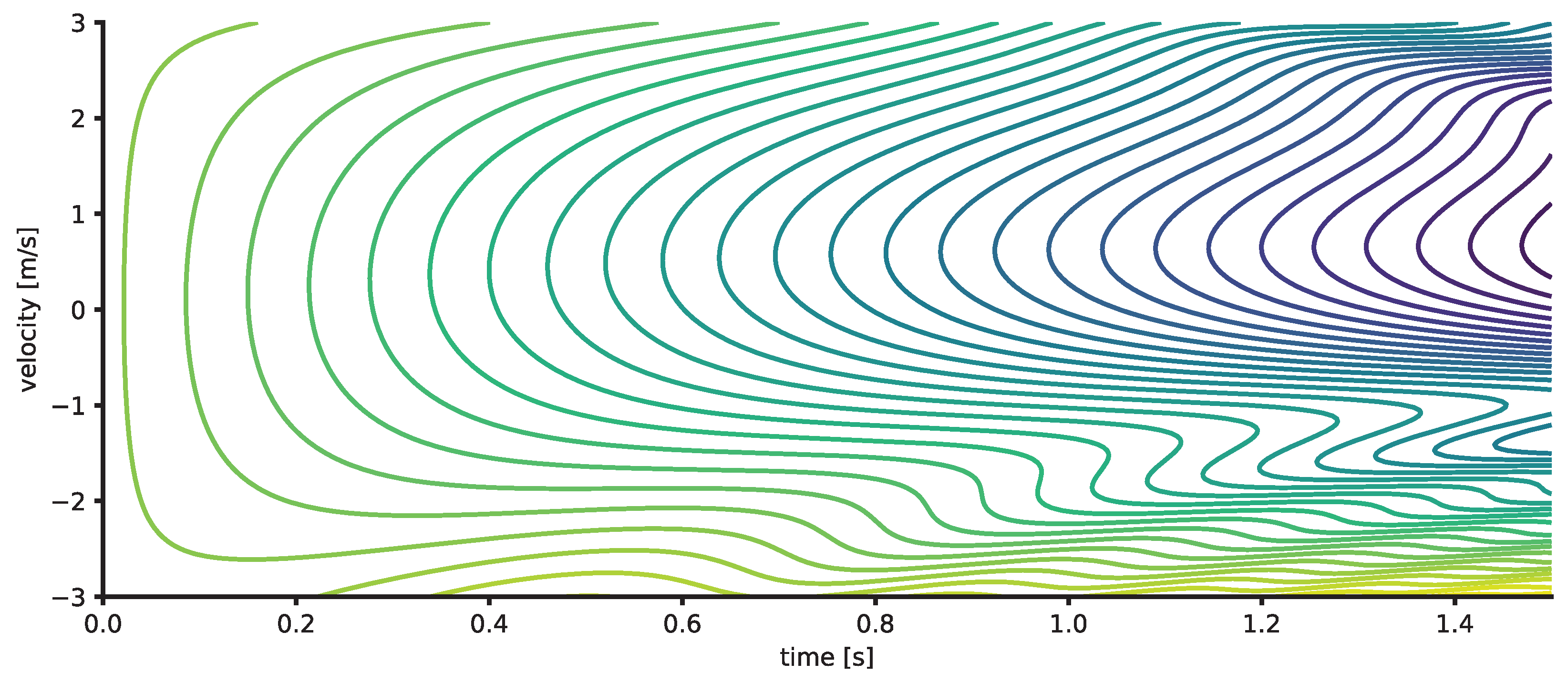
Figure 2.
This diagram represents a model of three communication vessels. Gravitational pressure is modeled at the tanks. Non-linear flow resistance is used to model the valve at the outlets. The connecting pipes are modeled using inertances and compressible volumes.
Figure 2.
This diagram represents a model of three communication vessels. Gravitational pressure is modeled at the tanks. Non-linear flow resistance is used to model the valve at the outlets. The connecting pipes are modeled using inertances and compressible volumes.
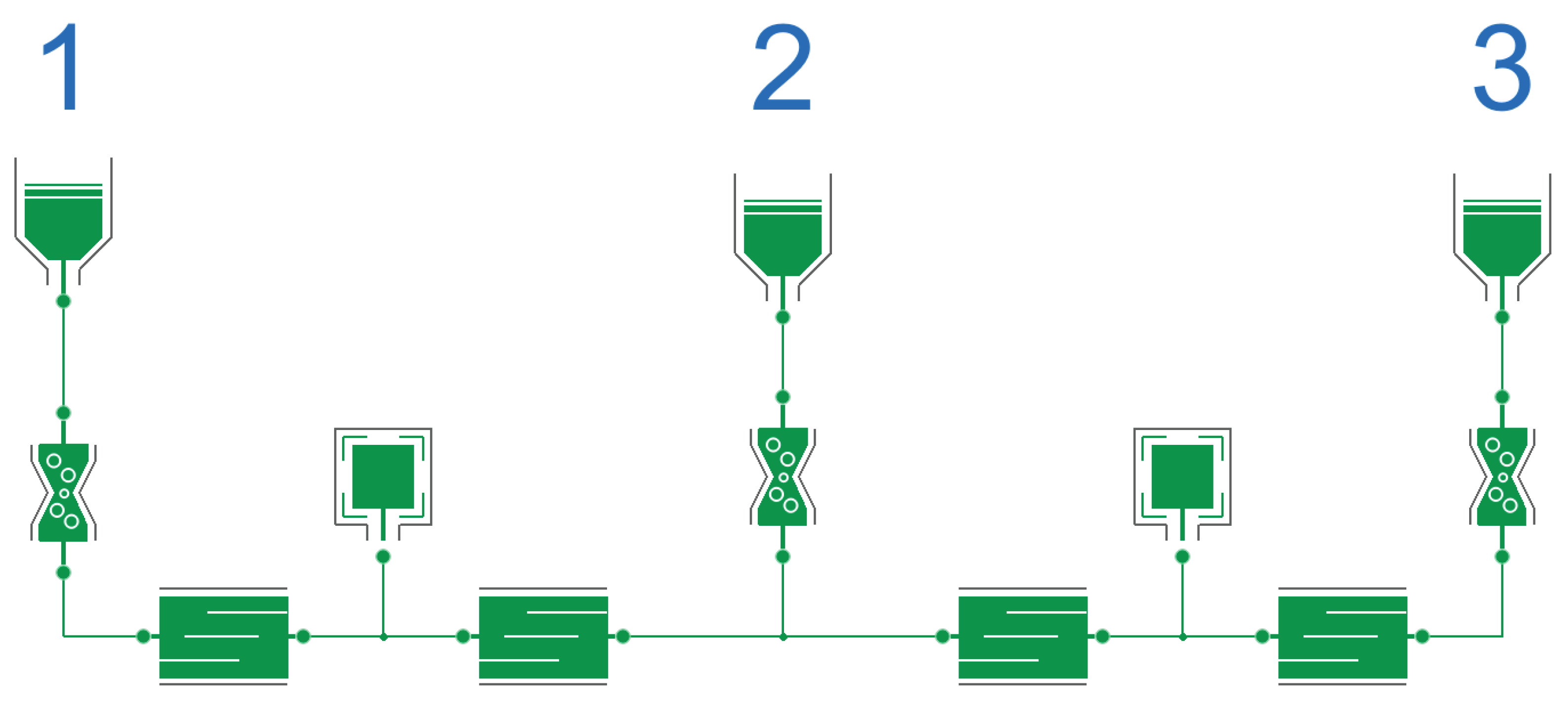
Figure 3.
Simulation result of the model of Figure 2, showing the 3 volume flows going through the tank’s orifices. A sudden change of water level is imposed to the system a time to trigger the low-frequency response.
Figure 3.
Simulation result of the model of Figure 2, showing the 3 volume flows going through the tank’s orifices. A sudden change of water level is imposed to the system a time to trigger the low-frequency response.
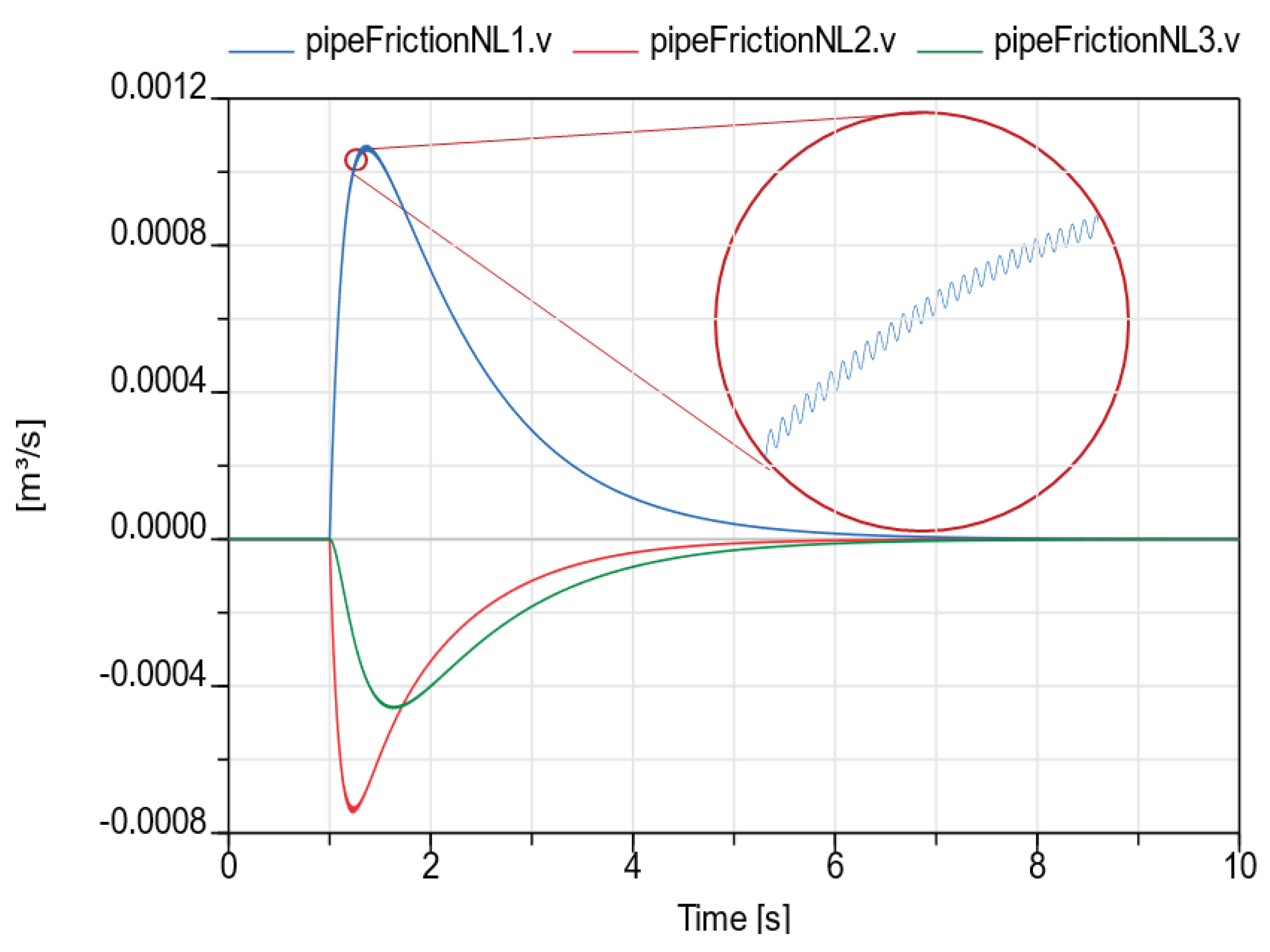
Figure 4.
Modeling 3 communicating vessels without modeling the pipe just by the gravitational pressure and the flow-resistance of the orifice. Note, that there is an algebraic non-linear equation system to determine the pressure below the valves so that all flows are in balance.
Figure 4.
Modeling 3 communicating vessels without modeling the pipe just by the gravitational pressure and the flow-resistance of the orifice. Note, that there is an algebraic non-linear equation system to determine the pressure below the valves so that all flows are in balance.
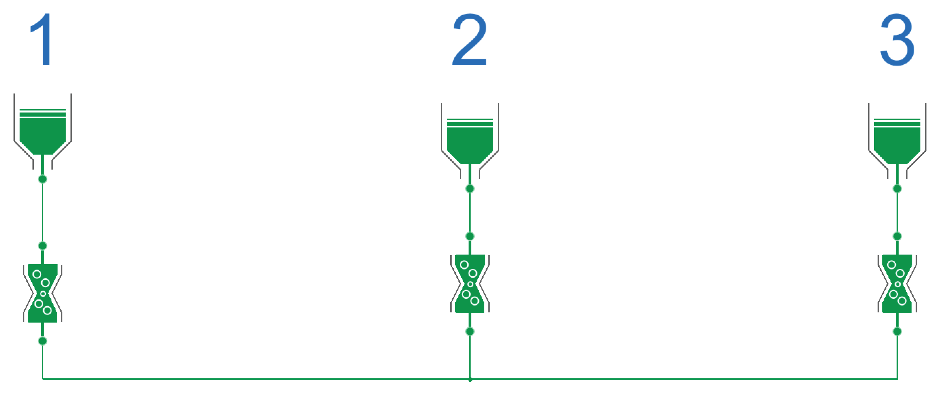
Figure 6.
For this particular model of the communicating vessels, the LIED approach has an equivalent counterpart using conventional connectors. Modeling the inertia but leaving out the compressibility does the trick here.
Figure 6.
For this particular model of the communicating vessels, the LIED approach has an equivalent counterpart using conventional connectors. Modeling the inertia but leaving out the compressibility does the trick here.
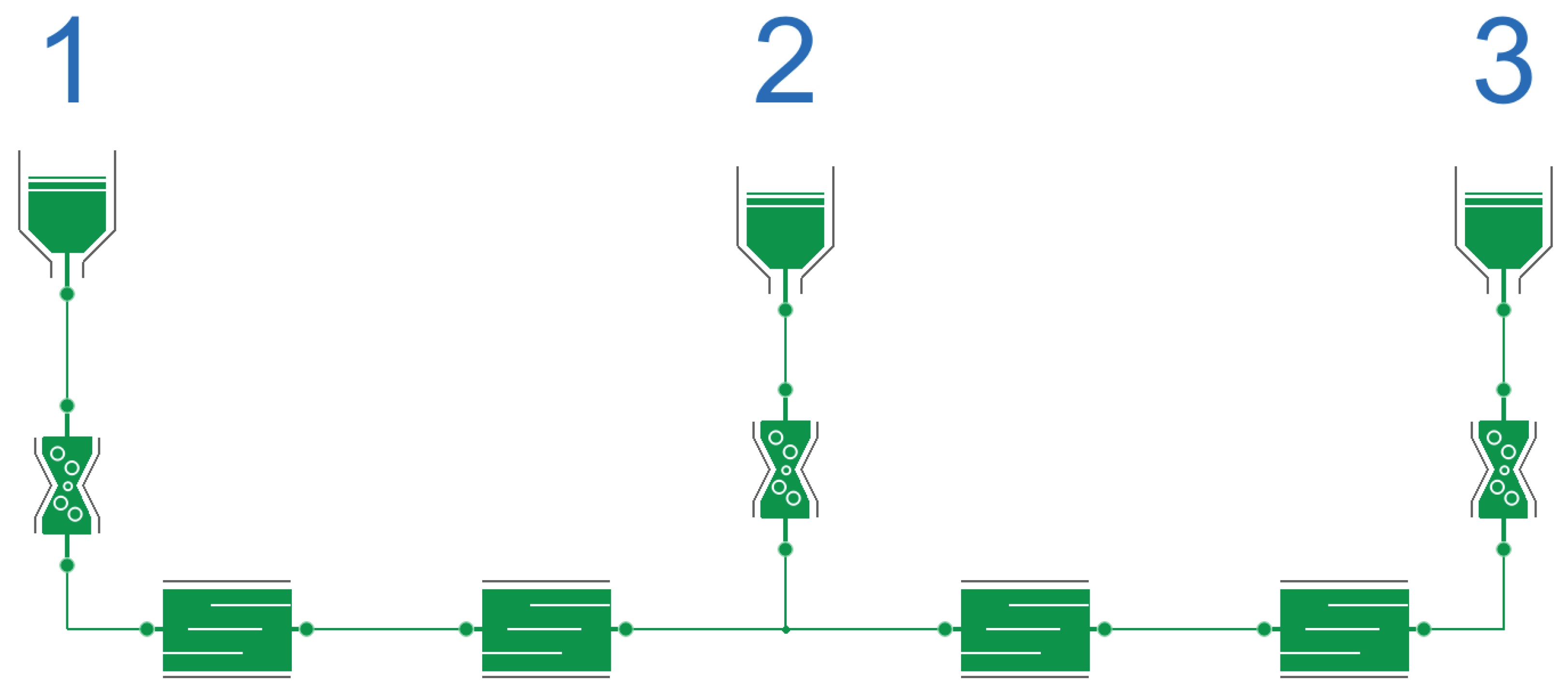
Figure 7.
Modelling the communicating vessels by the sheer exchange of potential energy.
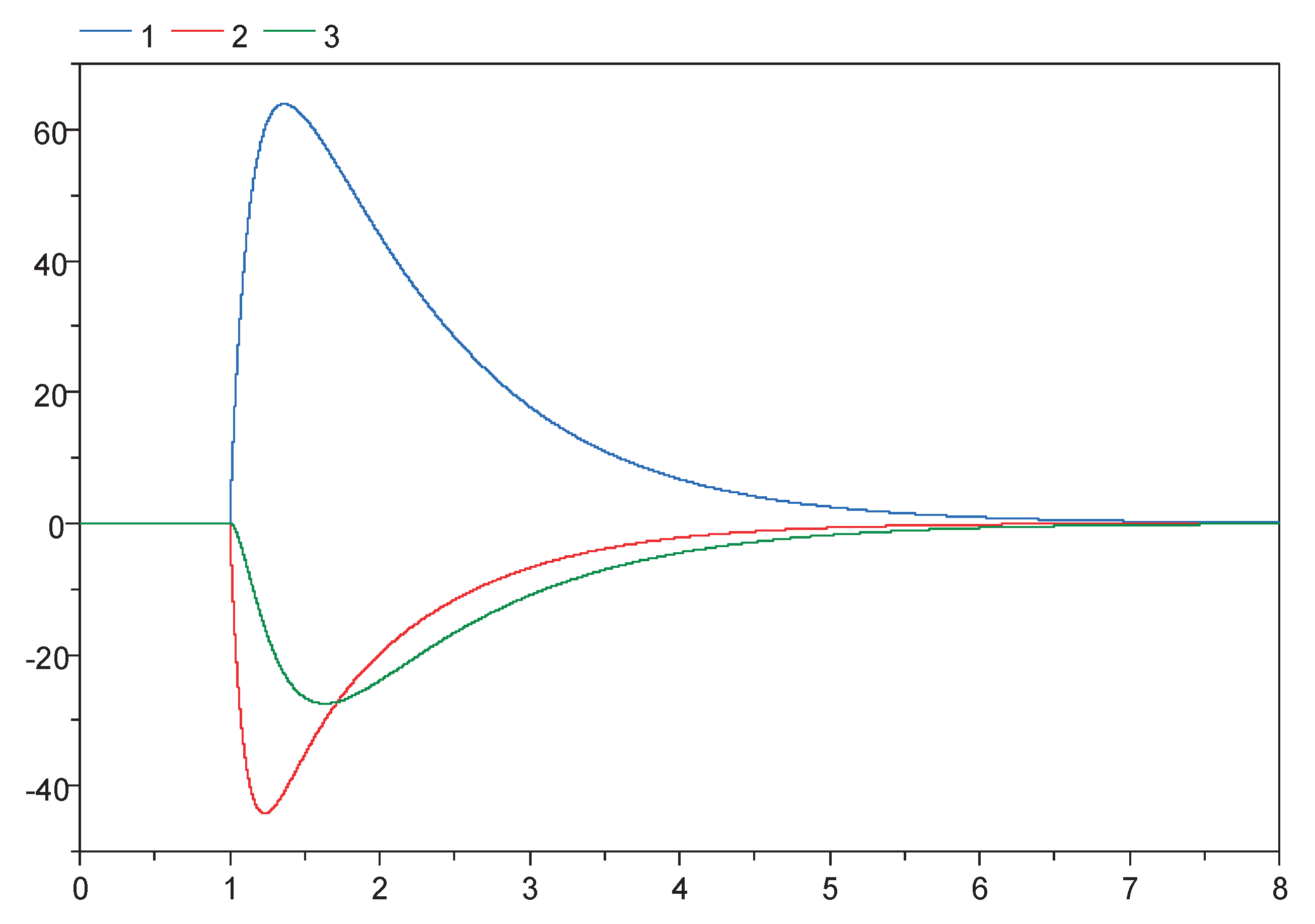
Figure 8.
Penetration depth into the left claw represented by an elasto-gap, for the choice of two different time constants, taken from [16]. Both agree on the time-averaged solution. TC of the legend represents . The dots of the blue result from a decaying high-frequent oscillation. The red line is the low frequency approximation.
Figure 8.
Penetration depth into the left claw represented by an elasto-gap, for the choice of two different time constants, taken from [16]. Both agree on the time-averaged solution. TC of the legend represents . The dots of the blue result from a decaying high-frequent oscillation. The red line is the low frequency approximation.
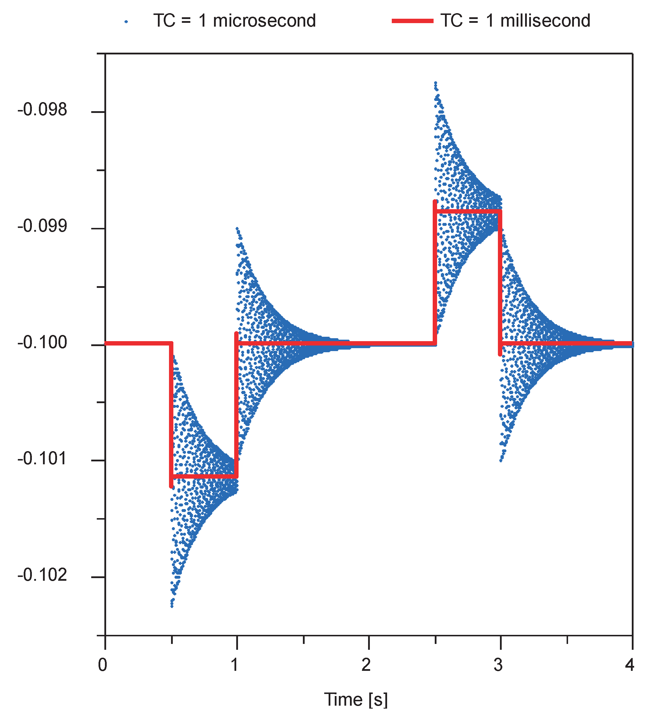
Figure 9.
Exemplary model diagram taken from [15] of the thermal architecture of an electric car. Different cooling loops, including a vapour cycle can be combined to cool the power electronics, battery and passenger compartment of the car. Certain components are marked with a star which is not part of the original diagram. The meaning of this marking is explained in section 6.
Figure 9.
Exemplary model diagram taken from [15] of the thermal architecture of an electric car. Different cooling loops, including a vapour cycle can be combined to cool the power electronics, battery and passenger compartment of the car. Certain components are marked with a star which is not part of the original diagram. The meaning of this marking is explained in section 6.
Figure 10.
Modelica Diagram (left) of a landing gear kinematic (right) using the Dialectic Mechanics library. The interface of the LIED approach leads to a nice decomposition into ideal components. Regarding the star marking, the same comment as in Figure 9 applies.
Figure 10.
Modelica Diagram (left) of a landing gear kinematic (right) using the Dialectic Mechanics library. The interface of the LIED approach leads to a nice decomposition into ideal components. Regarding the star marking, the same comment as in Figure 9 applies.
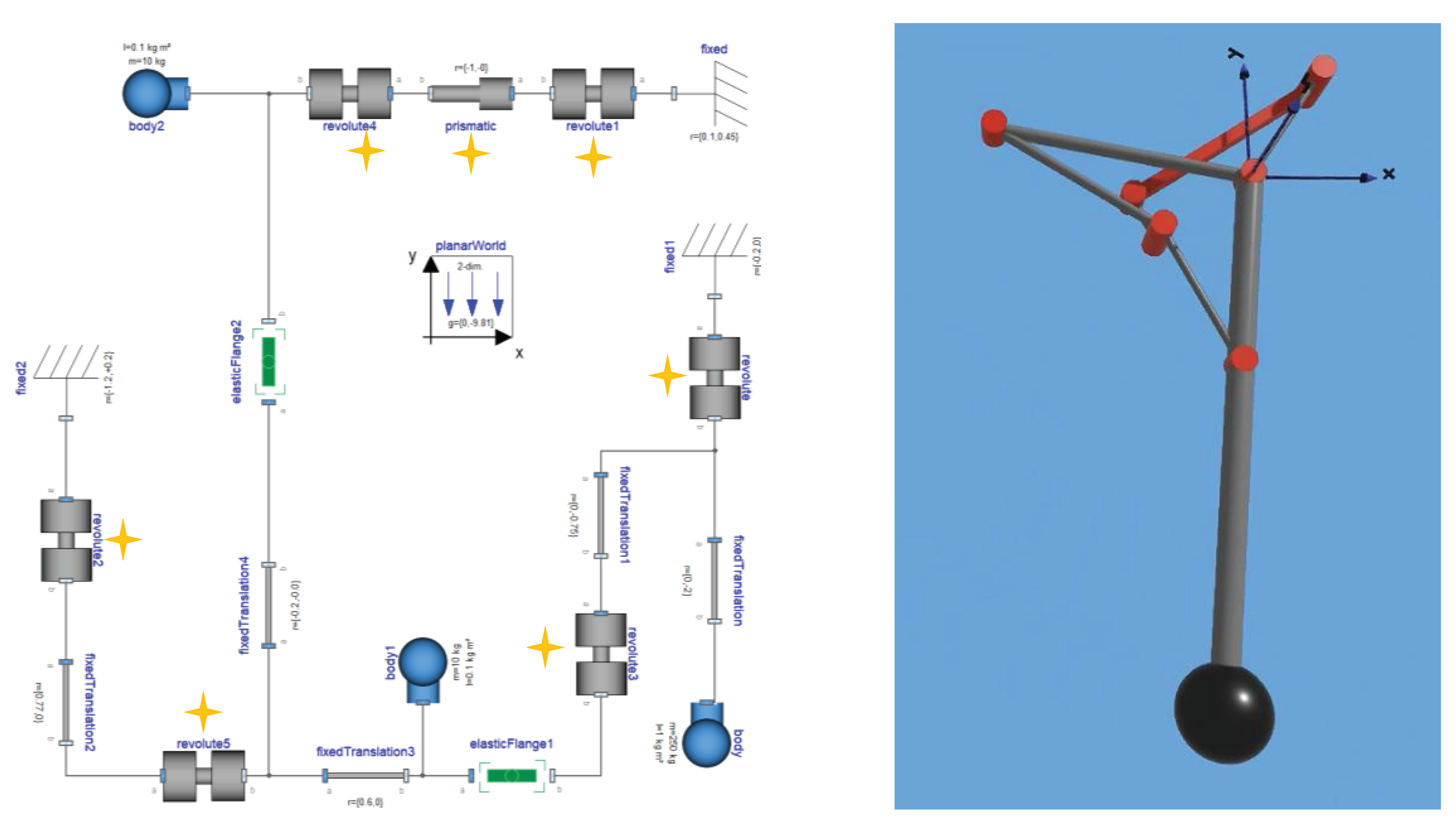
Figure 11.
Hypothetical Pareto front weighing computational complexity against algorithmic complexity for code generation. Distributed (object-oriented) DAE Systems enable a very effective compression of reality and very efficient models. The same compression is often infeasible to achieve with distributed ODE system but code is much easier to generate. LIED systems form an attractive compromise. The ultimate choice of the modeling approach depends however on the concrete application.
Figure 11.
Hypothetical Pareto front weighing computational complexity against algorithmic complexity for code generation. Distributed (object-oriented) DAE Systems enable a very effective compression of reality and very efficient models. The same compression is often infeasible to achieve with distributed ODE system but code is much easier to generate. LIED systems form an attractive compromise. The ultimate choice of the modeling approach depends however on the concrete application.
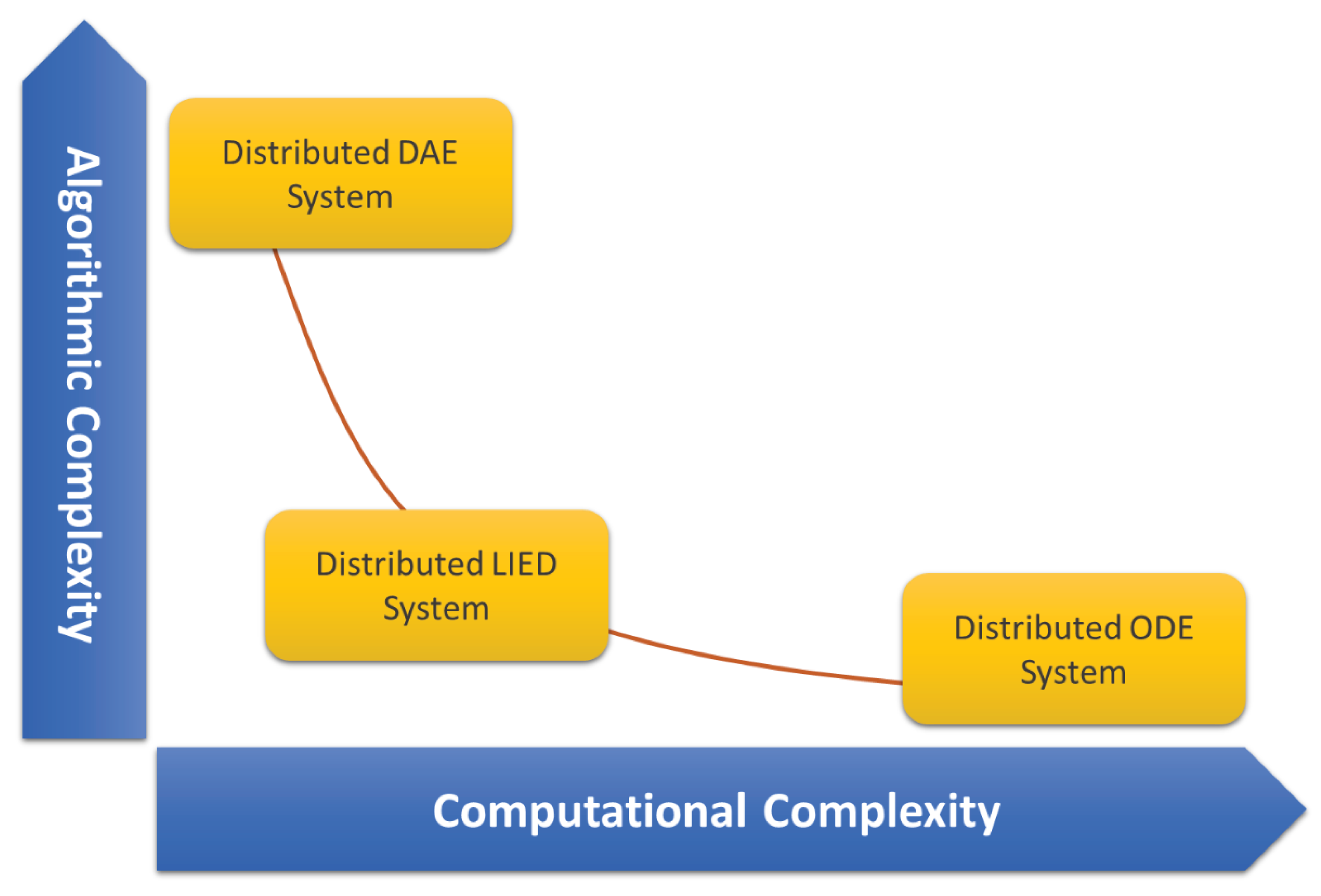

Table 1.
Connection pairs as used in the Modelica standard library
| Domain | potential variable | flow variable |
|---|---|---|
| translational mechanics | position: [m] | force: [N] |
| rotational mechanics | angle: [rad] | torque: [Nm] |
| thermofluid streams | thermodynamic state: 1 | mass-flow rate: [kg/s] |
| electrical | voltage potential: [V] | current: [A] |
1 The thermodynamic state is a tuple. Its number of elements and their units may vary depending on the medium that is modelled. For an ideal gas, one may use pressure and temperature: ([Pa], [K]).
Table 2.
Connection pairs as defined by the bond-graph methodology
| Domain | effort | flow |
|---|---|---|
| translational mechanics | force: [N] | velocity: [m/s] |
| rotational mechanics | torque: [Nm] | angular velocity: [rad/s] |
| hydraulics/pneumatics | pressure: [Pa] | Volumetric flow: [m3/s] |
| thermal | Temperature: T [K] | Entropy flow [J/Ks] |
| electrical | voltage: [V] | current: [A] |
Table 3.
Connection triplets suggested in this paper that will lead to a robustly solvable form.
| Domain | signal | potential variable | flow variable |
|---|---|---|---|
| trans. mechanics | position: [m] | velocity: [m/s] | force: [N] |
| rot. mechanics | angle: [rad] | ang. velocity: [rad/s] | torque: [Nm] |
| thermofluid str. | thermodynamic state: 1 | inertial pressure [Pa] | mass-flow rate: [kg/s] |
| electrical | ? | ? | ? |
Table 4.
Examples of components formulated based on the pairs resulting from the Hamiltonian equations. The variables forming the pair are marked in bold.
Table 4.
Examples of components formulated based on the pairs resulting from the Hamiltonian equations. The variables forming the pair are marked in bold.
| Component | Symbol | Equation |
|---|---|---|
| Fluid Inertance |  |
|
| Compressible volume |  |
|
| Tank 1 |
 ] ] |
|
| Flow resistance 2 |  |
1 is the cross-section area of the tank and the gravitational constant. 2 is a reference volume flow and is the quadratic friction coefficient.
Table 5.
The triplets as represented in the Modelica language for equation-based modeling.
| Thermofluids | Mechanics |
|---|---|
 | |
1 For each connector with an output there is also a counterpart with an input. Two sexes of connectors are thus needed. Only one is shown. The flow variable is marked in Modelica by the keyword flow. An unmarked variable is regarded as potential variable. 2 For the mechanical connector also a variant with two pairs of effort and flow is presented in [16]. This will be however discontinued in favor of the presented triple.
Disclaimer/Publisher’s Note: The statements, opinions and data contained in all publications are solely those of the individual author(s) and contributor(s) and not of MDPI and/or the editor(s). MDPI and/or the editor(s) disclaim responsibility for any injury to people or property resulting from any ideas, methods, instructions or products referred to in the content. |
© 2024 by the authors. Licensee MDPI, Basel, Switzerland. This article is an open access article distributed under the terms and conditions of the Creative Commons Attribution (CC BY) license (http://creativecommons.org/licenses/by/4.0/).
Copyright: This open access article is published under a Creative Commons CC BY 4.0 license, which permit the free download, distribution, and reuse, provided that the author and preprint are cited in any reuse.


