CCLR-DL: A Novel Statistics and Deep Learning Hybrid Method for Feature Selection and Forecasting Healthcare Demand

Guillem Hernández Guillamet; Francesc López Seguí; Josep Vidal Alaball; Beatriz López Ibáñez

doi:10.20944/preprints202403.1110.v1

Preprint

Article

CCLR-DL: A Novel Statistics and Deep Learning Hybrid Method for Feature Selection and Forecasting Healthcare Demand

This version is not peer-reviewed.

Guillem Hernández Guillamet^*

,Francesc López Seguí,

Josep Vidal Alaball,

Beatriz López Ibáñez

Guillem Hernández Guillamet^*

,Francesc López Seguí,

Josep Vidal Alaball,

Beatriz López Ibáñez

This version is not peer-reviewed.

Downloads

145

Views

179

Comments

Submitted:

18 March 2024

Posted:

22 March 2024

You are already at the latest version

Abstract

Hybrid forecasting methods have emerged as a solution surpassing the limitations of both statistical and deep learning approaches. While the first emphasize the significance of variables, they often produce worse forecasting results when compared to newer techniques. In contrast, deep learning models remain enigmatic "black boxes" in terms of interpretability, although achieving better results in forecasting. This article introduces the Comprehensive Cross-Correlation and Lagged Linear Regression Deep Learning (CCLR-DL) framework, designed to harness the best of both approaches, enhancing forecasting accuracy while retaining model interpretability through a feature selection process. CCLR-DL blens cross-correlation analysis, lagged multiple linear regression and granger's causality procedures with deep learning architectures based on LSTM. In a practical demonstration, CCLR-DL was applied to a real database of clinical visits associated to diagnoses in Catalonia, Spain (tracking a population of 6.3 million patients during 10 years). Predicting visits enables the healthcare managers to be ready for future demand shifts. Results demonstrate a consistent and substantial improvement over standalone statistical and deep learning methods when predicting healthcare demand. This hybrid approach not only showcases its efficacy but also offers a promising solution to the challenge of balancing predictive accuracy with model explicability. In this context, this work aims to design and validate a method for feature selection and forecasting of multivariate high dimensional time series datasets not only to improve prediction accuracy but also to model transparency by identifying a subset of variables that improve predictions and G-cause the target variable.

Keywords:

Deep learning

;

explainability

;

feature selection

;

Granger causality

;

health demand modelling

;

LSTM

;

multivariate time-series forecasting

Subject:

Computer Science and Mathematics - Artificial Intelligence and Machine Learning

This preprints belongs to the Topic

Artificial Intelligence in Public Health: Current Trends and Future Possibilities

1. Introduction

Predicting future demand has been a fundamental challenge in various domains, driven by the need to anticipate resource consumption and optimize distribution strategies. This is a particular challenge in the healthcare sector. Many developed countries face a shortage of healthcare professionals, an aging population, chronic underfunding in public healthcare systems, operational strain, talent attrition, and long waiting lists. This complex landscape was further disrupted by the COVID-19 pandemic and highlights the importance of effective planning by government agencies and healthcare bodies across the world [1,2,3]. In Catalonia (Spain) the pandemic has not only stretched the healthcare system to its limit but also altered its traditional operation [4,5]. In this context, the capacity to anticipate future healthcare demand holds significant value. However, the importance of forecasting in healthcare transcends mere demand prediction; it extends to the critical domain of predicting the underlying reasons and understanding for patient consultations, specifically the diagnoses associated with medical visits. Such predictive insights can help institutions to transition to a more versatile and responsive healthcare ecosystem. Forecasting clinical demand has previously been studied via statistical means using models such as ARIMA, Seasonal ARIMA, Moving Average and decomposition models [6]. These models are based on the serial correlation of the target time series to predict its future values. The univariate nature of these models creates a suitable framework for applying these algorithms to epidemiological visits, where future values are influenced by past values. However, these models have limitations in terms of forecasting accuracy due to their parametric linear nature; and the univariate character of the models may result in missing information from other temporal processes that could improve forecasting. To overcome these limitations, first statistical models such as Vector Autoregression (VAR) and finally Deep Learning (DL) based models enhanced predictivity power with non-linear formulations, also taking into account multivariate data [7]. However, these models are considered opaque in terms of explainability [8]. The development of post-hoc explainability tools to overcome such limitations, such as Shap values [9], partially solved the issues but still rely on the expertise of the developer and are not as well-defined for time series models. In this sense, the recent definition of hybrid models, which combine statistical and DL approaches, captures the linear and non-linear behavior of time series in healthcare visits, enhancing accuracy. However, they also tend to struggle in identifying the key predictors and the subsequent relationship with the target time series in highly dimensional datasets. In such datasets, best results are typically achieved only using past values of the target time series, assuming the seasonality effect. In response to these challenges, this paper introduces the Comprehensive Cross-Correlation and Lagged Linear Regression Deep Learning (CCLR-DL) framework for forecasting time series data in high dimensional multivariate datasets. The method is positioned at the confluence of statistics and deep learning techniques. While designed to improve the accuracy of predictions; it also aims to uncover the underlying causal reasons underlying complex healthcare demand patterns.

1.1. Contributions

The contribution of this work can be summarized in the following points:

CCLR-DL, a hybrid model based on conventional statistical techniques and deep learning. It not only demonstrates its effectiveness but also provides a promising solution to the challenge of balancing predictive accuracy with model transparency.
CCLR-DL is capable of selecting a subset of predictors that achieve better results than using other feature selection strategies, that way identifying predictors that GC the variable.
The model forecasts the number of clinical visits linked to diagnoses, and therefore clinical demand, potentially helping policy making and healthcare planning.

The rest of this article is organized as follows. In Section 2, related research is reviewed. In Section 3 we provide a detailed description of the proposed framework architecture and its different phases. In Section 4 experimental results are presented. Discussion of the work is conducted in Section 5. Finally, conclusions are drawn in Section 6. Appendix A defines the notation used in the methodological part. Other results can be shown in Appendix B.

2. Literature review

Mitigating future uncertainty to refine decision-making is a pivotal aspect in diverse fields, processes, and businesses. The temporal dimension is intrinsic to many prediction challenges, requiring the extrapolation of time series data. Precise forecasting not only enables effective planning, optimization, and risk identification but also opens avenues for seizing opportunities. Consequently, accurate time series forecasting has evolved into a cornerstone of data science, prompting substantial efforts to advance and refine forecasting methods. In this context, initial proposals were based on statistical models. This encompasses exponential smoothing, seasonal, ARIMA, and state space models, among others [6]. These methods are based on their prescription of the underlying data-generating process, assuming the structural components of the series and the correlation of historical observations. These models require a small number of parameters and can handle cases with limited historical observations. In recent years, methods based on DL have surpassed statistical approaches, particularly in multivariate datasets and for longer forecast horizons. These methods can capture both short-term dependencies among variables and discover long-term patterns [10]. In the healthcare context, there is literature focused on forecasting demand. An area of significant research interest involves predicting emergency attendance for precise resource planning. Studies such as [11], employ LR analysis to link emergency departments with specific resources, highlighting the significant enhancements simple tools can bring to healthcare systems in terms of resource management. The work by [12] use RNN to predict patient visits using previous diagnosing information. Some predict visits using DL, while others forecast unplanned visits for diabetic patients [13]. Numerous studies predict epidemiological visits, like flu outbreaks [14]. Particularly within the context of the COVID-19 pandemic, there has been a notable increase in research efforts due to the availability of datasets. In the research conducted by [15], LSTM models outperformed statistical models such as ARIMA and the Nonlinear Autoregression Neural Network (NARNN) when applied to modeling the spread of the pandemic in countries like Germany, France, Belgium, and Denmark [16]. In [17], various LSTM models (e.g., Bi-LSTM, ed-LSTM) were employed for short-term forecasting in India. The study suggests that including external factors such as population density, travel logistics, or sociodemographic data could enhance predictions. Other works also employ standard implementations of LSTM on Canadian databases [18]. In [19], various models were compared, including LSTM, Bi-LSTM, GRU, SVR, and ARIMA. Bi-LSTM performed best with lower Mean Absolute Error (MAE) and Root Mean Square Error (RMSE). In multivariate studies, climate variables are used for improving COVID-19 outbreak predictions [20,21,22,23]. These methods, despite obtaining promising results, focus on improving prediction and do not aim to discover the underlying relationship of variables, select predictors, and enhance explainability in the models as we are proposing in the present work.

Hybrid models that integrate statistical and deep learning methods, as the one proposed in this work, have been previously proposed achieving promising results. In [24], a combination of Multiple Linear Regression (MLR) and Artificial Neural Networks (ANN) is used to address the complexity of emergency attendance in a tourist area, where significant seasonal variations occur. In [25], the Multivariate Exponential Smoothing Recurrent Neural Network (MES-RNN) framework is proposed to improve forecasts. This approach draws from the principles outlined in the works of [26,27]. They expand upon earlier research in multivariate time series exponential smoothing to create structural models that can generate optimal forecasts for individual data series. The MES-RNN method demonstrates consistent results when forecasting COVID-19 outbreaks in aggregated disease morbidity datasets, outperforming purely statistical or deep learning models. In the study by [28] a hybrid model combining linear regression models, often referred to as autoregression-LR, or ARIMA (Auto-Regressive Integrated Moving Average), with nonlinear models based on deep belief networks (DBN) is presented. This blending is employed to effectively capture both linear and nonlinear patterns within time series data, demonstrating that these propositions enhance performance when compared to purely linear or nonlinear models; in contrast to the aforementioned approaches, our CCLR-DL method not only seeks improvement in deep learning forecasting through statistical techniques but also employs these statistical methods in conjunction with Granger causality (GC) for feature selection. This approach aims to select the most influential predictors while enhancing the transparency of the model.

The need to eliminate non-informational variables in the dataset that can worsen the forecasting and the need to understand the underlying relationships between features in multivariate contexts, create an ideal environment for applying feature selection strategies. The gold-standard feature selection methods for enhancing explainability in DL is based on the post-hoc Shapley Additive Explanations (SHAP) method, introduced in [9]. While the exact computation of Shapley values is computationally challenging, the innovation that SHAP methods bring is that the explanation model is represented as an additive feature attribution method, a linear model. It is considered an agnostic post-hoc method since it is used as a feature importance technique after the training of any model. SHAP method has a limitation based on the need of a strategy for selecting the number of predictors, usually based on a pre-established threshold. Another method of dimensionality reduction widely used in multivariate time-series databases is GC [29]. In the work of [30], a dimensionality reduction algorithm is proposed for multivariate time series datasets, which can effectively extract the most significant and discriminative input features for output predictions. In [31], a variant of RNN known as the Echo State Network (ESN) leverages GC to learn nonlinear models for time series classification. Other studies have employed GC as a feature selection method to enhance model interpretability and improve forecasting [32,33]. Our CCLR-DL methodology blends Lagged Multiple regression models and Granger causality to extract significant predictors. This serves a dual purpose: firstly, it refines the feature selection strategy considering lags for identifying predictors, and secondly, it enhances the forecasting accuracy of Deep Learning (DL) models. The objective is to create an autonomous method to select predictors in multivariate time series data and enhance model explicability.

The results of these studies demonstrate the potential of hybrid strategies for predicting time series in both univariate and multivariate scenarios. Our proposal aims to develop a model that can be used in a multivariate temporal database without relying on specific domain knowledge, assuming that predictors are present in the dataset. The method is based on a feature selection strategy based on statistical procedures for both enhancing explainability and improving forecasting accuracy of DL models.

3. Methods

The CCLR-DL algorithm is a method for time series forecasting in multivariate high-dimensional datasets. The method ensembles a feature selection strategy based on Lagged MLR and GC [29] with DL for enhancing forecasting accuracy and increase explainability. The proposed framework consists of three separate phases (see Figure 1). The first phase, based on statistical techniques, utilizes cross-correlation analysis to select an uncorrelated subset of predictors. Lagged multiple linear regression models are developed to predict the target variable. The forward stepwise estimation method is used to iteratively introduce and assess predictors. The second phase ensures all predictors G-cause the target time series and leads to a form of causality feature selection for the predefined lagging time. This layer not only refines the feature selection procedure but is also devoted to extracting knowledge in the predictors set, assessing which is the best interval relation between predictors and target time series (first and second phase form the feature selection procedure). The third phase of the algorithm employs the subset of predictors that effectively G-causes the target time series for forecasting. It entails training multiple DL architectures and selecting the most suitable one for predicting the target variable for different parametrizations.

The input of the procedure is a temporal matrix M. Each feature of the matrix represents the time series of a diagnosis

d_{i}

that belongs to a set of diagnoses

D = d_{1}, \dots, d_{N}

and a fixed time period

T = t_{1}, \dots, t_{L}

. Matrix has dimension

M = D x T

, where each cell

d_{i j} \in M

corresponds to the number of occurrences of diagnosis

d_{i}

on time-step

t_{j}

. To set up the procedure it is also mandatory to identify the target diagnoses time-series to forecast

d_{g} \in D

. The lagging regression phase selects a subset of predictors

P \subseteq D - {d_{g}}

and the G-causal phase refines the subset obtaining

A \subseteq P \subseteq D - {d_{g}}

. This matrix is later transformed and used to train the DL phase (see Figure 1).

3.1. Lagging Regression Phase

This phase represents the first part of the feature selection strategy. Based on linear regression models, it defines a lagging parameter to enable the generation of future regressions. The model aims to reduce the database of potential predictors to initially an uncorrelated subset and ultimately to a subset that best allows regression of the target time series for a lagging time. The model automates the process of predictor selection and employs a feed-forward selection strategy with systematic vigilance to select the best subset of features. Figure 2 visualizes the process of lagging MLR model generation process in the phase.

First, Pearson’s correlation coefficients

r_{i j}

are calculated to address collinearity between pairs of predictors

d_{i}

and

d_{j}

in the predictor set

D - {d_{g}}

[34]. Next the t-statistic

T S_{i j}

is determined according to Equation (1), and if significance (

p - v a l u e < . 1

), pairs of variables are considered prone to producing multicollinearity. The Variance Inflation Factor (VIF), as per Equation (2), is employed to assess the degree of collinearity. Parameter

c_{j}

signifies the coefficient of determination of variable

d_{i}

, regressed on the remaining set of predictors. The algorithm iteratively removes variables with the highest degree of collinearity until a set of potential predictors

Δ \subseteq D - {d_{g}}

reaches a maximum collinearity threshold of

m a x (V I F) = 20

, as in literature, assuming collinearity to be nonsignificant [35].

All variables within

Δ

are candidates for predicting our target variable

d_{g}

, which we aim to forecast at time t using the minimal set of predictors

P \subseteq Δ \subseteq D - {d_{g}}

. For this purpose, we apply a MLR model following Equation (3), where

t \in L

;

α_{0}

represents the constant coefficient of the model;

α_{i j}

denotes the regression coefficient of predictor

d_{i} \in P

at time j; and

τ < L

represents the applied lag value. Note that the lag value can take on the value 0, thereby predicting the target variable using variables from the same day or higher values if willing to predict future timesteps.

T S_{i j} = \frac{r_{i j} \sqrt{L - 2}}{\sqrt{1 - r_{i j}^{2}}}

(1)

V I F_{j} = \frac{1}{1 - c_{j}^{2}}

(2)

m o d e l (d_{g}, P, t, τ) = α_{0} + \sum_{i \in [1, | Δ |]} \sum_{j \in [t - τ, t - 1]} α_{i j} * d_{i j}

(3)

To select predictors, the model employs a forward stepwise estimation method (see Algorithm 1). Variables forming P are selected based on their highest correlation with the target variable

d_{g}

, and both are fitted to a linear regression model (as per Equation (3)). p represents the number of predictors used in each model. The adjusted coefficient of determination

R^{2}

is used to assess the goodness of fit, determining the percentage of variation explained by the added predictor relative to the baseline model. Predictors are added iteratively and evaluated by recalculating

R^{2}

. The F-test statistic (see Equation (4)) is used to determine whether the addition of new predictors produces a significant improvement in the forecasting model. Subscripts 1 and 2 correspond to models with the new predictor removed (

p_{1}

) or added (

p_{2}

), respectively. The variables

S S R

and

S S E

refer to the Sum of Squares error due to Regression (the variability explained by the regression) and the Sum of Squares error due to Error (the variability not explained by the regression) of the model. The significance value indicated by the F-test statistic (p-value ≥ .1) means the model significantly improves with the addition of the new predictor. Sometimes, due to the forward stepwise estimation strategy, it may be observed that the addition of one predictor does not demonstrate significance, but adding the next one does. For this reason, the algorithm allows for up to 3 iterations to exceed the p-value. Among all the models computed, the model with the best Mean Absolute Percentage Error (MAPE) is selected. In case of a tie, the model with the fewer number of predictors is preferred. The predictors of the best model are the selected features forming P.

Algorithm 1 Lagged-MLR predictors selection

Require:: $d_{g}, Δ = {d_{1}, \dots, d_{| Δ |}}, τ, t$
Ensure:: $P \subset Δ$
1:: $l i s t_o f_m o d e l s \leftarrow n u l l$
2:: $c o u n t e r \leftarrow 0$
3:: $s o r t (Δ, d_{g}, c o r r e l a t i o n)$
4:: $P \leftarrow f i r s t (Δ)$
5:: $S S R_{1} \leftarrow S S R (m o d e l (d_{g}, P, t, τ), M)$
6:: for $δ_{i} \in Δ - f i r s t (Δ)$ do
7:: if $c o u n t e r = 3$ then
8:: break
9:: end if
10:: $m o d e l_{i} = m o d e l (d_{g}, P \cup {δ_{i}}, t, τ)$
11:: $S S R_{2} \leftarrow S S R (m o d e l_{i}, M)$
12:: $S S E_{2} \leftarrow S S E (m o d e l_{i}, M)$
13:: $F 1 \leftarrow f_{t e s t} (S S R_{1}, S S R_{2}, S S E_{2}, | P |, | P \cup {δ_{i}} |)$
14:: append(P, ${δ_{i}}$ )
15:: append(list_of_models, $m o d e l_{i}$ )
16:: if p-value(F1) $> 0.1$ then
17:: $c o u n t e r = c o u n t e r + 1$
18:: end if
19:: $S S R_{1} \leftarrow S S R_{2}$
20:: end for
21:: $b e s t \leftarrow m i n_M A P E (l i s t_o f_m o d e l s)$
22:: $P \leftarrow p r e d i c t o r s (b e s t)$

To assess the correctness of the final model, a joint F-test (see Equation (5)) is conducted to compare the best model against the baseline univariate model (see Equation (6)). If (p-value ≥ .05), it is concluded that there is sufficient statistical evidence that the final model fits the observations better than the intercept-only model. Here, p represents the number of predictors used in the final model model (i.e.,

| P | = p

). A Kolmogorov-Smirnov (K-S) test is carried out at a 95% confidence interval to test for normal distribution in residuals [36], and the White test for heteroscedasticity at a 95% confidence interval is applied to assess the non-constant variance of regression errors and evaluate the assumptions of the regression model [37].

F 1 = \frac{(S S R_{2} - S S R_{1}) / (p_{2} - p_{1})}{\frac{S S E_{2}}{L - p_{2} - p_{1}}}

(4)

F 2 = \frac{S S R}{S S E} \frac{(L - p - 1)}{p}

(5)

b a s e l i n e (d_{g}, t, τ) = β_{0} + \sum_{j \in [t - τ, t - 1]} d_{g j}

(6)

The lagging regression phase, functioning as a feature selection method, produces a series of predictors that forecast the target variable

d_{g}

for each lag value in

τ \in [0, L]

. For computational reasons, a maximum value of

m a x (τ) = 30

(

τ \leq 30 \leq L

) has been set. In other words, we aim to predict the target variable using data from up to 30 days in the past. Forecasting accuracy is analysed with different lag parametrizations (from 0 to 30); It is expected to decrease with higher

τ

values.

3.2. Granger Causality Phase

The second step in feature selection procedure is devoted to refine the subset of features selected by the first lagging regression layer. The method ensures all selected predictors individually G-cause the target time series and improve its forecasting for an specific lag (

τ

) predefined in the first phase, while increasing model interpretability. To test Granger causality (GC) all predictors and target time series are transformed into stationary stochastic processes using first and second order stationarity procedures and Kwiatkowski–Phillips–Schmidt–Shin (KPSS) and Augmented Dickey-Fuller (ADF) tests (

p - v a l u e \leq . 05

) [38,39].

GC [29] is a statistical measure quantifying the causal influence between two stationary stochastic processes (univariate time series)

d_{i, t}

and

d_{j, t}

. Assuming two process are jointly stationary1, each sequence can be represented as an auto-regressive (AR) process:

d_{i, t} = \sum_{k = 1}^{\infty} a_{k} d_{i, t - k} + ϵ_{t}, ϵ_{t} \sim N (0, Σ)

(7)

d_{j, t} = \sum_{k = 1}^{\infty} h_{k} d_{j, t - k} + η_{t}, η_{t} \sim N (0, Γ)

(8)

Where

a_{k}

represent the autoregressive coefficient for the timestep (

t - k

) of diagnostic

d_{i}

for regressing

d_{i, t - k + 1}

. In other words,

a_{1 k}

calculates the proportion of variation in the next observation. If the AR coefficient is equal to 0 the resulting AR process has a white noise behaviour, while a regression with AR coefficient of 1 is a random walk representation.

ϵ_{1 t}

represents the residuals, the difference between our period t prediction and the correct value and is generated from a standard normal

N (0, Σ_{1})

. Analogously, assuming gaussian white noise, considering statistical dependency between both stationary stochastic processes, we can form a joint AR model,

[\begin{matrix} d_{i, t} \\ d_{j, t} \end{matrix}] = \sum_{k = 1}^{\infty} [\begin{matrix} a_{k} & b_{k} \\ c_{k} & h_{k} \end{matrix}] [\begin{matrix} d_{i, t - k} \\ d_{j, t - k} \end{matrix}] + [\begin{matrix} ϵ_{t} \\ η_{t} \end{matrix}], [\begin{matrix} ϵ_{t} \\ η_{t} \end{matrix}] \sim N ([\begin{matrix} 0 \\ 0 \end{matrix}], [\begin{matrix} Σ & Υ \\ Υ & Γ \end{matrix}])

(9)

being

a, b, c, h

autoresgressive coefficients and

ϵ, η

residuals of distributions. To measure the impact of

d_{i, t}

in predicting

d_{j, t}

one can compare the prediction errors (i.e, conditional variances

σ (d_{j, t} | \cdot)

) with and without

d_{i, t}

in the model. In other terms, the variability between the error term of the univariate model (only using previous values of

d_{j}

Γ_{1}

) and the error term of the bivariate autoregressive model (using previous values of

d_{j}

and

d_{i}

Γ_{2}

). Causal influence can then be defined as:

F_{d_{i, t} \to d_{j, t}} = l o g \frac{σ (d_{j, t} | d_{j, 1 : t - 1})}{σ (d_{j, t} | d_{i, 1 : t - 1}, d_{j, 1 : t - 1})} = l o g (\frac{Γ_{1}}{Γ_{2}})

(10)

From the joint AR model and the stationary process representation of time series one can reach the following general definitions:

Definition 1

(G-Causality). Let

P_{t}

be all the information in the universe since time t and let

P_{t} - d_{i, t}

denote all the information apart from specified stationary stochastic process

d_{i, t}

, which is different from

d_{j, t}

. If

σ (d_{j, t} | P_{t}) < σ^{2} (d_{j, t} | P_{t} - d_{i, t})

, we say that

d_{i, t}

is G-causing

d_{j, t}

, denoted by

d_{i, t} \to d_{j, t}

. We say that

d_{i, t}

is causing

d_{j, t}

if we are able to predict

d_{j, t}

using all available information than if the information apart from

d_{i, t}

had been used.

Definition 2

(Causality lag). Let

d_{i (ϕ)}

represent the set of autoregressive terms

d_{i, t - n}, n = {ϕ, ϕ + 1, . . ., \infty

}. If

d_{i, t} \to d_{j, t}

, we define the (integer) causality lag θ to be the least value of ϕ such that

σ (d_{j, t} | P - d_{i (ϕ)}) < σ (d_{j, t} | P - d_{i (ϕ + 1)})

. Thus, knowing the values

d_{i, t - n}, n = {0, 1, . . ., θ}

will be of no help in improving the prediction of

d_{j, t}

The AR parameters can be found by maximum likelihood estimation known as the Yule-Walker (YW) algorithm [40]. In practice, it is common to use a finite time-lag window in the above equations, often referred to as the AR order (parameter

θ

), that can be chosen by methods such as AIC [41] or BIC [42]. As our method uses a lag parameter

τ

in the lagging regression phase to select features, GC phase tests causality for this specific lag (

θ = τ

p v a l u e < . 05

). In GC test, p-values higher than the significance level imply the null hypothesis: coefficients of the corresponding past values are zero, that is,

d_{i, t}

does not cause

d_{j, t}

The phase computes a symmetric matrix with G-causal significance coefficients between all pairs of diagnoses in P (predictors and target time series) in the model. This symmetric matrix can be used to visualize the G-causal relationships among the different diagnoses in the model (target variable and predictors). However, the main objective is to ensure each predictor meets the G-causal significance threshold with the target variable to be considered in the feature selection procedure. Therefore, from all the computations, the G-causal procedure ends up with a subset of variables

A \subseteq P + {d_{g}}

On the other hand, as G-causality is applied to all pairs of diagnoses in P, it can also be used to detect the optimal interval in which each predictor

d_{i}

maximizes the correlation with the target sequence

d_{g}

and increase context knowledge and model interpretability. Therefore, in addition to evaluating

θ = τ

, we analyze other possible values. We use AIC and

θ \in [0, 365]

(a maximum of a year) to select the best

θ_{i g}

for each predictor with the target sequence. This is used to construct an optimal GC network for the model (see Figure 6 for an example).

3.2.1. DL Architectures

All the models employed in the DL layer are based on Recurrent Neural Networks (RNN) and convolutional layers, combined to enhance forecasting. To overcome the RNN limitations of gradient vanishing and difficulty in capturing long-term dependencies, the introduction of Long Short-Term Memory (LSTM) units plays a pivotal role in improving performance. The gating mechanism developed by Hochreiter and Schmidhuber [43] introduces input, forget, and output gates to a classical RNN cell. Consequently, the cell becomes capable of filtering out noise data, addressing the problem of gradient explosion and accessing longer-range context in sequential data. LSTM serves as the first architecture and the initial basis for all the proposed architectures. Many of these architectures involve transformations of LSTM or combinations with other layers to enhance prediction accuracy. First architecture is based on LSTM units.

Gated Recurrent Unit (GRU) [44] is the second proposed architecture. It offers similar performance to LSTM but with reduced computational cost by employing only three interacting layers within a hidden unit, instead of four.

Bi-directional LSTM (BiLSTM) [45] is the third architecture. LSTM models consider only the influence of preceding sequence data. To concurrently account for the impact of both pre and post-sequence data, it is necessary to utilize two LSTM networks in opposing directions. This proposition computes two distinct hidden values: one for forward calculation, and another for backward calculation. These hidden values connect to the output of the next layer.

The encoder-decoder LSTM (LSTM-ED) [46] is the fourth architecture and possesses the capability to read and generate time series of arbitrary length. This model also employs two LSTM networks. The encoder network reads input time series

d_{i}

of fixed length and generates a summary of it as input to the cell state gate. The network recursively updates parameters and aggregates all inputs into the cell state vector. This parameter is subsequently utilized by the decoder network as the initial cell state for sequence generation then recursively results in an output sequence of the same length as the input.

The fifth architecture is based on Convolutional Neural Network and LSTM-based Encoder-Decoder models (CNN-LSTM-ED) [47] and is used for anomaly detection in multivariate time series data. This approach employs CNN as the encoder network and LSTM as the decoder. CNNs exhibit robust feature extraction capabilities, enabling them to extract high-dimensional features from input data of varying lengths. As a result, they can capture local spatial information between data points effectively. This proposal offers a solution to the gradient explosion problem. The LSTM component contributes by extracting long-term, high-level features from the partial spatial features encoded by the CNN.

Finally, the sixth architecture is based on a variant of the last approach, called Vector Output Multichannel CNN-LSTMED architecture (VO-CNN-LSTM-ED). In this configuration, each channel independently extracts convolved features for each time series. All features are then combined before being fed into the LSTM decoder layer. While this proposition may result in the loss of some individual features from each time series due to the combination occurring before the LSTM layer, it has the potential to capture interactions between the time series.

4. Experimental Results

To evaluate the CCLR-DL methodology, experimental work is conducted using data on demand associated with diagnoses in the Catalan Public Healthcare System. To say, the number of visits the heath system encounters for a certain period and a certain reason for visit (in this case a diagnosis). Results are compared at two different levels. Firstly, the suitability of the statistical and GC layers as feature selection methods is validated by comparing it to other feature selection strategies. Secondly, the deep learning layer is validated by comparing the performance of its models.

As a benchmark, and to assess the performance of the proposal, the feature selection procedure is compared with other selection methods and subsets of predictors. CCLR-DL is tested against three proposals with no variable selection: using all the available predictors (ALL), only the same target as predictor (SINGLE) or n random predictors (RANDOM). The model is also tested against the gold-standard agnostic post-hoc feature selection method in DL, an implementation of Shapley values (SHAP) called Kernel SHAP [9], an estimation approach which combines the concepts of Local Interpretable Model-Agnostic explanations and Shapley values (based on weighted linear regressions where the coefficients of the solution are the Shapley values).

4.1. Dataset and Target Goal

The data used in this study comes from the Catalan Institute of Health (ICS), the main public health provider in Catalonia, Spain. The database is retrospective and contains all daily primary care visits from the period 2010-2019 (

L = 3, 653

). Each visit is associated with a diagnosis

d_{i}

coded according to the medical ontology CIM-10 [48] (at an aggregation level of disease code,

N = 1, 846

). In total, the database contains information on 6,301,095 patients. The final dimension of matrix M is 6,743,438 (N = 1,846, L = 3,653). Observe that the matrix is sparse since not all possible diagnoses are used in a given day. Each row of the matrix represents a time series for a given diagnosis in the period of time L.

To improve visualization and remove the spikes present in the time series due to the effect of weekends and holidays, with no visits due to closing of primary care centers in Catalonia, a rolling mean with a window size of

l = 14

days is applied. The data visualization of the top 10 daily diagnoses with the highest number of instances is presented in Figure 3. The data is normalized to the [0,1] range before entering the deep learning layer to reduce variations that could affect the accuracy of model predictions.

As an illustrative case for our study, we have selected the diagnosis associated with the highest number of visits over the entire study period, the diagnosis code "J00: Acute nasopharyngitis [common cold]" (

d_{g} = J 00

). As it follows, all presented results are based on this particular diagnosis. For verification purposes, additional findings related to alternative diagnoses (some of them being non-epidemiological) are included in the Appendix B. These supplementary results are intended to substantiate the conclusions and facilitate discussion.

4.2. Model Evaluation Indexes

To evaluate the model performance regarding the accuracy of forecasting, 3 indicators were adopted and used in the different phases as evaluation criteria: mean absolute error (MAE), root-mean-square error (RMSE), and mean absolute percentage error (MAPE). Formulas of these indicators are given in Equations (11), (10) and (13) correspondingly.

M A E = \frac{1}{L} \sum_{t = 1}^{L} |d_{g, t} - {\hat{d}}_{g, t}|

(11)

R M S E = \sqrt{\frac{1}{L} \sum_{t = 1}^{L} {(d_{g, t} - {\hat{d}}_{g, t})}^{2}}

(12)

M A P E = \frac{100}{L} \sum_{t = 1}^{L} |\frac{d_{g, t} - {\hat{d}}_{g, t}}{d_{g, t}}|

(13)

MAE measures the average error between observed and predicted values. RMSE measures the root average squared error, more sensitive to large individual errors. MAE and RMSE can take any value in

R^{+}

. MAPE measures the error in percentage [0,100].

4.3. DL parameter setting

In the DL phase, we conducted an extensive grid search to fine-tune the model parameters. This grid search covered different parameters, including the number of epochs, batch size, and the choice of optimizer. The number of epochs varied from 10 to 1,000, and batch sizes were explored from 10 to 1,000. Optimizer options encompassed SGD, RMSprop, Adagrad, Adadelta, Adam, Adamax, and Nadam. The specific configuration of layers and hidden units for each architecture was determined through manual testing and literature review. For architectures that were not based on Convolutional Neural Networks (CNN), Rectified Linear Unit (ReLU) activation functions were employed, and all models utilized the mean squared error (MSE) as the loss function. In the case of CNN-based architectures, a fixed kernel size of 3 was applied, and dense layers adopted a linear activation function. The results of the grid search, showcasing the various parameterizations, are presented in Table 1. To prevent overfitting, we implemented an early stopping callback with a patience of 10 and a learning rate of 0.001.

To evaluate the performance of different architectures in the context of forecasting, two distinct parameters are employed. First, we have the "look_back" parameter, which represents how many input steps were utilized to predict subsequent values. Secondly, the "forecast_range" parameter is employed to determine how many instances into the future we aim to predict. The primary objective here is twofold: to capture long-term dependencies and to achieve accurate predictions over extended time horizons. All layers employ a 80% / 20% partition as a train-test splitting strategy.

4.4. Analysis on the MLR Phase

Selecting the optimal predictors and the lag value

τ

is the first step in the feature selection procedure investigated. Figure 4 the MAPE value of the best Lagging MLR model obtained by our approach (algorithm 1) when iterated for the different

τ

values in [0,30]. For each

τ

value, the model could be formed by different predictors. Moreover, the figure shows that as the model attempts to forecast values further into the future, the algorithm’s performance degrades in both the test and training datasets. It is noteworthy to observe the curve flattening at specific values corresponding to weekly intervals (7, 14, 21, and 30 days). Hypothetically, this behavior could be attributed to the smoothing effect over 14 days (typically used in epidemiological settings) or a scheduling pattern of professional visits with a weekly/monthly periodicity.

Table 2 presents the details of some of the best models obtained for different lag values. Note that, as progressing further into the prediction timeline, the model adds or removes variables to enhance prediction accuracy. With increasing lag, the algorithm becomes more conservative and refrains from modifying predictors unless a significant change is detected, leading to the observed increasing error in the curve. Lag

τ = 0

corresponds to the setting with no future regression (non-lagged MLR model).

Figure 5 illustrates the best predictions of the MLR models obtained when attempting a 30-day forecasting (

τ = 30

). Those models correspond to iterations 13, 21 and 26 (iterations = p); that is, as shown in Algorithm 1, the method analyzes predictors in decreasing order according to their collinearity value; some of them are rejected or added in each iteration regarding the contribution in the prediction of the lagged MLR model. Iteration 13 achieves better results and represents the best models, formed by 12 predictors plus the target. Models for lag

τ = {0, 1, 7, 30}

have all 12 variables. Only for the 14-lagging day predictions add up to 10 more variables produce a significant increase in the accuracy. Nevertheless, those variables are eliminated later if the lagging variable is increased. This behavior is showcased in Figure 4. As can be observed, the prediction, although not entirely accurate, is not significantly poorer (with an 8% and a 13.5% MAPE error for the train and test datasets, respectively). The final predictors selected by the MLR phase are the ones corresponding to the lag value of 30 days (see details in Section 5 (Table 4)).

4.5. Analysis of the G-Causality Phase

The predictors selected in the MLR phase are used as inputs for the GC procedure. The objective is to refute and refine the predictors identified in the first phase, as well as to enhance the model’s interpretability by flexibly assessing the optimal lag value for each feature. Consequently, GC determines the time interval during which the variable most effectively contributes to predicting the target variable and is, therefore, most time-correlated with it.

Figure 6. Grangers causality network for different lag values.

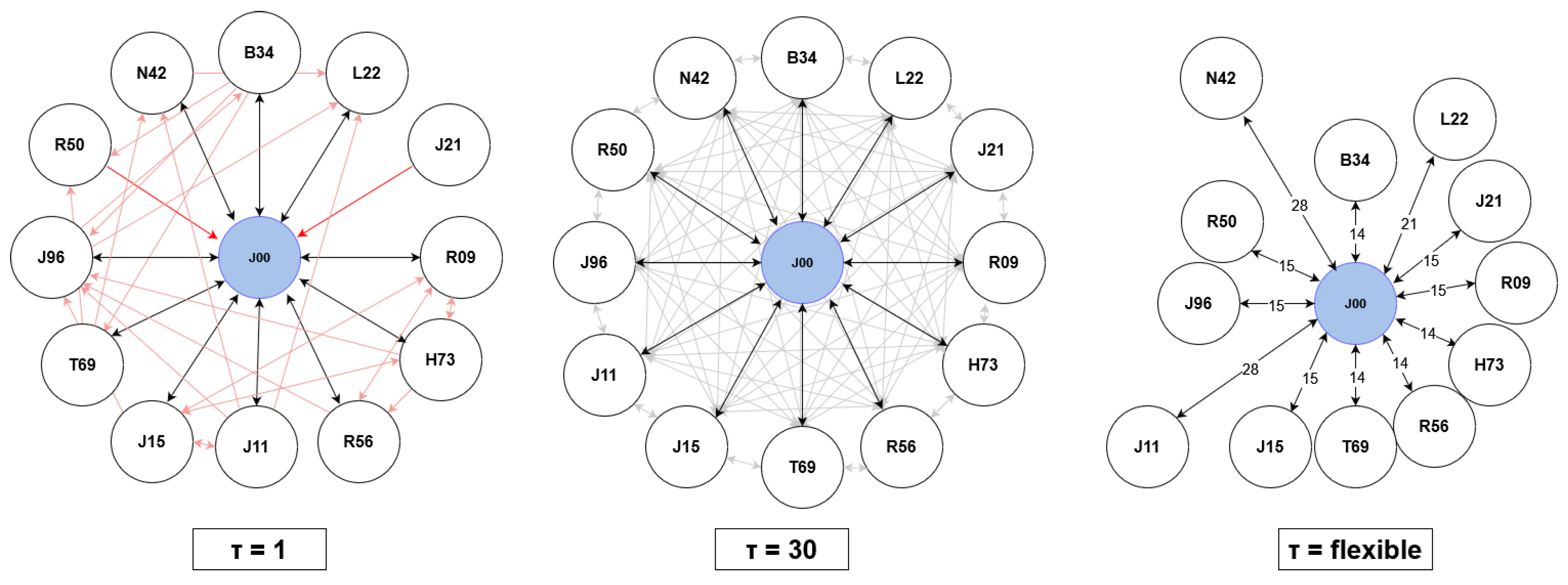
Figure 6, shows the relationship between the variables selected by the GC phase when predicting the target variable. When focusing on the lag value of

θ = 30

(the lag parameter, used to select the predictors), the Granger causal diagram of the variables is fully interconnected. In other words, all variables aid in predicting each other when a 30-day lag is used. Since the objective is to predict the variable J00, the rest of the lines appear blurred. This behavior helps refute the hypothesis that the predictors obtained by the model using a 30-day lag period are correct. For

θ = 1

(1 day lagging time), although all variables G-cause the target variable J00, the method does not output a fully interconnected GC map. The red arrows represent all those relationships that did not meet the assigned p-value and, therefore, do not contribute to predicting the other features. The right image uses a flexible lagging time for each variable selected by the model and the target variable. Although all variables are significantly G-causing the target variable, and the best lagging time according to the AIC method is

θ = 28

, corresponding to 4 weeks and similar to our 30-day lag variable, each variable has an optimal interval correlation time; in other words, the time it takes for the maximum correlation to occur over the entire period. Through these experiments, results obtained with the MLR model are confirmed and also gain knowledge about the system used for prediction and the relationships between variables. This way, the interpretability of the models is enhanced.

When comparing these results with p randomly selected variables in the database, where p is the same number as predictors selected by the lagged MLR model, 40% of the variables do not G-cause the target prediction, while the others may have a GC relation with the target variable, likely due to the seasonality effect. Same behavior is seen with the predictors selected by the Kernel SHAP feature selection procedure. Using p as a threshold to select variables with Kernel SHAP, 40% of them are not GC variables of the target variable.

4.6. Analysis on the Forecasting DL Architectures

Comparing the DL models using the selected subset of predictors refined by the G-causal phase against other predictor subsets allows to assess both the predictive capability of the DL phase and the effectiveness of the feature selection procedure for predictor selection. To perform this evaluation, the predictive performance of the six DL models (GRU, LSTM, BiLSTM, LSTM-ED, CNN-LSTM-ED, VO-CNN-LSTM-ED) is tested using five different subsets of variables as predictors: predictors in the database (1.846, ALL), predictors selected by the lagged MLR phase (12, LAGGED), n predictors refined with the G-causal phase (12, CCLR-DL), n random predictors (12, RANDOM), only the previous values of the target time series as predictors (1, SINGLE) and n predictors selected by the Kernel SHAP feature selection method (12, SHAP).

Table 3 illustrates the MSE numeric results across various architectures and feature selection methods. Consistently, the GRU, LSTM, and BiLSTM architectures outperform others in the majority of experiments. Employing predictors selected by CCLR-DL improves results compared to using either ALL, RANDOM Kernel SHAP post-hoc selection methods across all architectures. Remarkably, across almost all architectures, the most favorable outcomes are achieved whith SINGLE univariate model. These results underscore the detrimental impact of utilizing all variables and high-dimensional datasets, leading to a gradient vanishing problem and yielding inferior results due to numerous uninformative variables, when forecasting a small number of time-steps. Figure 7 depicts the forecasting lines obtained through different feature selection procedures for the BiLSTM architecture under fixed parameters. The illustration demonstrate the accuracy of forecasting obtained by most of the predictor subsets that are able to capture the behaviour of the real time-series. While most experiments yield satisfactory predictions, some exhibit extreme values. CCLR-DL demonstrates superior performance in certain scenarios with different parametrizations.

4.7. Sensitivity Analysis of Look-Back and Forecast Range

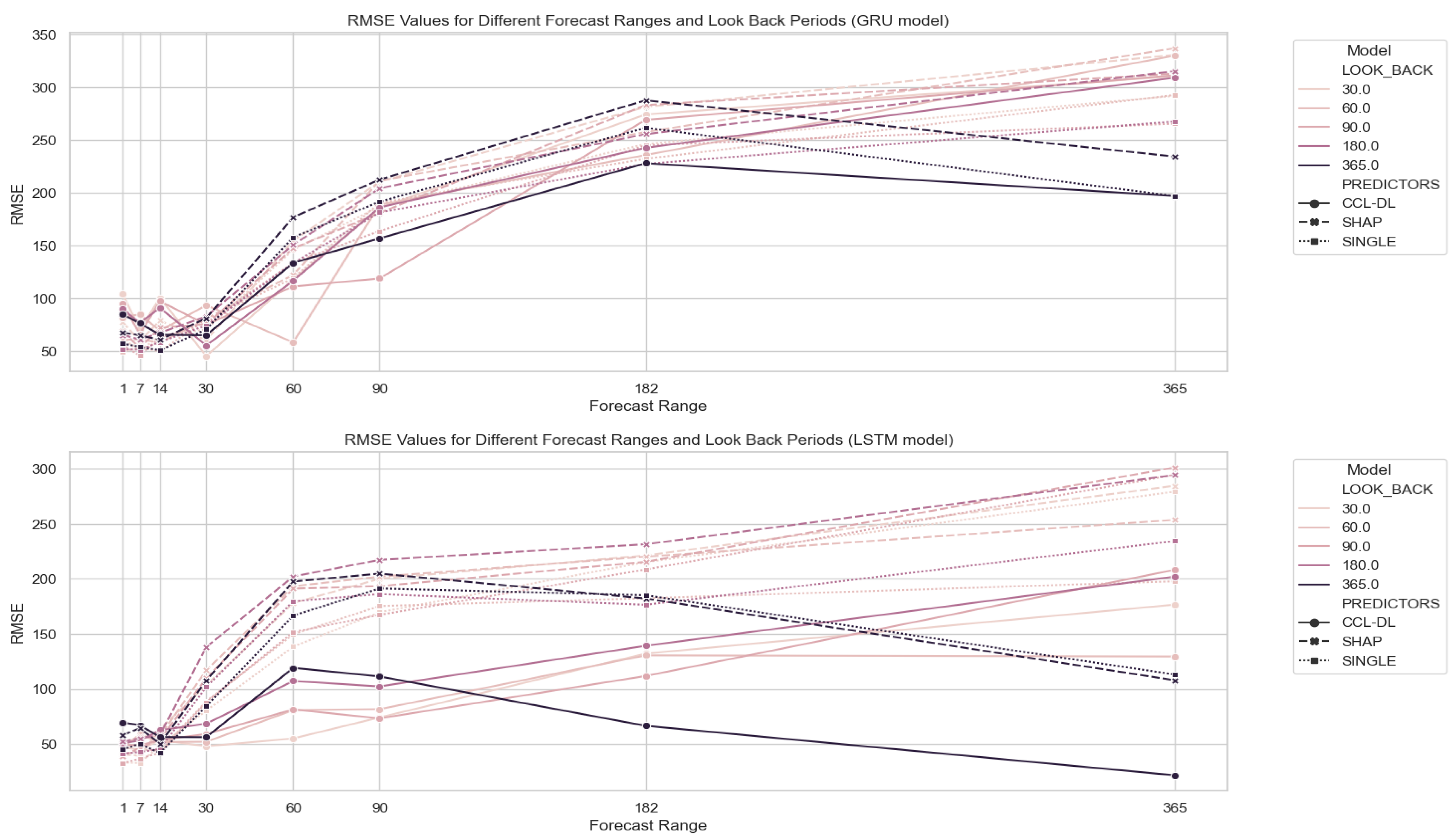
In this section, we focus on the three architectures that yield the best results (GRU, LSTM, and BiLSTM) and the three different variable selection methods that have shown the best results: single predictor, Kernel SHAP feature selection, and CCLR-DL proposal. Subsequently, we assess the prediction performance using different parameterizations of look_back = [30, 60, 90, 182, 365] and forecast_range = [1, 7, 14, 30, 90, 182, 365]. Figure 8 illustrates the results obtained with the feature selection methodology proposed in CCLR-DL.

BiLSTM architecture consistently achieves the best results, followed by GRU, and finally LSTM in the different feature selection scenarios. Figure 9 visualizes the individual results for each of the three architectures, parameters, and feature selection methods.

Regarding the look_back period, contrary to expectations, there is no consistent improvement when using larger look-back times. For all three models, using one year of data proves detrimental. Using 1, 2, 3, or 6 months tend to obtain similar results, with better results obtained by only using the last 30 or 60 days as look-back (consistent with the parameters used for feature selection in the CCLR phases

τ = θ = l o o k_b a c k = 30

Regarding the forecast-range, all three architectures increse the RMSE error as we extend the time horizon, as expected. Nevertheless, except for the case of using a longer look-back value (365 days), in the rest of the look-back periods, there is a point (182 days) where the curve stabilizes and even starts to reduce the error, also with higher forecast ranges.

Particularly interesting is the case of the BiLSTM model (the one achieving better performance), where the CCLR-DL proposal achieves the best results (see Figure 9). For forecast ranges over 7 days, it improves upon the SINGLE proposal. Predicting 14, 30, 60, 90, and 182 days yields better results if it is used for different forecast_range periods. It is noteworthy that the CCLR-DL model achieves the best results in predicting the time series for a 30-day horizon (

τ = 30

), the predefined lag period used in the feature selection phase.

Thus, it can be concluded that the CCLR-DL proposal yields the best results with BiLSTM (the architecture with the lowest RMSE) if the goal is to predict future instances beyond a one-week horizon. For predicting values within a one-week horizon, the three architectures (GRU, LSTM and BiLSTM) produce very similar results, with the best results achieved by the single univariate feature selection dataset.

5. Discussion

In this section, the results of the experimentation are reviewed and discussed. Firstly, an analysis of the feature selection mechanism’s ability to extract knowledge and select the best predictors and its practical implications is conducted (Section 5.1). Second, the forecasting results are analysed and compared with other feature selection strategies (Section 5.2). Finally, the general applicability of the model and its suitability to forecast other variables is discused (Section 5.3).

5.1. Implications of the Results for Feature Selection

The objective of the feature selection phases of CCLR-DL is to select the best subset of variables that aid in predicting a specific target variable without prior knowledge of the relationships among them in a multivariate high dimensional database and also increase model explainability. It consists of two distinct steps: the creation of a lagged MLR model for a predefined lag period to select the predictors, and the use of a GC framework to refine and validate the model, increasing explainability by determining the optimal time period between predictors and the target.

CCLR-DL has been compared to other commonly used methodologies, such as models without explainability notions or other feature selection mechanisms. The former techniques include using the entire database as predictors or transforming the problem into a univariate scenario (using only previous values of the variable for prediction). These models lack explainability because they focus solely on improving the prediction of the variable without considering the context nor the relationship between variables. Despite being faster models (no selection involved), they do not necessarily yield better results. In the case of using all variables as predictors, the algorithms perform poorly because diminish the importance of the target variable as a predictor (gradient vanishing), as many variables in the dataset may not have a direct relationship with the target. On the other hand, using solely past values of the target variable as predictors achieves very good results, as daily values are highly dependent on previous ones. This is due to the seasonal behavior of clinical visits in our database. However, as we move further and aim for more distant predictions, the results deteriorate significantly, and the model lacks other variables that could help to improve them.

The CCLR-DL feature selection method has been also compared to the Kernel SHAP methodology. This does not have a defined method for selecting the optimal number of predictors, unlike CCLR-DL (the reason why the optimal number of variables selected by the are be used in the Kernel SHAP procedure). It’s important to highlight that the Kernel SHAP model obtains Shapley values by fitting a weighted linear regression over predictions obtained for each feature; therefore, the exact computation of Shapley values is computationally challenging. This complexity is exacerbated in our context with a long time series (10 years, 3,650 time steps) and a high number of possible predictors (1,846 variables). Indeed, after training, the variables selected by the model do not seem to have a relationship with the target variable (only 1 out of the 12 is found in the subset of variables selected by CCLR-DL); furthermore, when using the GC phase, we observe that 40% of the selected variables do not have a relationship with the target variable for any determined lag period. The fact that most variables selected by the Kernel SHAP model belong to the first chapter of ICD-10, "Chapter I. Certain infectious and parasitic diseases" leads to believe that the model produces erroneous results and gives more importance to those variables it has encountered first, as the database is sorted in this manner. Unlike CCLR-DL, the Kernel SHAP methodology does not have a lag parameter to help select the best predictors for a given time interval. Although this feature selection method aims to increase both predictive and explanatory capacity, we believe that the results it produces are inaccurate, and the computational time required is excessively high. In contrast to these results, our methodology reduces computational complexity by addressing all collinearities between variables before modeling, eliminating the most correlated ones to simplify the model. This behavior reduces the number of experiments to be tested and, therefore, the overall complexity. Another interesting aspect missing in the case of the Kernel SHAP approach is that CCLR-DL can determine when it has enough variables by evaluating whether the improvement with the addition of a new predictor is significantly better than the SINGLE model. While this behavior is conservative, the algorithm allows some flexibility to assess whether the addition of three unimproving variables could impact the model. Thus, the number of variables to choose does not rely on expertise or pre-selected thresholds.

The GC phase, the second step of the feature selection procedure, serves a dual purpose. On one hand, it is used to refute and refine the subset of predictors selected by the lagged MLR model using the lag value found. On the other hand, once these predictors are refined, a study is conducted for each one to determine the optimal lag value. This step not only allows us to refute the model but also refines it, providing information and explainability. All predictors exhibit an optimal period close to 14, 21, and 28 days, reflecting a weekly periodicity. While a clear explanation for this temporal relationship is lacking, it could be related to the scheduling of physician visits for patients (which might occur weekly). Whether using the subset of variables selected by the Kernel SHAP methodology or randomly selecting an equal number of predictors, none meets the G-causality. 17% of randomly selected variables and 40% of Kernel SHAP variables do not surpass the threshold and therefore do not contribute to the prediction. Our model not only refutes all predictors but also achieves a 100% GC relationship between all variables in the model: all variables, both target and predictors, are significantly correlated with each other in the G-causal matrix for the computed lag.

When focusing on the predictors selected by CCLR-DL, most have been related or are easily associable as causes, symptoms, or consequences of the target variable, "J00: Acute nasopharyngitis [common cold]" Some of these predictors (defined in Table 4), such as "L22: Diaper dermatitis", "H73: Other disorders of tympanic membrane" or "T69: Other effects of reduced temperature" could refer to variables describing a population cohort. These variables are often linked to consultations for the pediatric population, a cohort that can be easily related to diagnoses of the common cold. On the other hand, variables like "J11: Influenza, virus not identified", "J15: Bacterial pneumonia, not elsewhere classified", "J21: Acute bronchiolitis" and "J96: Respiratory failure, not elsewhere classified" may refer to potential causes of nasopharyngitis, such as viral or bacterial infections, from the same chapter as the target variable. Finally, variables like "R09: Other symptoms and signs involving the circulatory and respiratory systems", "R50: Fever of other and unknown origin" and "R56: Convulsions, not elsewhere classified" might refer to symptoms or consequences of the disease. All these relationships should be further validated in subsequent studies. The predictors selected with the Kernel SHAP methodology have a more diffuse relationship. Only one of the predictors is found in both subsets ("B34: Viral infection of unspecified site"). The rest of the predictors are: J02, A01, A08, A07, A23, A02, A22, A15, A17, A20, A05. This overrepresentation of variables from the chapter "Chapter I. Certain infectious and parasitic diseases" could indicate a malfunction of the method.

Table 4. Predictors selection by CCLR-DL framework for the higher incidence ICD-10 code J00.

Lag	Code	Description
14	B34	Viral infection of unspecified site.
21	L22	Diaper [napkin] dermatitis.
14	H73	Other disorders of tympanic membrane.
14	T69	Other effects of reduced temperature.
15	J11	Influenza, virus not identified.
15	J15	Bacterial pneumonia, not elsewhere classified.
28	J21	Acute bronchiolitis.
15	J96	Respiratory failure, not elsewhere classified.
15	R09	Other symptoms and signs involving the circulatory and respiratory systems.
14	R50	Fever of other and unknown origin.
15	R56	Convulsions, not elsewhere classified.

5.2. Implications of Forecasting Results

The forecasting phase aims to determine the best Deep Learning architecture for predicting clinical demand associated with diagnostics. The various architectures have parameterizations that have been optimized using a grid search. Different algorithms have been evaluated based on the parameters: length of observation periods for prediction (look-back) and number of time steps to predict (forecast range). To achieve this, the results of different architectures are compared in terms of forecasting accuracy and, at the same time, validate the feature selection strategy by comparing it with other selection methods. Different architectures have been evaluated using all diagnoses (1,846), an univariate single model, our model, random variable selection (same number of variables as CCLR-DL to avoid dimension effect), and Kernel SHAP for specific parameterizations.

Within a one-week horizon, best results are obtained by using an univariate single model that relies solely on the target variable as a demand predictor. These results demonstrate that clinical visits have a very strong seasonal component with correlated close values. In this context, the application of a feature selection method can be counterproductive as it increases noise and diminishes the importance of the target sequence as a predictor. Conversely, a one-week horizon may prove insufficient for demand prediction, emphasizing the importance of extending forecast periods whenever feasible. Typically, as the forecast range expands, errors tend to stabilize or decrease, as depicted in Figure A1. In such scenarios, with extended forecast ranges, the CCLR-DL methodology surpasses univariate single models, as future values are likely to be influenced more by external factors and less by previous values of the target time series.

The average improvement of a single model versus our proposal, measured by RMSE, is 19.8%. CCLR-DL is 60.1% better than not using any feature selection technique and 51.9% than randomly selecting predictors. When the goal of the experimentation is to forecast a number of time steps beyond 7 days and up to 182 (including the 30 used in the predefined lag parameter) CCLR-DL achieves better results than all other approaches. Results suggest that for predicting near-future values, the target sequence plays an important role; but this could be of low relevance for health resources management. However, as we extend the forecasting horizon, the algorithm can add features that significantly improve results, incorporating nonlinear information that has a positive impact on accuracy. Since CCLR-DL obtains the best results when predicting a number of time steps equal to the predefined lag demonstrates the suitability of the approach as a hybrid forecasting method that uses only one parameter to select and predict time-series data.

Increasing the number of time steps fitted for prediction does not result in improvement for any of the architectures or feature subsets used, contrary to what might be expected. If the goal is to predict less than a week’s timesteps all experiments yield similar results. When predicting longer time periods, using 30, 60, 90, or 180 timesteps produces analogous results, while using 365 leads to worse outcomes. Regarding the forecast_range parameter, as seeking to predict more time steps, the error gradually increases, as expected. It is interesting to note that the error stabilizes and even decreases when attempting to predict 365-time steps for look_back times less than 365.

If focusing on the comparison of architectures used, in most experiments, the best results are obtained by simpler RNN methodologies like GRU, LSTM, and BiLSTM. In the experiments to refine the parameters of the forecasting layer, only the three best architectures and feature selection methods have been used. The methodology with better results for each experiment highly depends on the subset of variables used. For those subsets with better results (single, Kernel SHAP, and our methodology) BiLSTM obtains the best results. These are likely since this architecture performs well in detecting non-linear trends in time series, beyond the linear behavior inherent in the variables. The use of two RNNs to capture the forward and backward signals improves the results compared to other architectures. In the future, it could be interesting to explore others based on BiLSTM that have shown promising performance, such as the BiLSTM-CNN[49]. Another interesting experiment would be to over-represent the target sequence in the prediction set when predicting a few time steps, a moment when more importance should be given to the values of the target time series as predictors.

5.3. General Aplicability of the Model

The methodology proposed in this study aims to improve the prediction of variables in large temporal databases without prior knowledge of the underlying relationship between them. The method allows the enhancement of variable prediction while increasing the interpretability of the model through the selection of a subset of features that improve prediction for a time lag. This is made possible through a hybrid model that uses conventional statistical models such as multivariate regression and GC to select predictors and benefits from new DL-based prediction architectures to improve forecasting. To verify the effectiveness of the model, the study focused on hospital demand for visits linked to diagnoses, taking the diagnosis "J00: Acute nasopharyngitis [common cold]" (the code with the most visits during the study period from 2010 to 2020) as the study objective. These results are not only found in the case of the J00 diagnosis but are also repeated in the two other most coded diagnoses in the database.

The results presented in this article demonstrate that for a predefined forecasting period exceeding 7 days, our methodology is effective in selecting a subset of predictor variables that GC the target variable, improving accuracy in forecasting using a BiLSTM-based RNN architecture. For predictions within a one-week horizon, it is more effective to use only previous values of the target time series as predictors. The features selected by the model have a clear relationship with the diagnosis, as they belong to the same chapter of the International Classification of Diseases (ICD) or could be causes, symptoms, or related effects such as viral infections or symptoms previously associated with the patient cohort. The fact that not all the experimented target variables are epidemiological (e.g., "M54: Dorsalgia," "T14: Injury of unspecified body region") demonstrates that the way the population interacts with the healthcare system for specific reasons follows seasonal patterns and can be predicted, even if they are not population transmitted diseases. This behavior suggests that a minimum number of visits related to the diagnosis is required for prediction. Therefore, for less frequent diagnoses, not explored in this work, it is more challenging to identify correlations or find dependencies between past and future values. During holidays, specific months of the year, as well as days of the week, the population follows interaction patterns with the Catalan healthcare system. This indicates that utilizing these variables, which have a clear impact on time series, such as the month of the year, holidays, or days of the week, would help improve predictions and achieve lower accuracy. Obtaining accurate forecastings of clinical demand can represent a significant improvement for public healthcare systems, as it could help redistribute specialized resources based on healthcare demand and prepare for disruptions in the system in severe cases such as COVID-19, thus contributing to resource savings; the proposed methodology is capable of predicting real-time series in high-dimensional databases, in this case, clinical demand, using a time lag. Since different models can be obtained with different time lags, healthcare managers could take advantage and use the model that best fits their needs. Moreover, this methodology not only identifies predictors and achieves good forecasting results, surpassing other proposals but also enhances the understanding of the database context and interpretability by determining the optimal time interval for correlation between predictors and the target variable. CCLR-DL is easily adaptable to any high-dimensional temporal database without prior knowledge of the database context.

6. Conclusions

This paper proposes CCLR-DL, a novel hybrid methodology that integrates a lagged MLR model and Granger causality for predictor selection alongside RNN models to forecast multivariate high-dimensional time-series datasets without prior knowledge of variables importance and relations. By using a lagged MLR and Granger causality, CCLR-DL selects and refines the best set of predictors for a target time series with a predefined lag. This not only improves forecasting in the deep learning (DL) phase but also enhances explainability by identifying the optimal time difference between predictors and the target variable. The lagged MLR phase is useful for revealing the linear part of the time series, while the DL step allows modeling the nonlinear behavior; according to the experimental results, single-variable models perform better for up to a week predictions, but CCLR-DL achieves superior results than models using a single variable, all variables, or a standard feature selection method such as SHAP for predicting values beyond a week, offering superior performance and interpretability without additional parameters beyond the forecasting horizon, thereby reducing the expertise required by the user. Forecasting demand beyond a week seems a more promising supportive outcome for healthcare managers. Among all implemented DL architectures, BiLSTM emerges as the best-proposed model, followed by simple RNN models such as GRU and LSTM. The experiments conducted in this article utilize real-world data from the public Catalan healthcare system and demonstrate that clinical visit demand associated with diagnostics can be forecasted with considerable accuracy, even if these are not epidemiological, opening up promising avenues for further investigation.

Future research should focus on exploring the algorithm’s potential to forecast less common diagnoses characterized by more erratic behaviors, presenting greater forecasting challenges. Regarding the current approach, the MLR model is defined using a lag value of 30, yet during the forecasting phase, various forecast ranges beyond 30 are evaluated. Remarkably, the CCLR-DL model outperforms others in predicting outcomes from 30 days ahead. These findings demonstrate the model’s efficacy. Further research is necessary to explore the methodology’s complete potential. Additionally, analyzing different lag values based on Granger causality analysis presents an intriguing avenue for research, challenging machine learning methods to effectively handle time series of varying lengths simultaneously.

Acknowledgments

Computational resources were partially provided by the Agency for Health Quality and Assessment of Catalonia (AQuAS), in particular by the team of the Program of Data Analysis for Health Research and Innovation (PADRIS).

Appendix A. Notation

M	Time series dataset
D	Set of diagnoses
$d_{i} \in D$	Single diagnosis
$d_{g} \in D$	Target diagnosis
N	Number of diagnoses (= $\| D \|$ )
T	Set time stamps
$t_{i} \in T$	Time point
L	Number of time points (= $\| T \|$ )

$Δ$	Selected diagnoses from collinearity analysis
$δ_{i} \in Δ$	Selected diagnosis in $Δ$
P	Selected diagnoses from Lagged MLR (predictors)
p	Number of predictors in the lagged model (= $\| P \|$ )
A	Selected diagnoses from GC (GC predictors)

$τ$	Slag variable for Lagged MLR (feature selection)
$θ$	Causality lag
$θ_{i, g}$	Best lag for predictor $d_{j}$ regarding $d_{g}$

k	Look back for forecasting
f	Forecast range
$X_{p, k}$	Batch input for DL
$Y_{f}$	Forecasting of DL

Appendix B. Results Other Diagnoses

This appendix section aims to demonstrate the results of the algorithm with other diagnoses that have a significant incidence in the population. Specifically, the diagnoses used are "M54: Dorsalgia" and "T14: Injury of the unspecified body region." These diagnoses, along with the diagnosis "J00," represent the top three diagnoses with the highest incidence in Primary Care from 2010 to 2020. It is important to note that these diagnoses do not have an epidemiological nature, and therefore, their prediction would be more related to the population’s behavior with the healthcare system and other predictors than to the effect of the time series itself in forecasting.

Tables below describe the selected predictors for each diagnosis and the results of the best architecture of the DL layer, along with a comparison with other predictor subsets and forecast and lookback ranges.

Table A1. Predictors selection by CCLR-DL framework for the 2 higher incidence ICD-10 codes).

Lag	Code	Description
-	M54	Sciatica
14	A60	Anogenital herpesviral [herpes simplex] infection
14	S43	Dislocation, sprain and strain of joints and ligaments of shoulder girdle
21	K59	Other functional intestinal disorders
14	G50	Disorders of trigeminal nerve
14	S82	Fracture of lower leg, including ankle
14	N12	Tubulo-interstitial nephritis, not specified as acute or chronic
14	I63	Cerebral infarction
21	R31	Unspecified haematuria
21	I26	Pulmonary embolism
21	K29	Gastritis and duodenitis
21	Z33	Pregnant state, incidential
21	K20	Oesophagitis
-	T14	Injury of unspecified body region
35	Y04	Assault by bodily force
38	R33	Retention of urine
35	L90	Atrophic disorders of skin
35	H15	Disorders of sclera
38	K12	Stomatitis and related lesions
35	N17	Acute renal failure
35	P38	Omphalitis of newborn with or without mild haemorrhage
38	Q67	Congenital musculoskeletal deformities of head, face, spine and chest

Figure A1. Best DL architecture forecasting results for the 2 higher incidence ICD-10 codes (other than J00). (Top) CCLR-DL obtains best results for M54 code and GRU architecture. (Bottom) CCLR-DL obtains best results for T14 code and LSTM architecture.

References

Pérez Sust, P.; Solans, O.; Fajardo, J.; Medina Peralta, M.; Rodenas, P.; Gabaldà, J.; Garcia Eroles, L.; Comella, A.; Velasco Muñoz, C.; Sallent Ribes, J.; Roma Monfa, R.; Piera-Jimenez, J. Turning the Crisis Into an Opportunity: Digital Health Strategies Deployed During the COVID-19 Outbreak. JMIR Public Health Surveillance 2020, 6, e19106. [Google Scholar] [CrossRef] [PubMed]
Arolas, H.P.; Vidal-Alaball, J.; Gil, J.; Seguí, F.L.; Nicodemo, C.; Saez, M. Missing Diagnoses during the COVID-19 Pandemic: A Year in Review. International J. of Environmental Research and Public Health 2021, 18, 5335. [Google Scholar] [CrossRef] [PubMed]
Perramon-Malavez, A.; Bravo, M.; de Rioja, V.L.; Català, M.; Alonso, S.; Álvarez Lacalle, E.; López, D.; Soriano-Arandes, A.; Prats, C. A semi-empirical risk panel to monitor epidemics: Multi-faceted tool to assist healthcare and public health professionals. Frontiers in Public Health 2024, 11, 1307425. [Google Scholar] [CrossRef] [PubMed]
López Seguí, F.; Hernández Guillamet, G.; Pifarré Arolas, H.; Marin-Gomez, F.X.; Ruiz Comellas, A.; Ramirez Morros, A.M.; Adroher Mas, C.; Vidal-Alaball, J. Characterization and Identification of Variations in Types of Primary Care Visits Before and During the COVID-19 Pandemic in Catalonia: Big Data Analysis Study. J Med Internet Res 2021, 23, e29622. [Google Scholar] [CrossRef] [PubMed]
Garcia-Olive, I.; López Seguí, F.; Hernández Guillamet, G.; Vidal-Alaball, J.; Abad, J.; Rosell, A. Impact of the COVID-19 pandemic on diagnosis of respiratory diseases in the Northern Metropolitan Area in Barcelona (Spain). Medicina Clínica 2023, 160, 392–396. [Google Scholar] [CrossRef] [PubMed]
Barker, J. Machine learning in M4: What makes a good unstructured model? International Journal of Forecasting 2020, 36, 150–155. [Google Scholar] [CrossRef]
Casolaro, A.; Capone, V.; Iannuzzo, G.; Camastra, F. Deep Learning for Time Series Forecasting: Advances and Open Problems. Information 2023, 14. [Google Scholar] [CrossRef]
Bharati, S.; Mondal, M.R.H.; Podder, P. A Review on Explainable Artificial Intelligence for Healthcare: Why, How, and When? IEEE Transactions on Artificial Intelligence 2023, 1–15. [Google Scholar] [CrossRef]
Lundberg, S.M.; Lee, S.I. A Unified Approach to Interpreting Model Predictions. In Proceedings of the 31st International Conference on Neural Information Processing Systems; 2017; pp. 4768–4777. [Google Scholar]
Spiliotis, E. Time Series Forecasting with Statistical, Machine Learning, and Deep Learning Methods: Past, Present, and Future; 2023; pp. 49–75. [CrossRef]
Spencer, R.J.; Amer, S.; George, E.J.S. A retrospective analysis of emergency referrals and admissions to a regional neurosurgical centre 2016–2018. British J. of Neurosurgery 2021, 35, 438–443. [Google Scholar] [CrossRef]
Wang, W.W.; Li, H.; Cui, L.; Hong, X.; Yan, Z. Predicting Clinical Visits Using Recurrent Neural Networks and Demographic Information. Proceedings of the 2018 IEEE 22nd International Conference on Computer Supported Cooperative Work in Design, CSCWD 2018 2018, 785–789. [Google Scholar] [CrossRef]
Arielle, S.; Drake, A.; Emily, G.L., W.T.; Benson, H.; Cheryl, W. Predicting unplanned medical visits among patients with diabetes: translation from machine learning to clinical implementation. BMC Med. Inform. Decis. Mak. 2021, 31, 111. [Google Scholar] [CrossRef]
Upadhyay, R.K.; Kumari, N.; Rao, V.S.H. Modeling the spread of bird flu and predicting outbreak diversity. Nonlinear Analysis: Real World Applications 2008, 9, 1638–1648. [Google Scholar] [CrossRef] [PubMed]
Kırbaş, I.; Sözen, A.; Tuncer, A.D.; Şinasi Kazancıoğlu, F. Comparative analysis and forecasting of COVID-19 cases in various European countries with ARIMA, NARNN and LSTM approaches. Chaos, Solitons, and Fractals 2020, 138, 110015. [Google Scholar] [CrossRef] [PubMed]
Ibrahim, M.; Jemei, S.; Wimmer, G.; Hissel, D. Nonlinear autoregressive neural network in an energy management strategy for battery/ultra-capacitor hybrid electrical vehicles. Electric Power Systems Research 2016, 136, 262–269. [Google Scholar] [CrossRef]
Chandra, R.; Jain, A.; Chauhan, D.S. Deep learning via LSTM models for COVID-19 infection forecasting in India. PLoS ONE 2021, 17, e0262708. [Google Scholar] [CrossRef] [PubMed]
Chimmula, V.K.R.; Zhang, L. Time series forecasting of COVID-19 transmission in Canada using LSTM networks. Chaos, Solitons & Fractals 2020, 135, 109864. [Google Scholar] [CrossRef]
Shahid, F.; Zameer, A.; Muneeb, M. Predictions for COVID-19 with deep learning models of LSTM, GRU and Bi-LSTM. Chaos, Solitons & Fractals 2020, 140, 110212. [Google Scholar] [CrossRef]
Sil, A.; Kumar, V.N. Does weather affect the growth rate of COVID-19, a study to comprehend transmission dynamics on human health. Journal of Safety Science and Resilience 2020, 1, 3–11. [Google Scholar] [CrossRef]
Sarkodie, S.A.; Owusu, P.A. Impact of meteorological factors on COVID-19 pandemic: Evidence from top 20 countries with confirmed cases. Environmental Research 2020, 191, 110101. [Google Scholar] [CrossRef]
Ahlawat, A.; Wiedensohler, A.; Mishra, S.K. An Overview on the Role of Relative Humidity in Airborne Transmission of SARS-CoV-2 in Indoor Environments. Aerosol and Air Quality Research 2020, 20, 1856–1861. [Google Scholar] [CrossRef]
Towfiqul, I.A.R.; M, H.; Azad, A.A.K.; Roquia, S.; Zannat, T.F.; Islam, K.S.; Moniru, A.G.M.; M. , I.S. Effect of meteorological factors on COVID-19 cases in Bangladesh. Environment, Development and Sustainability 2021, 23, 9139–9162. [Google Scholar] [CrossRef]
López, B.; Torrent-Fontbona, F.; Roman, J.; Inoriza, J.M. Forecasting of emergency department attendances in a tourist region with an operational time horizon 2021.
Mathonsi, T.; van Zyl, T. A Statistics and Deep Learning Hybrid Method for Multivariate Time Series Forecasting and Mortality Modeling. Forecasting 2022, 4, 1–25. [Google Scholar] [CrossRef]
Harvey, A.C. Analysis and Generalisation of a Multivariate Exponential Smoothing Model. Management Science 1986, 32, 374–380. [Google Scholar] [CrossRef]
Pfeffermann, D.; Allon, J. Multivariate exponential smoothing: Method and practice. International J. of Forecasting 1989, 5, 83–98. [Google Scholar] [CrossRef]
Xu, W.; Peng, H.; Zeng, X.; Zhou, F.; Tian, X.; Peng, X. A hybrid modelling method for time series forecasting based on a linear regression model and deep learning. Applied Intelligence 2019, 49, 3002–3015. [Google Scholar] [CrossRef]
Granger, C.W.J. Investigating Causal Relations by Econometric Models and Cross-spectral Methods. Econometrica 1969, 37, 424. [Google Scholar] [CrossRef]
Kim, M. Time-series dimensionality reduction via Granger causality. IEEE Signal Processing Letters 2012, 19, 611–614. [Google Scholar] [CrossRef]
Yang, D.; Chen, H.; Song, Y.; Gong, Z. Granger Causality for Multivariate Time Series Classification. 2017, pp. 103–110. [CrossRef]
Chen, Y.; Rangarajan, G.; Feng, J.; Ding, M. Analyzing multiple nonlinear time series with extended Granger causality. Physics Letters, Section A: General, Atomic and Solid State Physics 2004, 324, 26–35. [Google Scholar] [CrossRef]
Sun, X. Assessing Nonlinear Granger Causality from Multivariate Time Series. Machine Learning and Knowledge Discovery in Databases 2008, 440–455. [Google Scholar]
Freedman, D.; Pisani, R.; Purves, R. Statistics: Fourth International Student Edition; 2007.
Johnston, R.; Jones, K.; Manley, D. Confounding and collinearity in regression analysis - a cautionary tale and an alternative procedure, illustrated by studies of British voting behaviour. Quality and Quantity 2018, 52, 1957–1976. [Google Scholar] [CrossRef]
Frank, J.; Massey, J. The Kolmogorov-Smirnov Test for Goodness of Fit. Journal of the American Statistical Association 1951, 46, 68–78. [Google Scholar] [CrossRef]
White, H. A Heteroskedasticity-Consistent Covariance Matrix Estimator and a Direct Test for Heteroskedasticity. Econometrica 1980, 48, 817–838. [Google Scholar] [CrossRef]
Kwiatkowski, D.; Phillips, P.C.; Schmidt, P.; Shin, Y. Testing the null hypothesis of stationarity against the alternative of a unit root: How sure are we that economic time series have a unit root? Journal of Econometrics 1992, 54, 159–178. [Google Scholar] [CrossRef]
Fuller, W. Introduction to Statistical Time Series; 1995.
Walker, G.T. On Periodicity in Series of Related Terms. Proceedings of The Royal Society A: Mathematical, Physical and Engineering Sciences 1931, 131, 518–532. [Google Scholar] [CrossRef]
Akaike, H. A New Look at the Statistical Model Identification. IEEE Transactions on Automatic Control 1974, 19, 716–723. [Google Scholar] [CrossRef]
Schwarz, G. Estimating the Dimension of a Model. Ann. Statist. 1978, 6, 461–464. [Google Scholar] [CrossRef]
Hochreiter, S.; Schmidhuber, J. Long Short-Term Memory. Neural Computation 1997, 9, 1735–1780. [Google Scholar] [CrossRef]
Chung, J.; Gulcehre, C.; Cho, K.; Bengio, Y. Empirical Evaluation of Gated Recurrent Neural Networks on Sequence Modeling. NIPS 2014 Workshop on Deep Learning, 2014.
Graves, A.; Schmidhuber, J. Framewise phoneme classification with bidirectional LSTM and other neural network architectures. Neural Networks 2005, 18, 602–610. [Google Scholar] [CrossRef]
Cho, K.; van Merriënboer, B.; Gulcehre, C.; Bahdanau, D.; Bougares, F.; Schwenk, H.; Bengio, Y. Learning Phrase Representations using RNN Encoder–Decoder for Statistical Machine Translation. In Proceedings of the 2014 Conference on Empirical Methods in Natural Language Processing (EMNLP); 2014; pp. 1724–1734. [Google Scholar] [CrossRef]
Ang Zhang and Xiaoyong Zhao and Lei Wang. IEEE Information Technology, Networking, Electronic and Automation Control Conference, ITNEC 2021, Oct, pp. 571-575. CNN and LSTM based Encoder-Decoder for Anomaly Detection in Multivariate Time Series, 2021. [CrossRef]
Organization, W.H. ICD-10 : International statistical classification of diseases and related health problems : Tenth revision, 2004.
Staffini, A. A CNN-BiLSTM Architecture for Macroeconomic Time Series Forecasting. Engineering Proceedings 2023, 39. [Google Scholar] [CrossRef]

1	Perform preprocessing such as successive differentiation to reduce or eliminate non-stationarity.

Figure 1. Comprehensive Cross-Correlation and Lagged Linear Regression Deep Learning (CCLR-DL) framework.

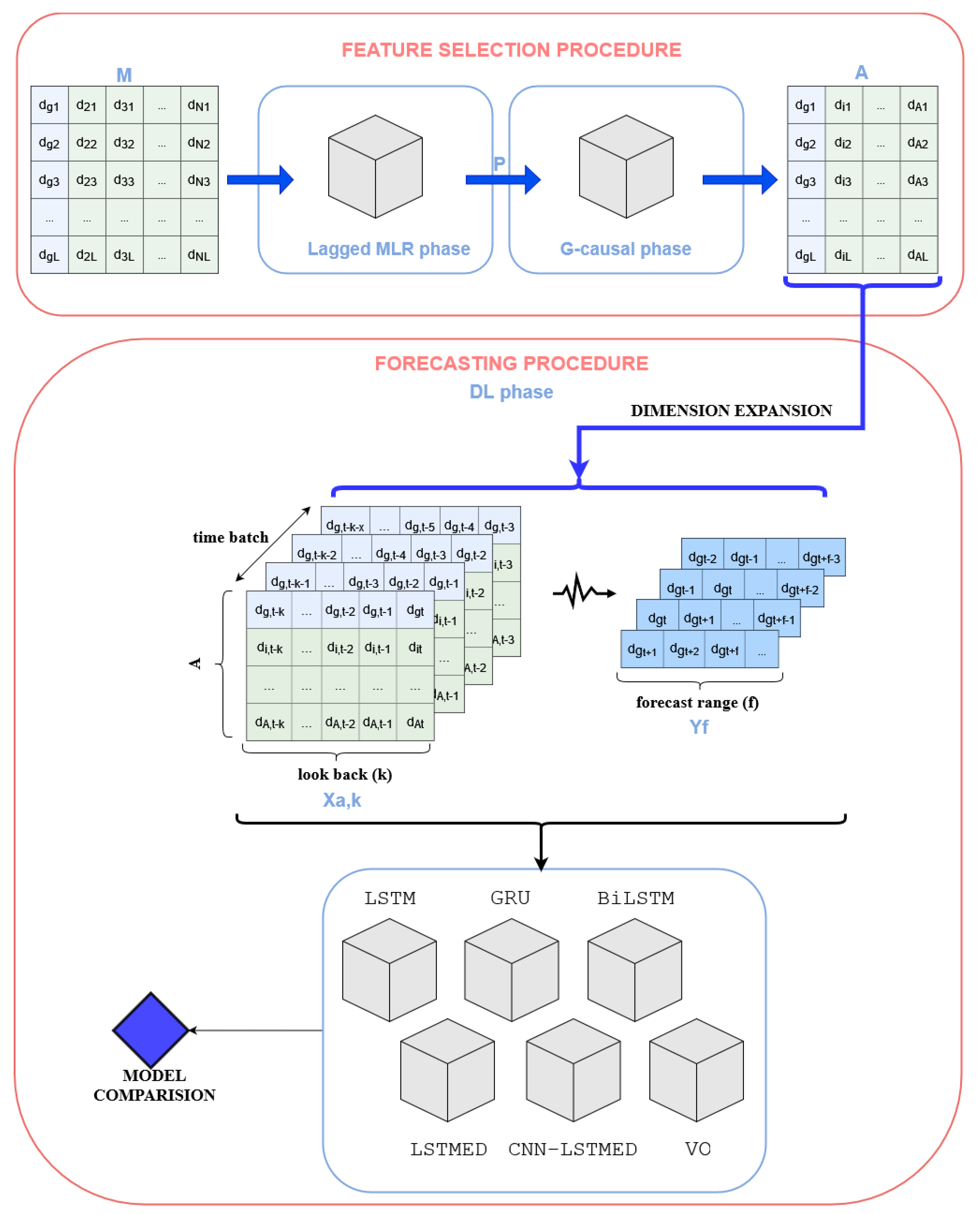
Figure 2. Lagging multiple linear regression phase model construction.

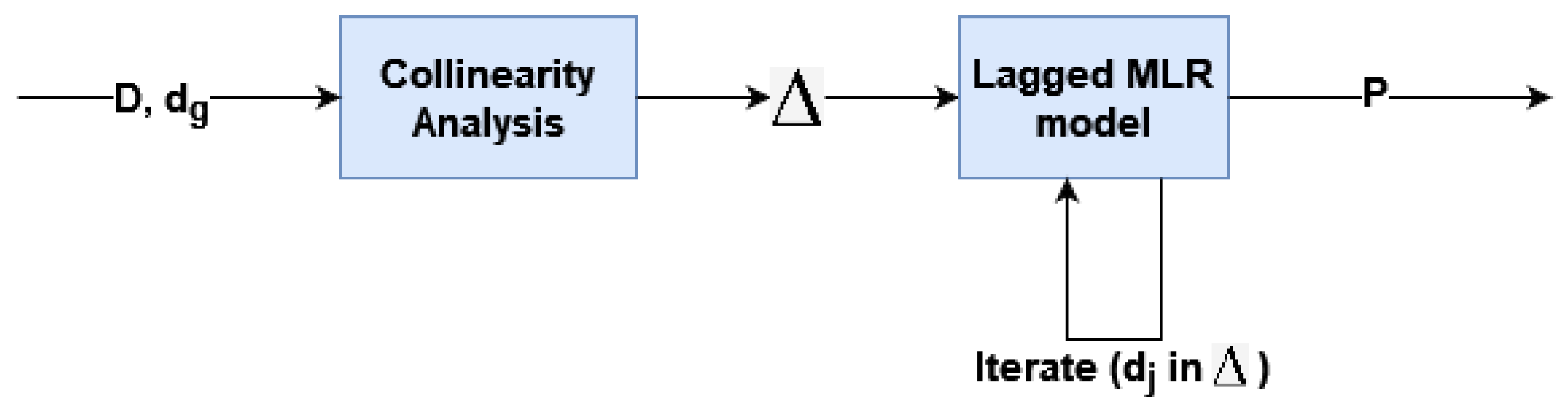
Figure 3. top 10 daily diagnoses with higher demand.

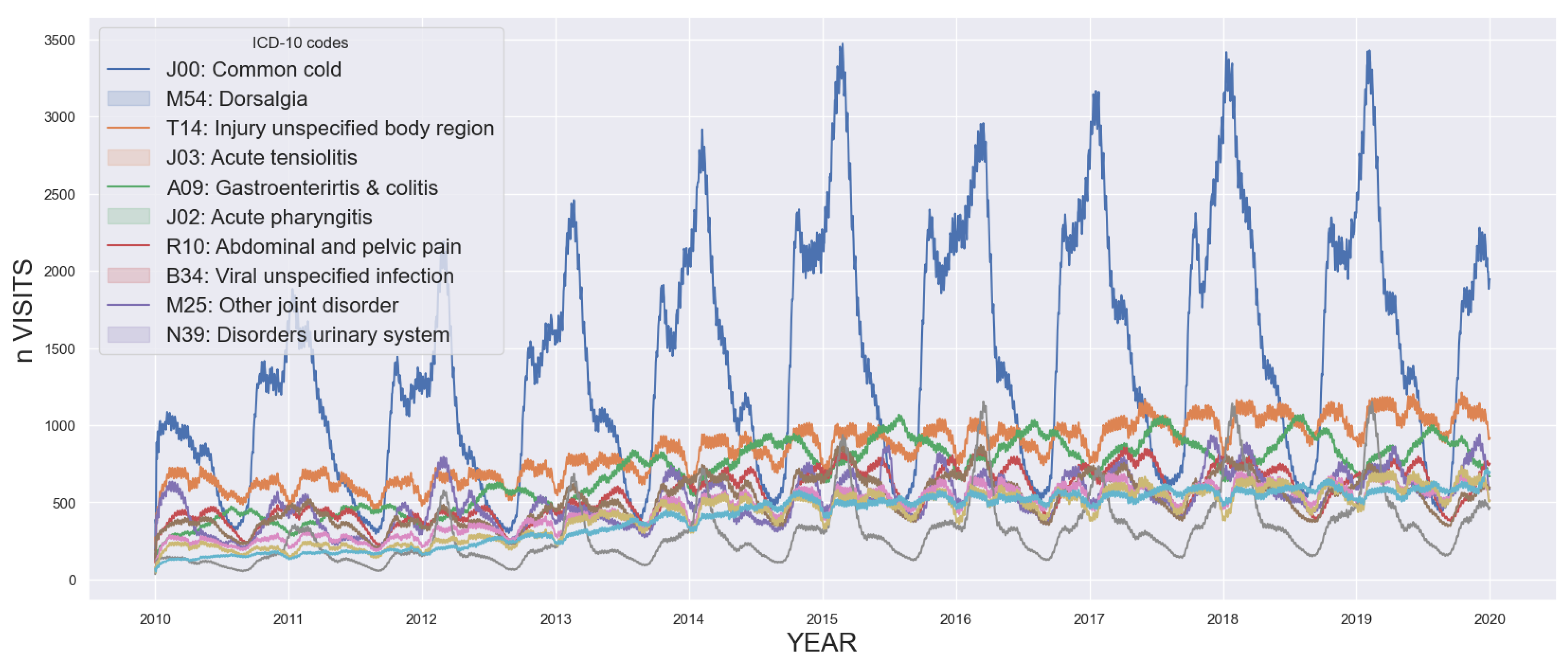
Figure 4. MAPE for the best models depending on lag

τ

in [0,30].

Figure 4. MAPE for the best models depending on lag

τ

in [0,30].

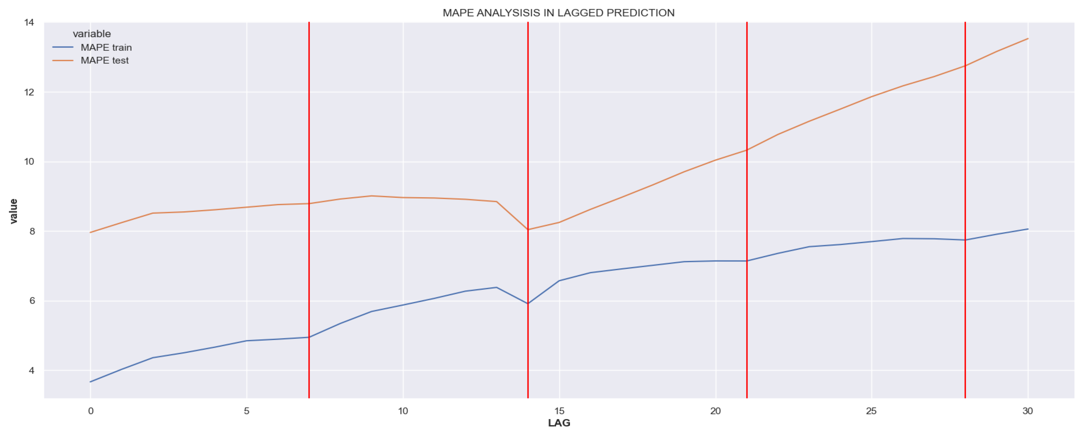
Figure 5. Performance of lagged MLR when considering the predictors selected in iteration 13 (blue), 21 (red) and 26 (green). Real

d_{g} = J 00

time series is shown in a doted, green line. Y axis is normalized and scaled for regression improvement.

Figure 5. Performance of lagged MLR when considering the predictors selected in iteration 13 (blue), 21 (red) and 26 (green). Real

d_{g} = J 00

time series is shown in a doted, green line. Y axis is normalized and scaled for regression improvement.

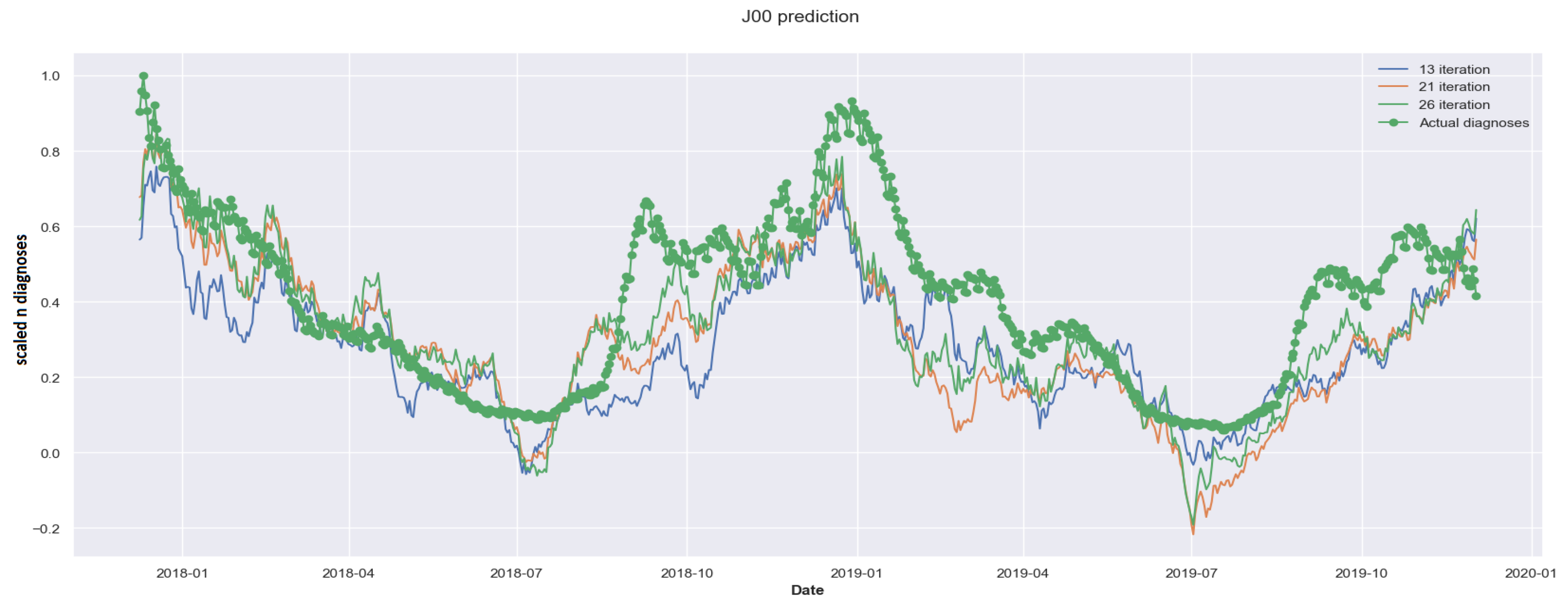
Figure 7. Effect of different feature selection methods in forecasting accuracy using the BiLSTM model. (look_back=30 and forecast_range = 7)

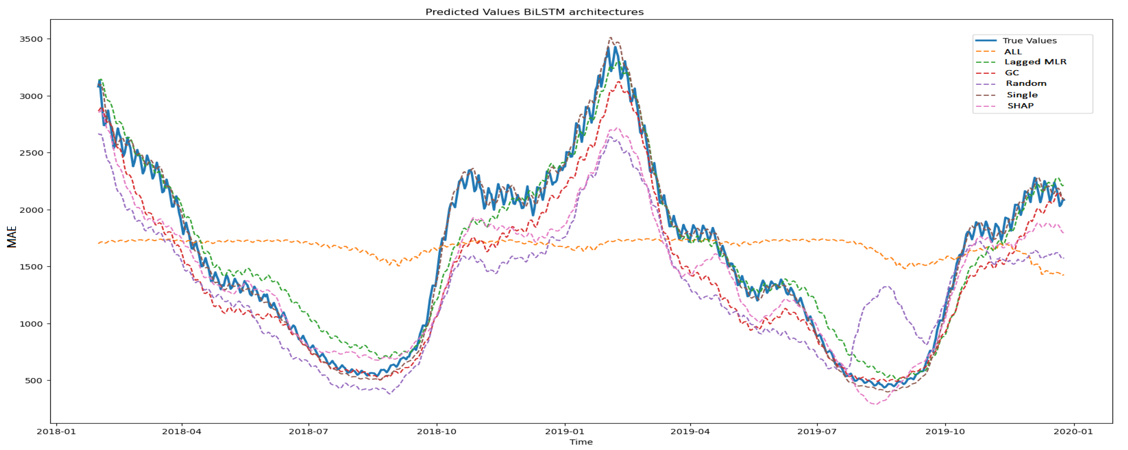
Figure 8. RMSE values with CCLR-DL predictor selection procedure.

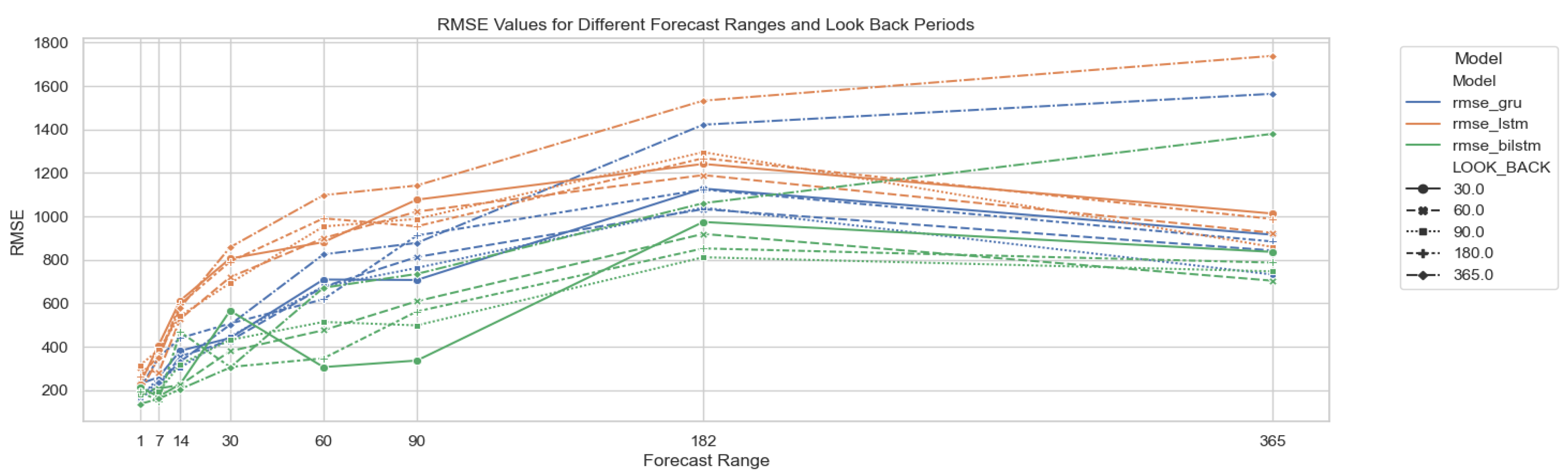
Figure 9. RMSE results for three DL architectures: GRU, LSTM and BiLSTM. Results for different parametrizations of look_back and forecast_range periods. Different line shapes correspond to the three feature methods yielding better results in forecasting: CCLR-DL, Kernel SHAP and single univariate model.

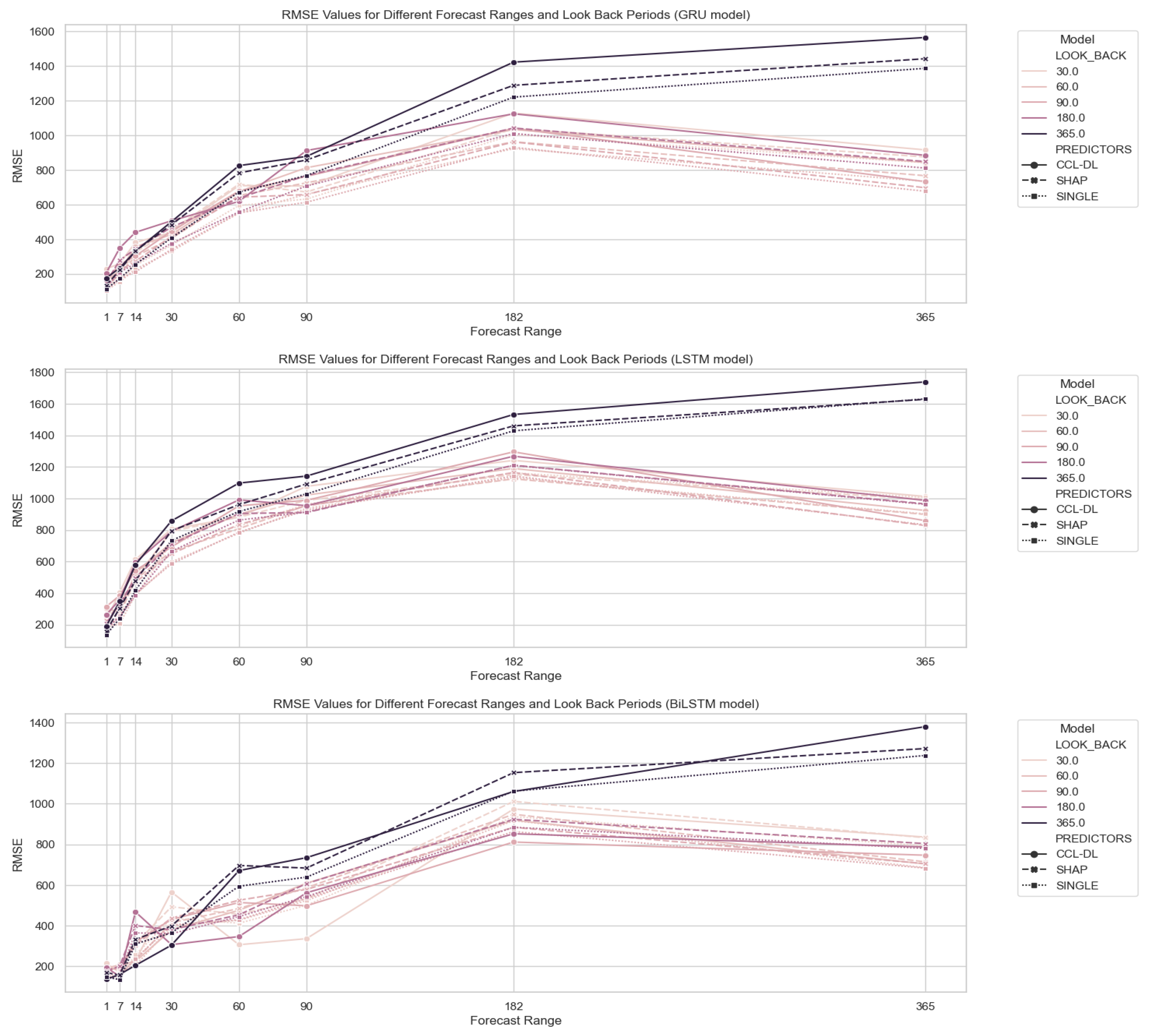
Table 1. Parametritzations used in each architecture.

Algorithm	Epochs	Batch_size	Optimizer
LSTM	30	80	Nadam
GRU	100	80	Adam
BiLSTM	100	500	Adam
LSTM-ED	200	10	Adamax
CNN-LSTM-ED	20	500	Nadam
VO-CNN-LSTM-ED	50	10	Adam

Table 2. Lagging MLR model performance according to different lags (

τ

Table 2. Lagging MLR model performance according to different lags (

τ

lag ( $τ$ )	p-val (F1)	p-val (F2)	RMSE (train)	RMSE (test)	p
0	0.627	1.000	0.051	0.097	12
1	0.692	1.000	0.056	0.102	12
7	0.107	0.000	0.071	0.108	12
14	0.215	0.001	0.081	0.105	22
30	0.267	1.000	0.112	0.175	12

Table 3. Forecasting evaluation per DL architecture using different predictors sets. RMSE results. (look_back=30 and forecast_range = 7).

	GRU	LSTM	BiLSTM	ED	CNN	VO
All	747.20	738.99	774.64	1106.54	728.70	1111.34
Single	76.56	101.64	72.68	289.12	156.01	1350.14
Random	324.88	532.53	435.29	28230.12	649.06	651.35
SHAP	332.59	514.22	281.38	417.61	476.71	760.32
CCLRDL	199.15	420.41	172.48	628.51	283.28	410.48

Disclaimer/Publisher’s Note: The statements, opinions and data contained in all publications are solely those of the individual author(s) and contributor(s) and not of MDPI and/or the editor(s). MDPI and/or the editor(s) disclaim responsibility for any injury to people or property resulting from any ideas, methods, instructions or products referred to in the content.

© 2024 by the authors. Licensee MDPI, Basel, Switzerland. This article is an open access article distributed under the terms and conditions of the Creative Commons Attribution (CC BY) license (http://creativecommons.org/licenses/by/4.0/).

Copyright: This open access article is published under a Creative Commons CC BY 4.0 license, which permit the free download, distribution, and reuse, provided that the author and preprint are cited in any reuse.

Downloads

145

Views

179

Comments

Subscription

Notify me about updates to this article or when a peer-reviewed version is published.

MDPI Initiatives

Important Links

Choose an area of interest and we will send you notifications of new preprints at your preferred frequency.

Disclaimer

CCLR-DL: A Novel Statistics and Deep Learning Hybrid Method for Feature Selection and Forecasting Healthcare Demand

Abstract

Keywords:

Subject:

1. Introduction

1.1. Contributions

2. Literature review

3. Methods

3.1. Lagging Regression Phase

3.2. Granger Causality Phase

3.2.1. DL Architectures

4. Experimental Results

4.1. Dataset and Target Goal

4.2. Model Evaluation Indexes

4.3. DL parameter setting

4.4. Analysis on the MLR Phase

4.5. Analysis of the G-Causality Phase

4.6. Analysis on the Forecasting DL Architectures

4.7. Sensitivity Analysis of Look-Back and Forecast Range

5. Discussion

5.1. Implications of the Results for Feature Selection

5.2. Implications of Forecasting Results

5.3. General Aplicability of the Model

6. Conclusions

Acknowledgments

Appendix A. Notation

Appendix B. Results Other Diagnoses

References

MDPI Initiatives

Important Links

Subscribe