
Submitted:
05 May 2024
Posted:
07 May 2024
You are already at the latest version
Abstract
We present the use of interconnected optical mesh networks for early earthquake detection and localization, exploiting existing terrestrial fiber infrastructure. Employing a Waveplate model, we integrate real ground displacement data from seven earthquakes, magnitudes ranging from four to six, to simulate the strains within fiber cables and collect large set of light’s polarization evolution data. These simulations help to enhance a Machine-Learning model that is trained and validated to detect Primary waves arrivals that precede earthquakes’ destructive Surface waves. The validation results show that the model achieves over 95% accuracy. The Machine-Learning model is then tested against an M4.3 earthquake, exploiting three interconnected mesh networks as a smart sensing grid. Each network is equipped with a sensing fiber placed to correspond with three distinct seismic stations. The objective is to confirm earthquake detection across the interconnected networks, localize the epicenter coordinates by a triangulation method and calculate fibers to epicenter distance. This setup allows early warning generation to municipalities close to epicenter location, and progressing to those further away. The model testing shows 98% of accuracy in detecting primary wave and one-second of detection time, affording nearby areas 21-seconds to take countermeasures, and an extended 57-seconds in more distant areas.
Keywords:
Earthquakes
; Polarization
; Machine-learning
; Early-warnings
; Optical-Networks
; Sensing
; Waveplate-model
1. Introduction
Earthquakes represent one of the greatest natural disaster risks facing humanity. According to plate tectonics theory, the earth’s lithosphere is divided into plates by seismic zones that move relative to each other. The majority of earthquakes occur along these plates’ boundaries, with seismogenic faults being the geological origins of destructive earthquakes [1]. However, predicting earthquakes is a common scientific challenge for researchers globally. Much of this difficulty stems from the lack of reliable precursory indicators that meet the sufficient and necessary conditions of their occurrence, which is often considered the primary cause of failure in earthquake prediction efforts in earth science research. Monitoring these seismic events is an essential part in trying to predict them, and that employs range of different methods. For instance, absolute measurement of geostress to assess the stress characteristics of significant faults [2], as seen in the San Andreas Fault Observatory at Depth (SAFOD) project [3]. Li Siguang, a pioneer of earthquake prediction in China, pointed out that an earthquake is a process of accumulation of stress on seismogenic faults. Real time monitoring of geostress using tools like stress gauges can be leveraged to track changes in fault lines, providing insights into the release of seismic energy [4]. Crustal strain monitoring through strain gauges and GPS technology have been developed for seismic research and prediction as well [5,6]. Additionally, infrared monitoring method, as the infra-sound signal in the far field is found to be strong within two to eleven days before an earthquake with a magnitude of M7.0 or higher struck, and its spectral characteristics are apparently different from other natural events [7]. Unfortunately, in 1988, seismologists in United States deployed a dense network of monitoring stations focused mainly on "Surface Strain Monitoring", in addition to tracking geo-magnetic, geo-electric, ground-water level, and hydro-chemistry data, to predict an M6 earthquake occurring in the Park-field near the San Andreas fault. Yet, the anticipated earthquake didn’t occur until 2004, 16 years later than expected, and the monitoring equipment failed to pick up any anomalies or precursors [8]. Similarly, in 1995, an M7 earthquake struck in Hanshin, Japan, killing more than 6500 people, where the high density GPS network in place did not capture warning signals. Consequently, the scientific community become increasingly skeptical about earthquake prediction. In March 1997, Robert J. Geller published a paper titled, "Earthquakes cannot be predicted" in Science magazine, which reflected the prevailing opinion on earthquake prediction in the work [9]. Therefore, it is crucial to address this challenge differently by adopting novel methods for widely distributed early detection systems capable of rapidly identifying the event to activate different mitigation strategies and minimize humanitarian and economic impact. According to the International Association of Seismology and Physics of the Earth’s Interior (IASPEI), one of the main potential earthquake precursors is changes in strain rates which are the rates at which the Earth’s crust stretches or compresses[10]. This is because such changes are indicative of stress accumulation in the Earth’s crust, potentially pointing towards upcoming seismic event. Consequently, as optical fiber cables are buried underground, they too experience stretching or compression in response to the strain rate change caused by seismic waves. The mechanical and optical properties of an optical fiber, as well as the physical properties of the light wave propagating inside it, change due to applied mechanical stresses and external disturbances. This trend opens the perspective of using the optical networks as a wide distributed network of sensors for environmental sensing, such as earthquake detection or anthropic activities monitoring [11,12]. Essentially, there are two types of seismic waves, body waves (Primary, P waves and Secondary, S waves) that propagate through the earth’s interior, and Surface waves that propagate along the earth’s surface. Surface waves carry the greatest amount of energy and are usually the primary cause of destruction [13]. Detecting P waves that precede earthquake’s destructive waves allows swift initiation of emergency plans. Therefore, we have witnessed recently the rise of distributed fiber optic sensors that offer the possibility of measuring a slow varying environmental variable at any location along the fiber length within a given sharp spatial resolution. This approach has been developed in last decade to monitor dynamic strain variations induced by external perturbations using optical fibers. Distributed optical fiber sensors utilize the natural scattering processes arising in optical fibers, including Brillouin, Raman, and Rayleigh scattering. Rayleigh scattering combined with Optical Time-Domain Reflectometry (OTDR) or Optical Frequency Domain Reflectometry (OFDR) has allowed the development of Distributed Acoustic Sensing (DAS) [14,15]. DAS employs optoelectronic interrogator, which send short light pulses into the fiber cable and then measure the optical perturbations in the light that scatters back, thereby deriving strain-rate signals proportional to the amount of physical stress impacting the fiber. These systems require dedicated "dark" fibers (i.e., optical fibers used solely for sensing without any communication channels) to operate [16,17,18]. Thus, limiting the overall data carrying capacity in the network. Moreover, these sensing techniques are incompatible with inline optical amplifiers that are commonly found along optical fibers’ path, and this is because the optical isolators inside the amplifiers block the backscattered DAS signals. Although these amplifications could be removed along dark fibers, which would lead to rampant signal attenuation. It is worth mentioning as well, that the usable range of this technology is less than 100 km and requires powerful computational, storage, and processing capabilities that are generally only available in high-cost systems [19,20]. Frequency metrology interferometric techniques came to overcome DAS usable range limitations. These techniques can measure femtoseconds delay experienced by the light of an ultrastable low phase Fabry-Pérot laser cavities traveling in the fiber at micrometer scale over several thousands of kilometers for fiber length [21], but still interferometric techniques considered to be using dedicated and expensive hardware. In this manuscript, we present a novel technique that employs light polarization sensing. Unlike DAS and interferometric systems, State-of-Polarization (SOP) sensing based on Machine Learning (ML), analyze the integrated polarization alterations of the modulated light traveling through traffic-carrying optical fibers [22]. Our approach aim to leverage interconnected terrestrial optical mesh networks as a whole smart sensing grid to produce early anomaly warnings by identifying the arrival of earthquake’s P wave without adding expensive equipment to the network, ensuring long-range measurements, and without requiring dedicated dark fibers. Thanks to the centralized design of our smart sensing grid optical network approach, which we detail in this work.
Due to applied mechanical stress, the local refractive index of the fiber core changes and give rise to birefringence. Birefringence leads to different propagation speeds of the optical wave along the x and y axes of the fiber core [23] that results in light’s polarization change. Hence, SOP variations are dependent on disturbances applied to the fiber and can advantageously be used for sensing purposes, particularly because optical fiber communication networks have become pervasive infrastructure and widely deployed around the globe. In this paper, we aim to exploit optical networks beyond their conventional use, integrating real ground displacement data from seven earthquakes struck in the Modena region in Italy, with magnitude values ranging from four to six, to train and validate an ML model. The purpose is to then test the model against an earthquake within the same range of magnitude, utilizing interconnected optical mesh networks in three distinct municipalities that will confirm the arrival of its P wave, particularly through three sensing optical fibers placed precisely where three seismic stations originally positioned for data collection in these distinct areas. In Section II, we detail the methodology behind SOP data collection leveraging a Waveplate model. Section III, introduces the ML model training and validation, to be followed by Section IV, which presents the seismic network architecture and ML model testing results. Furthermore, we aim to showcase in Section V the triangulation methodology employed by the network controller overseeing all connected networks for accurate epicenter localization and fiber-to-epicenter distance. Section VI concludes the study.
2. Waveplate Model
In an ideal optical fiber, which is typically circular in shape, the silica glass of which it is made is isotropic. In the weakly guiding approximation, such an optical fiber supports the propagation of two degenerate orthogonal polarization modes. In general, the theoretical polarization characteristic of an optical pulse is represented by these two distinct modes. However, in reality, optical fibers are often birefringent due to construction imperfections that disrupt the fiber’s cylindrical symmetry, thus affecting the polarization. This means that, in a fiber section small enough, the perturbation or the internal birefringence stemming from construction imperfections can be assumed spatially uniform [24,25]. Seismic waves are another form of disturbances that cause external birefringence on the fiber and can also affect the polarization. To isolate and study the external disturbances on the light’s polarization within the fiber, it is crucial to understand the influence of internal birefringence. Here, adopting the Waveplate model is essential to well define the effect of internal behaviour by dividing the fiber into numerous small segments, referred to as ’plates’ to ensure a uniform internal perturbed medium across each section [26]. Hence, the effect on light’s polarization is well defined and can be quantitatively described by divided by the polarization beat length , which is the amount of internal birefringence defined as the propagation length over which the optical path length of the two polarization eigenmodes differs by exactly one wavelength [24,25]. Consequently, any deviations from this established internal behaviour can be attributed to external perturbations, as they would introduce unexpected changes in the state of polarization of light. Without considering any external effect, when linearly polarized light is injected at 45-degrees angle with respect to the linear polarization eigenmodes, the light acquires after one quarter of a phase shift of transforming the linear input polarization into a circular one, and after one half of a phase shift of , as depicted in Figure 1. The Waveplate model theory is described in Appendix A.
However, by nature, these plates have random orientations, which can not be controlled, adding complexity to the analysis of external effects. Basically, each plate is assigned with two random angles, Ellipse of polarization or the major axis angle, and the Eccentricity of the ellipse. For simplicity purposes, in this paper we consider only the major axis angle which we present in Appendix A. In [26], the author presented the complete theory. Despite the random orientations of the plates causing varying polarization evolution, the data should contain invariant information linked to a specific earthquake. To overcome this complexity, a large amount of polarization evolution for a given seismic event is collected, where each SOP evolution corresponds to a different set of random plates’ angles as in Figure 2, carrying out a Montecarlo simulation over these different random orientations’ realizations. The goal is to train an ML model that leverage this dataset to identify and understand the patterns of polarization changes that occur with the arrival of Primary earthquake waves in order to early detect the arrival of Surface waves.
This is where the ML model becomes valuable. Instead of analysing the changes in the three stokes presented for each SOP evolution (S1, S2, S3) and to reduce computational time, we propose to calculate for each SOP evolution from their stokes representations, the State of Polarization Angular Speed (SOPAS) [27], which we detail in Appendix B. Thus, analyzing one variable instead of three. Moreover, one of the main functions of the python based Waveplate Model we have developed, is to convert earthquake ground displacement values into nanostrain values coupled to the fiber according to the conventional iDAS conversion presented in [28], where each 116 nm of ground displacement corresponds to 11.6 nanostrain of fiber’s deformation.
3. Machine Learning Model Training and Validation
Through the Italian National Institute of Geophysics and Volcanology (INGV) [29], we extracted real ground displacement data from seven local earthquakes recorded in the Modena region. The earthquakes magnitudes chosen were M4, M4.3, M4.5, M4.7, M5.1, M5.3 and M5.8. The objective is to integrate strain values caused by these displacements into fiber cables, 10 km each, simulated with the aforementioned Waveplate model. A 45-degrees polarized light was injected into the model to conduct 50 simulations for each earthquake, where each simulation is assigned to random plates’ orientations. The evolution of the SOP was captured for each file and subsequently converted into SOPAS values, resulting in a total of 350 simulation files used for training and validating ML algorithm across all earthquakes. A Temporal Fusion Attention Network (TFAN) based on neural network architecture is utilized for ML modeling, in which we combine the Temporal Convolution Network (TCN) [30], Long Short - Term Memory (LSTM) [31], and attention mechanism. The term "temporal" in the model’s name indicates the focus on temporal data, capturing patterns and dependencies over time. "Fusion" represents features from both TCM and LSTM layers. As for "Attention", it highlights the utilization of attention mechanisms to dynamically weigh the importance of different steps.
As shown in Figure 3, the model architecture is structured to process time series data, followed by TCN layer designed to capture temporal patterns. An LSTM layer is incorporated for long term dependencies, with attention mechanism to focus on significant time steps. The output layer facilitates multi-class classification with softmax activation. ML model training involves categorical cross-entropy loss, Adam optimization, and early stopping to mitigate over-fitting.
Almost 60% of the SOPAS data used for training, 20% for validation and 20% for testing. Figure 4, shows the model training and validation accuracy. The graph displays the accuracy over a sequence of epochs. The blue line represents the training accuracy, which increases rapidly, indicating effective initial training. Meanwhile, the orange line signifies the validation accuracy, assessing the model’s performance on new unseen data. The close alignment of these curves indicates that the model has been well-generalized with minimal risk of over-fitting. As epochs progress, both curves reach noticeable accuracy rates, implying that further training is unlikely to yield significant improvements. The model shows promising predictive precision, with training and validation accuracy exceeding 95%.
4. Smart Sensing Grid Approach: Seismic Network Implementation
To manage the challenges of swiftly evolving traffic patterns, optical networks are evolving towards dynamically re-configurable, autonomous systems. These systems are managed by a centralized Optical Network Controller (ONC), which interacts with Network Elements (NEs) by means of Application Programming Interfaces (API). The ONC leverages various metrics tracked by each NE, constituting the streaming telemetry paradigm for network management purposes. This setup facilitates the provision of varied services to the higher network layers. We propose to expand the streaming telemetry paradigm to integrate earthquake early detection service into the existing network. The streaming telemetry paradigm entails continuous data transmission from NEs to the ONC to assist network management and control. Devices like Re-Configurable Add/Drop Multiplexers (ROADM) and amplifiers include crucial information like power levels and variations in temperature, whereas devices like coherent transceivers (TRX) capture alterations in phase and SOP of optical signals. External stress affects the phase and SOP of the transmitted signal, thereby, SOP changes carry environmental data that can be leveraged for sensing applications [32,33]. Furthermore, a post-processing agent within the NEs filters only the crucial information to the ONC, and analyze the data by leveraging machine learning algorithms. Coherent transceivers are inaccessible due to vendor lock, yet Intensity Modulated-Direct Detected (IM-DD) TRXs are still popular in metro and access segments with lower data rates or functioning as slower as Optical Supervisory Channels (OSCs) that terminate at every amplification site [34]. Thanks to the polarized nature of OSCs, that facilitates the identification of OSC SOP alterations induced by external stress. This could be achieved by extracting a minor portion of power to supply a polarimeter or a simple Polarization Beam Splitter (PBS).
4.1. Case Scenario
For testing the model, we used the M4.3 earthquake struck in the region of Modena on the 23rd of may, 2012. The objective is to leverage three interconnected terrestrial optical mesh networks in the region as a smart sensing grid driven by the aforementioned trained ML model, where we extracted the real ground motion data recorded by three seismic station (T0821 - 23.14 km far from the epicenter, MNTV - 47.88 km far from the epicenter and MNTV - 61.45 km far from the epicenter) as in Figure 5.
Displacement values were then converted into strain values coupled along three sensing fibers positioned to correspond with seismic stations’ geographical coordinates in the three distinct areas, where each fiber was divided into 2500 waveplates with 4 meters spatial resolution. NEs in each network will continuously send information to the ONC overseeing all mesh networks. We aim to confirm the event from three sensing areas, localize the epicenter and determine the epicenter to station/fiber-substitute distance, by applying triangulation method that we detail in next section, to generate early warning accordingly. The ONC will confirm the event and issue early warnings after the third confirmation.
According to the Central Italian Apennines (CIA) Velocity model [35], the time window between the Primary wave and the arrival of Surface wave increases by the increase of distance from the epicenter, similarly for the Primary wave arrival time. The earthquake struck at 21:41:18 UTC, where the P wave arrives at T0821 after 24 seconds, 28 seconds at MNTV and 30 seconds at ZCCA as shown in Figure 6. Consequently the P wave arrival time at T0821 is 21:41:42 UTC, and 21:41:46 UTC at MNTV and 21:41:48 UTC at ZCCA. The time window between the arrival of P and Surface waves at T0821 is 28 seconds (52-24), 38 seconds at MNTV (66-28) and 58 seconds at ZCCA (88-30). Thus, the arrival time of Surface wave at T0821 is 21:42:10 UTC, 21:42:24 UTC for MNTV and 21:42:46 UTC for ZCCA.
We introduce detailed numbers to mention that the time available for early warning in each area is as follows:
(We denote ML P-wave Detection Time as MLDT and Time Difference as TD)
In T0821 Area (seconds):
In MNTV Area (seconds):
In ZCCA Area (seconds):
It is good to note that the time difference of Primary wave arrivals between T0821 and ZCCA is 6 seconds (30-24), and 2 seconds (30-28) between MNTV and ZCCA.
4.2. ML Model Testing Results
An example of one simulation for each sensing fiber substituting each seismic station is shown in Figure 7. SOPAS data on all fibers was utilized to test the trained ML model.
We detail in this section the ML findings. We present in Figure 8, the Confusion matrices for each fiber substitute, that show a table to visualize the performance of a classification model, or seismic event classification system.
Each matrix is a measure of accuracy for predicting four categories: NO EQ (No Earthquake), P wave(Primary wave), S wave (Secondary wave) and Surface wave. For T0821 fiber substitute, presented left of Figure 8, show that the system accurately detects ’No EQ’ most of the time with 1048 correct detections, 19 wrong detected as P wave, 0 as S wave and 4 as Surface wave. For P wave, it correctly identified 538 instances, missing only one as ’No EQ’ and one as S wave. Following this analysis into all matrices, 538 correct P wave detection out of 540 events for T0821 fiber substitute, 358 out of 360 detection for MNTV fiber substitute (middle of Figure 8) and 1758 out 1760 for ZCCA fiber substitute (right Figure 8). Consequently, the system modeling shows low false positive rates and high level of efficiency with 98% of accuracy rate in detecting P waves, an essential component in early earthquake detection and seismic analysis.
As mentioned earlier, the ML model utilizes SOPAS data as metrics for detecting and visualizing the presence of a seismic event. Employing one SOPAS example for T0821 fiber substitute, two for MNTV and two for ZCCA, we show in Figure 9, the results of ML fitting over SOPAS data that demonstrate one-second of ML detection time over all fiber upon direct P waves arrivals, which means that if the P wave starts at t = 0, the detection will occur at t = 1. This implies that . As a result, Equation 1, 2 and 3 will become for T0821, MNTV and ZCCA respectively:
Consequently, the time available for T0821 area to take countermeasures is 21-seconds, 35-seconds for MNTV area and 57-seconds for ZCCA area.
5. Triangulation Method for Localization Purposes
This method employed by the ONC to pinpoint the earthquake’s epicenter and determine the station-Fiber distance from the epicenter to generate early warning according to the nearest area from the epicenter and progress to those further away. The simulator uses measurements of seismic wave arrival times at different stations and their geographical coordinates to estimate the most probable epicenter location by minimizing the differences between expected and observed arrival times. The simulator defines the speed at which the seismic wave propagate through the Earth’s crust, and specify the coordinates and the exact time the wave was detected at each station. The simulator then transforms the wave arrival at each station into seconds relative to the first recorded arrival, to employ a residual function after, that calculate the discrepancies between measured and theoretical expected arrival times. This is done by measuring the distance of each station from a hypothetical epicenter, converting these distances to expected times based on the seismic wave velocity, and then summing the squared differences to create an objective function for optimization. The simulator assume an initial epicenter positioned at the centroid of the triangle formed by the three stations. A minimization function is then utilized to minimize the calculated residual sum.
Table 1 presents a comparative analysis between the actual seismic data recorded by INGV and theoretical detection from the Triangulation Simulator. The simulator shows almost identical measurements for both epicenter latitude and longitude. Furthermore, the distances from seismic stations (T0821, MNTV and ZCCA) to the estimated epicenter location show small discrepancies, and this is due to the fact of minor error in picking up the peaks from the graphs, and could also be from displacement to strain conversion that affect determining the arrival times of P waves at each station. Although, the triangulation method show efficiency in its estimation. Consequently, T0821 area is the first to be notified by the ONC for the upcoming seismic event with 21 seconds time-lag for emergency response before the Surface wave struck, followed by MNTV area with 35 seconds time lag and then ZCCA with 57 seconds.
6. Conclusions
In conclusion, this study shows the efficiency of using interconnected fiber optic mesh networks as a smart sensing and localization grid, leveraging machine learning for early earthquake detection. By integrating real displacement data from seven earthquake events of varying magnitudes recorded by the INGV in Modena region, Italy. This research showcase how existing terrestrial fiber infrastructure can be utilized for accurate, real-time earthquake monitoring. The machine learning model, developed and validated through this study, not only improves the accuracy of earthquake detection and localization but also manage the distribution of early warning generation. These capabilities represent a significant advancement in Geo-sciences era and earthquake response strategies, potentially reducing the impact on affected communities by providing critical response time.
Author Contributions
Conceptualization, Hasan Awad and Emanuele Virgillito; methodology, Hasan Awad and Vittorio Curri; ML methodology and implementation, Fehmida Usmani; software, Hasan Awad and Fehmida Usmani; validation, Vittorio Curri, Rudi Bratovich, Stefano Straullu and Francesco Aquilino; formal analysis, Hasan Awad; investigation, Hasan Awad; resources, Rudi Bratovich and Rosanna Pastorelli; data curation, Hasan Awad; writing—original draft preparation, Hasan Awad; writing—review and editing, Emanuele Virgillito, Roberto Proietti and Rudi Bratovich; visualization, Vittorio Curri; supervision, Vittorio Curri and Rosanna Pastorelli; project administration, Vittorio Curri; funding acquisition, Rosanna Pastorelli. All authors have read and agreed to the published version of the manuscript.
Funding
This research was funded by SM-Optics and the Ministry of University and Research (MUR), grant number E12B22000540006.
Data Availability Statement
The data presented in this study can be found at http://ismd.mi.ingv.it/ismd.php?tipo=lista.
Acknowledgments
The presented work has been supported by the Italian National Recovery and Resilience Plan (NRRP) of NextGenerationEU, a partnership on “Telecommunications of the Future” (PE00000001 - program “RESTART”) and by the project FAAS funded by OpenFiber.”).
Conflicts of Interest
The authors declare no conflicts of interest.
Abbreviations
| SAFOD | San Andreas Fault Observatory at Depth |
| GPS | Global Positioning System |
| IASPEI | International Association of Seismology and Physics of the Earth’s Interior |
| P waves | Primary waves |
| S waves | Secondary waves |
| ML | Machine Learning |
| OTDR | Optical Time Domain Reflectometer |
| OFDR | Optical Frequency Domain Reflectometry |
| DAS | Distributed Acoustic Sensing |
| SOP | State of Polarization |
| SOPAS | State of Polarization Angular Speed |
| INGV | National Institute of Geophysics and Volcanology |
| CIA | Central Italian Apennines |
| ONC | Optical Network Controller |
| API | Application Programming Interface |
| NE | Network Element |
| ROADM | Re-configurable Optical Add-Drop Multiplexer |
| TRX | Transceiver |
| OSC | Optical Supervisory Channel |
| IM-DD | Intensity Modulated-Direct Detected |
| PBS | Polarization Beam Splitter |
| LSTM | Long Short - Term Memory |
| UTC | Coordinated Universal Time |
Appendix A. Waveplate Model Theory
A long telecommunication fiber is to a good approximation, equivalent to a concatenation of polarization waveplates with random orientation and random external birefringence. In a frequency interval in which the first order approximation for the state of polarization is valid, any fiber section or waveplate is characterized by jones matrix.
where is a quantity not essential for the calculation of the SOPs.
Where represents the difference between the generic frequency of the optical signal and the central frequency , and is the Differential Group Delay (DGD) of the fiber and could be described as:
where is the internal birefringence presented earlier, and is the external birefringence corresponding to the nanostrain value induced by an earthquake.
represents a rotation around a fixed axis through an angle equal to . and are matrices depending on the state of polarization and described as:
The angle is the major axis angle that we consider in our model and the eccentricity of the ellipse is neglected. In [26], the full matrices representation was mentioned.
The matrix of the cascade of two waveplates, described by and , is
As more segment the fiber into waveplates as better, to ensure small sections and consider uniform internal birefringence at each section. Consequently, the polarization at the output of the fiber is calculated as
Appendix B. State of Polarization Angular Speed (SOPAS) Theorem
The state of polarization is the rise of the stokes parameters samples taken at discrete time instants, represented by the vector k with components . The discrete State of Polarization Angular Speed (SOPAS), denoted by , and the sampling period are given by the following relationship where is the dot product between the Stokes vectors at time k and at time . This computation is analogous to the discrete-time derivative of an angle, and the SOPAS is denoted by , where is:
References
- He, M.; Ren, S.; Tao, Z. Cross-fault Newton force measurement for Earthquake prediction. Rock Mechanics Bulletin 2022, 1, 1–20. [Google Scholar] [CrossRef]
- Lin, W.; Conin, M.; Moore, J.; Chester, F; Nakamura, Y. ; Mori, J; Anderson, L; Brodsky, E. Stress State in the Largest Displacement Area of the 2011 Tohoku-Oki Earthquake. Science 2013, 339, 687–690. [Google Scholar] [CrossRef] [PubMed]
- Hickman, S; Zoback, M. Stress orientations and Magnitudes in the SAFOD Pilot Hole. Advanced Earth and Space Sciences 2004, 31, 1–4. [Google Scholar]
- Ishii, H.; Asai, Y. Development of a Borehole Stress Meter for Studying Earthquake Predictions and Rock Mechanics, and Stress Seismograms of the 2011 Tohoku Earthquake (M 9.0). SpringerOpen 2015, 67, 1–15. [Google Scholar] [CrossRef]
- Gladwin, M. High-Precision Multicomponent Borehole Deformation Monitoring. American Institute of Physics 1984, 55, 2011–2016. [Google Scholar] [CrossRef]
- Wu, M; Zhang, C; Fan, T. Stress State of the Baoxing Segment of the Southwestern Longmenshan Fault Zone before and after the Ms 7.0 Lushan Earthquake. Asian Earth Sciences 2016, 121, 9–19. [Google Scholar] [CrossRef]
- Jinlai, X; Zhaohua, X. Infrasound waves caused by earthquake on 12 July 1993 in Japan. Acta Acustica 1996, 12, 55–61. [Google Scholar]
- Allen, R; Kanamori, H. The Potential for Earthquake Early Warning in Southern California. Science 2003, 300, 786–789. [Google Scholar] [CrossRef] [PubMed]
- Geller, R; Jackson, D; Kagan, Y; Mulargia, F. Earthquakes Cannot Be Predicted. Science 1997, 275, 1616. [Google Scholar] [CrossRef]
- Jordan, T.; Chen, Y.; Gasparini, P.; Madariaga, R.; Main, I.G.; Marzocchi, W.; Papadopoulos, G.A.; Sobolev, G.A.; Yamaoka, K.; Zschau, J. Operational Earthquake Forecasting: State of Knowledge and Guidelines for Utilization. Annals of Geophysics 2011, 54, 316–391. [Google Scholar]
- Mecozzi, A; Antonelli, C; Mazur, M; Fontaine, N; Chen, H; Dallachiesa, L; Ryf, R. Use of Optical Coherent Detection for Environmental Sensing. Journal of Lightwave Technology 2023, 41, 3350–3357. [Google Scholar] [CrossRef]
- Mazur,M;Parkin,N;Ryf,R;Iqbal,A;Wright,P;Farrow,K;Fontaine,N;Börjeson,E;Kim,K;Dallachiesa,L; Chen, H;Larsson-Edefors,P;Lord,A;Neilson,D.ContinuousFiberSensingoverField-DeployedMetro Link usingReal-TimeCoherentTransceiverandDAS.InProceedingsoftheEuropeanConferenceonOptical Communication (ECOC),Basel,Switzerland,(18September2022)
- Kulhánek, O. Seismic Waves. In Anatomy of Seismograms, 1st ed; Elsevier Science: Amsterdam, Netherlands, 1990. 18,pp.13–45. [Google Scholar]
- Fernández-Ruiz, M; Soto, M; Williams, E; Martin-Lopez, S; Zhan, Z; Gonzalez-Herraez, M; Martins, H. Distributed Acoustic Sensing for Seismic Activity Monitoring. APL Photonics 2020, 5, 1–16. [Google Scholar]
- Boffi, P. Sensing Applications in Deployed Telecommunication Fiber Infrastructures. In Proceedings of the European Conference on Optical Communication (ECOC), Basel, Switzerland, (18 September 2022). [Google Scholar]
- Eiselt, M.; Azendorf, F.; Sandmann, A. Optical Fiber for Remote Sensing with High Spatial Resolution. In Proceedings of the EASS 2022; 11th GMM-Symposium, Erfurt, Germany, (05 July 2022).
- Fichtner, A.; Bogris, A.; Nikas, T.; Bowden, D.; Lentas, K.; Melis, N.S.; Simos, C.; Simos, I.; Smolinski, K. Theory of Phase Transmission Fibre-Optic Deformation Sensing. Geophysical Journal International 2022, 231, 1031–1039. [Google Scholar] [CrossRef]
- Guerrier, S. High Bandwidth Detection of Mechanical Stress in Optical Fibre Using Coherent Detection of Rayleigh Scattering. PhD Thesis, Institut polytechnique de Paris, Paris, France, 03 February 2022. [Google Scholar]
- Dong, B; Popescu, A; Tribaldos, V; Byna, S; Ajo-Franklin, J; Wu, K. Real-Time and Post-Hoc Compression for Data from Distributed Acoustic Sensing. Computers & Geosciences 2022, 166, 1–22. [Google Scholar]
- Lellouch, A; Yuan, S; Ellsworth, W; Biondi, B. Velocity-based Earthquake Detection using Downhole Distributed Acoustic Sensing—Examples from the San Andreas Fault Observatory at Depthvelocity-based Earthquake Detection using Downhole Distributed Acoustic Sensing. Bulletin of the Seismological Society of America 2019, 109, 2491–2500. [Google Scholar] [CrossRef]
- Marra, G; Clivati, C; Luckett, R; Tampellini, A; Kronjäger, J; Wright, L; Mura, A; Levi, F; Robinson, S; Xuereb, A; Bapite, B; Calonico, D. Ultrastable Laser Interferometry for Earthquake Detection with Terrestrial and Submarine Cables. Science 2018, 361, 486–490. [Google Scholar] [CrossRef] [PubMed]
- Cantono, M; Castellanos, J; Batthacharya, S; Yin, S; Zhan, Z; Mecozzi, A; Kamalov; V. Optical Network Sensing: Opportunities and Challenges. In Proceedings of the Optical Fiber Communication Conference (OFC) 2022; San Diego, California, United States, (06 March 2022).
- Barcik, P; Munster, P. Measurement of Slow and Fast Polarization Transients on a Fiber-Optic Testbed. OPTICA 2020, 10, 15250–15257. [Google Scholar]
- Zhan, Z; Cantono, M; Kamalov, V; Mecozzi, A; Müller, R; Yin, S; Castellanos, J. Supplementary Materials for Optical Polarization–Based Seismic and Water Wave Sensing on Transoceanic Cables. Science 2021, 371, 931–936. [Google Scholar] [CrossRef] [PubMed]
- Zhan, Z; Cantono, M; Kamalov, V; Mecozzi, A; Müller, R; Yin, S; Castellanos, J. Optical Polarization–Based Seismic and Water Wave Sensing on Transoceanic Cables. Science 2021, 371, 931–936. [Google Scholar] [CrossRef]
- Curti, F; Daino, B; De Marchis, G; Matera, F. Statistical Treatment of the Evolution of the Principal States of Polarization in Single-Mode Fibers. Journal of Lightwave Technology 1990, 8, 1162–1166. [Google Scholar] [CrossRef]
- Pellegrini, S; Rizzelli, G; Barla, M; Gaudino, R. Algorithm Optimization for Rockfalls Alarm System Based on Fiber Polarization Sensing. IEEE Photonics Journal 2023, 15, 1–9. [Google Scholar]
- Feigl, K. Overview and Preliminary Results from the PoroTomo Project at Brady Hot Springs, Nevada: Poroelastic Tomography by Adjoint Inverse Modeling of Data from Seismology, Geodesy, and Hydrology. In Proceedings of the 42nd Workshop on Geothermal Reservoir Engineering 2017; Stanford, California, United States, (13 February 2022). [Google Scholar]
- Italian National Institute of Geophysics and Volcanology (INGV). Available online: http://ismd.mi.ingv.it/ismd.php?tipo=lista (accessed on 20 April 2024).
- H, Li; T, Qiu. Continuous Manufacturing Process Sequential Prediction using Temporal Convolutional Network. Computer Aided Chemical Engineering 2022, 49, 1789–1794. [Google Scholar]
- Hochreiter, S; Schmidhuber, J. Seismic Waves. In Long Short-Term Memory, Neural Computation, MIT Press: Cambridge, Massachusetts, 1997; 9, pp.:1735–1780.
- 18 September 2022, Bratovich, R; Martinez, F; Straullu, S; Virgillito, E; Castoldi, A; D’Amico, A; Aquilino, F; Pastorelli, R; Curri, V. Surveillance of Metropolitan Anthropic Activities by WDM 10G Optical Data Channels. In Proceedings of the European Conference on Optical Communication (ECOC) 2022; Basel, Switzerland, ().
- 02 July 2023, Virgillito, E; Straullu, S; Aquilino, F; Bratovich, R; Awad, H; Proietti, R; D’Amico, A; Pastorelli, R; Curri, V. Detection, Localization and Emulation of Environmental Activities Using SOP Monitoring of IMDD Optical Data Channels. In Proceedings of the 23rd International Conference on Transparent Optical Networks (ICTON) 2023; Bucharest, Romania, ().
- 13 November 2022, Straullu, S; Aquilino, F; Bratovich, R; Rodriguez, F; D’Amico, A; Virgillito, E; Pastorelli, R; Curri, V. Real-time Detection of Anthropic Events by 10G Channels in Metro Network Segments. In Proceedings of the IEEE Photonics Conference (IPC) 2022; Vancouver, Canada, ().
- Herrman, R; Malagnini, L; Munafò, I. Regional Moment Tensors of the 2009 L’Aquila Earthquake Sequence. Bulletin of the Seismological Society of America 2009, 101, 975–993. [Google Scholar]
Figure 1.
Schematic Representation of Fiber Sections, each of Uniform Internal Birefringence.
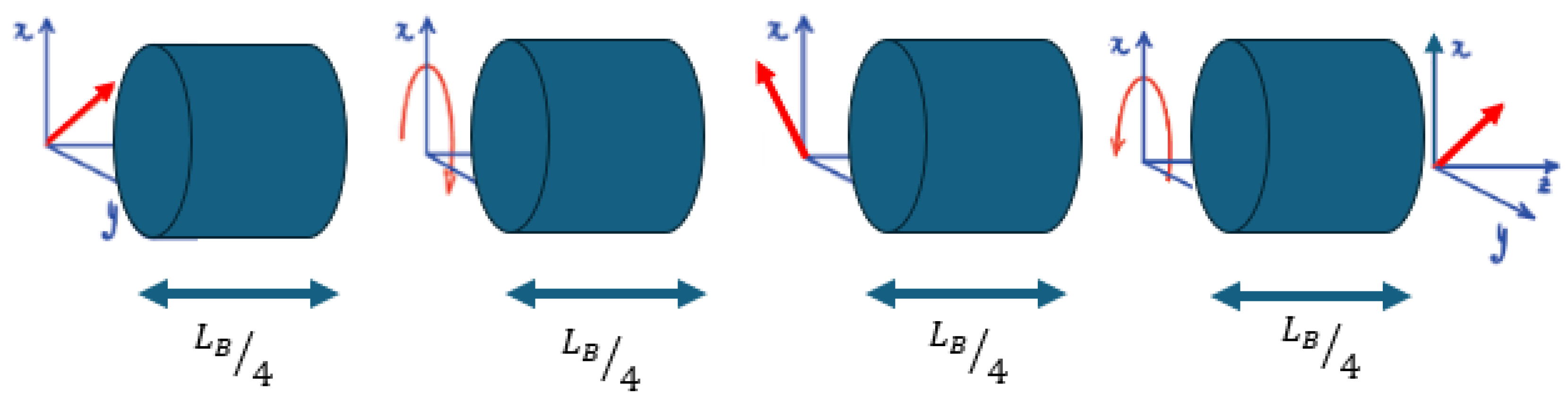
Figure 2.
Four SOP Evolution for the same Seismic Event with different set of Plates’ Angles.
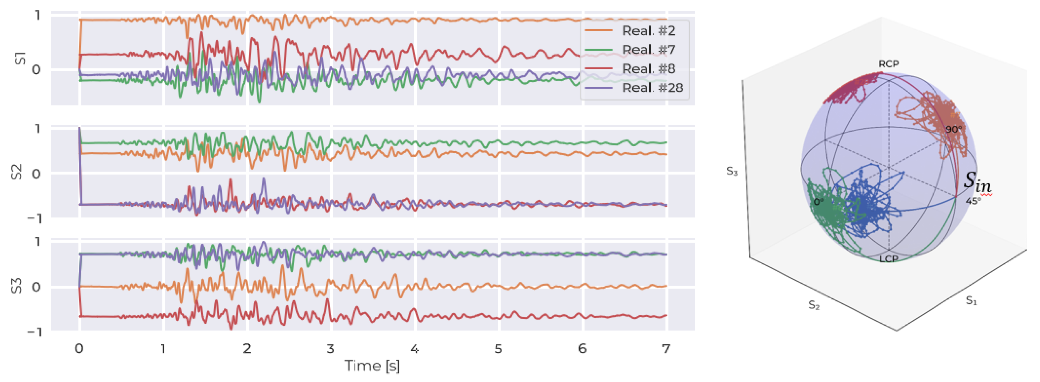
Figure 3.
ML Model Architecture.
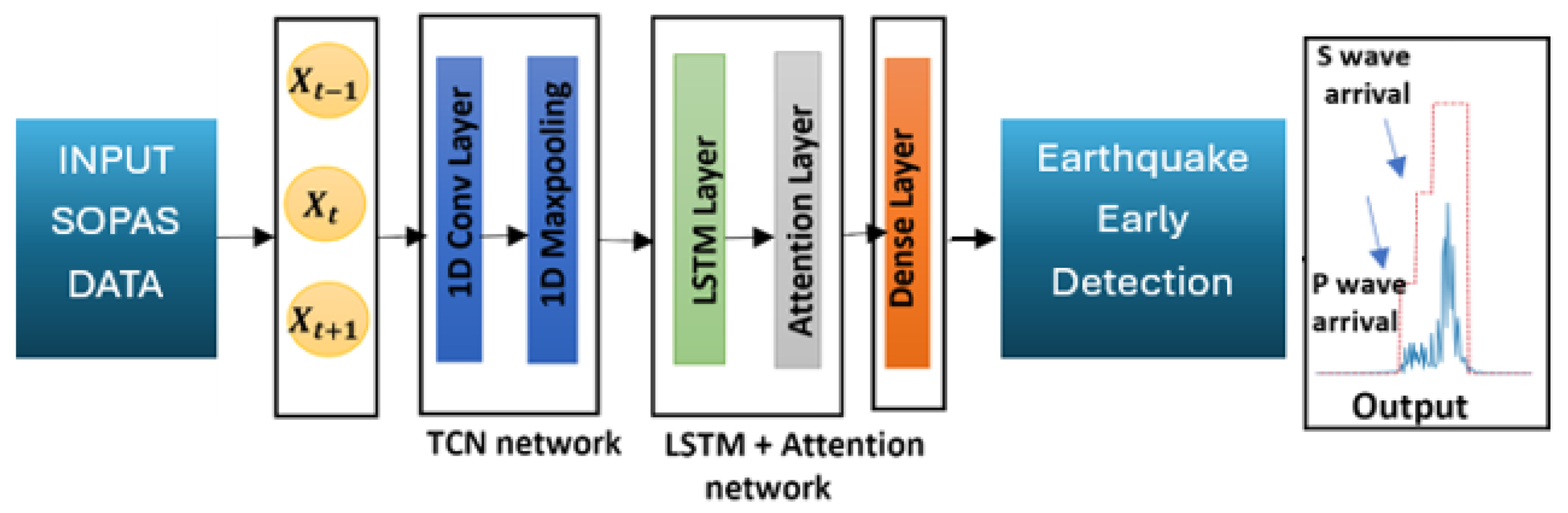
Figure 4.
ML Model Training and Validation Accuracy.

Figure 5.
M4.3 Earthquake Origin Time: 2012-05-23 21:41:18 (UTC) | Region: MODENA and corresponding Interconnected Sensing Grid in the Modena Region.
Figure 5.
M4.3 Earthquake Origin Time: 2012-05-23 21:41:18 (UTC) | Region: MODENA and corresponding Interconnected Sensing Grid in the Modena Region.

Figure 6.
Strain Evolution over T0821 Fiber - Left, MNTV Fiber - Middle, and ZCCA Fiber - Right.
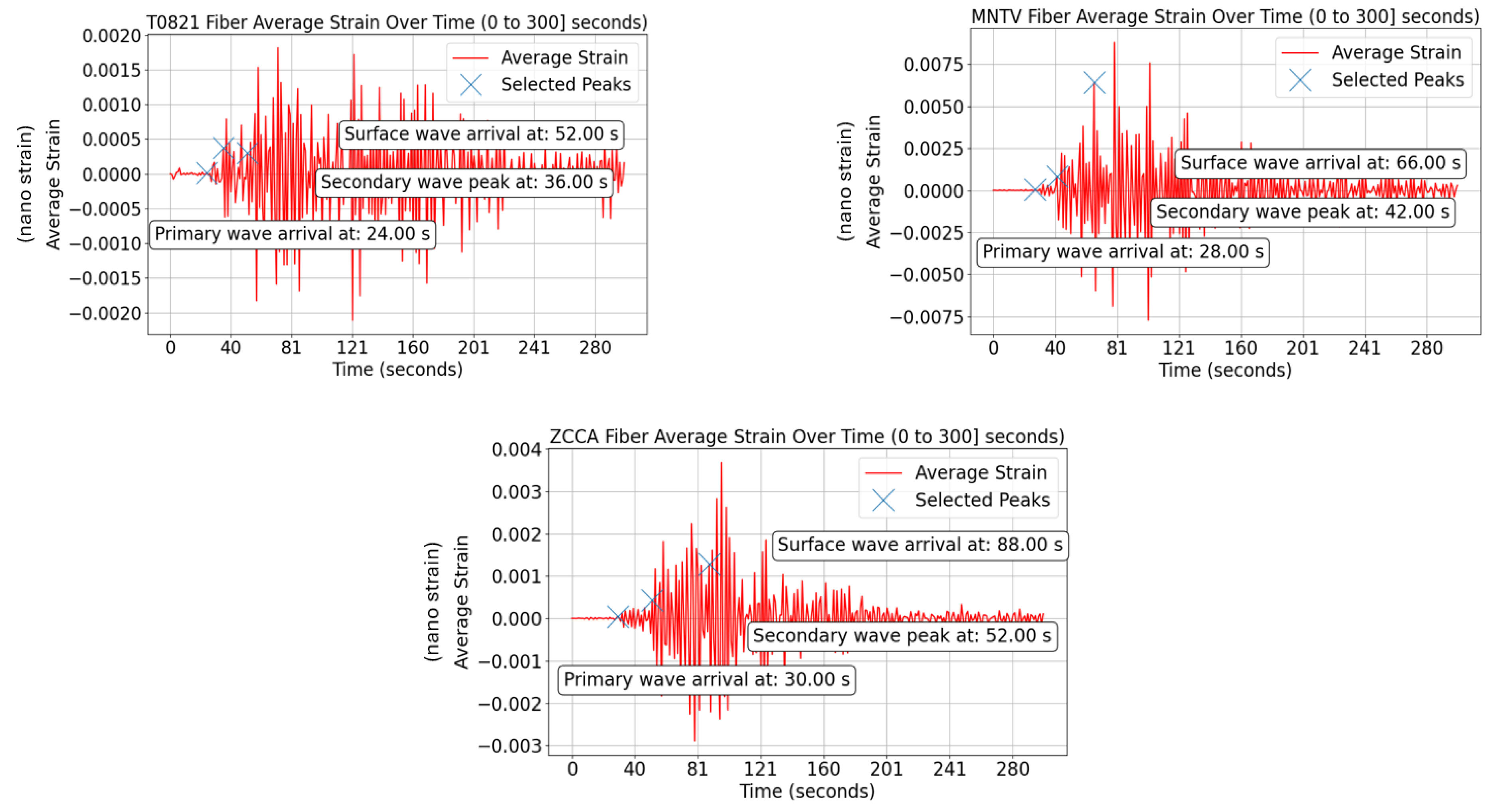
Figure 7.
SOPAS Evolution over T0821 Fiber - Left, MNTV Fiber - Middle, and ZCCA Fiber - Right.
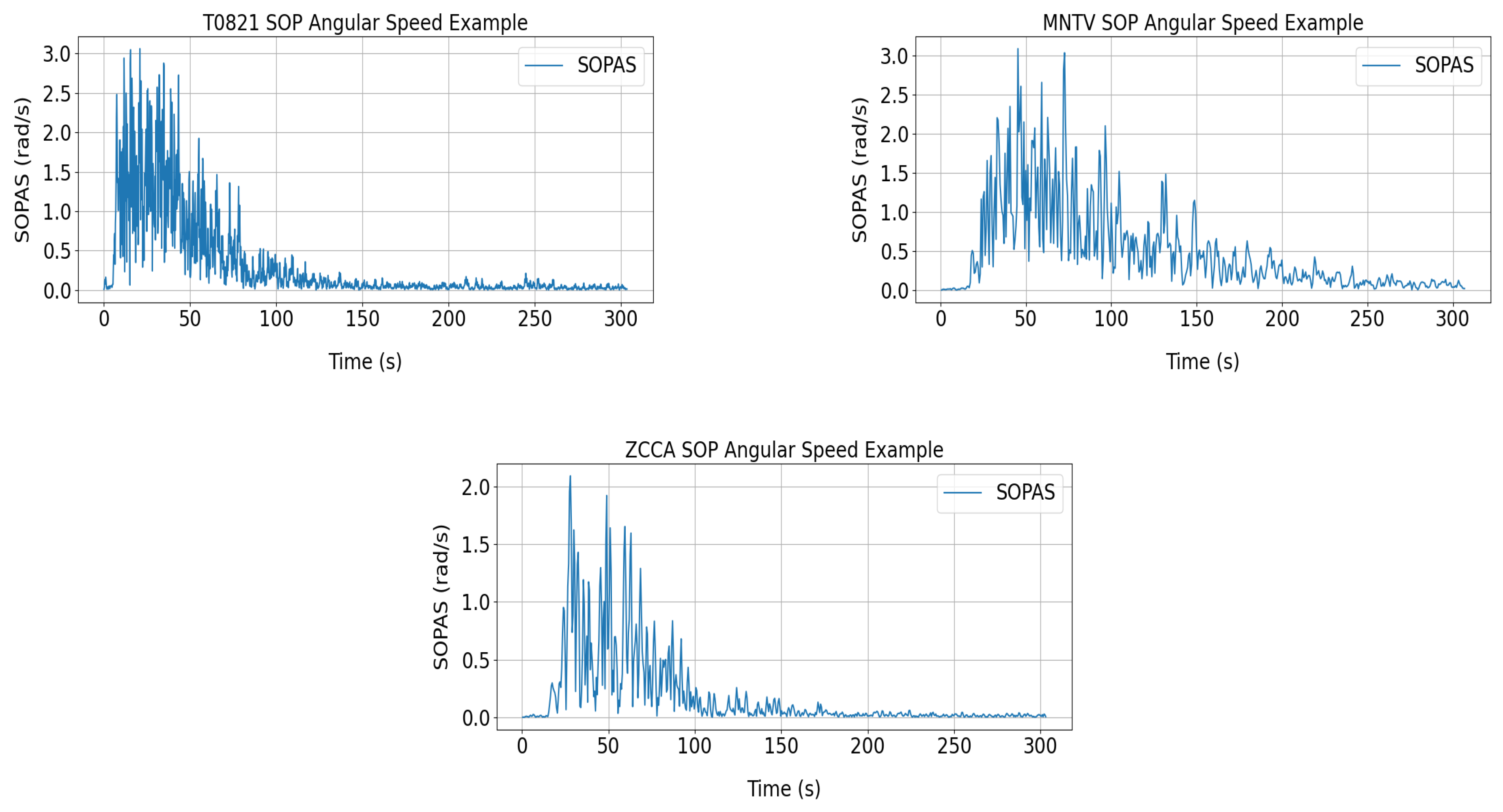
Figure 8.
Confusion Matrices over T0821 Fiber - Left, MNTV Fiber - Middle, and ZCCA Fiber - Right.
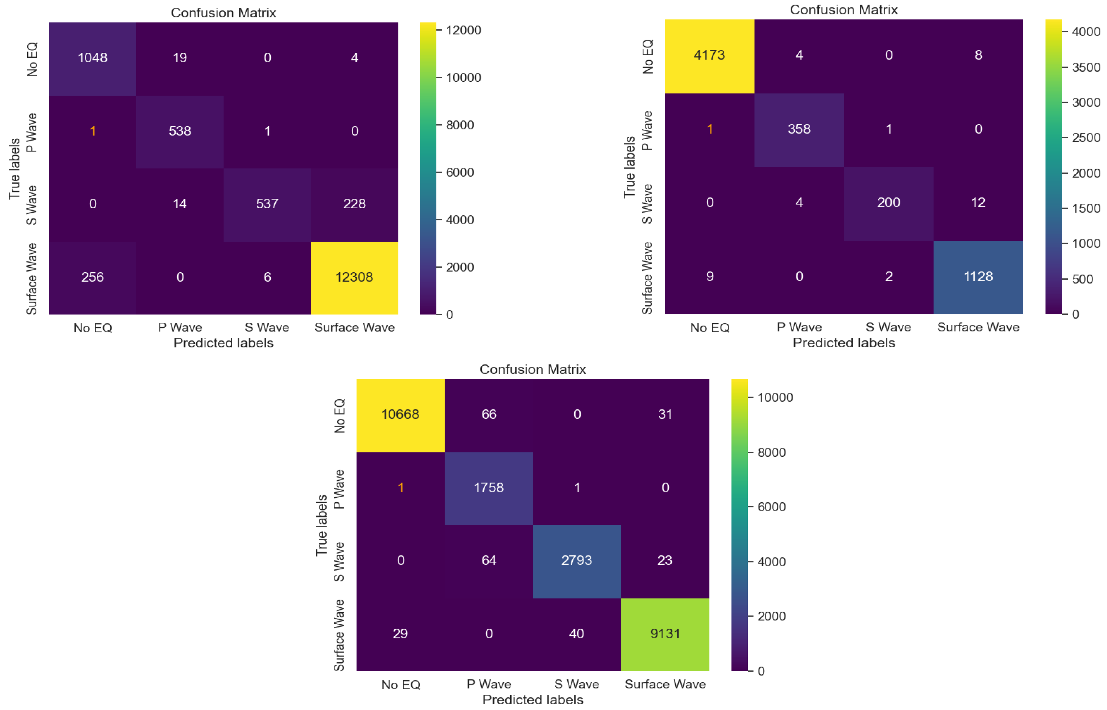
Figure 9.
ML Detection time of P Waves Using SOPAS Data Across Three Seismic Stations/Sensing-Fibers, T0821 - Left, MNTV - Middle and ZCCA - Right).
Figure 9.
ML Detection time of P Waves Using SOPAS Data Across Three Seismic Stations/Sensing-Fibers, T0821 - Left, MNTV - Middle and ZCCA - Right).
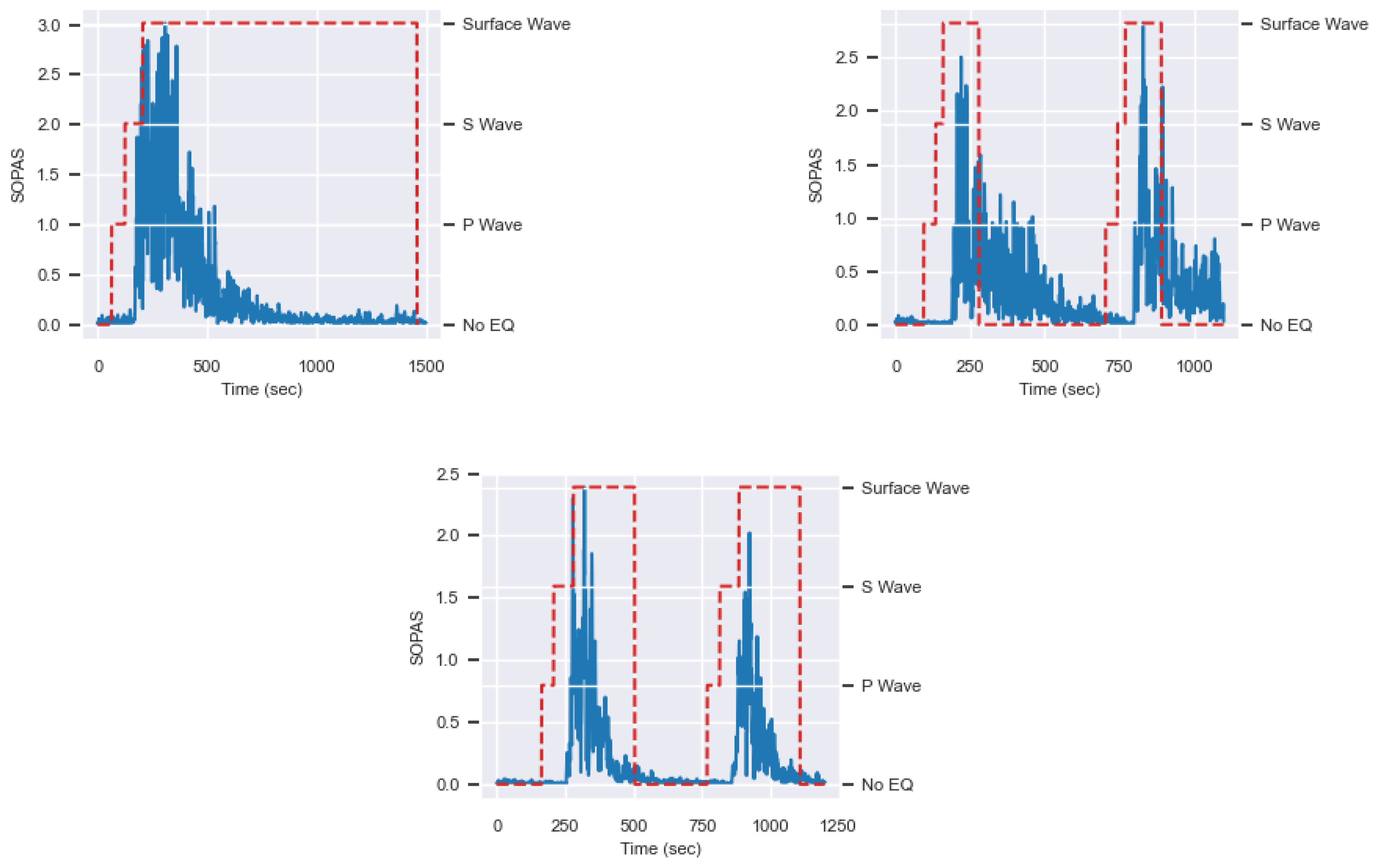

Table 1.
Comparison of epicenter locations and distances from seismic stations.
| Epicenter Location | Station to Epicenter Distance (km) | ||||
|---|---|---|---|---|---|
| Longitude | Latitude | MNTV | ZCCA | T0821 | |
| INGV Recording | 11.251 | 44.868 | 47.88 | 61.45 | 23.14 |
| Triangulation Simulator | 11.2846 | 44.8705 | 49.59 | 63.08 | 20.48 |
Disclaimer/Publisher’s Note: The statements, opinions and data contained in all publications are solely those of the individual author(s) and contributor(s) and not of MDPI and/or the editor(s). MDPI and/or the editor(s) disclaim responsibility for any injury to people or property resulting from any ideas, methods, instructions or products referred to in the content. |
© 2024 by the authors. Licensee MDPI, Basel, Switzerland. This article is an open access article distributed under the terms and conditions of the Creative Commons Attribution (CC BY) license (http://creativecommons.org/licenses/by/4.0/).
Copyright: This open access article is published under a Creative Commons CC BY 4.0 license, which permit the free download, distribution, and reuse, provided that the author and preprint are cited in any reuse.


