Submitted:
14 March 2024
Posted:
15 March 2024
Read the latest preprint version here
Abstract
Climate warming is expected to have pronounced effects on Arctic and Subarctic ecosystems, especially regions underlain by discontinuous and relatively warm permafrost. The main goal of this research is to evaluate the vulnerability and dynamics of permafrost under climate warming across the various ecotypes in respect of ecosystem stability, socioeconomic impact, and for better understanding possible future environmental changes. We suggested the new version of the spatially distributed permafrost dynamics model (GIPL2-MPI), which is developed in the Geophysical Institute, University of Alaska Fairbanks. This model is based on the ecosystem approach to simulate the permafrost dynamics, which we are discussing in this paper. We combined ground-based observations and numerical freeze/thaw modeling using climate-ecosystem-permafrost interactions to understand the physical processes and mechanisms controlling permafrost physical state. We predict the changes in permafrost conditions using output from two GCMs (NCAR-CCSM4 and GFDL-CM3) and Five-Model Average Ensemble for the RCP-4.5 and RCP-8.5 scaled down to 1 by 1 km spatial resolution (https://uaf-snap.org/) across entire Alaska. Our result shows that by the end of the current century widespread near-surface permafrost degradation could begin everywhere in Alaska southward of the Brooks Range as well as across some spots at the North Slope Alaska.
Keywords:
Permafrost
; Active Layer
; Permafrost Dynamics
; Climate Change
; Ecosystem
; Numerical Modeling
; Soil Thermal Properties.
1. Introduction
Recent observations indicate a warming of permafrost in many northern regions with a resulting degradation of ice-rich and carbon-rich permafrost. In the last 30-40 years, warming in permafrost temperatures observed in the Northern Hemisphere has resulted in the thawing of permafrost in natural, undisturbed conditions in areas both close to the southern and north boundary of the permafrost zone. The impact of climate warming on permafrost and the potential of climate feedback resulting from permafrost thawing have recently received a great deal of attention. Most of the permafrost observatories in the Northern Hemisphere show substantial warming of permafrost since the 1980s [1,2,3,4]. The magnitude of permafrost warming has varied with location but was typically from 0.5 to 4°C. A more pronounced warming has been observed in cold permafrost in higher northern latitudes and a smaller increase in temperature was typical for the warmer permafrost (because latent heat). Permafrost temperatures were stable or even slightly cooling during the last several years in the lower northern latitudes.
A comprehensive system of permafrost observatories at Alaska was established in the late 1970s and early 1980s by the Geophysical Institute, University of Alaska Fairbanks along the Trans-Alaska Pipeline and at other locations in Alaska [5,6,7,8,9].
Permafrost extent and active layer depth are very important for the high-latitude temperature regimes and water cycle. Changes in the hydrologic cycle and soil temperature can have significant consequences for local people: degrading permafrost very often could lead to ecosystem changes and threatens to damage infrastructure. Understanding how the tightly coupled permafrost and hydrology will behave in a warming world is vitally important for local communities in Alaska and throughout the circumpolar North.
Alaska is warming very fast. Therefore, there is an urgent need to develop a robust modeling tool for projecting changes associated with thawing permafrost in this region. Many important questions about present day and future ecosystems change can be answered with such tools. Even with all the uncertainty of future climate change projections this model will be useful in creating estimations of the range of future permafrost change in Alaska. Many of the proposed developments will be experimental in nature, with a final goal of providing society with robust expert assessments of changes that are important for infrastructure for several decades ahead.
Climate warming is expected to have pronounced effects on high latitude ecosystems, especially regions underlain by warm permafrost such as the Interior of Alaska [10,11,12,13]. Large areas of permafrost in Alaska have been degrading for some time [14,15] and are expected to continue to do so as the global climate warms. These changes in permafrost distribution have dramatically affected the ecosystems across Alaska through widespread drying or wetland expansion [14,15,16].
In the discontinuous permafrost zone with ground temperatures near the freezing point, the presence of vegetation and organic soil layers strongly affect the ground thermal regime due to insulation effect. Shur and Jorgenson [17] classified permafrost according to patterns of formation and degradation in relation to climate and ecosystems. They propose five main permafrost zones:
- 1)
- ‘Climate-driven’.
- 2)
- ‘Climate-driven, ecosystem-modified’.
- 3)
- ‘Climate-driven, ecosystem protected’.
- 4)
- ‘Ecosystem-driven’.
- 5)
- ‘Ecosystem-protected’ permafrost.
Permafrost in each zone reacts differently to external disturbances. The permafrost types ‘climate-driven, ecosystem protected’, ‘ecosystem-driven’, and ‘ecosystem-protected’ are in a state of dis-equilibrium with the current climate; minimal disturbances have already caused widespread permafrost degradation [18].
During the second half of the 20th century, permafrost has been thawing within the southern part of the northern Hemisphere permafrost domain. However, recent observations documented propagation of this process northward into the continuous permafrost zone. The close proximity of the exceptionally ice-rich soil horizons to the ground surface (Figure 1), which is typical for the arctic tundra biome, and loess sediments in interior Alaska makes tundra surfaces extremely sensitive to the natural and human-induced changes that resulted in development of processes such as thermokarst, thermal erosion, and retrogressive thaw slumps that strongly affect the stability of ecosystems and infrastructure. The most significant impact on ecosystems, infrastructure, carbon cycle and hydrology will be observed in areas where permafrost contains a considerable amount of ground ice in the upper few meters. Permafrost thawing is already causing serious damage to buildings and industrial facilities and is projected to continue. A major threshold is crossed when permafrost thaws after damage or removal of vegetation and upper soil organic layers, e.g., by wildfires as naturally or human activities artificially. Current permafrost temperature measurements indicate a relatively continuous warming of permafrost in most regions of Alaska over the last 30 years [2,3,9], increasing the sensitivity and vulnerability of permafrost in many regions to surface disturbances. Numerical models predict widespread warming and degradation of discontinuous permafrost until 2100, i.e., in interior Alaska. Permafrost degradation due to thermokarst processes is found in a broad variety of land surface features [15,19]. Future climate scenarios predict a roughly 2°C - 5°C increase in mean annual surface air temperature for the Alaskan Interior over the next 80 years [19]. This temperature increase will be enough to initiate permafrost degradation in interior Alaska [6,15,16,21,22], leading to widespread thermokarst development, groundwater-surface water interactions, and a deepening of seasonally thawed (active) layer [6,15,17,19].
Recently, several permafrost models were developed for various regions [21,22,23,24,25,26,27,28,29]. In many of the permafrost models, properties for the mineral and organic soil layers [21,22,24,30] or properties for the sediment and bedrock material [26], or values of n factors and thermal properties of the ground material [31] are producing a large number of distinct combinations of the input data set classes, the parameterization of which is a difficult task involving various assumptions and data sets. In some publications, the texture of mineral soils and other input parameters are used [28].
In this manuscript, we consider the ecosystem types and set of existing ground temperature observations across the individual ecosystem types. This combination allows estimation of the soil properties using the data assimilation technique for each input-data class to Alaska. The justification of this approach is based on the analysis of spatial and temporal variability of near-surface ground temperatures measured across entire Alaska [2,3,5,6,7,9,16].
To verify the developed model, we simulate the retrospective permafrost evolution and compare it with in situ observations of the active layer thickness. Consequently, we project the modeling results into the future according to the Intergovernmental Panel on Climate Change (IPCC) Representative Concentration Pathways (RCPs) 4.5 and 8.5 greenhouse gas emission scenarios [32,33,34]. The technology developed in this study is believed to be relevant and applicable to many Alaskan and other Circum-Arctic locations for the estimation of possible consequences of permafrost degradation in the 21st century.
The modes of permafrost degradation are highly variable, and its topographic and ecological consequences depend on the interactions of slope positions, soil texture, hydrology, ice content and others. However, it is still not clear how surface conditions could affect the hydrothermal dynamics of permafrost and active layer, how to determine the factors that are most important in estimating for surface condition. Knowledge of processes affecting the vulnerability of permafrost in respect to ecosystems stability, infrastructures, and socio-economic impacts, provides stakeholders with information for better understanding the range of possible future changes, to help guide land management and decision-making.
2. Permafrost Dynamics Modeling: Data and Methods
2.1. Simulation Domain
We defined the computational Alaskan domain (Figure 2a) with a spatial resolution of 1 by 1 km, which covered the entire Alaska except a small part of the Aleutian Islands. For computation the chosen area consisted of 1,497,645 grid cells. Each spatial grid cell contains a 100 m in depth multilayered soil column with 160 vertical computational grid points (layers). The total 239,623,200 computational nodes.
For the model validation and observed data incorporation into the model, we used measured data from more than fifty shallow (1.2-5.0 m in depth) boreholes across entire Alaska (Figure 2b). These high-quality ground temperature measurements (precision generally at 0.01°C) are available from the beginning of 1980s to 2023 across Alaska [2,3,5,6]. Soil water content and snow depth measurements were also available at most of these locations. In addition, more than twenty relatively deep boreholes from 15 m to 100 m in depth along the Dalton Highway were available for the model validation and calibration.
2.2. Climate Forcing
We prepared the SNAP (https://uaf-snap.org/) data set as a climate forcing to drive the GIPL2-MPI permafrost model. CMIP5/AR5 selected GCM's (https://uaf-snap.org/how-do-we-do-it) scaled down to 1 km spatial resolution were used to drive the GIPL2-MPI model. We used outputs for two operating separately GCMs GFDL-CM3 and NCAR-CCSM4 as well as for a 5-ModelAverage, and for two different greenhouse gas concentration trajectory RCP4.5 and RCP8.5.
The 5-ModelAverage is the average model output from the top Five Model Average that best replicate historical climate in Alaska and the Arctic regions (NCAR-CCSM4, GFDL-CM3, GISS-E2-R, IPSL-CM5A-LR, MRI-CGCM3) [35]. The 5-ModelAverage best for: looking at general climate trends over time, as it smooths over the year-to-year and decade-to-decade variability. NCAR-CCSM4 and GFDL-CM3 are the best for the Alaska region for exploring climatic extremes or annual variability [20]. Only individual models can provide that type of information.
RCP is a greenhouse gas concentration trajectory adopted by the IPCC [12,13]. Four pathways were used for climate modeling and research for the IPCC fifth Assessment Report (AR5) in 2013 and 2014 (Figure 3). The pathways describe different climate futures, all of which are considered possible depending on the volume of greenhouse gases (GHG) emitted in the years to come. The RCPs - originally RCP2.6, RCP4.5, RCP6.0, and RCP8.5 - are labelled after a possible range of radiative forcing values in the year 2100 2.6, 4.5, 6, and 8.5 W/m2, respectively [32,33,34]. The RCP2.6 scenario was included in the RCP set to show what it would take to limit globally averaged warming to about 1°C by 2100. RCP2.6 is generally not used in presenting plausible futures because it requires such extreme mitigation that it is considered by many climate experts to be unrealistic. The RCP2.6 scenario required that after 2020, CO2 emissions would decline and become negative by 2100 (i.e., we find ways to sequester more carbon than we are emitting in 2100). Given the present increase in the rate of emissions and CO2 concentrations, a near-term stabilization and decrease of emissions is not plausible.
The RCP2.6 scenario was included in the RCP set to show what it would take to limit globally averaged warming to about 1°C by 2100. RCP2.6 is generally not used in presenting plausible futures because it requires such extreme mitigation that it is considered by many climate experts to be unrealistic. The RCP2.6 scenario required that after 2020, CO2 emissions would decline and become negative by 2100 (i.e., we find ways to sequester more carbon than we are emitting in 2100). Given the present increase in the rate of emissions and CO2 concentrations, a near-term stabilization and decrease of emissions is not plausible.

Table 1.
Two Global Climate Models (GCM) and a composite of 5-ModelAverage GSMs scaled down to 1 by 1 km spatial resolution across Alaska used for permafrost dynamics simulation [35].
Table 1.
Two Global Climate Models (GCM) and a composite of 5-ModelAverage GSMs scaled down to 1 by 1 km spatial resolution across Alaska used for permafrost dynamics simulation [35].
| Project | Center | Model | Acronym |
|---|---|---|---|
| CMIP5/AR5 | National Center for Atmospheric Research | Community Earth System Model 4 | NCAR-CCSM4 |
| CMIP5/AR5 | NOAA Geophysical Fluid Dynamics Laboratory | Coupled Model 3.0 | GFDL-CM3 |
| CMIP5/AR5 | 5-Model Averaged | Calculated as the mean of the five GCMs* | 5-ModelAverage |
* Averaged of the five GCMs: NCAR-CCSM4, GFDL-CM3, GISS-E2-R, IPSL-CM5A-LR, MRI-CGCM3
2.3. Permafrost Dynamics Model
To evaluate the vulnerability of permafrost under climate warming across the entire Alaskan domain in respect to ecosystems stability, infrastructure and socioeconomic we applied the physical process-based permafrost dynamics model developed in Geophysical Institute Permafrost Lab (GIPL) University of Alaska Fairbanks [21,22,24,25,37].
In this research, we employ the transient permafrost dynamics model GIPL2-MPI, which simulates soil temperature dynamics and the depth of seasonal freezing and thawing by solving 1D and 2D non-linear parabolic conductive heat equation with phase change using the finite difference method. The GIPL2-MPI model captures physical processes essential to robust and appropriate modeling of soil temperature dynamics, active layer thickness and talik development if so. Specifically, soil thermal properties are parameterized according to soil texture and organic matter. In this model, the process of soil freezing/thawing occurs in accordance with the unfrozen water content and soil thermal properties, which are specific for each soil layer and for each geographical location. Unfrozen water content was parameterized by power function θ(T) = ac*((Abs (Tfr-T))bc), where ac > 0, bc < 0, T is soil temperature, and Tfr is a temperature of ice fusion or freezing point depression in soil. The absolutely stable implicit difference numerical method and enthalpy formulation of the energy conservation law [38,39,40] implemented in GIPL2-MPI makes it possible to use vertical resolution without loss of latent-heat effects in the phase transition zone, even under rapid or abrupt changes in the temperature fields [21,22,23]. Additionally, GIPL2-MPI includes thermal insulation of the snow cover, and geothermal heating at the appropriately selected depth. The upwards geothermal flux applied at the base of soil column (100 m in depth) was calculated as described in [41] for each spatially distributed grid cell. The GIPL2-MPI model also incorporates an efficient algorithm to estimate soil thermal properties using in-situ temperature measurements in the active layer and in permafrost. This simplifies model calibration for specific sites. The conceptual representation of permafrost dynamics in the GIPL2-MPI Model could be expressed as:
- Numerical finite difference solution (method) of heat diffusion;
- At least 100 m in depth vertical computational domain contains 128-256 vertical grid nodes;
- Moss insulation explicitly considered;
- Organic soil insulation explicitly considered;
- Snow insulation explicitly considered;
- Effect of unfrozen water on phase change explicitly considered;
- Thermal conductivity depends on soil moisture, temperature, and unfrozen water content.
The detailed description of the physical model and numerical solution are presented in the Appendix A.
2.4. The Ecosystem Approach of Permafrost Modeling
Definition: The ecosystem approach of permafrost modeling is based on field studies of the upper layers of soil section for various classes of ecosystems and incorporating this data into the permafrost model. For each ecosystem type the soil texture and thickness of the organic matter and mineral soil layers are parameterized according to field measurements and geographic location. In the frame of this method, the ecosystem types, and groups of existing ground temperature observations across the various ecosystem types are considered. This grouping allows estimating the soil properties using the data assimilation technique [37,50] and model validation for each input data class. An example to apply the ecosystem type approach to model permafrost across the North Slope of Alaska was presented in [24].
The 2018 Alaska Vegetation and Wetland Composite (AKVWC) represents the best-available data derived from 28 regional land cover maps that have been developed within the last 31 years (Figure 4b). The map is attributed with a uniform, two-tiered legend so that land cover classes that are similar in concept were used for determination of surface vegetation conditions, existence of organic matter and for prescribing of upper organic layers thermal properties (Figure 4a). The Alaska Land Carbon and Wetland Distribution Map (Figure 4b) was produced as part of the USGS Land Carbon Alaska assessment [42,43,44] and used for prescription of initial soil moisture content and thermal properties as well. The 2018 AKVWC data was used as one of the input datasets to the GIPL2-MPI model. The methods used to produce this wetland map as well their accuracy assessment is presented in He et al. [42]. This product was to provide regional estimates of specific wetland types (e.g. bog and fen) in Alaska, available wetland types mapped by the National Wetlands Inventory (NWI) program were reclassified into bog, fen, and other.
The map of ground ice distribution [36] was used for additional information to compile the initial soil ice/water content (Figure 6a). Ground ice volumes were estimated for the upper 5 m of permafrost using terrain relationships established by Kreig and Reger [48] and our field data. Variable ice (the legend component on the map) associated with buried glacial ice [36]. Ground ice volume near the surface is higher in colder regions due to active ice-wedge formation and ice segregation in fine-grained sediments. Buried glacial ice in old or stagnant young moraines is included but is irregularly distributed at this map scale. Depth to bedrock was used to compile the deep soil column structure in terms of the thickness of fine-grained soil layers or depth to bedrock (Figure 6b).
2.5. Data Assimilation and Model Validation
Different earth materials have varying thermal properties. The soil thermal conductivity and heat capacity vary within different soil layers as well as during thawing/freezing cycles and depend on the unfrozen water content that is a certain function of temperature. The method of obtaining these properties is based on numerical solution for a coefficient inverse problem and on minimization locally the misfit between measured and modeled temperatures by changing thermal properties along the direction of the steepest descent. The method used and its limitations are described in more detail elsewhere [21,22,37].
For the initial model calibration, we used data from more than fifty shallow boreholes (1-1.5 m in depth) across Alaska from north to south. These high-quality ground temperature measurements (precision generally at 0.01°C) are available from the beginning of 1980s to 2022 across Alaska [5,6,9]. Soil water content and snow depth measurements were also available at most of these boreholes. The temperature measurements in the shallow holes were performed with vertical spacing of 0.08-0.15 m. At most of these sites, soil water content and snow depth were also recorded. In addition, more than twenty relatively deep boreholes from 15 m to 100 m in depth along the same transect (Figure 7a) were available for the model validation in terms of permafrost temperature profiles, active layer depth and permafrost thickness. Figure 7 illustrates the results of the GIPL2-MPI model calibration for the West Dock (WD) permafrost observatory. The specific site WD is classified as an Arctic Tundra (70°22’28.08” N, 148°33’7.8” W). Reconstructed soil thermal properties for the WD site (Arctic Tundra) and other major ecotypes are shown in Table 2.
There are two basic approaches to calibration of modeled permafrost temperatures against the observed data, which can be distinguished by their use of temporal or spatial relationships. With the temporal approach, the quality of the modeling series is assessed by time series regression against measured data Figure 7b, Figure 8b, Figure 9b and Figure 10b. The quantitative relationship between simulated and measured data is then determined for a ‘‘calibration’’ period with some instrumental data withheld to assess the veracity of the relationship with independent data.
In the spatial approach, assemblages of the observed data from several different geographic locations with different landscape settings determine the quality of the modeling results. To achieve geographic correspondence between the scale of observation and modeling we utilized a regional scale permafrost characterization based on observations obtained from representative locations. Additional comparison of model produced ground temperatures, active layer thickness, and spatial permafrost distribution with measured ground temperatures at the Alaska sites shows a good agreement e.g. Figure 7b, Figure 8b, Figure 9b and Figure 10b.
Here we followed the idea of the variational approach and optimized a set of model parameters by minimizing difference between the observed and modeled soil temperature [37,50]. This task was associated with estimation of thermal properties of the ground material. Results of previous investigations [4,48] were used to determine the initial approximation to the model parameters. The soil characterization used in the GIPL2-MPI model was based on extensive empirical observations, conducted in representative locations that are characteristic for the major physiographic units across entire Alaska. Once the initial approximation was defined, we varied the set of parameters associated with the ground material in order to decrease the discrepancy between the simulated and observed temperature climatology at all other depths below the surface. Hence, at each step of the minimization procedure, if the quantity of parameters was updated, we recomputed the ground temperature dynamics for all relevant sites. After a few iterations, we obtained values for the ground thermal properties for the 26 ecotypes and soil classes for Alaska. Some year-to-year differences between the modeled and observed annual cycles exist. However, in general, the modeled and observed ground temperature climatology agree well with each other as shown in Figure 7b, Figure 8b, Figure 9b and Figure 10b. The error is typically less than 0.328°C, except when the snowmelt occurs. Some water may potentially penetrate into the borehole and may warm the sensors.
2.5.1. Model Validation
Model validation usually comes down to the process of comparing model simulations to an experimental or observed data set. Comparison with a real data set is the most reliable and preferred way to validate a simulation model.
The result of modeled and observed MAGT and ALT comparison confirmed that the model is predictive under the conditions of their intended use and satisfactorily reflects the real permafrost conditions across the entire Alaska (Figure 11). The averaged values of MAGT and ALT are simulated over the various periods of time between 1997 and 2017. There is some degree of inaccuracy, but generally, the modeling results demonstrate that the model is a reasonable representation of the actual permafrost environment and in very good agreement with observed data.
2.6. Sensitivity Analysis
Uncertainties in the presented model lie in specifying the thermal parameters such as heat capacity of frozen and thawed soils and thermal conductivity. But mostly uncertainties are affected by thermal conductivity and the volumetric soil moisture content. The employed values for the soil properties are recovered by assimilating in situ temperature observations at a series of the Geophysical Institute, UAF and USGS sites across Alaska. The model is verified by comparing with available active layer thickness at the Circumpolar Active Layer Monitoring (CALM) sites (https://www2.gwu.edu/~calm/), perma-frost temperature, and snow depth records from existing permafrost observatories in the Alaska North Slope region. These data sets may contain some biases and errors, and hence, to gain some knowledge about how they act together and influence the results. We conducted a sensitivity analysis for a typical permafrost observing station at the region of discontinuous permafrost distribution. For a few other locations within continuous and sporadic permafrost regions, we obtained similar results.
For the Smith Lake station, a station with a typical natural condition black spruce ecosystem at the interior Alaska region, we analyze sensitivity of the mean annual ground temperature (MAGT) at 1 m depth and active layer thickness (ALT) with respect to the volumetric soil moisture content, thermal conductivities of thawed and frozen soils between 0.25 and 1.0 m depth (Figure 12b–d) and surface conditions such as moss and upper organic layer (Appendix B). Our previous investigations showed that variations in the heat capacities frozen and thawed soils do not significantly affect the modeling results for ALT and MAGT [21,37,51,52]. The obtained sensitivity results for thermal conductivity, both thawed and frozen soils are shown in Figure 12c, d. As the MAGT increased, the depth of the ALT increased as well.
The most influence on the average values of ALT and MAGT is imposed by the values of thermal conductivity of thawed soils within the 0.25-1.0 m depth (Figure 12c). The most impact on the MAGT is imposed by the values of thermal conductivity of unfrozen and frozen soils for the soil layers between 0.5 m and 1 m in depth. The value of frozen conductivity affects the soil layer below 1 m, and soil water content for the layer between 0.5-1.0 m soil layers. Values of the thermal conductivity for the upper layers are the primary function of the organic matter content and soil moisture. Additional illustrations on the model sensitivity to surface conditions, for example presence or absence of moss and organic matter at the upper part of the soil column are provided in Appendix B.
3. Discussion
The modeling result shows the most significant changes in the upper layer (0.2-5.0 m) of ground temperature, active layer thickness as well as talik development, occurred under the climate scenario provided by the GFDL-CM3 climate model both 4.5 and 8.5 RCPs. As described by the IPCC the RCP-4.5 is an intermediate scenario [12,13]. Increase in soil temperature in RCP-4.5 peak around 2051-2070, then observed relative decline. RCP-4.5 is more likely than not to result in global temperature rise between 2.5°C and 3.5°C, by 2120 (Table 3). In RCP-8.5, ground temperature continues to rise throughout the 21st century.
The developed ecosystem approach of permafrost dynamics modeling attempts to address the problem of computing the ground temperature projections at the regional scale using the very high-resolution input dataset. It is sufficient to gain some understanding of how potential changes in permafrost could affect ecosystems and impact the infrastructure under various climate scenarios. The developed parametrization of the ground thermal properties and incorporation in-situ data into the model, which is obtained using a data assimilation technique [37,50]. Generally, the modeling results very well agree with observations.
We run the GIPL2-MPI permafrost dynamics model in order to project permafrost dynamics for the specific sites located along the Alaskan Permafrost-Ecological Transect from north to south across the entire Alaska. The modeling ground temperature dynamics at 2 m depth during 2021-2120 according to the Five-Model Average climate forcing illustrated Figure 13.
According to the modeling result the time in the calendar years of the 0°C threshold crossing of MAGT at 2 m depth generally decreases from north to south (Figure 13). It means at the south of Alaska the soil temperature crosses zero Centigrade threshold earlier in comparison with northern part of Alaska. An exception may be the Gulkana observing site, located near the southern border of the discontinuous permafrost distribution at the south of Alaska as well (Figure 7b). Here, a zero curtain at 2 meters depth could exist around between 2020 and 2090 according to Five-Model Average of the RCP-4.5 scenario (Figure 13a) and between 2020 and 2075 if climate change occurs in accordance with RCP-8.5 scenario (Figure 13b). These circumstances can be explained that the borehole located at the Copper River Basin within the area of the former Late Pleistocene ice-rich (up to 40-60%) glacial-lacustrine sediments [59,60,61,62]. Our permafrost observations showed that in this area the permafrost temperature varies between -0.5°C and -0.9°C. The thickness of the permafrost is 50-40 m and within the range of depths 10-30 m the permafrost is isothermal (there is no temperature gradient). This fact suggests that in some locations across this permafrost region the phase transition process is already occurring. It is very close to the research that was done in this region [59,60,61,62] and to our long-term permafrost field observations [2,3].
4. Conclusions
The developed transient model and ecosystem approach allows computation of ground temperature at various depths with daily resolution, ALT and talik development at the regional scale that are sufficient to gain understanding how probable changes in the permafrost might affect ecosystems and impact infrastructure under various climate scenarios. The developed parametrization of the ground thermal properties is obtained using a data assimilation technique [21,37,50]. The model validation and modeling results demonstrate that the model is a reasonable representation of the actual permafrost environment across the study area and in very good agreement with observed data.
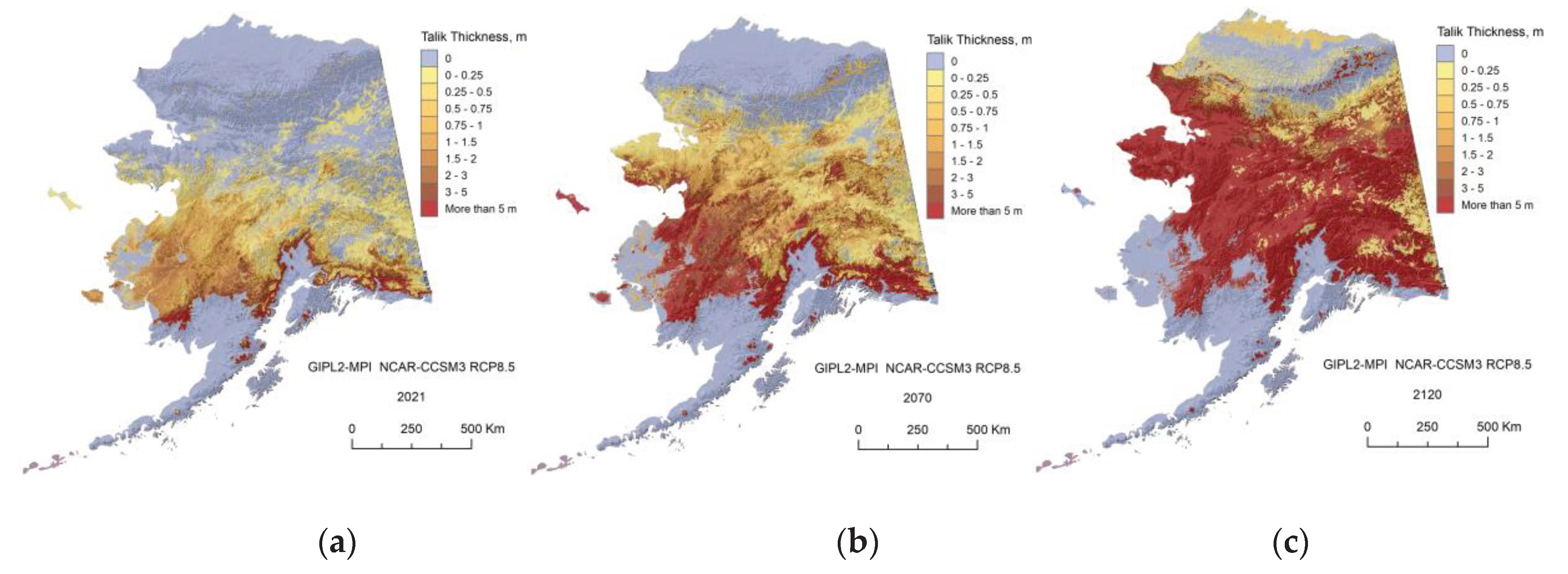
In this research, we demonstrate the projections for two GCMs and Five Models Composite for RCP-4.5 and RCP-8.5 scenarios only and illustrate a significant difference in the future near-surface ground temperature regimes between 2070s and 2110s. For the RCP-8.5 scenario, we found that ALT or top of permafrost deepening, up to 1.5 m on average in 2021, increases by a factor of 2.5 by 2070 and by a factor 3.6 from 2070 to 2120, according to the GFDL-CM3 RCP 8.5 scenario. ALT continues to increase and widespread talik starts to develop in interior Alaska and even within the individual areas of the North Slope Alaska region. According to NCAR-CCSM4 RCP-8.5 scenario the factor of permafrost top deepening increased by 1.8 from 2021 to 2070 and by the factor 3.1 from 2070 to 2120. Development of the talik will have serious implications for ecosystems, human activities (infrastructure and subsistence lifestyle), and potential feedback to climate change. On the other hand, for the RCP-4.5 scenario, the current model predicts only a modest increase in the near-surface permafrost temperatures and a limited degradation of the near-surface permafrost in the Alaska North Slope region. Finally, we mention that according to our computer experiments, in order to keep permafrost from the substantial thawing, the RCP-4.5 scenario most likely needs to be a target for greenhouse gas emissions. Appendix C illustrates the GeoTIF Maps of permafrost dynamics, generated by GIPL2-MPI using GFDL-CM3 and NCAR-CCSM4 and Five Model Average RCP-4.5 and RCP-8.5 scenarios.
5. Glossary of Permafrost and Related Ground-Ice Terms
Glossary and Comments to the Terms used in the current Report: [53,54,55,56] and Marchenko’s comments.
- Active layer - the layer of ground that is subject to annual thawing and freezing in areas underlain by permafrost.
Comment: In the zone of continuous permafrost, the active layer (seasonally freezing layer) generally reaches the permafrost table; in the zone of discontinuous permafrost, sometimes it does not. The active layer includes the uppermost part of the permafrost wherever.
- Kurum - A general term for all types of coarse clastic formations on slopes of 2-3 to 40 degrees, moving downslope mainly due to creep.
- Permafrost Table or Top of Permafrost - the upper boundary of permafrost surface.
Comment: The depth of this boundary below the land surface, whether exposed or covered by a water body or glacier ice, is variable depending on such local fac-tors as topography, exposure to the sun, insulating cover of vegetation and snow, drainage, grain size and degree of sorting of the soil, and thermal properties of soil and rock.
Comment: We used the term active layer thickness (ALT) in case of freeze-up seasonal frost with permafrost table every year. However, we are using the term ‘top of permafrost position’ or ‘table of permafrost position’ in case of the existence of residual thawed layer (talik) between seasonal frost and top of permafrost. In other words, the freeze-up does not exist anymore.
- Permafrost base - the lower boundary surface of permafrost, above which temperatures are perennially below 0°C (cryotic) and below which temperatures are perennially above 0°C (noncryotic).
- Permafrost thickness - The vertical distance between the permafrost table and the permafrost base.
- Pereletok - is a layer of frozen ground which forms as part of the seasonally frozen ground (in areas free of permafrost or with a lowered permafrost table), re-mains frozen throughout one or several summers, and then thaws.
- Protalus - A pronival rampart, formerly referred to as a protalus rampart, is de-fined as a ridge, series of ridges or ramp of debris formed at the downslope margin of a perennial or semi-permanent snow bed, which is typically located near the base of a steep bedrock slope in a periglacial environment.
- Talik - a layer or body of unfrozen ground occurring in a permafrost area due to a local anomaly in thermal, hydrological, hydrogeological, or hadrochemical conditions.
Comment: Taliks may have temperatures above 0°C (noncryotic) or below °C (cryotic, forming part of the permafrost). Some taliks may be affected by seasonal freezing. Several types of taliks can be distinguished based on their relationship to the permafrost (closed, open, lateral, isolated, and transient taliks), and based on the mechanism responsible for their unfrozen condition (hadrochemical, hydro-thermal and thermal taliks).
- Talus. - An outward sloping and accumulated heap or mass of rock fragments of any size or shape (usually coarse and angular) derived from and lying at the base of a cliff or very steep, rocky slope, and formed chiefly by gravitational falling, rolling, or sliding.
- Isolated talik - a layer or body of unfrozen ground surrounded by perennially frozen ground.
- Open talik - a body of unfrozen ground that penetrates the permafrost completely, connecting suprapermafrost and subpermafrost water.
6. Acronyms and Abbreviations
| 5-ModelAvg | Five-Model Average. Composite of five GCMs that best replicate historical climate in Alaska and the Arctic regions (NCAR-CCSM4, GFDL-CM3, GISS-E2-R, IPSL-CM5A-LR, and MRI-CGCM3). |
| AKVWC | Alaska Vegetation and Wetland Composite. |
| ALT | Active Layer Thickness. |
| AR5 | The IPCC Fifth Assessment Report. |
| ASL | Above sea level. |
| APET | Alaskan Permafrost-Ecological Transect. |
| CALM | Circumpolar Active Layer Monitoring. |
| CMIP5 | Coupled Model Intercomparison Project Phase 5. |
| CRREL | Cold Regions Research and Engineering Laboratory. |
| DEM | Digital Elevation Model. |
| DoD | Department of Defense. |
| ERDC | Engineer Research and Development Center. |
| FMA | Five-Model Average. |
| GCM | General Circulation Model. |
| GFDL-CM3 | Geophysical Fluid Dynamics Laboratory Climate System Model. |
| GHG | Greenhouse gases. |
| GI | Geophysical Institute. |
| GIPL | Geophysical Institute Permafrost Lab. |
| GIPL2-MPI | The Geophysical Institute Permafrost Lab Permafrost Dynamics Model of the Second Generation, Parallel-coded using the Message Passing Interface. |
| GIS | Geographic Information System. |
| GTN-P | Global Terrestrial Network for Permafrost. |
| HPC | The high-performance computing. |
| HPCC | High Performance Computing Center. |
| IPCC | Intergovernmental Panel on Climate Change. |
| LTER | Long Term Ecological Research Network. |
| MAAT | Mean annual air temperature. |
| MAGT | Mean annual ground temperature. |
| MMGT | Mean monthly ground temperature. |
| MPI | Message Passing Interface. |
| NWI | National Wetlands Inventory |
| NCAR-CCSM4 | National Center for Atmospheric Research Community Climate System Model. |
| pfTop | Table of Permafrost (top of permafrost). |
| RCSG | Research Computing Systems Group. |
| RCS | Research Computing Systems. |
| RCP | A Representative Concentration Pathway is a greenhouse gas concentration trajectory adopted by the IPCC. Four pathways were used for climate modeling and research for the IPCC Fifth Assessment Report in 2014. |
| RGM | Regional Climate Model. |
| SERDP | Strategic Environmental Research and Development Program. |
| SNAP | Scenarios Network for Alaska and Arctic Planning. |
| UAF | University of Alaska Fairbanks. |
| USARAK | United States Army Alaska. |
| USGS | United States Geological Service. |
| VWC | Volumetric Vater Content. |
Appendix A. The GIPL2-MPI Physical Model
A1. Mathematical Formulation
Here we proposed the mathematical problem statement, the numerical solution for the nonlinear equations of conduction heat flow. This part of calculation uses only the conductive mechanism of heat transfer. The model takes into account the latent heat of ice formation-fusion in the ground. Heat conduction in the solid soil is determined by numerically solving the second law of heat conduction equation.
where (1) is a nonlinear equation of conduction heat transfer, (2) and (3) are upper boundary conditions and initial conditions respectively, where φ is initial distribution of temperature with depth z. Dirichlet’s conditions T(τ) were set at the upper boundary. (4) Are the lower boundary conditions. At the lower boundary dn=100 m of the vertical computational domain an empirical method of geothermal heat flux estimating [41] was applied for each spatial grid cell. q(τ) is a temperature gradient [°C/m] or heat flux [W/m*K]. T
is a soil temperature at the current iteration. Tα is the near-surface
air temperature, λ is the thermal conductivity of ground, C(z, T) is a
volumetric heat capacity; z and τ are vertical and temporal axes respectively.
R is the radiation balance of a surface and determined as R = Qsun(1-A), where
Qsun is the incoming solar radiation; A is the albedo of the surface. Usually,
albedo is determined by A = S/Qsun, where S is reflected radiation. L is the
latent heat of water evaporation and E is turbulent moisture flux. Factor f(τ)
is the factor of heat exchange with snow and surface vegetation cover and α0 is
a convection heat transfer coefficient taking into account heat exchange at the
boundary snow-surface of ground or vegetation:
Heat transport in snow is largely dependent on the microstructure of the snow (pore and grain distribution and size) which is difficult to quantify [57], particularly for continental-scale simulations. The thermal conductivity of snow is therefore often calculated using empirical functions that are based on measurable properties of snow. We used the empirical equation of Proskuryakov [58], which calculates the heat flux through the snowpack into the soil as a function of snow depth Dsnow [m] and snow density [kg/m−3]:
where set to 20.14 (W/(m*K)) is the averaged factor of convection heat exchange at the surface of snow and is the snow thermal resistivity. The thermal conductivity increases with increasing snow density and is therefore higher later in the snow season.
Q(z) is the latent heat of ice formation/fusion in the ground and δ(T) is the Dirac delta function having the following properties:
where is the width of a half-interval of smoothing volumetric heat
capacity and the smoothed thermal conductivity . The smoothing
range of soil properties is set to 0.08°C. T*(z) the freezing point of
groundwater. The latent heat of ice formation-fusion is therefore represented
through apparent volumetric heat capacity at the phase
plane T(z, τ)=T*(z) so that the heat transfer problem can be solved
without explicit representation of freezing front coordinates.
The initial temperature distribution with depth is given by a piecewise linear or segmented function from the solution of the stationary problem for a multilayer medium:
λi - is a thermal conductivity of the i-soil layer at the boundary between the soil layers; λi must satisfy to the conditions of ideal contact (8, 10):
A2. Numerical Implementation
For the numerical solution of equations (1)-(4) a finite difference method was used [38,39,40]. The explicit finite difference numerical method has the second approximation order of O(h2+Δτ), where h and Δτ are vertical (depth) and temporal steps respectively.
With the second order of accuracy in depth and the first order in time, (1) approximated by a two-layered implicit finite-difference method/scheme:
The volumetric heat capacity approximated as follows:
The thermal conductivity approximated as follows:
Appendix B. Sensitivity Analysis: Model Sensitivity to Surface Conditions and Organic Matter
Figure B1.
Mean monthly contemporary air temperature (MMAT) with no trend during the 420 months used as a climate forcing for the sensitivity analysis of the GIPL2-MPI model in respect to perform the sensitivity analysis of surface conditions and organic matter impact.
Figure B1.
Mean monthly contemporary air temperature (MMAT) with no trend during the 420 months used as a climate forcing for the sensitivity analysis of the GIPL2-MPI model in respect to perform the sensitivity analysis of surface conditions and organic matter impact.
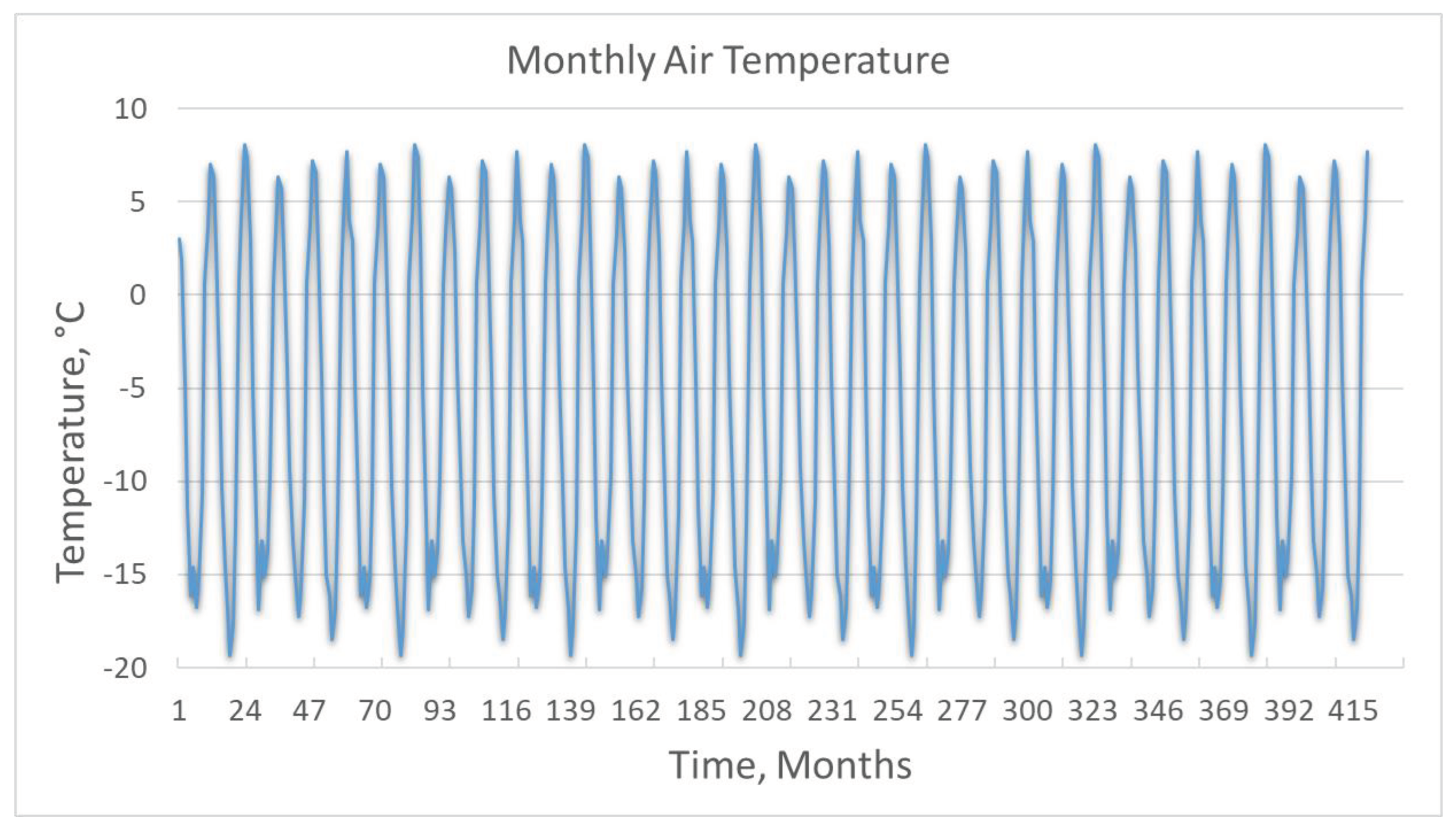
Table B1.
Soil physical properties used for permafrost dynamics simulation and model sensitivity analysis in respect to surface conditions and impact of organic matter to ALT and below-ground temperature.
Table B1.
Soil physical properties used for permafrost dynamics simulation and model sensitivity analysis in respect to surface conditions and impact of organic matter to ALT and below-ground temperature.
| Bottom of the Soil Layer’s, m | VWC | Cond th | Cond fr | Cap th | Cap fr | Thickness (m) and description of the soil layer | |
|---|---|---|---|---|---|---|---|
| 0.12 | 0.571 | 0.321 | 0.943 | 1.83d6 | 1.32d6 | 0.12 | Moss |
| 0.22 | 0.542 | 0.442 | 0.987 | 1.95d6 | 1.46d6 | 0.1 | Peat 1, fibrous, remains of grass root |
| 0.68 | 0.514 | 0.612 | 1.213 | 2.85d6 | 2.32d6 | 0.46 | Peat 2, amorphous |
| 2.68 | 0.456 | 1.023 | 1.354 | 2.95d6 | 2.42d6 | 2.0 | Mineral soil 1, silt, fine-grained soil |
| 8.8 | 0.398 | 1.232 | 1.567 | 3.17d6 | 2.73d6 | 6.12 | Mineral soil 2, silt, fine-grained sand |
| 48.5 | 0.351 | 1.324 | 1.621 | 2.89d6 | 2.38d6 | 39.7 | Mineral soil 3, clay, silt, sand |
| 52.0 | 0.323 | 1.654 | 1.978 | 3.26d6 | 2.75d6 | 3.5 | Gravel, coarse sand, coarse debris |
| 100.0 | 0.075 | 3.204 | 3.298 | 3.53d6 | 2.93d6 | 48.0 | Bedrock 5% cracks |
VWC – volumetric soil water content. Cond (th, fr) – thermal conductivity of thawed and frozen soil respectively (W/mK). Cap (th, fr) – heat capacity of thawed and frozen soil respectively (J/m3K).
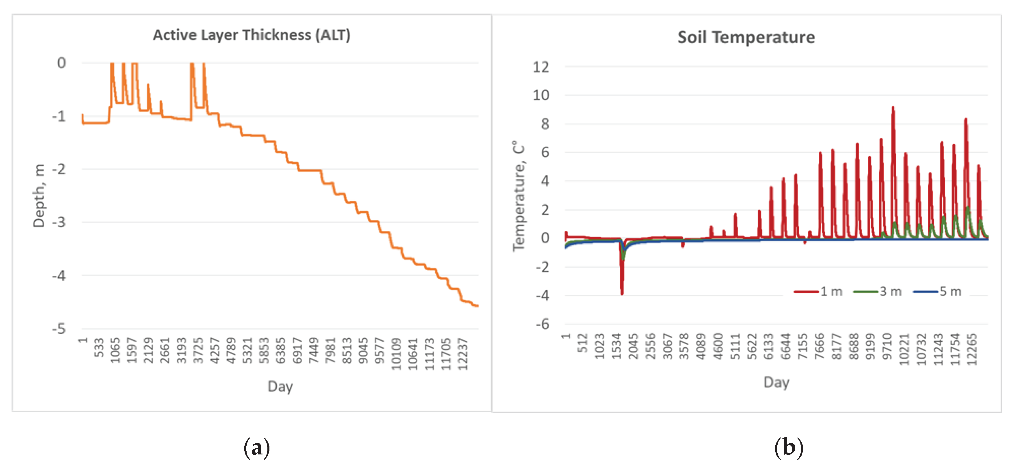
Figure B2.
(a) ALT dynamics and (b) daily soil temperature at various depths (1 m, 3 m, and 5 m depths) under undisturbed surface conditions: moss, peat 1 (fibrous), peat 2 (amorphous) are existing at the top of soil column (Table B1).
Figure B2.
(a) ALT dynamics and (b) daily soil temperature at various depths (1 m, 3 m, and 5 m depths) under undisturbed surface conditions: moss, peat 1 (fibrous), peat 2 (amorphous) are existing at the top of soil column (Table B1).
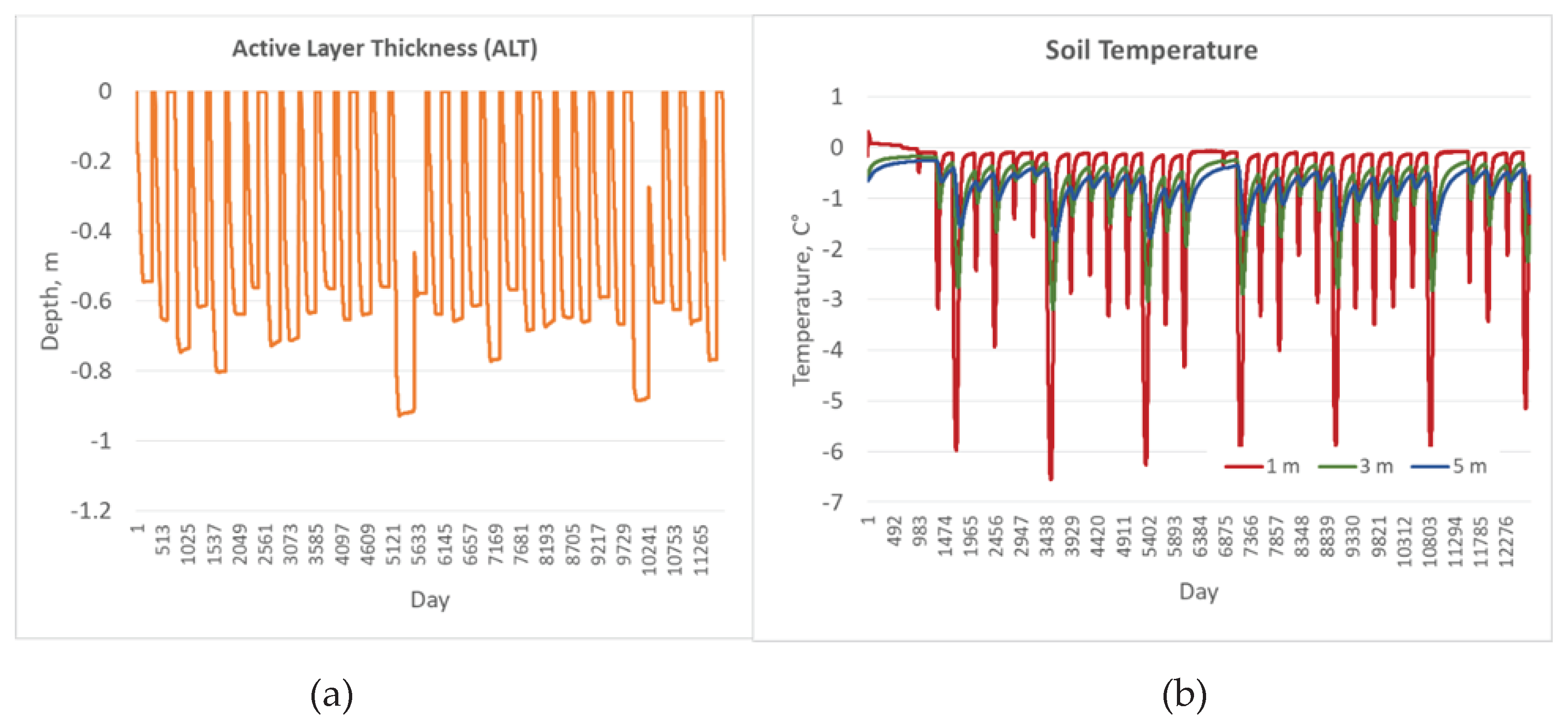
Figure B3.
(a) ALT dynamics and (b) daily soil temperature at various depths under disturbed surface conditions: no moss; but peat 1 (fibrous) and peat 2 (amorphous) are existing above silt and other soil layers are forming the soil column (Table B1).
Figure B3.
(a) ALT dynamics and (b) daily soil temperature at various depths under disturbed surface conditions: no moss; but peat 1 (fibrous) and peat 2 (amorphous) are existing above silt and other soil layers are forming the soil column (Table B1).
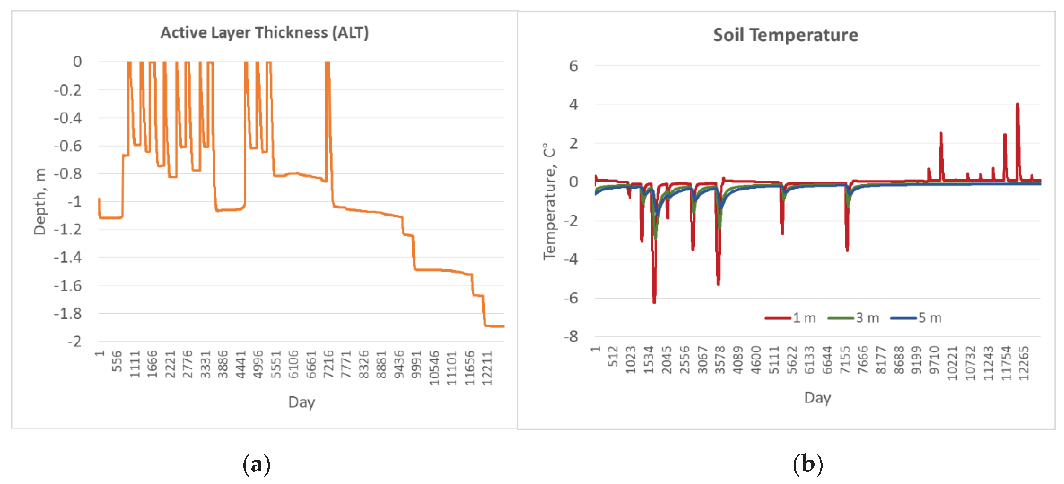
Figure B4.
(a) ALT dynamics and (b) daily soil temperature at various depths under disturbed surface conditions: no moss, no peat 1 (fibrous), but peat 2 (amorphous) are still existing above silt and other soil layers, which are forming the soil column (Table B1).
Figure B4.
(a) ALT dynamics and (b) daily soil temperature at various depths under disturbed surface conditions: no moss, no peat 1 (fibrous), but peat 2 (amorphous) are still existing above silt and other soil layers, which are forming the soil column (Table B1).
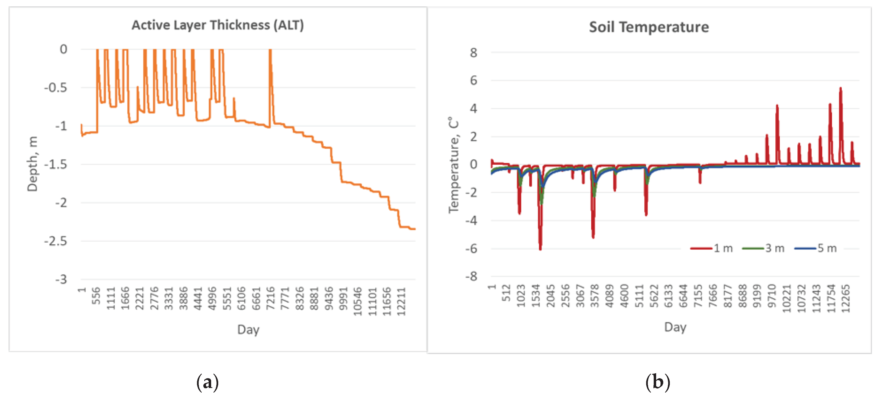
Figure B2.8.
(a) The ALT dynamics and (b) daily soil temperature at various depths under disturbed surface conditions: no moss, no peat 1 (fibrous), no peat 2 (amorphous) above silt and other soil layers, which are forming the soil column (Table B1).
Figure B2.8.
(a) The ALT dynamics and (b) daily soil temperature at various depths under disturbed surface conditions: no moss, no peat 1 (fibrous), no peat 2 (amorphous) above silt and other soil layers, which are forming the soil column (Table B1).
Appendix C. Result of the GIPL2-MPI Spatial and Temporal Permafrost Dynamics Modeling During 2021-2120: GeoTIF Digital Maps
Figure C1.
The GIPL2-MPI modeled MAGT at 2 m depth for 2021 (a), 2070 (b) and 2120 (c) snap shots using 5-Model Average composite RCP-4.5 as a climate forcing.
Figure C1.
The GIPL2-MPI modeled MAGT at 2 m depth for 2021 (a), 2070 (b) and 2120 (c) snap shots using 5-Model Average composite RCP-4.5 as a climate forcing.
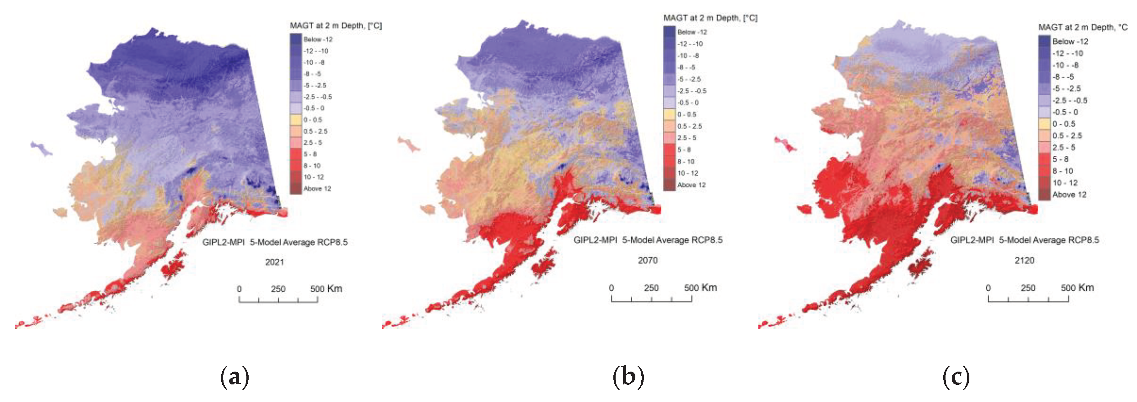
Figure C2.
The GIPL2-MPI modeled top of permafrost (permafrost table) position for 2021 (a), 2070 (b) and 2120 (c) snap shots using 5-Model Average composite RCP-4.5 as a climate forcing.
Figure C2.
The GIPL2-MPI modeled top of permafrost (permafrost table) position for 2021 (a), 2070 (b) and 2120 (c) snap shots using 5-Model Average composite RCP-4.5 as a climate forcing.
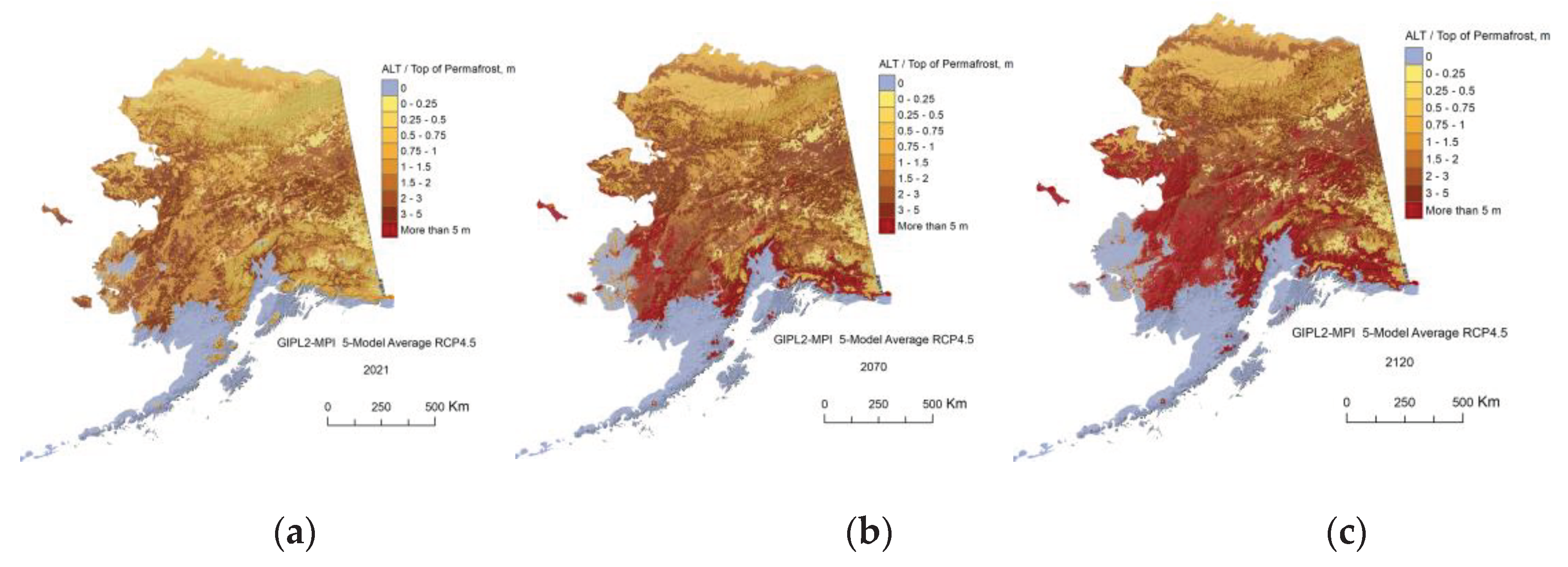
Figure C3.
The GIPL2-MPI modeled Talik thickness for 2021 (a), 2070 (b) and 2120 (c) snap shots using 5-Model Average composite RCP-4.5 as a climate forcing.
Figure C3.
The GIPL2-MPI modeled Talik thickness for 2021 (a), 2070 (b) and 2120 (c) snap shots using 5-Model Average composite RCP-4.5 as a climate forcing.
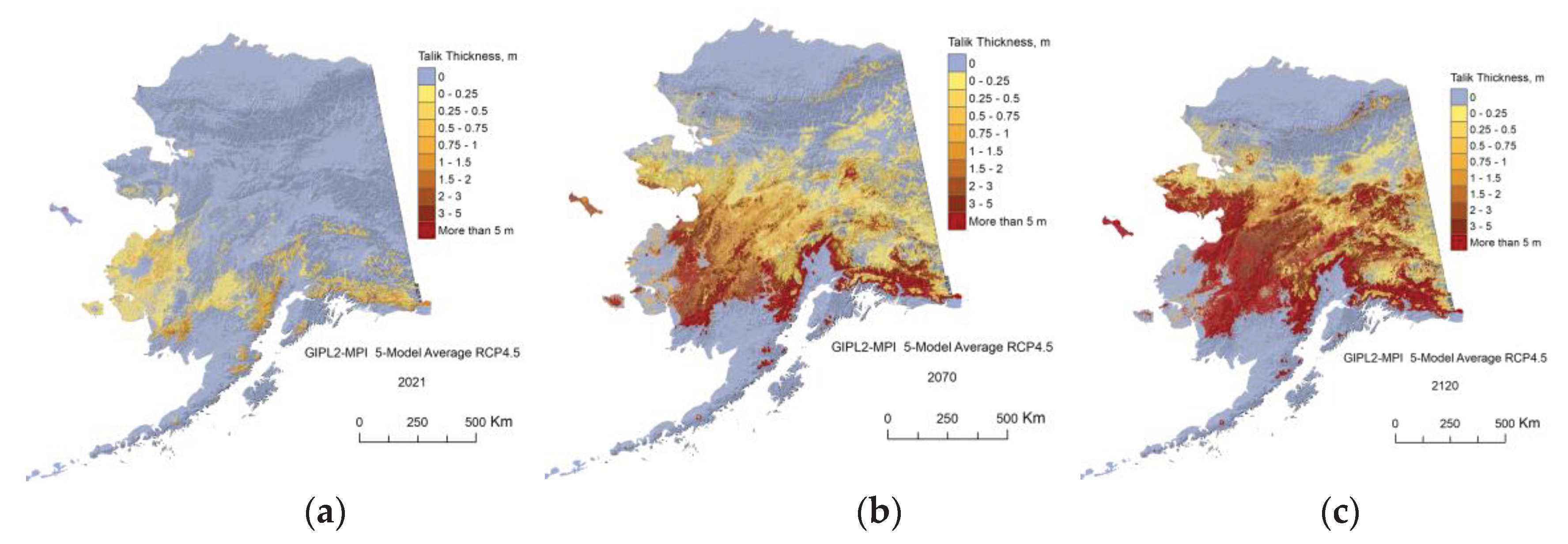
Figure C4.
The GIPL2-MPI modeled MAGT at 2 m depth for 2021 (a), 2070 (b) and 2120 (c) snap shots using 5-Model Average composite RCP-8.5 as a climate forcing.
Figure C4.
The GIPL2-MPI modeled MAGT at 2 m depth for 2021 (a), 2070 (b) and 2120 (c) snap shots using 5-Model Average composite RCP-8.5 as a climate forcing.
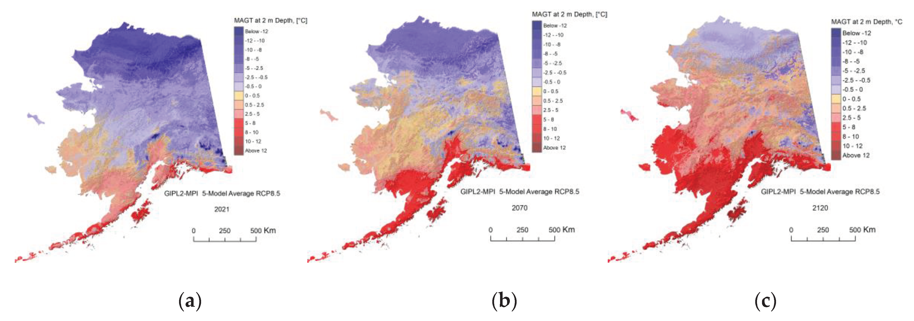
Figure C5.
The GIPL2-MPI modeled top of permafrost (permafrost table) position for 2021 (a), 2070 (b) and 2120 (c) snap shots using 5-Model Average composite RCP-8.5 as a climate forcing.
Figure C5.
The GIPL2-MPI modeled top of permafrost (permafrost table) position for 2021 (a), 2070 (b) and 2120 (c) snap shots using 5-Model Average composite RCP-8.5 as a climate forcing.
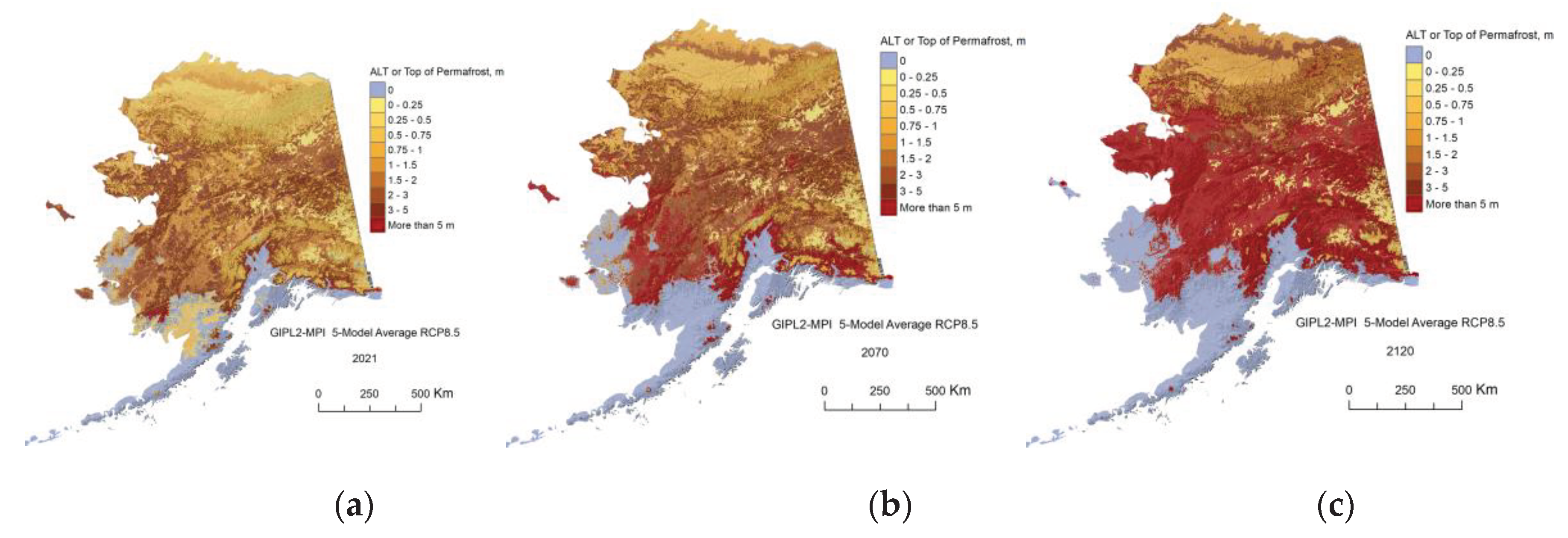
Figure C6.
The GIPL2-MPI modeled Talik thickness for 2021 (a), 2070 (b) and 2120 (c) snap shots using 5-Model Average composite RCP-8.5 as a climate forcing.
Figure C6.
The GIPL2-MPI modeled Talik thickness for 2021 (a), 2070 (b) and 2120 (c) snap shots using 5-Model Average composite RCP-8.5 as a climate forcing.
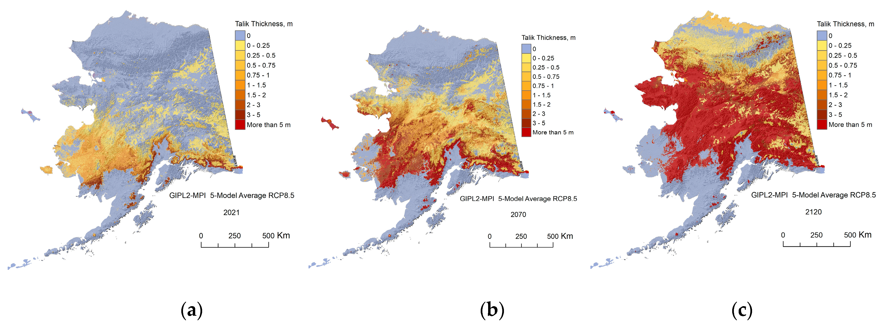
Figure C7.
The GIPL2-MPI modeled MAGT at 2 m depth for 2021 (a), 2070 (b) and 2120 (c) using GFDL-CM3 RCP-4.5 as a climate forcing.
Figure C7.
The GIPL2-MPI modeled MAGT at 2 m depth for 2021 (a), 2070 (b) and 2120 (c) using GFDL-CM3 RCP-4.5 as a climate forcing.
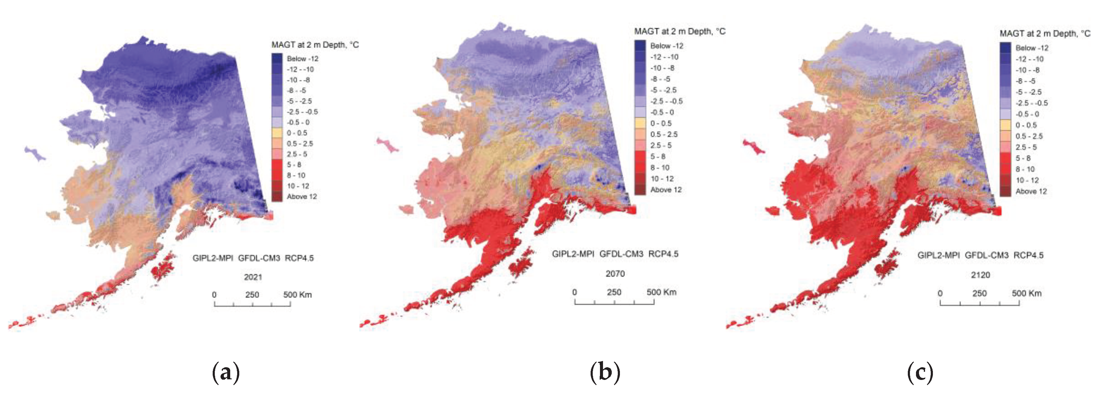
Figure C8.
The GIPL2-MPI modeled top of permafrost (permafrost table) position for 2021 (a), 2070 (b) and 2120 (c) using GFDL-CM3 RCP-4.5 as a climate forcing.
Figure C8.
The GIPL2-MPI modeled top of permafrost (permafrost table) position for 2021 (a), 2070 (b) and 2120 (c) using GFDL-CM3 RCP-4.5 as a climate forcing.
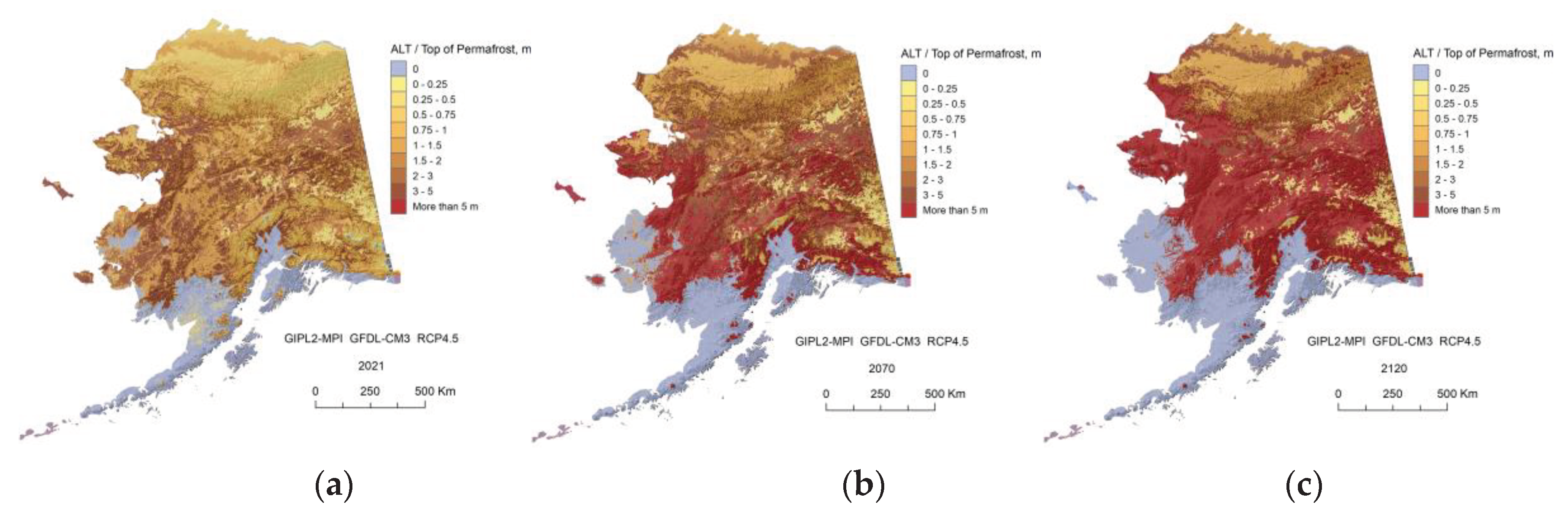
Figure C9.
The GIPL2-MPI modeled Talik thickness for 2021 (a), 2070 (b) and 2120 (c) using GFDL-CM3 RCP-4.5 as a climate forcing.
Figure C9.
The GIPL2-MPI modeled Talik thickness for 2021 (a), 2070 (b) and 2120 (c) using GFDL-CM3 RCP-4.5 as a climate forcing.
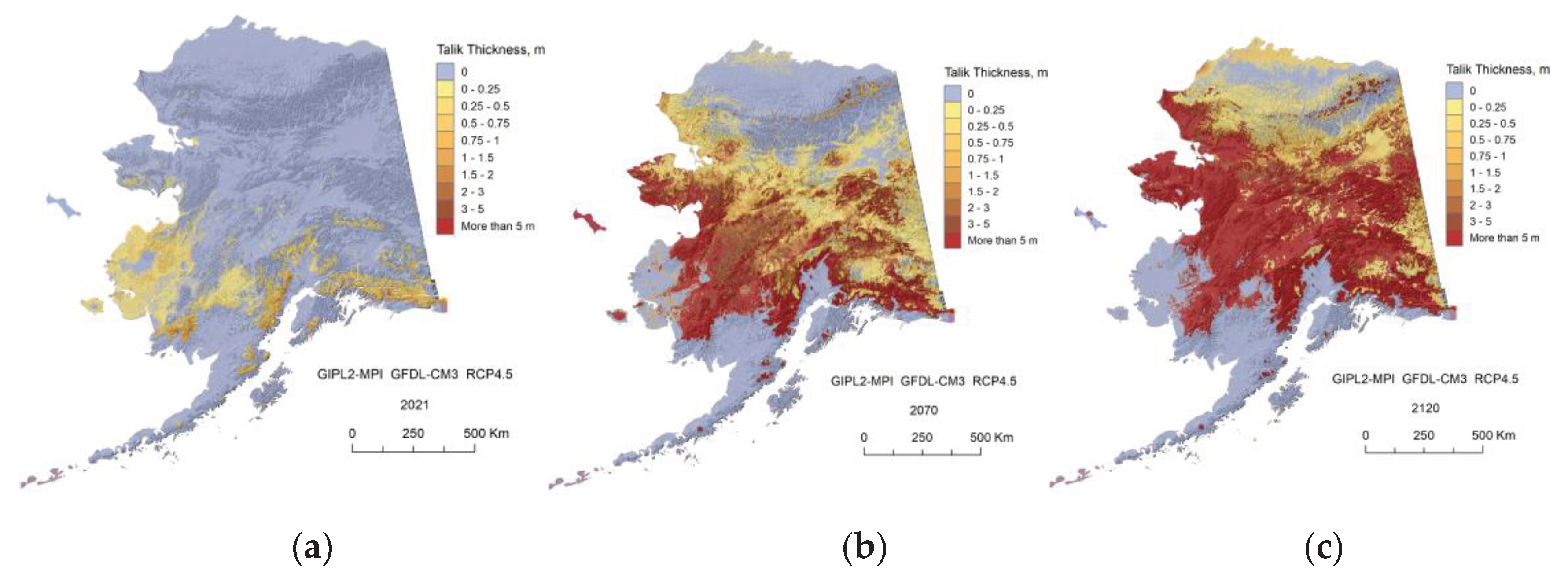
Figure C10.
The GIPL2-MPI modeled MAGT at 2 m depth for 2021 (a), 2070 (b) and 2120 (c) using GFDL-CM3-8.5 RCP-8.5 as a climate forcing.
Figure C10.
The GIPL2-MPI modeled MAGT at 2 m depth for 2021 (a), 2070 (b) and 2120 (c) using GFDL-CM3-8.5 RCP-8.5 as a climate forcing.
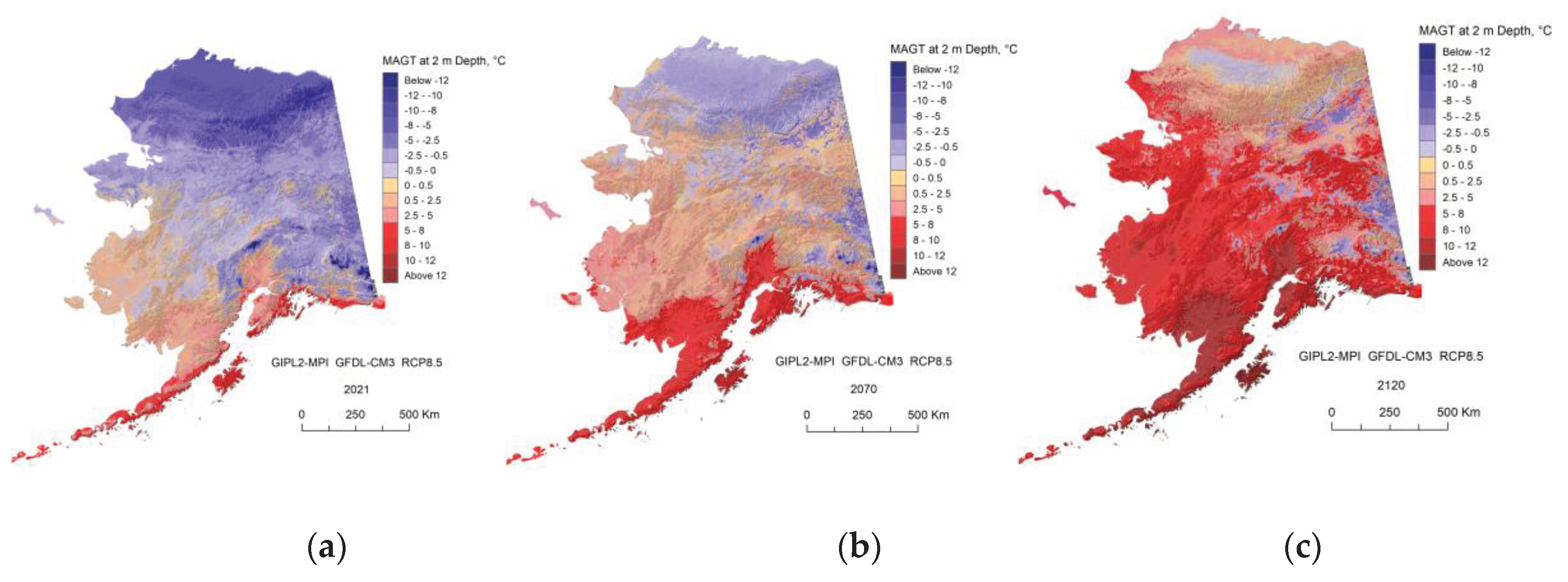
Figure C11.
The GIPL2-MPI modeled top of permafrost (permafrost table) position for 2021 (a), 2070 (b) and 2120 (c) using GFDL-CM3 RCP-8.5 as a climate forcing.
Figure C11.
The GIPL2-MPI modeled top of permafrost (permafrost table) position for 2021 (a), 2070 (b) and 2120 (c) using GFDL-CM3 RCP-8.5 as a climate forcing.
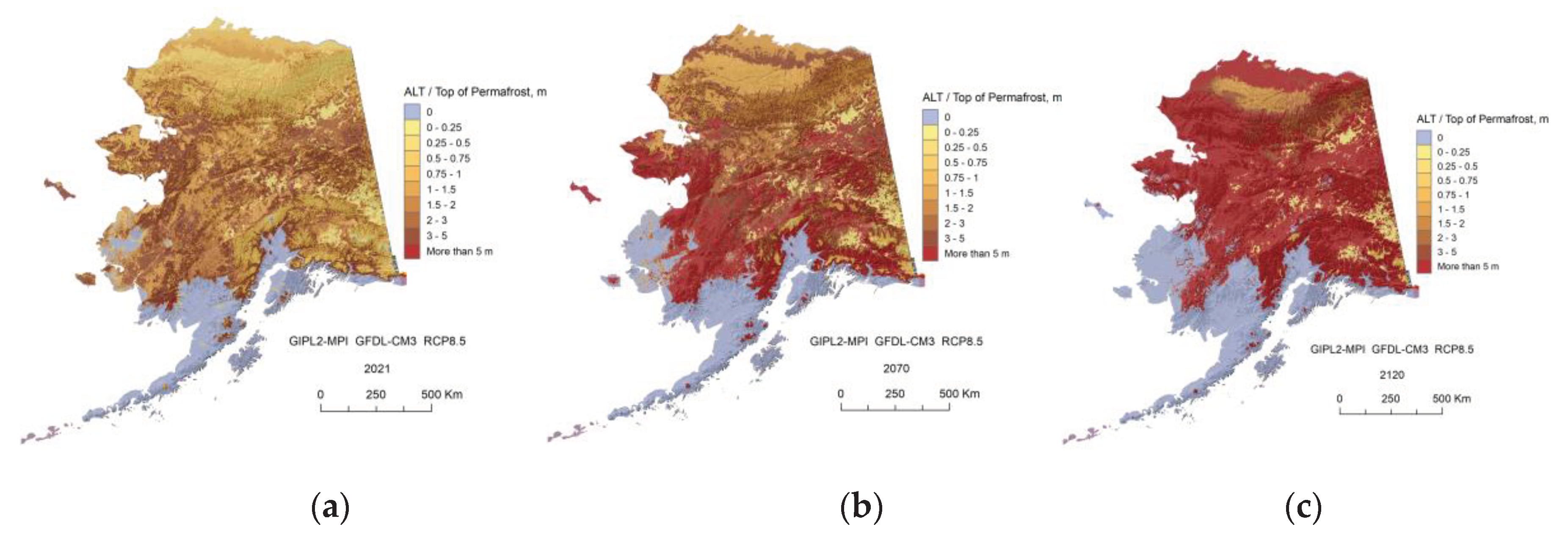
Figure C12.
The GIPL2-MPI modeled Talik thickness for 2021 (a), 2070 (b) and 2120 (c) using GFDL-CM3 RCP-8.5 as a climate forcing.
Figure C12.
The GIPL2-MPI modeled Talik thickness for 2021 (a), 2070 (b) and 2120 (c) using GFDL-CM3 RCP-8.5 as a climate forcing.
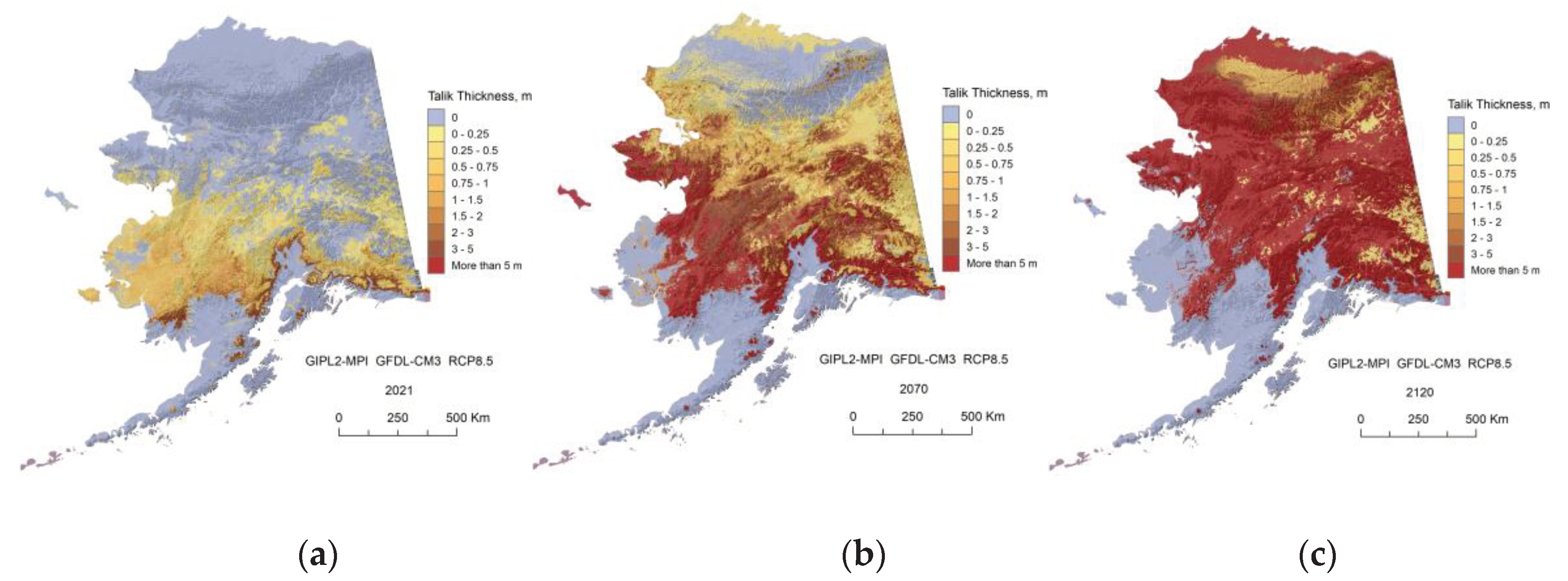
Figure C13.
The GIPL2-MPI modeled MAGT at 2 m depth for 2021 (a), 2070 (b) and 2120 (c) using NCAR-CCSM4 RCP-4.5 as a climate forcing.
Figure C13.
The GIPL2-MPI modeled MAGT at 2 m depth for 2021 (a), 2070 (b) and 2120 (c) using NCAR-CCSM4 RCP-4.5 as a climate forcing.
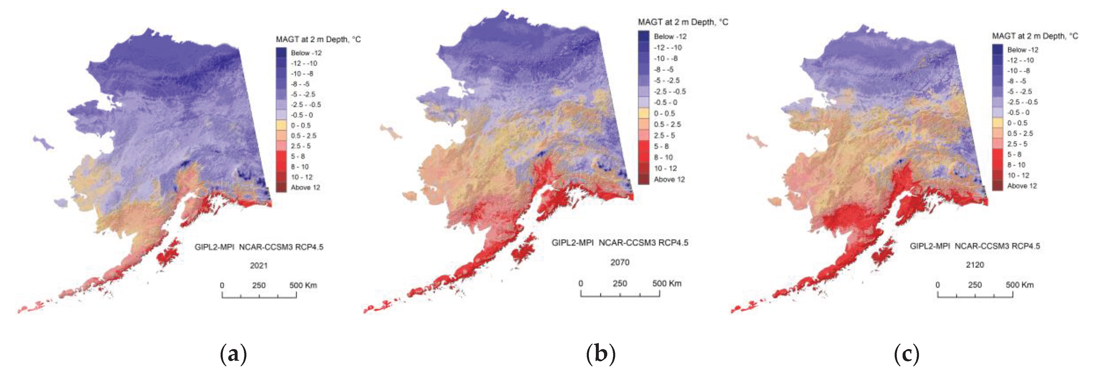
Figure C14.
The GIPL2-MPI modeled top of permafrost (permafrost table) position for 2021 (a), 2070 (b) and 2120 (c) using NCAR-CCSM4 RCP-4.5 as a climate forcing.
Figure C14.
The GIPL2-MPI modeled top of permafrost (permafrost table) position for 2021 (a), 2070 (b) and 2120 (c) using NCAR-CCSM4 RCP-4.5 as a climate forcing.
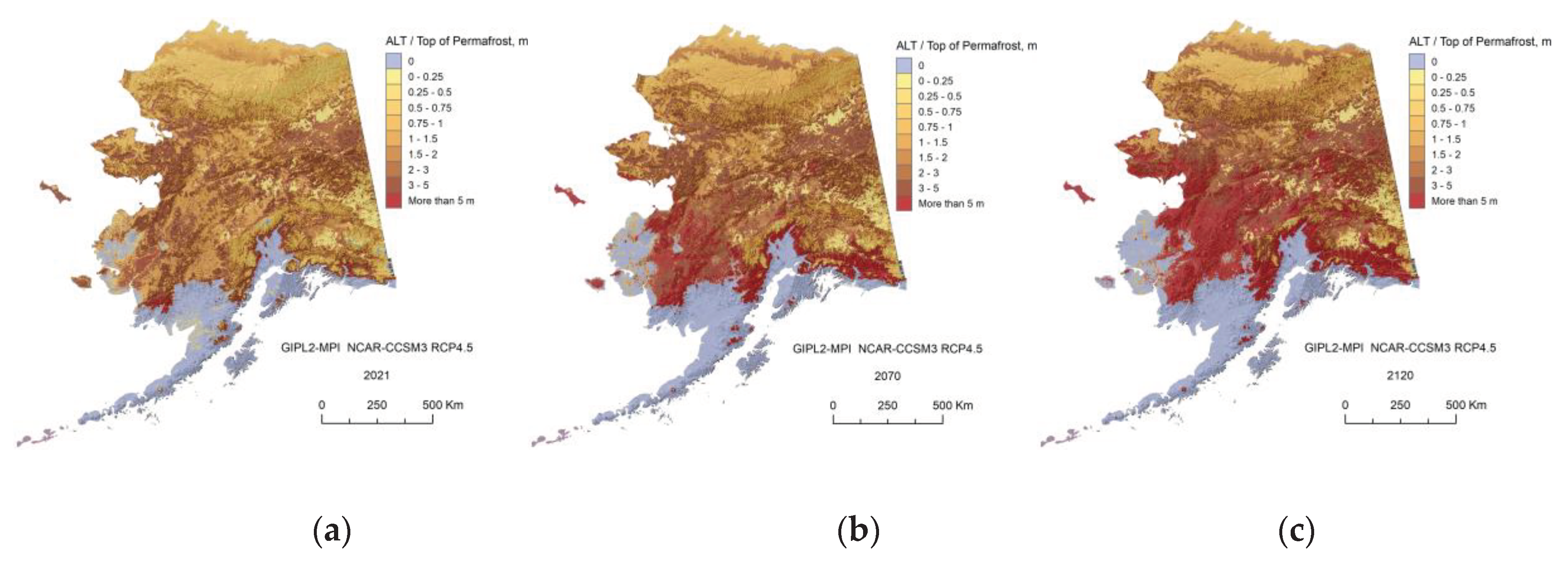
Figure C15.
The GIPL2-MPI modeled Talik thickness for 2021 (a), 2070 (b) and 2120 (c) using NCAR-CCSM4 RCP-4.5 as a climate forcing.
Figure C15.
The GIPL2-MPI modeled Talik thickness for 2021 (a), 2070 (b) and 2120 (c) using NCAR-CCSM4 RCP-4.5 as a climate forcing.
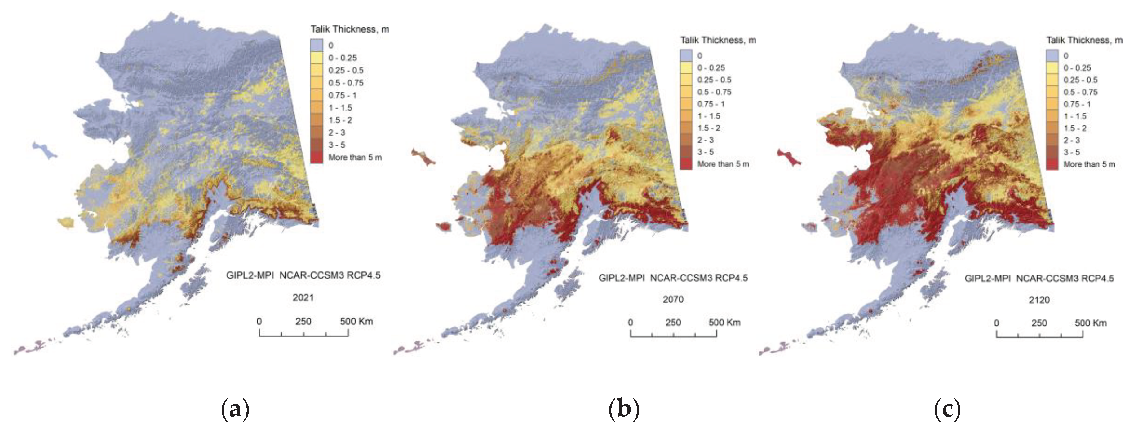
Figure C16.
The GIPL2 modeled MAGT temperature at 2 m depth for 2021 (a), 2070 (b) and 2120 (c) using NCAR-CCSM4 8.5 Representative Concentration Pathway (RCP 8.5) as a climate forcing.
Figure C16.
The GIPL2 modeled MAGT temperature at 2 m depth for 2021 (a), 2070 (b) and 2120 (c) using NCAR-CCSM4 8.5 Representative Concentration Pathway (RCP 8.5) as a climate forcing.
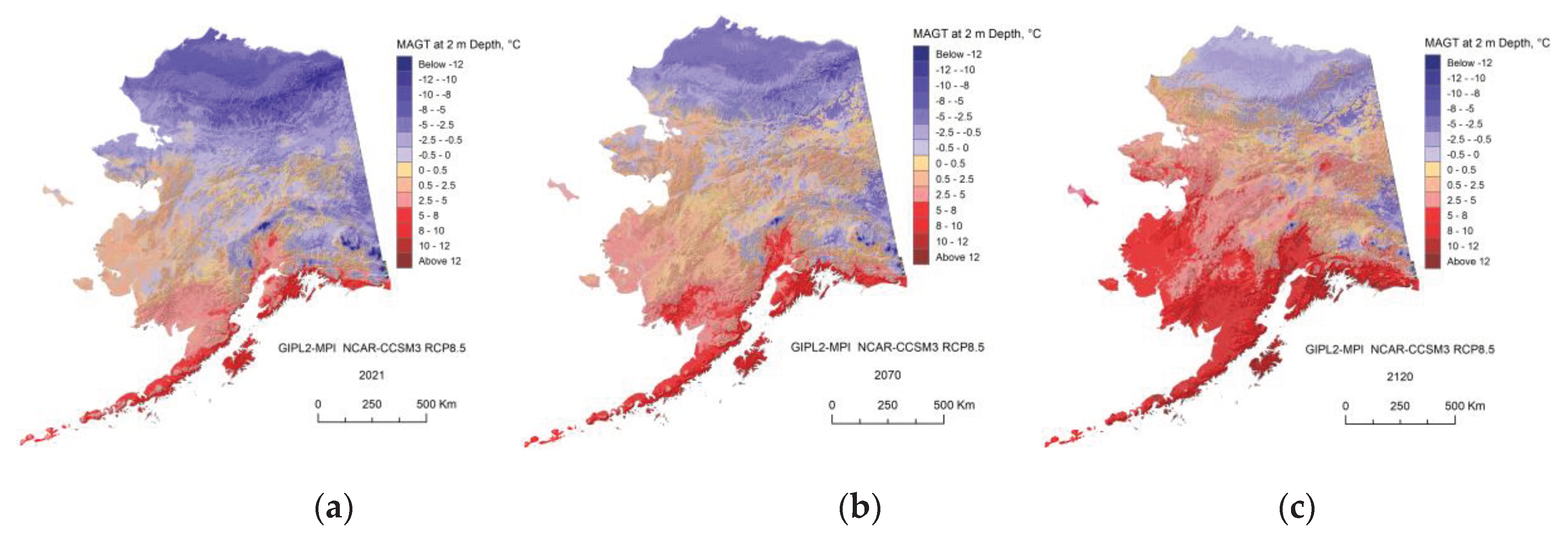
Figure C17.
The GIPL2 modeled top of permafrost (permafrost table) position for 2021 (a), 2070 (b) and 2120 (c) using NCAR-CCSM RCP-8.5 as a climate forcing.
Figure C17.
The GIPL2 modeled top of permafrost (permafrost table) position for 2021 (a), 2070 (b) and 2120 (c) using NCAR-CCSM RCP-8.5 as a climate forcing.
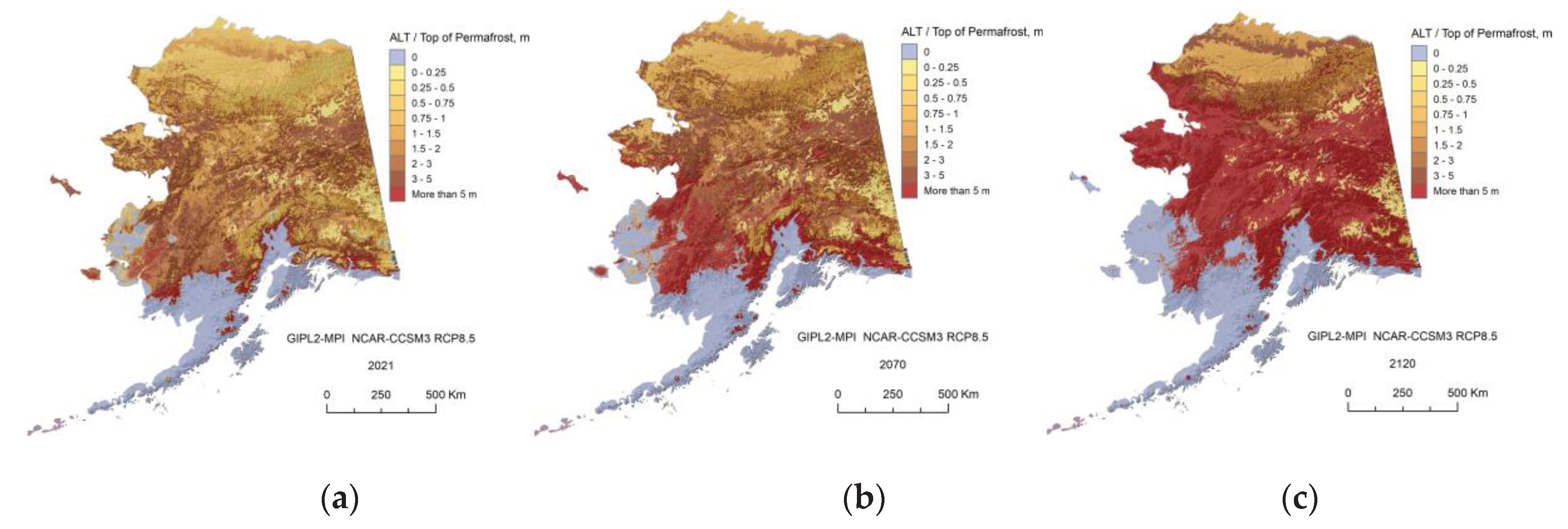
Figure C18.
The GIPL2 modeled Talik thickness for 2021 (a), 2070 (b) and 2120 (c) using NCAR-CCSM4 RCP-8.5 as a climate forcing.
Figure C18.
The GIPL2 modeled Talik thickness for 2021 (a), 2070 (b) and 2120 (c) using NCAR-CCSM4 RCP-8.5 as a climate forcing.
References
- Biskaborn, B.K.; Smith, S.L.; Noetzli, J.; Matthes, H.; Vieira, G.; Streletskiy, D.A.; Schoeneich, P.; Romanovsky, V.E.; Lewkowicz, A.G.; Abramov, A.; Allard, M. Permafrost is warming at a global scale. Nat. Commun. 2019, 10, 264. [Google Scholar] [CrossRef]
- Romanovsky, V.; Marchenko, S.S.; Kholodov, A.L.; Oberman, N.G.; Drozdov, D.S.; Malkova, G.V.; Vasiliev, A.A.; Sergeev, D.O.; Zheleznyak, M.N. Thermal State and Fate of Permafrost in Russia: First Results of IPY (Plenary Paper). In: Proc 9th Int Conf on Permafrost (Kane DL & Hinkel KM, Eds), Univ AK Fairbanks, June 29 - July 3, 2008, Vol. II: 1511-1518.
- Romanovsky, V.E.; Smith, S.L.; Christiansen, H.H. Permafrost thermal state in the polar northern hemisphere during the International Polar Year 2007-2009: a synthesis. Permafrost and Periglacial Processes 2010, 21, 106–116. [Google Scholar] [CrossRef]
- Smith, S.L.; Romanovsky, V.E.; Lewkowicz, A.G.; Burn, C.R.; Allard, M.; Clow, G.D.; Yoshikawa, K.; Thoop, J. . Thermal state of permafrost in North America - A contribution to the International Polar Year. Permafrost and Periglacial Processes 2010, 21, 117–135. [Google Scholar] [CrossRef]
- Osterkamp, T.E. Establishing long-term permafrost observatories for active layer and permafrost investigations in Alaska: 1977–2002. Permafrost Periglacial Processes 2003, 14, 331–342. [Google Scholar] [CrossRef]
- Osterkamp, T.E. The Recent Warming of Permafrost in Alaska. Global Planet Change 2005, 49, 187–202. [Google Scholar] [CrossRef]
- Osterkamp, T.E.; Gosink, J.P.; Kawasaki, K. Measurements of permafrost temperatures to evaluate the consequences of recent climate warming; final report, Contract 84 NX 203 F 233181; Alaska Dept. of Transp. Public Facil.: Fairbanks, Alaska, 1987. [Google Scholar]
- Osterkamp, T.E.; Gosink, J.P.; Kawasaki, K. Permafrost temperature measurements in an Alaskan transect: Preliminary results; Spec. Rep. 1984, 85-5; U.S. Army Cold Reg. Res. and Eng. Lab.: Hanover, NH.
- Osterkamp, T.E. Thermal state of permafrost in Alaska during the fourth quarter of the twentieth century. In Proceedings of the Ninth International Conference on Permafrost, Fairbanks, Alaska, 29 June–3 July 2008; Volume 2, pp. 1333–1338. [Google Scholar]
- ACIA. Arctic Climate Impact Assessment. ACIA Overview report. 2005. Cambridge University Press. 1020pp.
- Boer, G.J.; Flato, G.M.; Reader, M.C.; Ramsden, D. A transient climate change simulation with historical and projected greenhouse gas and aerosol forcing: experimental design and comparison with the instrumental record for the 20th century. Climate Dynamics 2000, 16, 405–425. [Google Scholar] [CrossRef]
- IPCC, 2013: Climate Change 2013: The Physical Science Basis. Contribution of Working Group I to the Fifth Assessment Report of the Intergovernmental Panel on Climate Change [Stocker, T.F., D. Qin, G.-K. Plattner, M. Tignor, S.K. Allen, J. Boschung, A. Nauels, Y. Xia, V. Bex and P.M. Midgley (eds.)]. Cambridge University Press, Cambridge, United Kingdom and New York, NY, USA, 1535 pp.
- IPCC, 2014: Climate Change 2014: Synthesis Report. Contribution of Working Groups I, II and III to the Fifth Assessment Report of the Intergovernmental Panel on Climate Change [Core Writing Team, R.K. Pachauri and L.A. Meyer (eds.)]. IPCC, Geneva, Switzerland, 151 pp.
- IPCC, 2022: Climate Change 2022: Mitigation of Climate Change. Contribution of Working Group III to the Sixth Assessment Report of the Intergovernmental Panel on Climate Change [P.R. Shukla, J. Skea, R. Slade, A. Al Khourdajie, R. van Diemen, D. McCollum, M. Pathak, S. Some, P. Vyas, R. Fradera, M. Belkacemi, A. Hasija, G. Lisboa, S. Luz, J. Malley, (eds.)]. Cambridge University Press, Cambridge, UK and New York, NY, USA. [CrossRef]
- Jorgenson, M.T.; Racine, C.H.; Walters, J.C.; Osterkamp, T.E. . Permafrost degradation and ecological changes associated with a warming climate in central Alaska. Climatic Change 2001, 48, 551–571. [Google Scholar] [CrossRef]
- Racine, C.H.; Walters, J.C. Groundwater-discharge fens in the Tanana Lowlands, Interior Alaska, U.S.A. Arctic and Alpine Research 1994, 26, 418–426. [Google Scholar] [CrossRef]
- Osterkamp, T.E.; Jorgenson, J.C. Warming of Permafrost in the Arctic National Wildlife Refuge, Alaska. Permafrost and Periglacial Process 2006, 17, 65–69. [Google Scholar] [CrossRef]
- Shur, Y.L.; Jorgenson, M.T. Patterns of permafrost formation and degradation in relation to climate and ecosystems. Permafr Periglac Process 2007, 18, 7–19. [Google Scholar] [CrossRef]
- Jorgenson, M.T.; Shur, Y.L.; Osterkamp, T.E. Thermokarst in Alaska (Plenary Paper). In Proceedings of the Ninth International Conference on Permafrost, Fairbanks, Alaska, 29 June–3 July 2008; Vol. II; pp. 869–876. [Google Scholar]
- Chapman, W.L.; Walsh, J.E. Simulations of Arctic temperature and pressure by global coupled models. J. Climate 2007, 20, 609–632. [Google Scholar] [CrossRef]
- Marchenko, S.S.; Romanovsky, V.E.; Tipenko, G.S. Numerical Modeling of Spatial Permafrost Dynamics in Alaska. In Proceedings of the Ninth International Conference on Permafrost (D. Kane and K. Hinkel Eds), University of Alaska Fairbanks, 29 Jun–3 July 2008; 2: 1125-1130.
- Sergey Marchenko. Arctic and Subarctic Engineering Design Tool: Technology Transfer UFC 3-130 (Year 1 Contract Report W913E521C0010). The U.S. Army Engineer Research and Development Center (ERDC), Cold Regions Research and Engineering Laboratory (CRREL), November 2022, Hanover, NH, 03755 https://drive.google.com/file/d/1UBnb7uqM6bEkppAeaYkq9bJdDHymTMae/view.
- Marchenko, S.S. A Model of Permafrost Formation and Occurrences in the Intracontinental Mountains. Norsk Geografisk Tidsskrift 2001, 55, 230–234. [Google Scholar] [CrossRef]
- Nicolsky, D.J.; Romanovsky, V.E.; Panda, S.K.; Marchenko, S.S.; Muskett, R.R. . Applicability of the ecosystem type approach to model permafrost dynamics across the Alaska North Slope. J. Geophys. Res. Earth Surf. 2017, 121. [Google Scholar] [CrossRef]
- Jafarov, E.E.; Marchenko, S.S.; Romanovsky, V.E. . Numerical Modeling of Permafrost Dynamics in Alaska Using a High Spatial Resolution Dataset. The Cryosphere 2012, 6, 613–624. [Google Scholar] [CrossRef]
- Westermann, S.; Schuler, T.; Gisnås, K.; Etzelmüller, B. . Transient thermal modeling of permafrost conditions in southern Norway. Cryosphere 2013, 7, 719–739. [Google Scholar] [CrossRef]
- Westermann, S.; Langer, M.; Boike, J.; Heikenfeld, M.; Peter, M.; Etzelmüller, B.; Krinner, G. . Simulating the thermal regime and thaw processes of ice-rich permafrost ground with the land-surface model CryoGrid 3. Geosci. Model Dev. 2016, 9, 523–546. [Google Scholar] [CrossRef]
- Zhang, Y.; Wang, X.; Fraser, R.; Olthof, I.; Chen, W.; Mclennan, D.; Ponomarenko, S.; Wu, W. Modelling and mapping climate change impacts on permafrost at high spatial resolution for an Arctic region with complex terrain. Cryosphere 2013, 7, 1121–1137. [Google Scholar] [CrossRef]
- Fiddes, J.; Endrizzi, S.; Gruber, S. Large-area land surface simulations in heterogeneous terrain driven by global data sets: Application to mountain permafrost. Cryosphere 2015, 9, 411–426. [Google Scholar] [CrossRef]
- Rawlins, M.A.; Nicolsky, D.J.; McDonald, K.C.; Romanovsky, V.E. Simulating soil freeze/thaw dynamics with an improved pan-Arctic water balance model. Journal of Advances in Modeling Earth Systems 2013, 5, 659–675. [Google Scholar] [CrossRef]
- Gisnas, K.; Westermann, S.; Schuler, T.V.; Melvold, K.; Etzelmuller, B. Small-scale variation of snow in a regional permafrost model. Cryosphere 2016, 10, 1201–1215. [Google Scholar] [CrossRef]
- Moss, R.; et al. Towards New Scenarios for Analysis of Emissions, Climate Change, Impacts and Response Strategies; Technical Summary; Intergovernmental Panel on Climate Change: Geneva, 2008. [Google Scholar]
- van Vuuren, D.P.; Edmonds, J.; Kainuma, M.; et al. The representative concentration pathways: an overview. Climatic Change 2011, 109, 5. [Google Scholar] [CrossRef]
- van Vuuren, D.P.; Eickhout, B.; Lucas, P.L.; den Elzen, M.G.J. Long-term multi-gas scenarios to stabilize radiative forcing — Exploring costs and benefits within an integrated assessment framework. Multigas mitigation and climate policy. Energy J. 2006, 3, 201–234. [Google Scholar] [CrossRef]
- Walsh, J.E.; Bhatt, U.S.; Littell, J.S.; Leonawicz, M.; Lindgren, M.; Kurkowski, T.A.; Bieniek, P.A.; Thoman, R.; Gray, S.; Rupp, T.S. Downscaling of climate model output for Alaskan stakeholders. Environmental Modelling & Software 2018, 110, 38–51. [Google Scholar] [CrossRef]
- Jorgenson, T.; Yoshikawa, K.; Kanevskiy, M.; Shur, Y.; Romanovsky, V.; Marchenko, S.; Grosse, G.; Brown, J.; Jones, B. Permafrost Characteristics of Alaska. In Proceedings of the Ninth International Conference on Permafrost (D. Kane and K. Hinkel Eds), University of Alaska Fairbanks, 29 June–3 July 2008; Extended Abstracts, 121-122.
- Nicolsky, D.; Romanovsky, V.; Panteleev, G. Estimation of soil thermal properties using in-situ temperature measurements in the active layer and permafrost. Cold Regions Science and Technology 2009, 55, 120–129. [Google Scholar] [CrossRef]
- Marchuk, G.I. Methods of Numerical Mathematics (Applications of Mathematics); Springer-Verlag: New York, 1975; 316p. [Google Scholar]
- Alexiades, V.; Solomon, A.D. Mathematical modeling of melting and freezing processes, Washington, Hemisphere, 1993, 325 pp.
- Verdi, C. Numerical aspects of parabolic free boundary and hysteresis problems; Lecture Notes in Mathematics; Springer-Verlag: New York, 1994; pp. 213–284. [Google Scholar]
- Pollack, H.N.; Hurter, S.J.; Johnson, J.R. Heat flow from the Earth's interior: analysis of the global data set. Reviews of Geophysics 1993, 31, 267–280. [Google Scholar] [CrossRef]
- He, Y.; Genet, H.; McGuire, A.D.; Zhuang, Q.; Wylie, B.K.; Zhang, Y. He, Y.; Genet, H.; McGuire, A.D.; Zhuang, Q.; Wylie, B.K.; Zhang, Y. Terrestrial carbon modeling - Baseline and projections in lowland ecosystems of Alaska, chap. 7 in Zhu, Z., and McGuire, A.D., eds., Baseline and projected future carbon storage and greenhouse-gas fluxes in ecosystems of Alaska: U. S. Geological Survey Professional Paper. 2016, 1826, p. 133-158. [CrossRef]
- McGuire, A.D. McGuire, A.D., Genet, H., He, Y., Stackpoole, S., D'Amore, D.V., Rupp, T.S., Wylie, B.K., Zhou, X., and Zhu, Z. Alaska carbon balance, chap. 9 in Zhu, Z., and McGuire, A.D., eds., Baseline and projected future carbon storage and green-house-gas fluxes in ecosystems of Alaska: U. S. Geological Survey Professional Paper 1826, 2016, p. 189-196. [CrossRef]
- Baseline and projected future carbon storage and greenhouse-gas fluxes in ecosystems of Alaska: U.S. Geological Survey Professional Paper. (Zhu, Z., and McGuire, A.D. eds.), 2016, 1826, 196 p. [CrossRef]
- Geological Survey, U.S, and Arch C Gerlach. The national atlas of the United States of America. Washington, 1985. Map.
- The 2010 Land Cover of North America at 30 meters, Edition: 1.0, U.S. Geological Survey (USGS), Land Cover Map. http://www.cec.org/tools-and-resources/map-files/land-cover-2010-landsat-30m.
- Shangguan, W.; Hengl, T.; Mendes de Jesus, J.; Yuan, H.; Dai, Y. Mapping the global depth to bedrock for land surface modeling. J. Adv. Model. Earth Syst. 2017, 9, 65–88. [Google Scholar] [CrossRef]
- Kreig, R.A.; Reger, R.D. Air-photo analysis and summary of landform soil properties along the route of the Trans-Alaska Pipeline System. Alaska Div. Geol. Geophys. Surv., Geologic Rep. 1982, 66, 149. [Google Scholar]
- Romanovsky, V.E.; Osterkamp, T.E. Effects of unfrozen water on heat and mass transport processes in the active layer and permafrost. Permafrost and Periglacial Processes 2000, 11, 219–239. [Google Scholar] [CrossRef]
- Nicolsky, D.; Romanovsky, V.; Tipenko, G. . Estimation of thermal properties of saturated soils using in-situ temperature measurements. Cryosphere 2007, 1, 41–58. [Google Scholar] [CrossRef]
- Huang, F.; Zhan, F.; Ju, W.; Wang, Z. Improved reconstruction of soil thermal field using two-depth measurements of soil temperature. Journal of Hydrology 2014, 519, 711–719. [Google Scholar] [CrossRef]
- Hirota, T.; Pomeroy, J.W.; Granger, R.J.; Maule, C.P. An extension of the force-restore method to estimate soil temperature at depth and evaluation for frozen soils under snow. J. Geophys. Res. 2002, 107, 4767. [Google Scholar] [CrossRef]
- Multi-Language Glossary of Permafrost and Related Ground-Ice Terms; van Everdingen, R.O., Ed.; University of Calgary: Calgary, 1998. [Google Scholar]
- Harris, S.A.; French, H.M.; Heginbottom, J.A.; Johnston, G.H.; Ladanyi, B.; Sego, D.C.; van Everdingen, R.O. National Research Council of Canada. Ottawa, Ontario, Canada KIA OR6. Technical Memorandum. 1998. No. 142.
- NSIDC Cryosphere glossary 2023. National Snow and Ice Data Center - Advancing knowledge of Earth's frozen regions. https://nsidc.org/learn/cryosphere-glossary.
- A Dictionary of Geology and Earth Sciences (5 ed). Michael Allaby. (2020) Oxford Uni-versity Press. Print ISBN-13: 9780198839033. Published online: 2020. Current Online Version: 2020, eISBN: 9780191874901. [CrossRef]
- Sturm, M.; Holmgren, J.; König, M.; Morris, K. The thermal conductivity of seasonal snow. Journal of Glaciology 1997, 43, 26–41. [Google Scholar] [CrossRef]
- Yershov, E. General Geocryology; Cambridge Univ. Press: Cambridge, 1998; 580p. [Google Scholar]
- US Army Corps of Engineers 1954. Report on foundation investigations, Project F-23. Gulkana, Alaska.
- Ferrians, O.J. 1971. Preliminary engineering geologic maps of the proposed Trans-Alaska pipeline route, Gulkana Quadrangle: US Geological Survey Open File Report 71–102, 2 sheets, scale 1:125.000.
- CRREL 1964. Ground temperature observations Gulkana, Alaska. USA CRREL Technical Report 106.
Figure 1.
Exceptionally ice-rich permafrost with ground ice in a close proximity to the ground surface: (a) Itkilik River on North Slope Alaska (photo courtesy M. Kanevskyi); (b) Interior Alaska, Fairbanks vicinity (photo courtesy I. Semiletov).
Figure 1.
Exceptionally ice-rich permafrost with ground ice in a close proximity to the ground surface: (a) Itkilik River on North Slope Alaska (photo courtesy M. Kanevskyi); (b) Interior Alaska, Fairbanks vicinity (photo courtesy I. Semiletov).
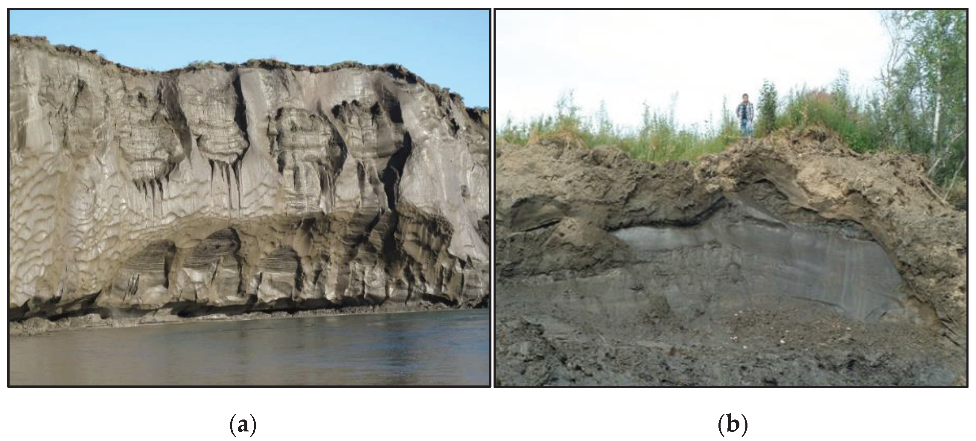
Figure 2.
(a) Alaska Region Digital Elevation Model (ARDEM) v2.0 with nominal 1-km grid spacing over the domain 51°N-71°N and 179°W-117°W, which is represent the computational domain across entire Alaska; (b) permafrost distribution [36] and permafrost observing site locations across Alaska.
Figure 2.
(a) Alaska Region Digital Elevation Model (ARDEM) v2.0 with nominal 1-km grid spacing over the domain 51°N-71°N and 179°W-117°W, which is represent the computational domain across entire Alaska; (b) permafrost distribution [36] and permafrost observing site locations across Alaska.
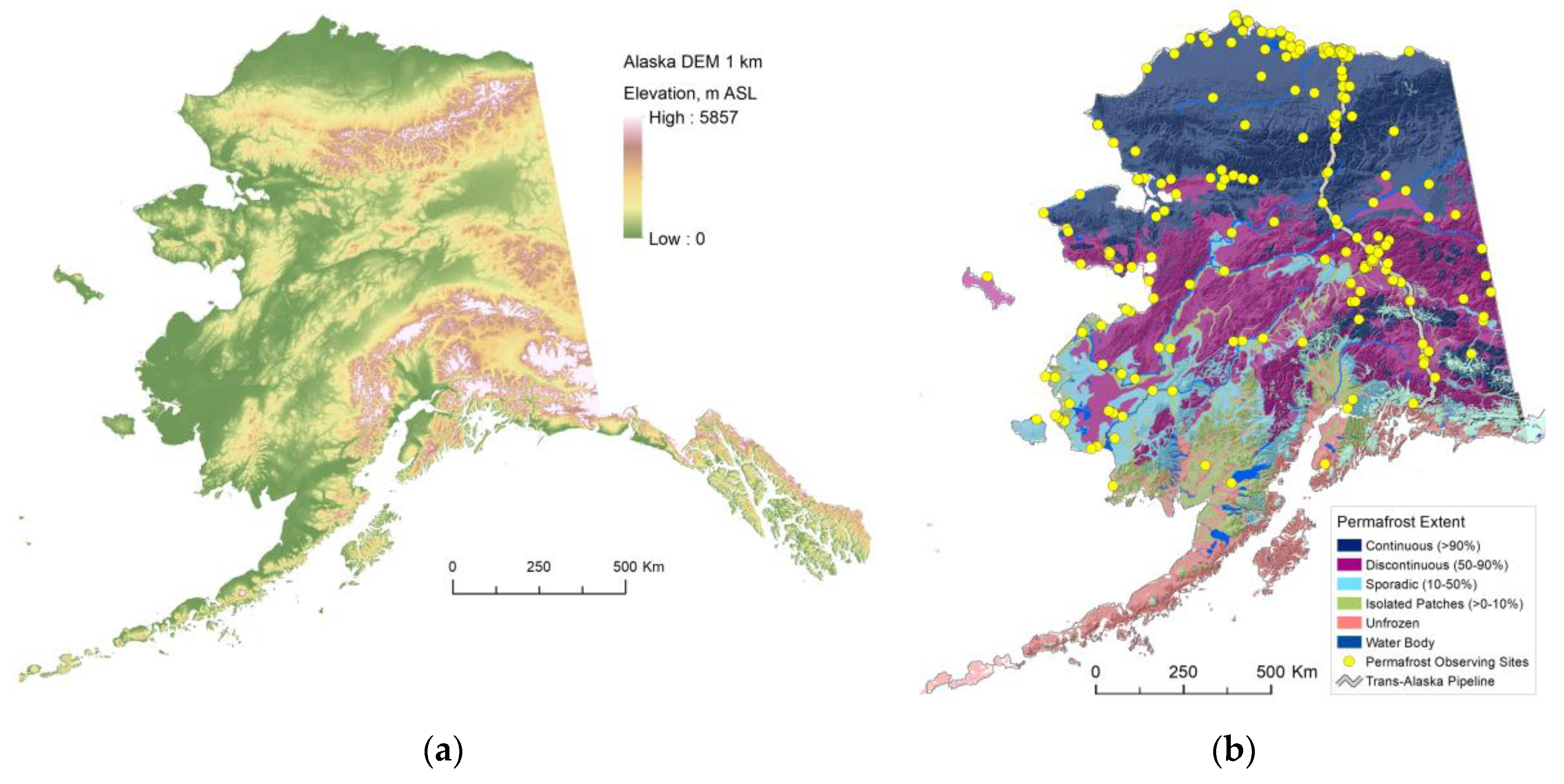
Figure 3.
Global mean temperature change averaged across all Coupled Model Intercomparison Project Phase 5 (CMIP5) models (relative to 1986–2005) for the four Representative Concentration Pathway (RCP) scenarios: RCP2.6 (dark blue), RCP4.5 (light blue), RCP6.0 (orange) and RCP8.5 (red). Likely ranges for global temperature change by the end of the 21st century are indicated by vertical bars. After [12].
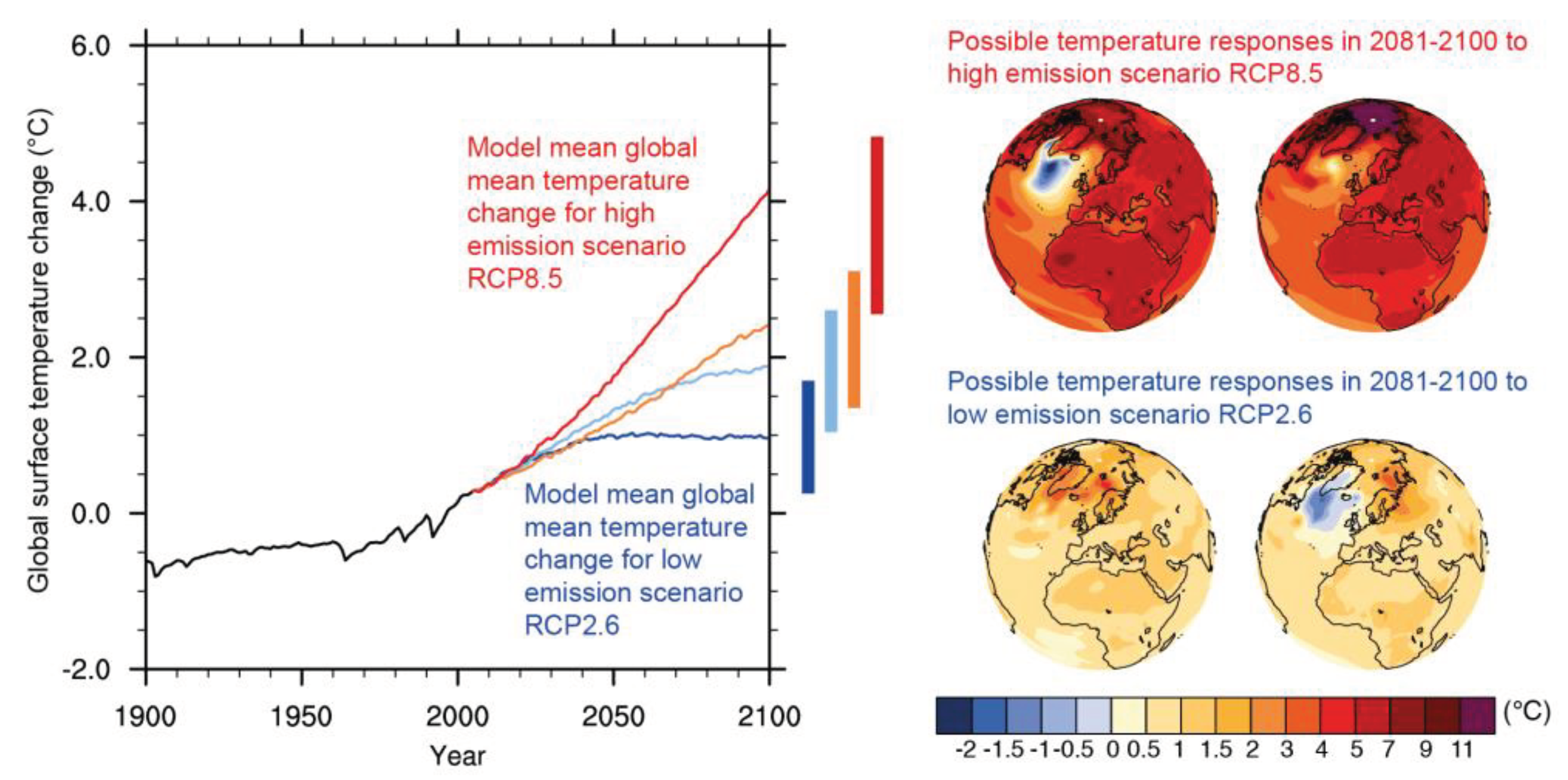
Figure 4.
Major Ecosystems of Alaska [44] (a) and Alaska Wetland Composite Map at 30 m spatial resolution (b) [42,43] used for prescription of initial soil moisture and soil thermal properties of the upper layers of soil column and surface vegetation.
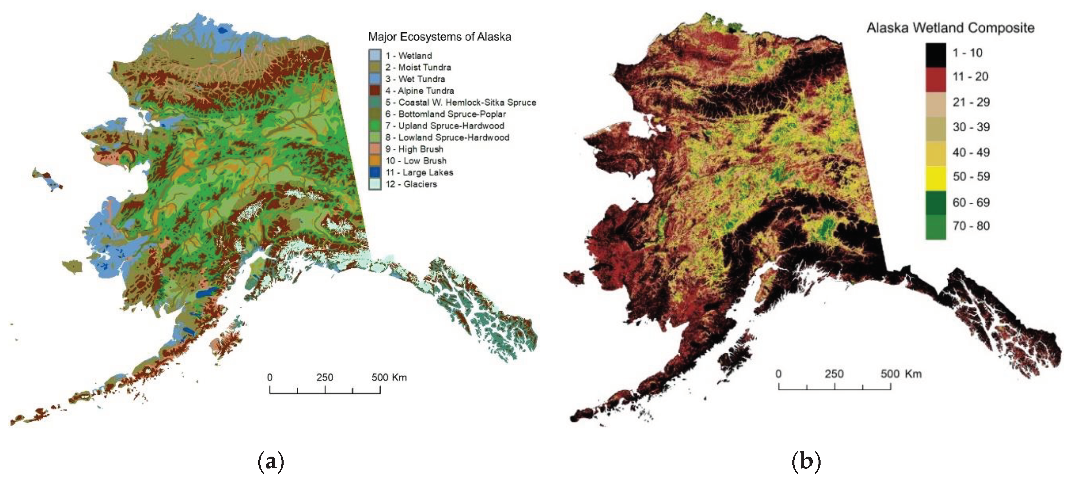
Figure 5.
Statewide Vegetation/Land Cover (AVHRR/NDVI) Map (a) was used for initially prescribed surface vegetation and upper soil properties [46]. Map of Deposit Type of Alaska [36] used for determination of initial properties of deeper layers (b).
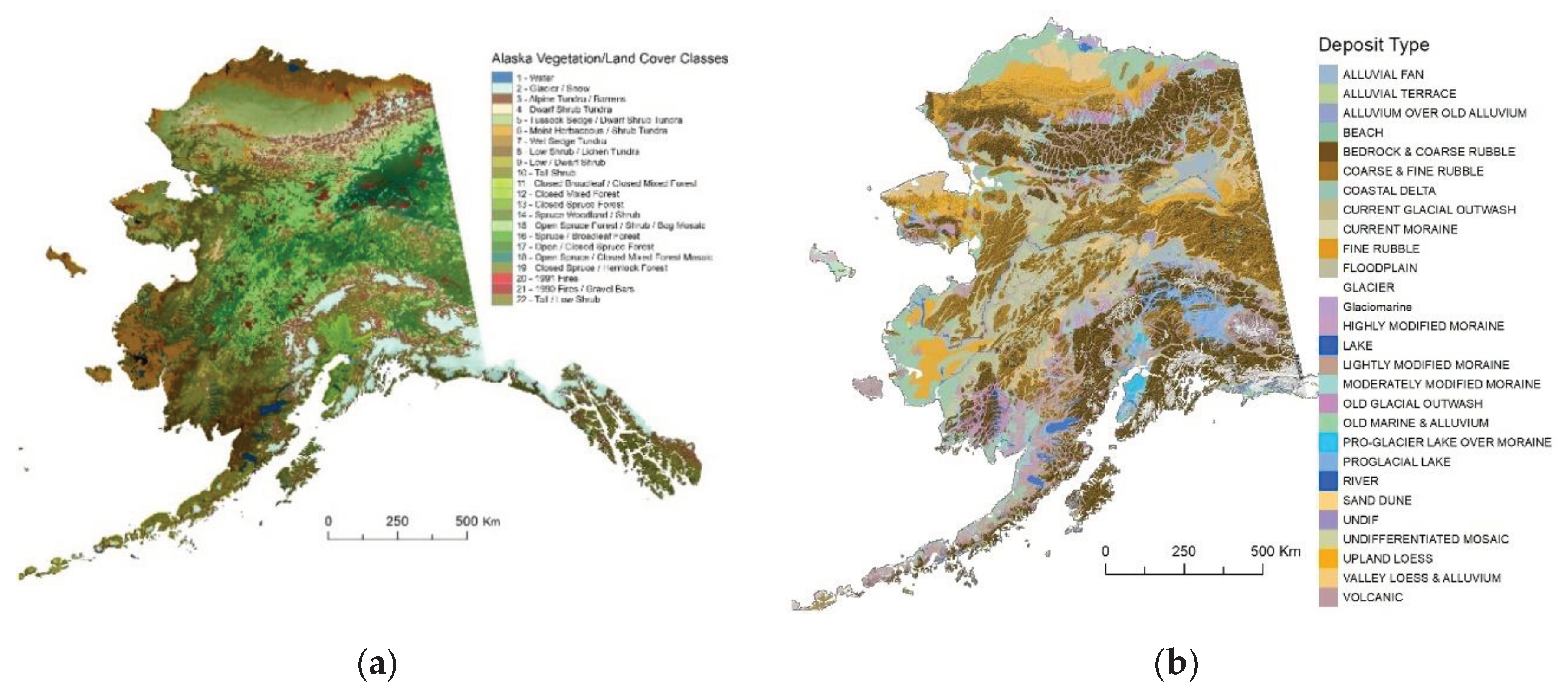
Figure 6.
Excess ice volume in top 5 m (a) based on surficial geology relationships [36]. Depth to bedrock (b) [47] compiled by Reginald Muskett, GI, UAF.
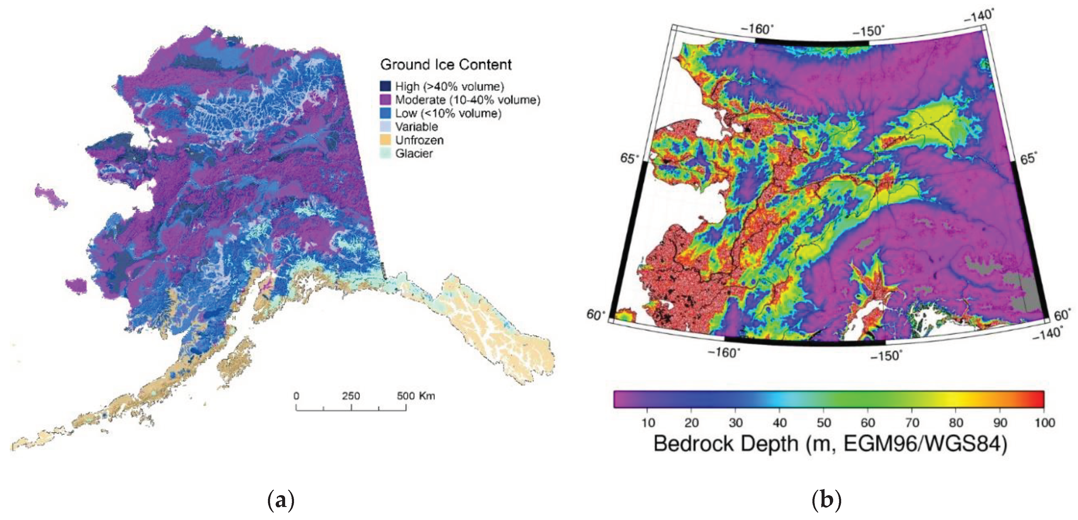
Figure 7.
(a) The general view of the landscape settings of the West Dock Oil Field specific site at Prudhoe Bay, north slope of Alaska, which is representing the Arctic Tundra Ecotype; (b) map of permafrost observing GTN-P site locations along the Alaskan Permafrost-Ecological Transect; (c) is an example of the GIPL2-MPI model calibration for the specific site West Dock, north slope of Alaska. (Photo: S. Marchenko).
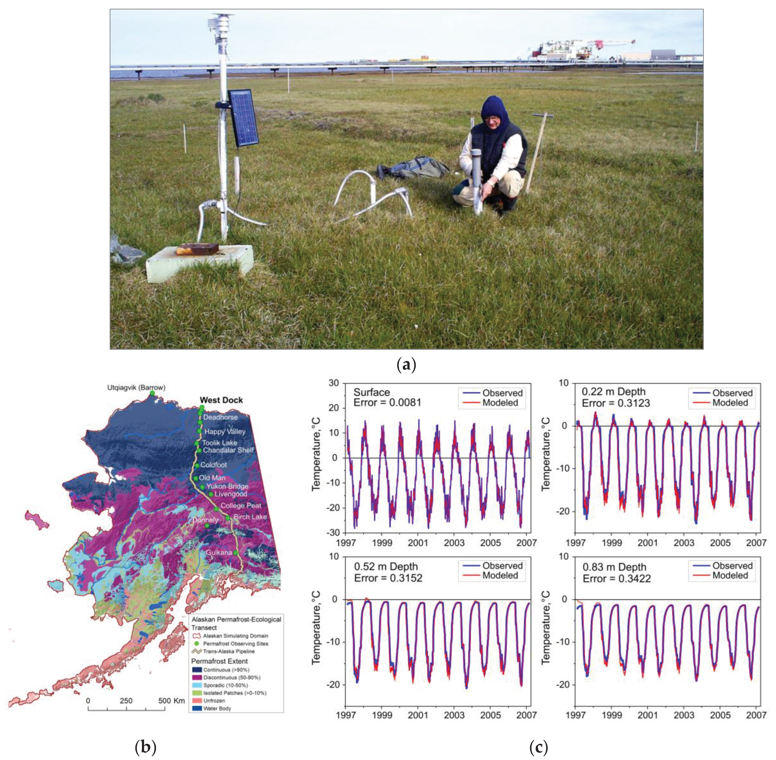
Figure 8.
(a) General view of the landscape settings and surface conditions of the Council Tundra (COT) permafrost observing site; (b) result of the GIPL2-MPI model calibration for the non-acidic Tundra ecotype at the Seward Peninsula, Alaska COT specific site. (Photo: S. Marchenko).
Figure 8.
(a) General view of the landscape settings and surface conditions of the Council Tundra (COT) permafrost observing site; (b) result of the GIPL2-MPI model calibration for the non-acidic Tundra ecotype at the Seward Peninsula, Alaska COT specific site. (Photo: S. Marchenko).
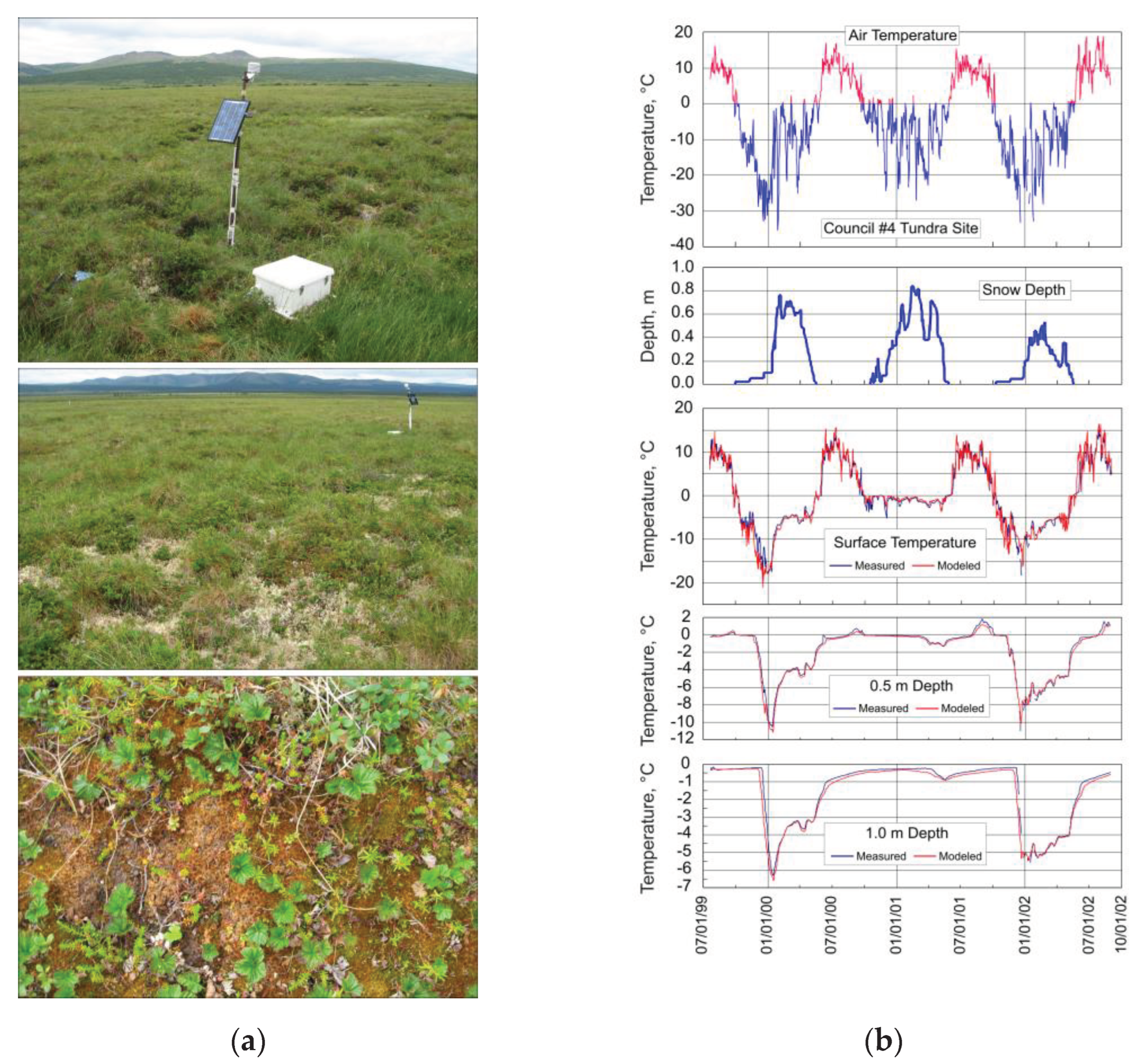
Figure 9.
(a) Landscape settings of the shrubland ecotype, interior Alaska; (b) result of the GIPL2-MPI model calibration for the specific site Council Shrubland (COS) within the shrubland ecotype at the Seward Peninsula, Alaska. (Photo: S. Marchenko).
Figure 9.
(a) Landscape settings of the shrubland ecotype, interior Alaska; (b) result of the GIPL2-MPI model calibration for the specific site Council Shrubland (COS) within the shrubland ecotype at the Seward Peninsula, Alaska. (Photo: S. Marchenko).
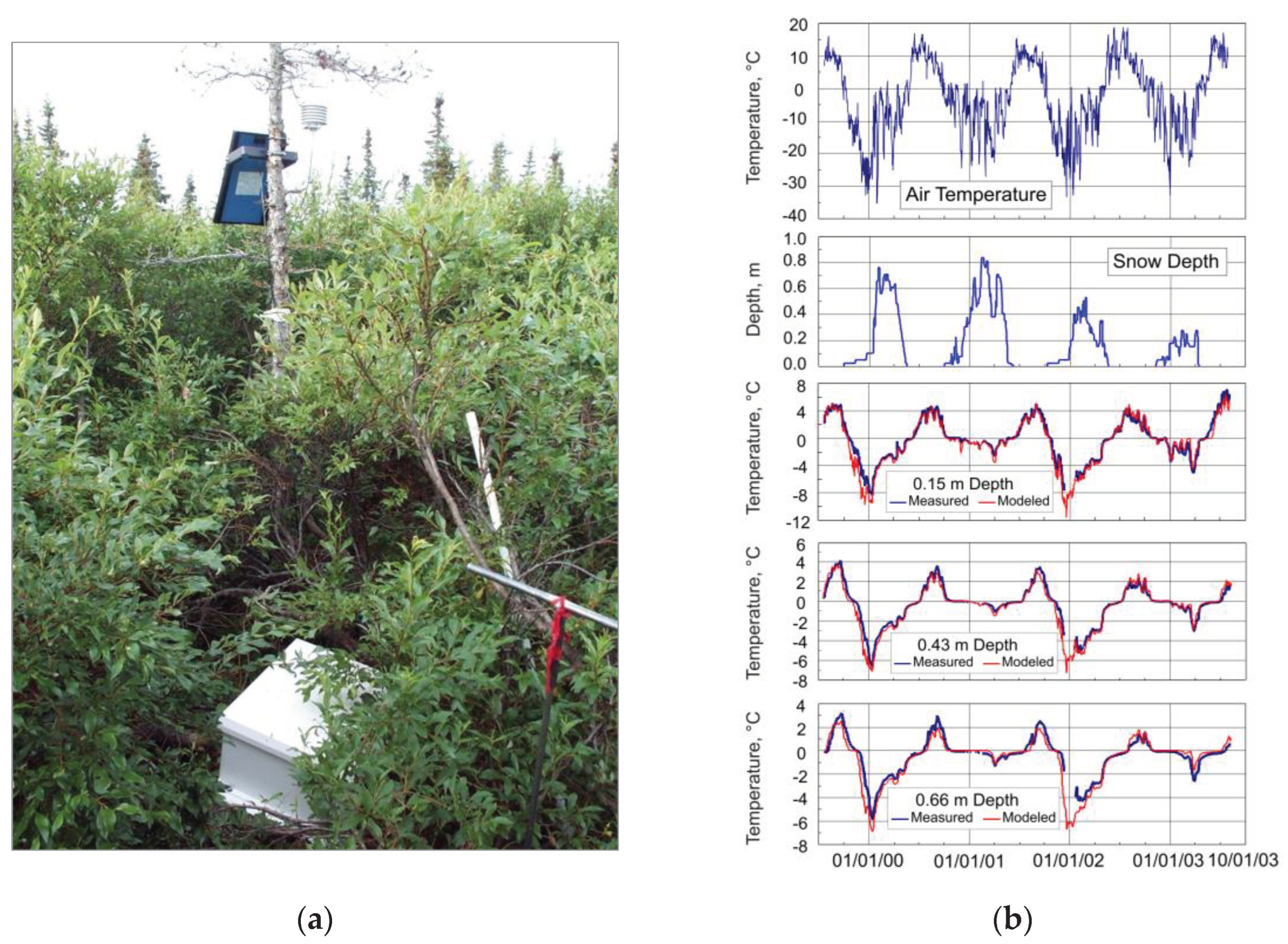
Figure 10.
(a) General view of the landscape settings and (b) surface conditions of the Washington Creak (WC1) Black Spruce permafrost observing site; (c) result of the GIPL2-MPI model calibration for the black spruce ecotype, interior Alaska, Fairbanks vicinity. (Photo: S. Marchenko).
Figure 10.
(a) General view of the landscape settings and (b) surface conditions of the Washington Creak (WC1) Black Spruce permafrost observing site; (c) result of the GIPL2-MPI model calibration for the black spruce ecotype, interior Alaska, Fairbanks vicinity. (Photo: S. Marchenko).
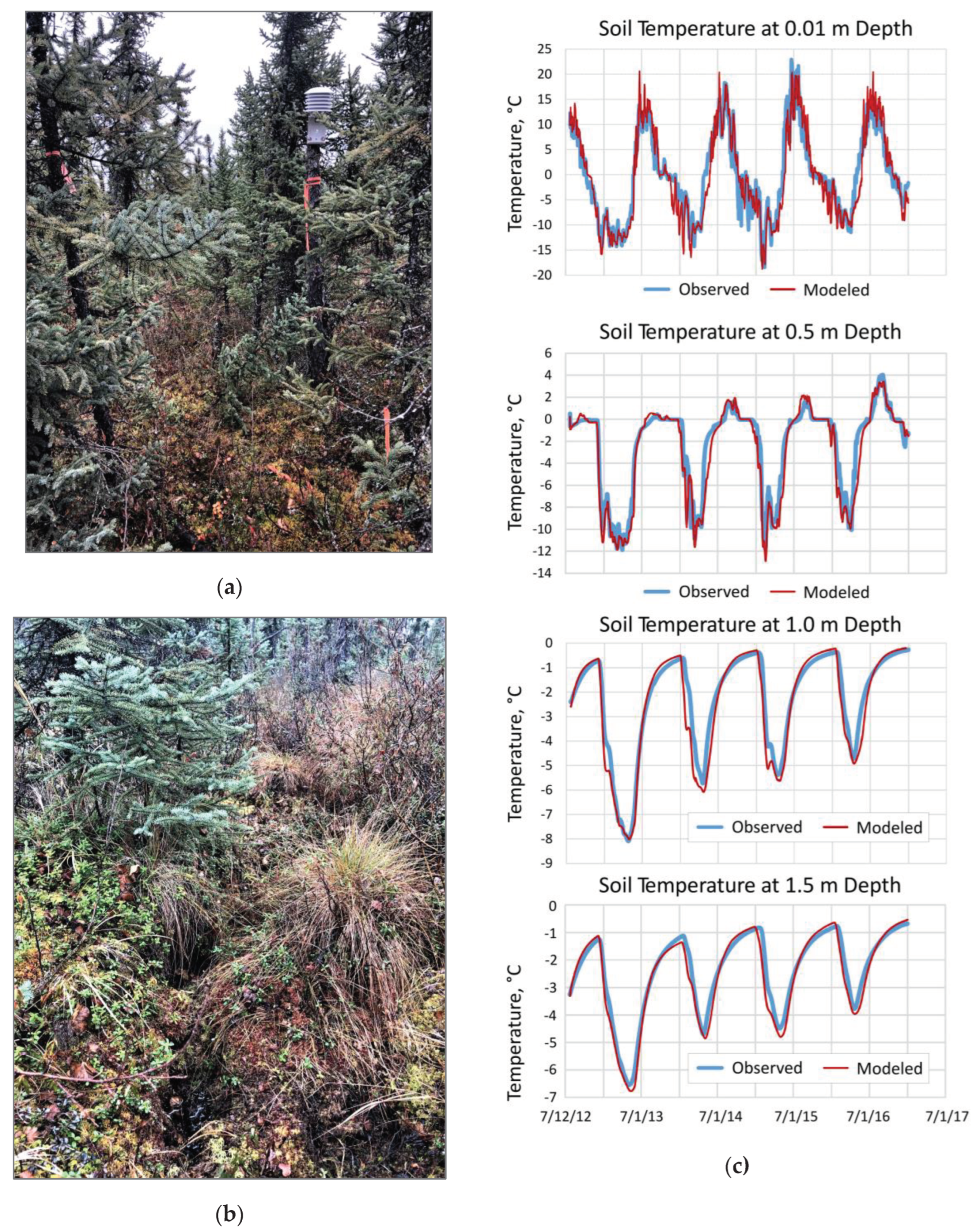
Figure 11.
Comparison of the average modeled and observed (a) MAGT and (b) ALT at the permafrost observing sites across Alaska (Figure 7b).
Figure 11.
Comparison of the average modeled and observed (a) MAGT and (b) ALT at the permafrost observing sites across Alaska (Figure 7b).
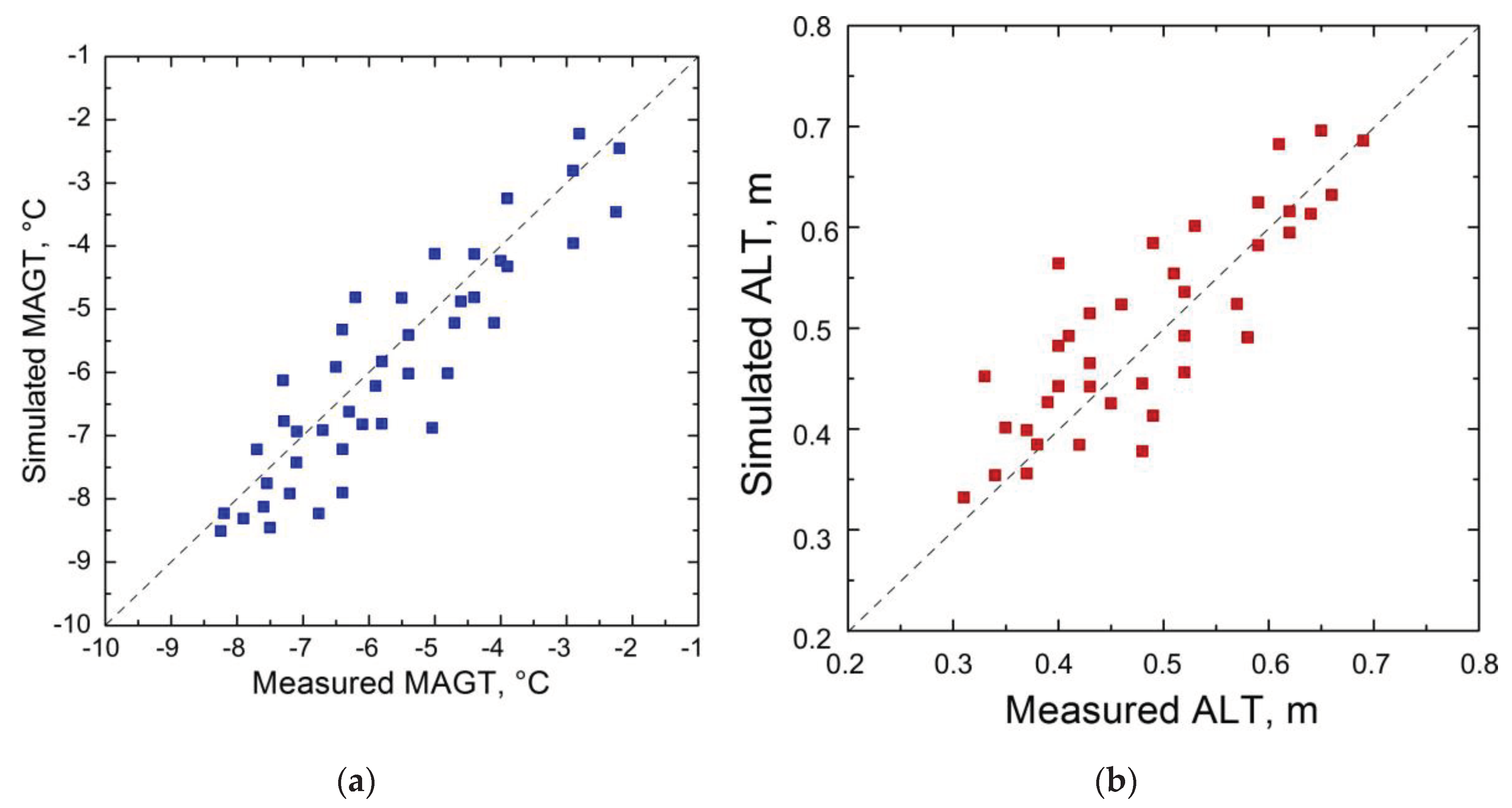
Figure 12.
(a) The general view of Smith Lake observing site (SL2), which represents black spruce ecotype, interior Alaska; (b) the sensitivity of the GIPL2_MPI modeled MAGT at 1 m depth averaged for 2000-2018 and averaged ALT for the same period on changes in the volumetric water content (VWC) and thermal conductivity for (c) thawed and (d) frozen soil layer of 0.25-1.0 m depth for the SL2 site.
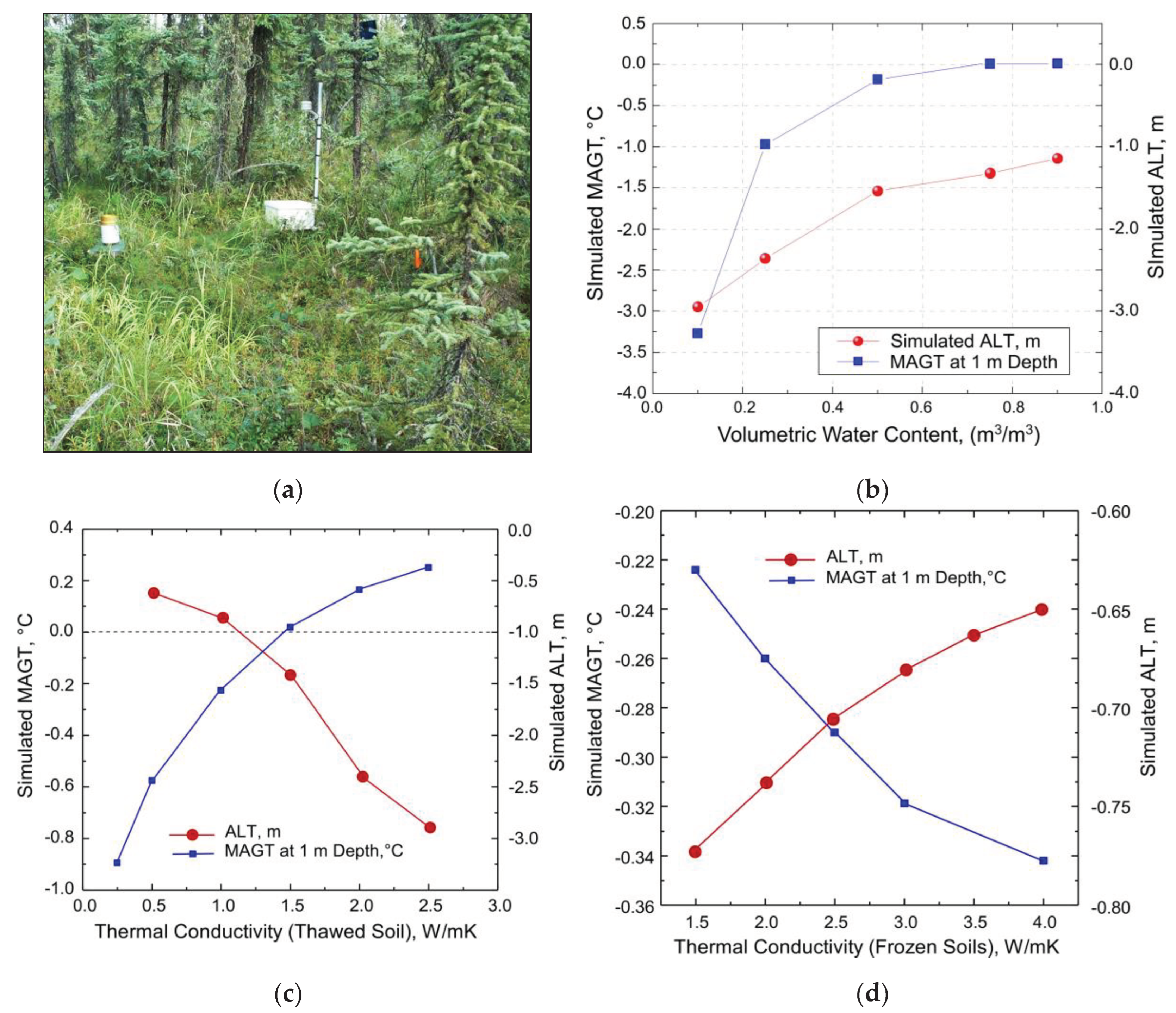
Figure 13.
Simulated site-specific MAGT dynamics at 2 m depth, according to the Five-Model Average climate forcing for the (a) RCP-4.5 and (b) RCP-8.5 scenarios.
Figure 13.
Simulated site-specific MAGT dynamics at 2 m depth, according to the Five-Model Average climate forcing for the (a) RCP-4.5 and (b) RCP-8.5 scenarios.
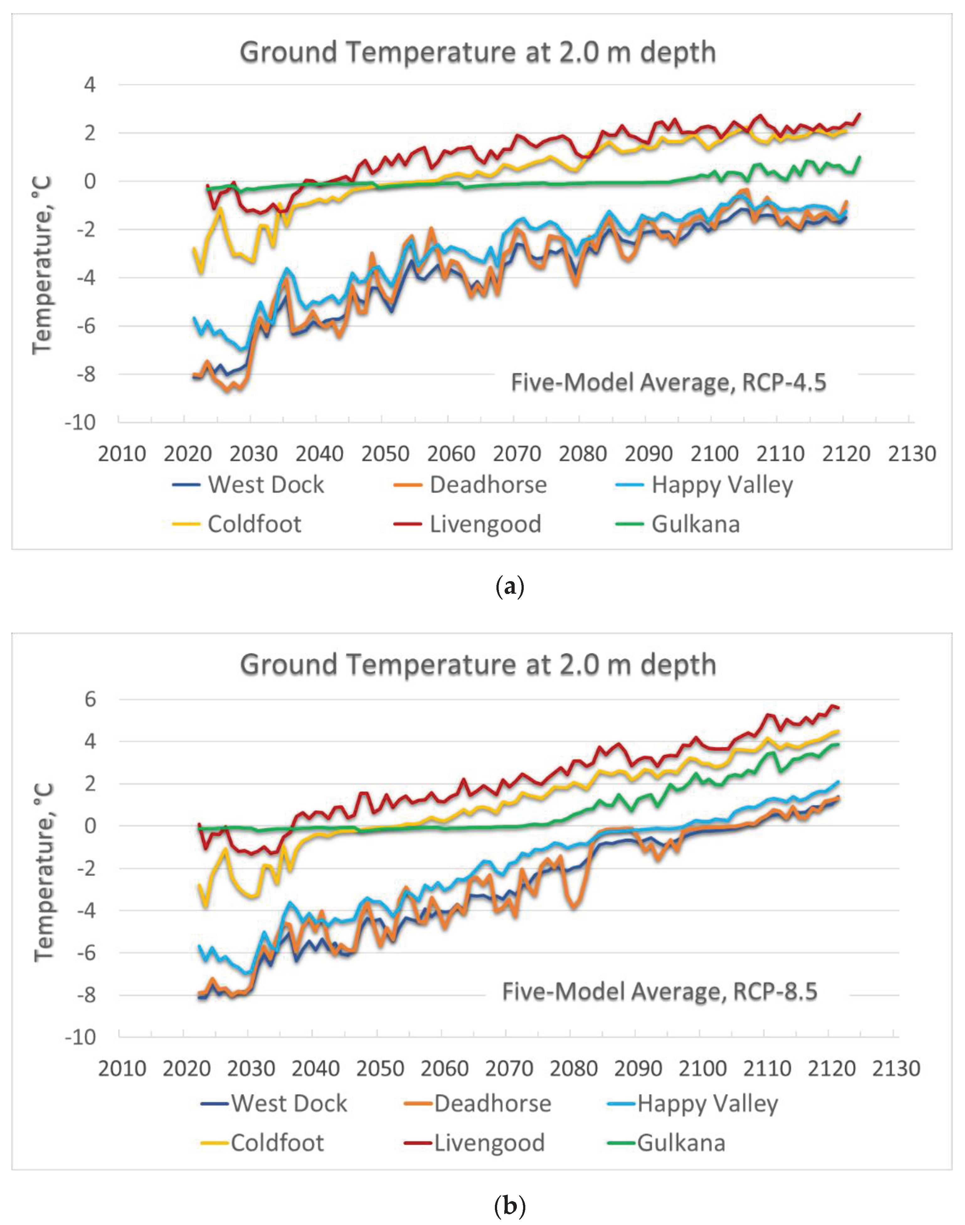
Table 2.
The reconstructed ground thermal properties for various soil types and major ecosystem classes across Alaska.
Table 2.
The reconstructed ground thermal properties for various soil types and major ecosystem classes across Alaska.
| Heat Capacity | Thermal Conductivity | |||||
| VWC*, | Thawed, | Frozen, | Thawed, | Frozen, | Depth, m | Layer matter (description) |
| m3 m-3 | J m-3 K-1 | J m-3 K-1 | W m-1 K-1 | W m-1 K-1 | ||
| Sub-polar or polar grassland-lichen-moss | ||||||
| 0.694 | 1.72d6 | 1.21d6 | 0.242 | 0.895 | 0.0-0.12 | moss |
| 0.696 | 1.93d6 | 1.51d6 | 0.452 | 1.032 | 0.12-0.22 | peat 1 (shallow organic, fibrous) |
| 0.583 | 2.02d6 | 1.65d6 | 0.524 | 1.056 | 0.22-0.68 | peat 2 (deep organic, amorphous) |
| 0.456 | 2.54d6 | 1.72d6 | 1.023 | 1.516 | 0.68-5.6 | mineral 1, silt |
| 0.442 | 2.93d6 | 2.23d6 | 1.216 | 1.645 | 5.6-8.8 | mineral 2, silty loam |
| 0.426 | 3.43d6 | 2.83d6 | 1.424 | 1.849 | 8.8-48.5 | mix of silt, gravel, sand, debris |
| 0.384 | 3.63d6 | 3.12d6 | 1.832 | 2.214 | 48.5-58.0 | gravel, coarse sand, debris |
| 0.071 | 3.85d6 | 3.46d6 | 2.502 | 2.589 | 58.0-100.0 | Bedrock |
| Bare mineral soil | ||||||
| 0.482 | 2.51d6 | 1.71d6 | 1.234 | 2.123 | 0.0-3.2 | mineral 1, silt |
| 0.356 | 1.83d6 | 1.63d6 | 2.134 | 2.821 | 3.2-18.5 | mineral 2, silt |
| 0.082 | 1.92d6 | 1.66d6 | 2.232 | 2.865 | 18.5-100.0 | Bedrock |
| Deciduous forest | ||||||
| 0.384 | 1.8d6 | 1.6d6 | 0.121 | 0.123 | 0.0-0.09 | Litter |
| 0.484 | 1.8d6 | 1.6d6 | 0.152 | 0.286 | 0.09-0.16 | peat 1 (shallow organic, fibrous) |
| 0.532 | 1.9d6 | 1.7d6 | 0.265 | 0.384 | 0.16-0.21 | peat 2 (deep organic, amorphous) |
| 0.416 | 2.2d6 | 2.1d6 | 1.101 | 1.542 | 0.21-0.6 | mineral 1, silt |
| 0.405 | 2.5d6 | 1.8d6 | 1.213 | 1.854 | 0.6-3.1 | mineral 2, silty loam |
| 0.341 | 1.8d6 | 1.6d6 | 2.215 | 2.865 | 3.1-63.5 | mix of silt, gravel, sand, debris |
| 0.076 | 1.8d6 | 1.6d6 | 2.321 | 2.845 | 63.5-100.0 | Bedrock |
| Mixed Forest | ||||||
| 0.384 | 1.8d6 | 1.6d6 | 0.094 | 0.134 | 0.0-0.03 | Litter, moss |
| 0.556 | 1.8d6 | 1.6d6 | 0.134 | 0.254 | 0.03-0.11 | peat 1 (shallow organic, fibrous) |
| 0.587 | 1.9d6 | 1.7d6 | 0.225 | 0.365 | 0.11-0.27 | peat 2 (deep organic, amorphous) |
| 0.412 | 2.2d6 | 2.1d6 | 1.132 | 1.543 | 0.27-0.97 | mineral 1, silt |
| 0.375 | 2.5d6 | 1.8d6 | 1.143 | 1.842 | 0.97-42.2 | mineral 2, silt loam |
| 0.313 | 1.8d6 | 1.6d6 | 2.245 | 2.843 | 42.2-52.5 | mix of silt, gravel, sand, debris |
| 0.067 | 1.8d6 | 1.6d6 | 2.236 | 2.837 | 52.5-100.0 | Bedrock |
| Herb Fen | ||||||
| 0.354 | 2.8d6 | 2.1d6 | 0.324 | 0.425 | 0.0-0.03 | Grass |
| 0.562 | 2.3d6 | 1.9d6 | 0.445 | 0.684 | 0.45-0.95 | peat 1 (shallow organic, fibrous) |
| 0.762 | 2.9d6 | 1.9d6 | 0.523 | 1.124 | 0.95-2.65 | peat 2 (deep organic, amorphous) |
| 0.478 | 2.2d6 | 1.8d6 | 1.234 | 2.031 | 2.65-3.2 | mineral 1, silt |
| 0.453 | 2.2d6 | 1.8d6 | 1.243 | 1.925 | 3.2-45.0 | mineral 2, silty loam |
| 0.332 | 1.8d6 | 1.6d6 | 2.213 | 2.845 | 45.0-59.5 | mix of silt, gravel, sand, debris |
| 0.062 | 1.8d6 | 1.6d6 | 2.234 | 2.856 | 59.5-100.0 | Bedrock |
| Shrub | ||||||
| 0.284 | 1.8d6 | 1.6d6 | 0.124 | 0.224 | 0.0-0.05 | Grass |
| 0.593 | 2.5d6 | 1.9d6 | 0.321 | 0.663 | 0.05-0.15 | peat 1 (shallow organic, fibrous) |
| 0.562 | 1.9d6 | 1.7d6 | 0.534 | 1.012 | 0.15-0.27 | peat 2 (deep organic, amorphous) |
| 0.456 | 2.2d6 | 2.1d6 | 1.032 | 2.132 | 0.15-0.65 | mineral 1, silt |
| 0.384 | 2.2d6 | 1.8d6 | 1.043 | 1.945 | 0.65-48.6 | mineral 2, silt loam |
| 0.273 | 1.8d6 | 1.6d6 | 2.232 | 2.845 | 48.6-67.2 | mix of silt, gravel, sand, debris |
| 0.079 | 1.8d7 | 1.6d7 | 2.243 | 2.854 | 67.2-100.0 | Bedrock |
| Sphagnum Bog | ||||||
| 0.345 | 2.4d6 | 1.9d6 | 0.245 | 0.384 | 0-0.02 | Lichen |
| 0.512 | 2.5d6 | 1.9d6 | 0.446 | 0.782 | 0.02-0.12 | Moss |
| 0.624 | 2.45d6 | 1.85d6 | 0.412 | 0.865 | 0.12-0.55 | peat 1 (shallow organic, fibrous) |
| 0.742 | 2.9d6 | 1.9d6 | 0.523 | 1.132 | 0.55-1.1 | peat 2 (deep organic, amorphous) |
| 0.425 | 2.2d6 | 1.8d6 | 1.254 | 2.032 | 1.1-2.65 | mineral 1, silt |
| 0.407 | 2.2d6 | 1.8d6 | 1.234 | 1.954 | 2.65-48.2 | mineral 2, silt loam |
| 0.285 | 1.8d6 | 1.6d6 | 2.254 | 2.846 | 48.2-55.5 | mix of silt, gravel, sand, debris |
| 0.072 | 1.8d7 | 1.6d7 | 2.243 | 2.854 | 55.5-100.0 | Bedrock |
| Tussock Tundra | ||||||
| 0.386 | 1.8d6 | 1.6d6 | 0.224 | 0.384 | 0.0-0.03 | Grass, moss |
| 0.545 | 2.5d6 | 1.9d6 | 0.344 | 0.564 | 0.03-0.32 | peat 1 (shallow organic, fibrous) |
| 0.632 | 1.9d6 | 1.7d6 | 0.456 | 0.954 | 0.32-0.52 | peat 2 (deep organic, amorphous) |
| 0.554 | 2.2d6 | 2.1d6 | 0.932 | 2.132 | 0.52-0.68 | peat 3 (deep organic, amorphous) |
| 0.462 | 2.2d6 | 1.8d6 | 1.045 | 2.156 | 0.62-3.55 | mineral 1, silt |
| 0.354 | 1.8d6 | 1.6d6 | 2.234 | 2.658 | 3.55-65.5 | mineral 2, silt loam |
| 0.093 | 1.8d7 | 1.6d7 | 2.654 | 2.865 | 65.5-100.0 | Bedrock |
| White Spruce | ||||||
| 0.545 | 1.8d6 | 1.6d6 | 0.084 | 0.134 | 0.0-0.06 | Moss |
| 0.586 | 1.9d6 | 1.7d6 | 0.125 | 0.226 | 0.06-0.12 | peat 1 (shallow organic, fibrous) |
| 0.565 | 1.9d6 | 1.7d6 | 0.267 | 0.456 | 0.12-0.3 | peat 2 (deep organic, amorphous) |
| 0.447 | 2.2d6 | 2.1d6 | 1.268 | 1.547 | 0.3-0.85 | mineral 1, silt |
| 0.448 | 2.5d6 | 1.8d6 | 1.278 | 1.952 | 0.85-25.5 | mineral 2, silt loam |
| 0.234 | 1.8d6 | 1.6d6 | 2.245 | 2.687 | 25.5-55.6 | mix of silt, gravel, sand, debris |
| 0.081 | 1.8d7 | 1.6d7 | 2.654 | 2.875 | 55.6-100.0 | Bedrock |
| Willow | ||||||
| 0.336 | 1.8d6 | 1.6d6 | 0.146 | 0.287 | 0.0-0.05 | Grass |
| 0.524 | 1.8d6 | 1.6d6 | 0.245 | 0.489 | 0.05-0.22 | peat 1 (shallow organic, fibrous) |
| 0.656 | 1.9d6 | 1.7d6 | 0.368 | 0.765 | 0.22-0.35 | peat 2 (deep organic, amorphous) |
| 0.528 | 2.2d6 | 2.1d6 | 1.157 | 2.213 | 0.35-1.3 | mineral 1, silt |
| 0.512 | 2.5d6 | 1.8d6 | 1.065 | 1.965 | 1.3-3.5 | mineral 2, silt loam |
| 0.285 | 1.8d6 | 1.6d6 | 2.234 | 2.845 | 3.5-54.5 | mix of silt, gravel, sand, debris |
| 0.074 | 1.8d7 | 1.6d7 | 2.543 | 2.985 | 54.5-100.0 | Bedrock |
*VWC – volumetric water content;.
Disclaimer/Publisher’s Note: The statements, opinions and data contained in all publications are solely those of the individual author(s) and contributor(s) and not of MDPI and/or the editor(s). MDPI and/or the editor(s) disclaim responsibility for any injury to people or property resulting from any ideas, methods, instructions or products referred to in the content. |
© 2024 by the authors. Licensee MDPI, Basel, Switzerland. This article is an open access article distributed under the terms and conditions of the Creative Commons Attribution (CC BY) license (http://creativecommons.org/licenses/by/4.0/).
Copyright: This open access article is published under a Creative Commons CC BY 4.0 license, which permit the free download, distribution, and reuse, provided that the author and preprint are cited in any reuse.


