Submitted:
08 March 2024
Posted:
15 March 2024
Read the latest preprint version here
Abstract
This study presents an extensive collection of data on the aerodynamic behavior at a low Reynolds number and geometric coefficients for 2900 airfoils, obtained through the class shape transformation (CST) method. By employing a verified OpenFOAM-based CFD simulation framework, lift and drag coefficients were determined at a Reynolds number of 10^5. Considering the limited availability of data on low Reynolds number airfoils, this dataset is invaluable for a wide range of applications, including unmanned aerial vehicles (UAVs) and wind turbines. Additionally, the study offers a method for automating CFD simulations that could be applied to analyze higher Reynolds numbers. The breadth of this dataset also supports the enhancement and creation of machine learning (ML) models, further advancing research into the aerodynamics of airfoils and lifting surfaces.
Keywords:
airfoil
; computational fluid dynamics (CFD)
; OpenFOAM
; class shape transformation (CST)
; dataset
; aerodynamic coefficients
; geometric coefficients
; aerodynamics
1. Introduction and Background
Airfoils designed for low Reynolds numbers play crucial roles in various applications, including Mini Unmanned Aerial Vehicles (UAVs), which are instrumental in executing high-definition remote sensing, infrastructure surveillance, 3D mapping, and photogrammetry tasks [1,2,3]. Additionally, they are vital for Small-Scale Wind Turbines (SSWTs), contributing to the reduction of electrical grid demands and greenhouse gas emissions [4]. To maximize the performance of these technologies, the airfoils must be specifically designed to meet their unique requirements. Techniques for optimizing airfoil design frequently include the use of genetic algorithms, surrogate-based modeling, and artificial neural networks [5,6].
This study enhances the development of machine/deep learning approaches for airfoil optimization by generating a dataset with lift, drag, and parameterization coefficients for 2900 airfoils at a Reynolds number of . The lift and drag coefficients were generated using the CFD approach implemented in OpenFOAM [7]. The Class Shape Transformation (CST) method [8] was employed to describe the curve of each airfoil. Additionally, the CST method was applied to augment the point count in each airfoil’s ’.dat’ file, improving the accuracy of the mesh. The dataset also incorporates these refined coordinates from every ‘.dat’ file.
2. Methodology
2.1. Airfoil Profile
The initial airfoil ’.dat’ files were obtained from the UIUC Airfoil database [9] and the AirfoilTools [10] online databases. The ’.dat’ files thus obtained were of varying number of points, and hence, this was a major consideration during the automation of the Class Shape Transformation (CST) process. Only Selig format ’.dat’ files were used during the entirety of the study. Selig format ’.dat’ files are a common way of representing airfoil geometries in aerodynamics and aerospace engineering. Each line in a Selig format ’.dat’ file represents a coordinate pair (x, y) of a point on the airfoil surface. The first point is typically located at the leading edge of the airfoil (0,0), and subsequent points follow in sequence towards the trailing edge along the x-axis.
2.2. Class Shape Transformation (CST) Parametrization Technique
The Class Shape Transformation (CST) parametrization technique was developed by Brenda Kulfan [8], an aerodynamic engineer at Boeing, in 2008. It incorporates a geometric class/shape function transformation technique.
2.2.1. Fundamental Approach
The general form of the mathematical expression that represents a typical airfoil geometry is:
where , and . The term corresponds to the round nose of the airfoil. Similarly, the term corresponds to the sharp trailing edge of the airfoil. The term controls the thickness of the trailing edge, and the summation term is a general function that describes the shape of the airfoil between the round nose and the sharp trailing edge.
2.2.2. CST Parameters
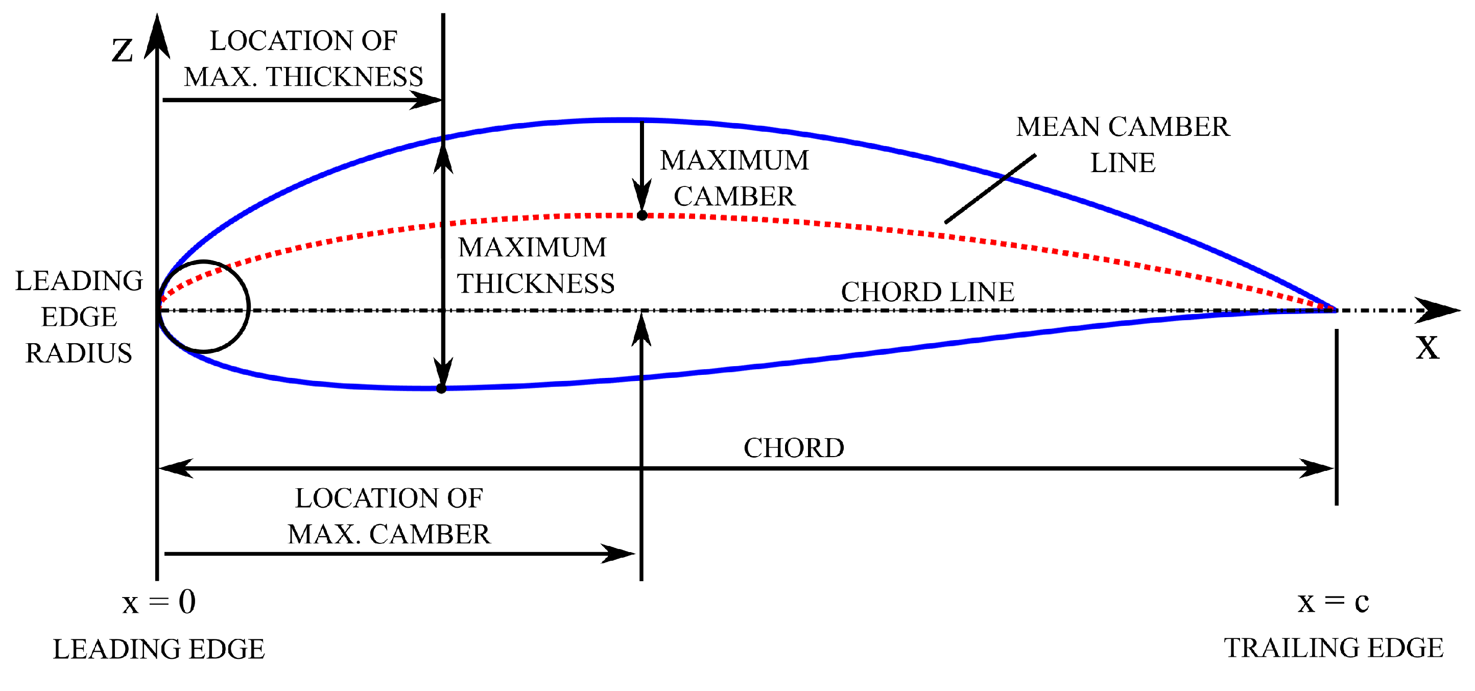
The CST parameters are given as follows (Adapted from [11]),
Figure 1.
CST Parameters
2.2.3. Airfoil Shape & Class Function
The shape function is given by the relation,
The term defines the class function given by,
Generally, for a round-nose airfoil, the values of N1 and N2 are 0.5 and 1, respectively. The class function is used to define general classes of geometries, whereas the shape function is used to define specific shapes within a class of geometries. Defining an airfoil shape function and specifying its geometry class is equivalent to defining the actual airfoil coordinates, which can then be obtained from the combination of the shape and class functions from the relation,
The airfoil is then defined using the Bernstein polynomials, which are defined for the order n as follows,
The binomial coefficients are defined as,
The first term of the polynomial defines the leading-edge radius, and the last term is the boat-tail angle. The other terms in between are the "shaping terms". In our case, we take a Bernstein polynomial of the eighth order, and hence, eight weighted coefficients are obtained at the end of the CST process. The upper surface of the airfoil is defined by the equations,
The lower surface of the airfoil is defined by the equations,
where,
The drag predictions and pressure distribution for a Bernstein’s polynomial of the 8th order agree exactly with experimental data, and hence, a Bernstein polynomial of the 8th order was chosen.
2.2.4. Notable Observations
During the airfoil parameterization process, some significant observations were made that are worth mentioning. There was a significant increase in the error percentage of the airfoil generated using the CST method when a y-offset existed in the leading edge point from (0,0). This produced a significant change in the curvature of the airfoil, which the ’blockMesh’ utility would not be able to capture. There was also a considerable number of airfoils with trailing edges not at (1,0). This poses a considerable challenge to meshing since one of the requirements for meshing was a trailing edge at (1,0). Such airfoils were removed from the initial airfoils database. There is a minimal margin of error between the original and the obtained airfoils. This framework was implemented in MATLAB®.
2.2.5. Shape Generation
Below are some plots of various airfoil sections generated using the CST framework.
Figure 2.
Plots of CST of Varied Airfoil Sections

2.3. Geometry
The length of the airfoil generated by the CST framework was standardized to be 1m. Increasing the number of points on the ".dat" file would invariably increase the accuracy of the simulations as they better represent the shape of the airfoil. The CST code provides the ".dat" file with the required number of equally distributed coordinates. Simulations were carried out for airfoils with 100, 300, 600, and 2000 points. It was found that beyond 600 points, the number of coordinates no longer influenced the simulation results. Subsequently, 600-point ".dat" files were standardized for future simulations. The computational domain featured a C-type topology with an average far-field separation of 11 chord lengths. The curved surface, along with the top and bottom surfaces, were given the flow inlet boundary condition, while the right-side wall was given the outlet condition.
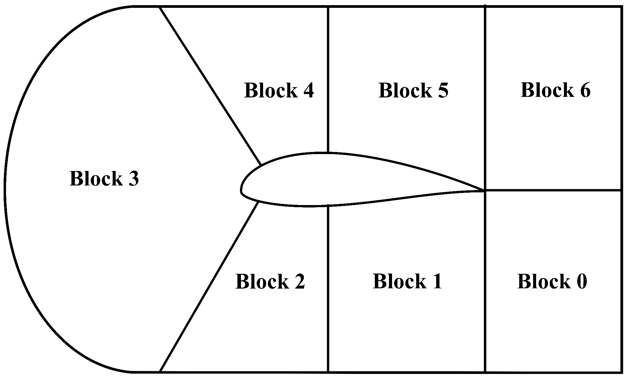
The domain consists of 7 blocks, with the blocks numbered 0, 1, and 2 being mirror images of the domains 6, 5, and 4, respectively, across the airfoil chord line. All the airfoil coordinates were linked using the OpenFOAM ’polyLine’ segments. Since the ’polyline’ edges did not satisfactorily capture the curvature of the airfoil leading edge, a separate block was created (block 3) with the airfoil coordinates joined using the OpenFOAM ’Spline’ curve segments.
Figure 3.
Computational Domain
2.4. Mesh
The OpenFOAM ’blockMesh’ mesh generation utility was used in this paper. Firstly, a mesh independence study was carried out to determine the influence of the number and size of mesh cells on the simulation result. Generally, the greater the number of cells, the higher both the simulation accuracy and computational time and resources. This grid independence study is performed by comparing the lift coefficient of the symmetric NACA 0018 airfoil at 4°AoA.
Figure 4 revealed that a grid consisting of 198,000 cells would be sufficient to establish a grid-independent solution. These 198,000 structured hexahedral cells were divided into a far-field and a more refined Near-field region. Multi-grading techniques were also used to control the expansion ratios of the cells within the blocks and to make the boundary layer region close to the airfoil wall especially refined. The aspect ratio of the cells close to the airfoil was controlled so that they were well within the acceptable limits as high-aspect ratio cells, especially in the flow-sensitive regions, sometimes affect the legitimacy of the results.
2.5. Solver and Turbulence Model
The simulations were run using the steady-state Reynolds-Averaged Navier-Stokes (RANS) OpenFOAM ’simpleFOAM’ solver along with the viscous Spalart-Allmaras turbulence model. The simpleFOAM solver is a pressure-based solver (for low-speed incompressible flows) that incorporates the SIMPLE (Semi-Implicit Method for Pressure-Linked Equations) algorithm. This solver is generally preferred to other pressure-based OpenFOAM solvers (such as PisoFoam or PimpleFoam) for largely incompressible and turbulent flows around airfoils.
The Spalart-Allmaras model is a single-equation turbulence model, solving for the modified turbulent kinematic viscosity, is widely used in various aerospace applications, and is designed for low-velocity wall-bounding flows with boundary layers subject to adverse pressure gradients like in airfoils. It is commonly used for low-Reynolds number flows and is more straightforward to implement, unlike other turbulence models such as the k- or the k- models, which require the turbulent length scale to be calculated. The Spalart-Allmaras transport equation, solving for the turbulent kinematic viscosity, , is given below:
The turbulent viscosity, can be determined through:
Subsequently, the viscous damping function, is given by:
X represents the ratio of the turbulent kinematic viscosity to the kinematic viscosity:
The empirical constants for the Spalart-Allmaras model are given by: , , , , , , , , , .
The kinematic viscosity () for the domain is assumed to be . For the Spalart-Allmaras model, the turbulent viscosity () is initialized to be equal to the kinematic viscosity in the internal field of the domain while the turbulent kinematic viscosity () is initialized to be equal to (X = 4).
2.6. Automation
Automating the process of generating the dataset was a critical part of the study. This was accomplished using a multifaceted approach. The software (in order of usage) used during the automation process are given by Figure 6.
The CST framework was developed in MATLAB®. Python was used to automate the mesh generation. Bash scripts were used to automate the process of running the CFD simulations. Further, Python was used for the post-processing of the results. The final approach used is given by Figure 7.
2.6.1. Automation of CST Using MATLAB®
The process of generating the CST coefficients and the 600-point ’.dat’ files was automated using MATLAB®. Figure 8 outlines the step-by-step process of how this was achieved.
2.6.2. Mesh Generation
A standardized BlockMeshDict file was initially created to automate the airfoil meshing process. Subsequently, a Python script was developed to extract coordinates from an airfoil ’.dat’ file and systematically substitute them into their designated lines within the BlockMeshDict file. This facilitated the meshing of any 600-point Selig format ’.dat’ file.
2.7. Bash Scripting
Bash scripts played a crucial role in the study. They were used throughout multiple stages of the simulation, right from the case setup to the post-processing of the results obtained. They were also used extensively in the parallelization process of the CFD simulations and are used to control the multiple simulations running in parallel.
2.7.1. CFD Automation
It was determined from multiple simulations that 2000 iterations were sufficient to achieve a near-converged solution, with the final residuals for all the parameters (U, p, and the turbulence parameters) approximately being in the order of . Increasing the number of iterations further, which would substantially increase the computational time and resources, no longer influenced the parameters measured. Subsequently, for the simulation automation process, the number of iterations for each airfoil was capped at 2000.
2.7.2. Parallelization
The version of OpenFOAM used during the entirety of the study was OpenFOAM v2306. The simpleFOAM solver used for the simulations is primarily a CPU-based solver. The simulations were initially carried out on a laptop with a Ryzen 7 5800H CPU with 32 GB RAM. The aforementioned CPU has eight cores and 16 threads. A simulation run using a single core took roughly 20 minutes. By this accord, it would take roughly 42 days to run simulations of all the airfoils for a single AoA. Due to the sheer amount of time it would take to run simulations for a single AoA, it was then decided to parallelize the process of simulation.
After initially parallelizing the simulations on the aforementioned laptop, the cases were then initially copied to a supercomputer with an AMD Epyc 32-core CPU and 110 GB RAM. The database of airfoils was split into parts. One case from each of these subdatabases would then be run in parallel. In essence, at any given time, there would be multiple simulations running in parallel. The optimum number of simulations to be run in parallel was arrived at after trying out various cases and monitoring the supercomputer performance and the combined time of simulations (one AoA).
After several iterations to the parallelization setup, the final case was run on 4 Intel Xeon Platinum 8268 processors with a total of 96 cores and 1,536 GB RAM. The database was split into 96 parts, and the final simulation time for one AoA was found to be roughly 2 days.
2.7.3. Post-Processing
A Python script was developed to store the results of the simulation along with the AoA and the CST coefficients in a comma-separated values file (.csv). This was done to consolidate the data obtained and for the ease of future data analysis.
3. Data Description
The dataset is stored on a GitHub repository. The data structure of the repository is given by Figure 9.
The repository is primarily divided into 5 parts. These correspond to the raw and processed airfoil data, the CFD and CST subdirectories, and the final dataset. The CFD subdirectory contains the OpenFOAM case setup and its associated directories. Similarly, the CST subdirectory contains the CST framework. Further, separate directories have been created for the raw and processed airfoil databases. The format of the dataset is elucidated in Table 1. AoA refers to the angle of attack, the CST coefficients, and , are the lift and drag coefficients, respectively.
4. Data Validation
The lift and drag coefficients of select symmetric and cambered airfoils were validated by comparing the simulated results with experimental data from two references around the selected Reynolds number of 100,000. To conclusively demonstrate the accuracy of the results and the simulation, multiple types of airfoils were compared, though only a few relevant figures are presented for space constraints. NACA airfoils were validated using the NACA report [12] while other non-NACA were validated with data available from the literature book reference [13].
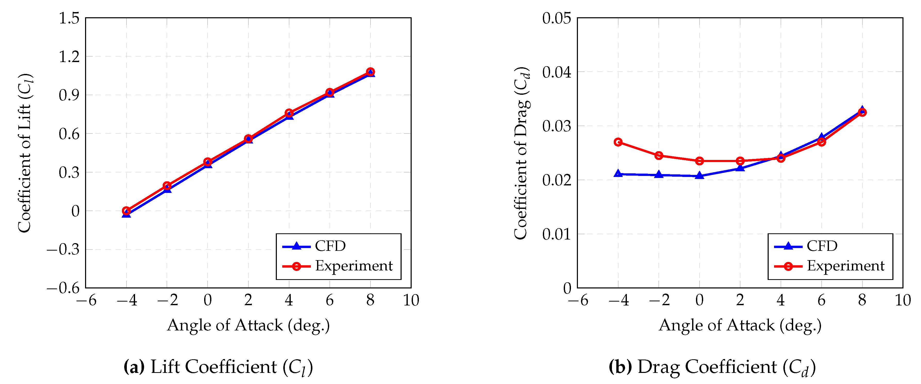
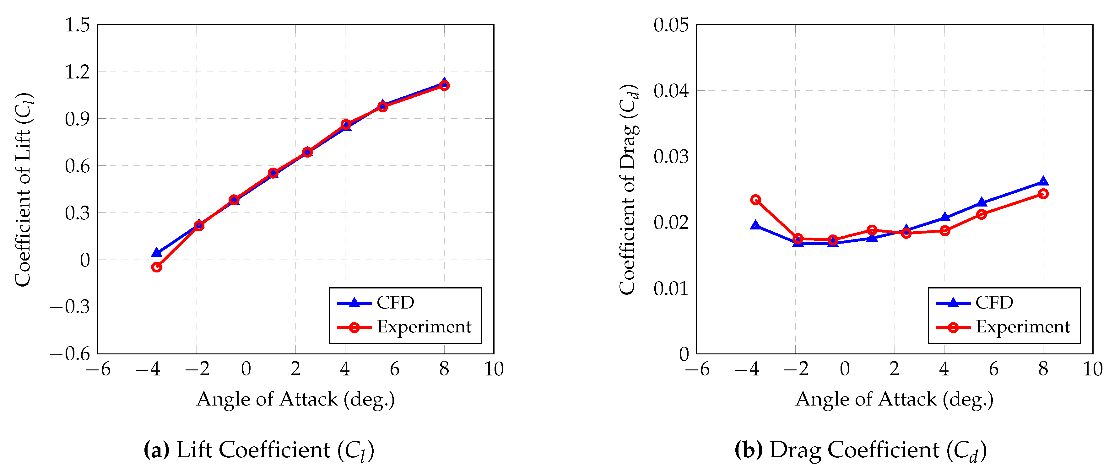
The numerically obtained and experimental lift and drag coefficients for one symmetric test airfoil, the NACA 0018 at a Reynolds number of 84,000, and one cambered airfoil, the NACA 2412 at a Reynolds number of 82,800 are illustrated in Figure 10 and Figure 11.
The OpenFOAM model predicts the values across the chosen AoA range, like the experimental results. The percentage errors for both the lift and drag coefficients lie within 5% for the symmetric NACA 0018, hence producing highly accurate results. For the cambered NACA 2412 airfoil, the lift coefficient predictions are within 5% of the experimental values too. However, the OpenFOAM simulations under-predict the drag coefficients for NACA 2412 by approximately 15% at some AoAs. Similar trends were observed while validating the other test airfoils, which showed accurate lift coefficients yet slightly under-predicted drag values. The aerodynamic coefficients of the NACA 4415 and NACA 6412 airfoils at Reynolds numbers of 82,500 and 83,000 respectively are illustrated below. While the values can be obtained within 5% margin of error, the discrepancy between the numerical and experimental values exceeds 10% at high and especially negative angles of attack.
Figure 12.
Aerodynamic characteristics of NACA 4415
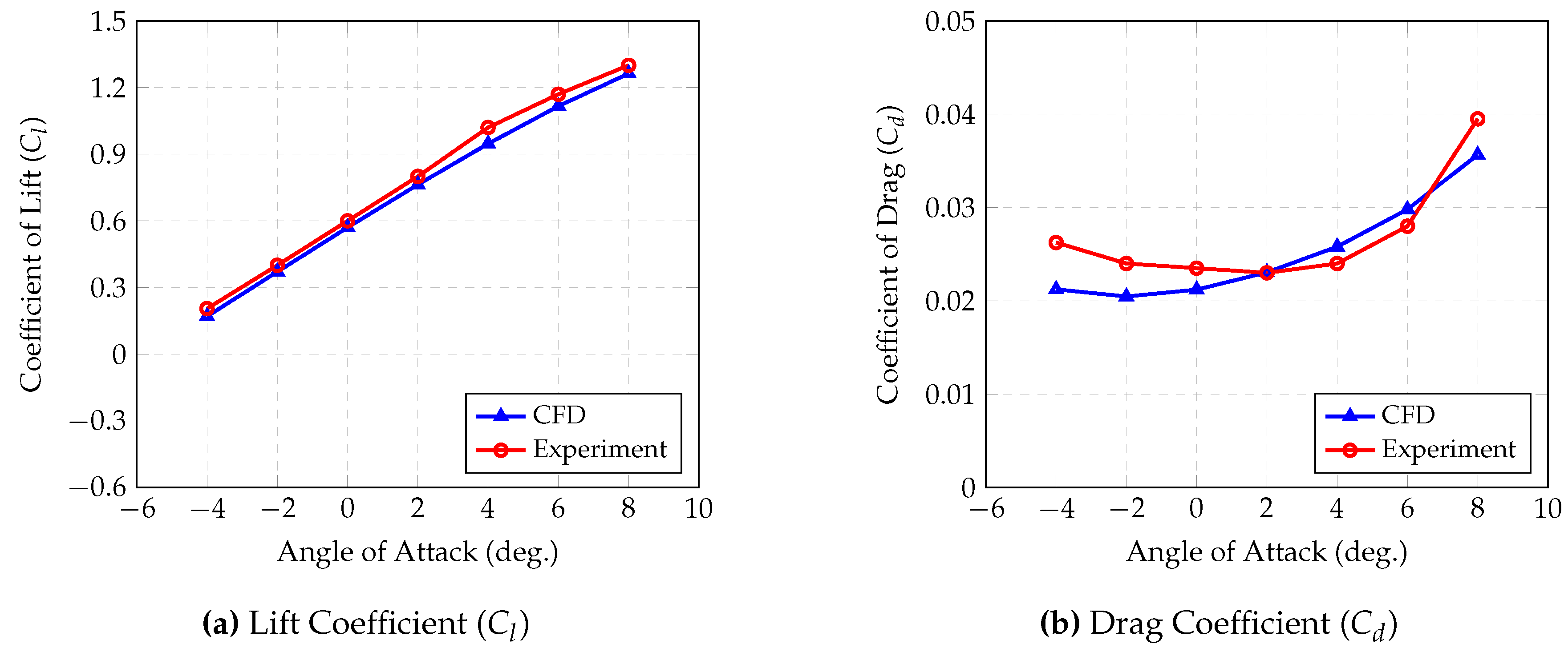
Figure 13.
Aerodynamic characteristics of NACA 6412
Validation was also carried out for non-NACA airfoils. The results obtained for the Selig/Donnovan SD8020 airfoil at a Reynolds number of 101,800 is shown below. Expected results were obtained; the error in the lift is less than 4% while the error in the drag coefficient remains less than 10% apart from at highly negative angles of attack.
Figure 14.
Aerodynamic characteristics of SD 8020
It is difficult to accurately predict the aerodynamic behavior, especially drag, in regions of highly separated flow or at high angles of attack using numerical methods [14]. Subsequently, the simulation values start to diverge from the literature values as the angle of attack approaches the extremities (detached flows) and is generally difficult to prevent unless unsteady RANS or Large Eddy Simulation (LES) simulation methods and extremely refined meshes are implemented [15]. The discrepancy between the numerical and experimental and results across AoA using the Spalart Allmaras model has been documented before by this study [16].
While the numerical OpenFOAM results sometimes under-predict the drag forces, the current lift and drag predictions within our required angles of attack (without dominant flow separation) are sufficient for our current study. Furthermore, the high accuracy obtained from the simulations across different references also validates the proof of concept of the automated simulations.
5. Conclusions
This paper introduces a dataset featuring airfoil aerodynamic coefficients and CST parameters of airfoils obtained from reputable online repositories (the UIUC Airfoil Database and AirfoilTools). Focused on low Reynolds numbers (100,000), it serves as a proof of concept of a robust and automated framework for CFD analyses. The release of both the CFD framework and dataset sets the stage for future research, including expansion to higher Reynolds numbers and the training of several AI models for low Reynolds number aerodynamic analyses. This dataset could serve as a valuable resource for researchers and engineers in various fields.
Author Contributions
Conceptualization, M.M.; Methodology, M.M., V.V., K.A., and D.M.; Validation, V.V.; Automation, K.A. and D.M.; Data Collection, K.A.; Writing – Original Draft Preparation, V.V., K.A. and D.M.; Writing – Review & Editing, V.V., K.A. and D.M.; Visualization, K.A. All authors have read and agreed to the published version of the manuscript.
Funding
This research received no external funding.
Institutional Review Board Statement
Not applicable.
Informed Consent Statement
Not applicable.
Data Availability Statement
The dataset, along with the framework used to generate the dataset, can be found on the GitHub repository (https://github.com/kanakaero/Dataset-of-Aerodynamic-and-Geometric-Coefficients-of-Airfoils.git).
Acknowledgments
We would like to acknowledge the support of the Computer Science Engineering Department at the Manipal Institute of Technology, MAHE, Manipal, Karnataka, India, for giving us access to their supercomputer, "MIT Cloud GPU". We would also like to acknowledge the National Supercomputing Mission (NSM) for providing us with the computing resources of ‘PARAM UTKARSH’ at CDAC Knowledge Park Bangalore, Karnataka, India, which is implemented by C-DAC and supported by the Ministry of Electronics and Information Technology (MeitY) and the Department of Science and Technology (DST), Government of India. We also acknowledge the support of the Aeronautical and Automobile Engineering Department at the Manipal Institute of Technology, MAHE, Manipal, Karnataka, India, for all their support along the way.
Conflicts of Interest
The authors declare no conflict of interest.
References
- Xiang, T.Z.; Xia, G.S.; Zhang, L. Mini-unmanned aerial vehicle-based remote sensing: Techniques, applications, and prospects. IEEE geoscience and remote sensing magazine 2019, 7, 29–63. [Google Scholar] [CrossRef]
- de Lucena, A.N.; da Silva, B.M.F.; Gonçalves, L.M.G. Micro aerial vehicle with basic risk of operation. Scientific Reports 2022, 12, 12772. [Google Scholar] [CrossRef] [PubMed]
- Nex, F.; Remondino, F. UAV for 3D mapping applications: a review. Applied geomatics 2014, 6, 1–15. [Google Scholar] [CrossRef]
- Greening, B.; Azapagic, A. Environmental impacts of micro-wind turbines and their potential to contribute to UK climate change targets. Energy 2013, 59, 454–466. [Google Scholar] [CrossRef]
- Ribeiro, A.; Awruch, A.; Gomes, H. An airfoil optimization technique for wind turbines. Applied Mathematical Modelling 2012, 36, 4898–4907. [Google Scholar] [CrossRef]
- Li, J.; Zhang, M.; Tay, C.M.J.; Liu, N.; Cui, Y.; Chew, S.C.; Khoo, B.C. Low-Reynolds-number airfoil design optimization using deep-learning-based tailored airfoil modes. Aerospace Science and Technology 2022, 121, 107309. [Google Scholar] [CrossRef]
- Weller, H.G.; Tabor, G.; Jasak, H.; Fureby, C. A tensorial approach to computational continuum mechanics using object-oriented techniques. Computer in Physics 1998, 12, 620–631. [Google Scholar] [CrossRef]
- Kulfan, B.M. Universal parametric geometry representation method. Journal of aircraft 2008, 45, 142–158. [Google Scholar] [CrossRef]
- Selig, M. UIUC Airfoil Coordinates Database, Version 2.0, contains coordinates for approximately 1,600 airfoils. https://m-selig.ae.illinois.edu/ads/coord_database.html. [Online; Accessed 03-March-2024].
- Airfoil Tools. http://www.airfoiltools.com/index. [Online; Accessed 03-March-2024].
- Paula, A.A.d. The airfoil thickness effects on wavy leading edge phenomena at low Reynolds number regime. PhD thesis, Universidade de São Paulo, 2016.
- Jacobs, E.N.; Sherman, A. Airfoil section characteristics as affected by variations of the Reynolds number. NACA Technical Report 1937, 586, 227–267. [Google Scholar]
- Selig, M.S. Summary of low speed airfoil data; SOARTECH publications, 1995.
- Van Dam, C.P. Recent experience with different methods of drag prediction. Progress in Aerospace Sciences 1999, 35, 751–798. [Google Scholar] [CrossRef]
- Keane, A.J.; Sóbester, A.; Scanlan, J.P. Small unmanned fixed-wing aircraft design: a practical approach; John Wiley & Sons, 2017.
- Yang, L.; Zhang, G. Analysis of Influence of Different Parameters on Numerical Simulation of NACA0012 Incompressible External Flow Field under High Reynolds Numbers. Applied Sciences 2022, 12, 416. [Google Scholar] [CrossRef]
Figure 4.
Results of the Grid Independence Study
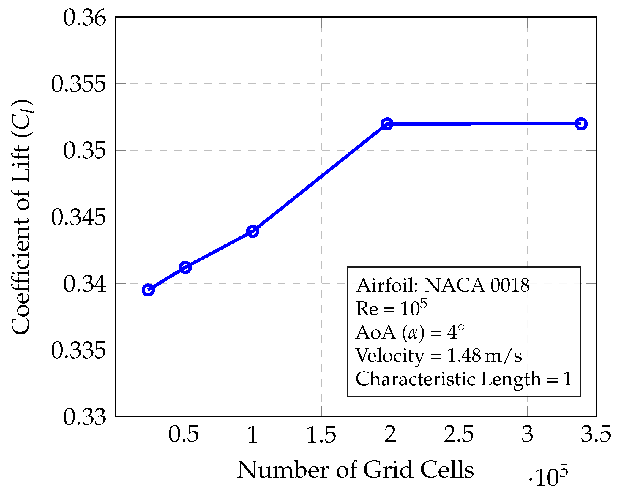
Figure 5.
Mesh Domain
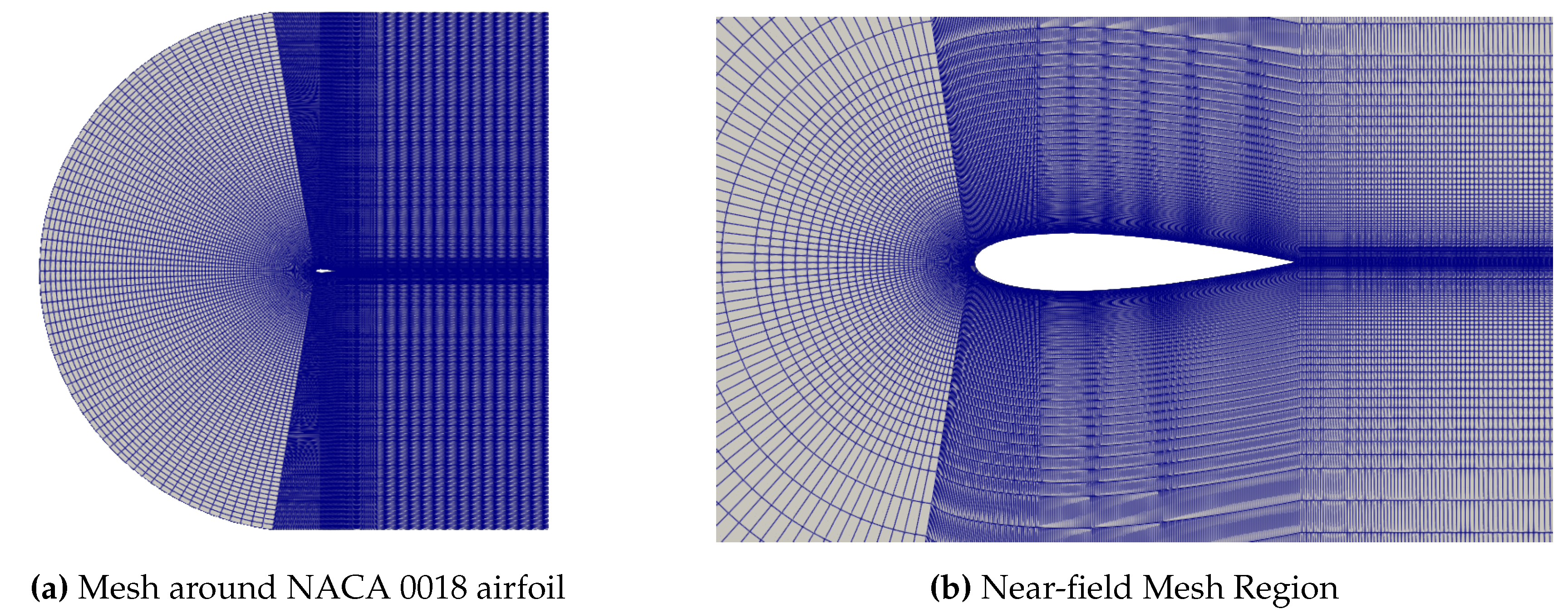
Figure 6.
Software used in the Automation Process

Figure 7.
Approach

Figure 8.
CST Automation using MATLAB®
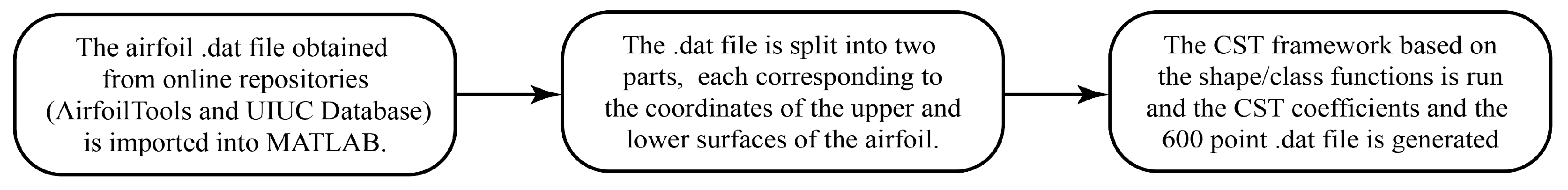
Figure 9.
The data structure of the GitHub Repository
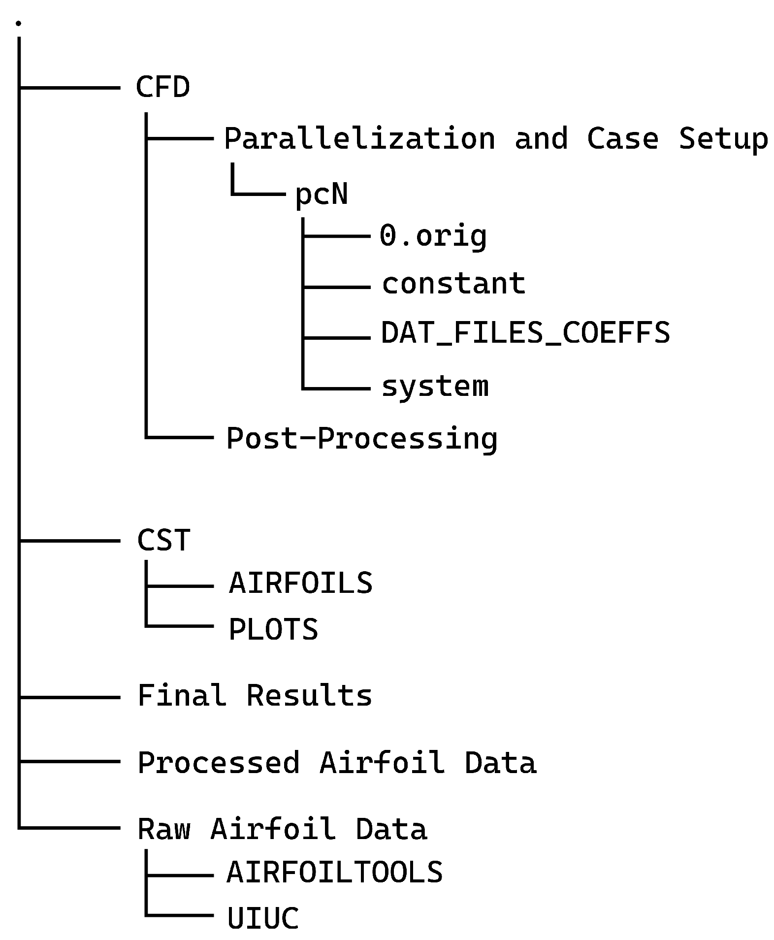
Figure 10.
Aerodynamic characteristics of NACA 0018
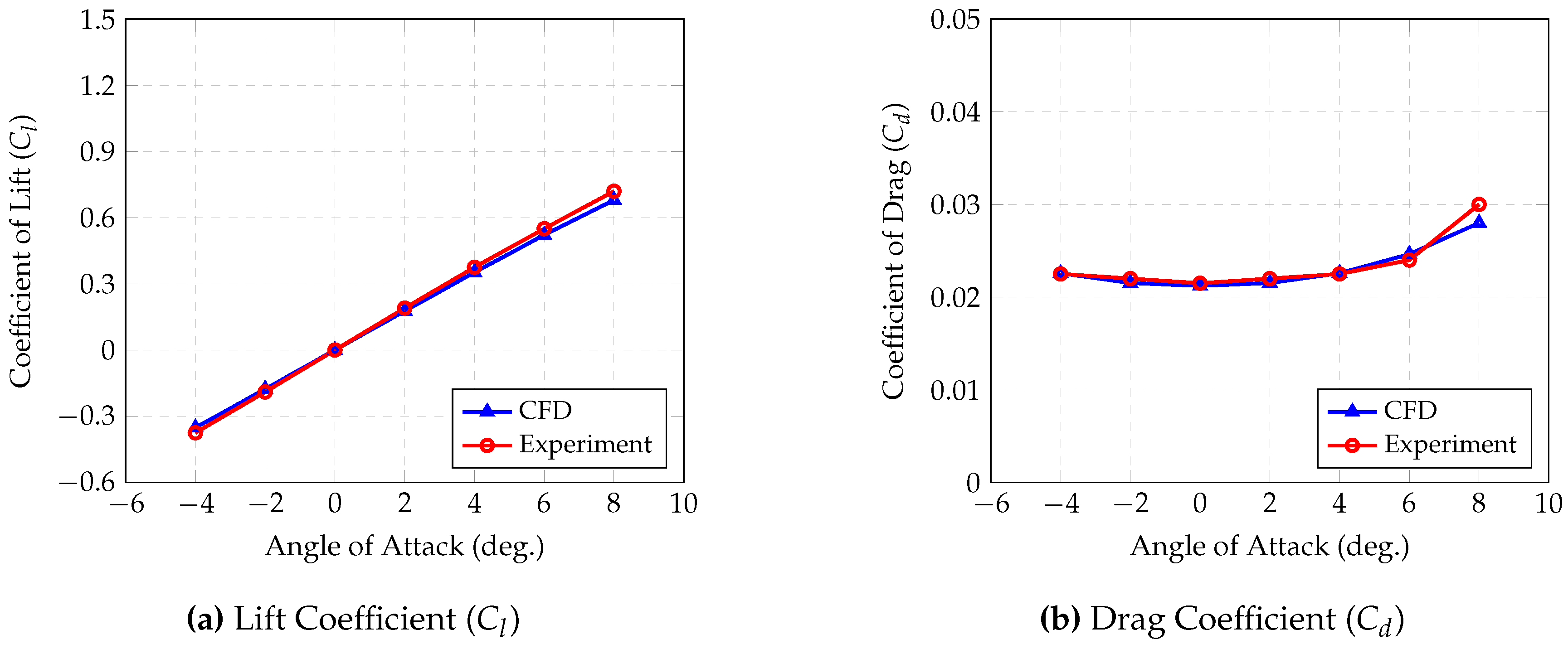
Figure 11.
Aerodynamic characteristics of NACA 2412
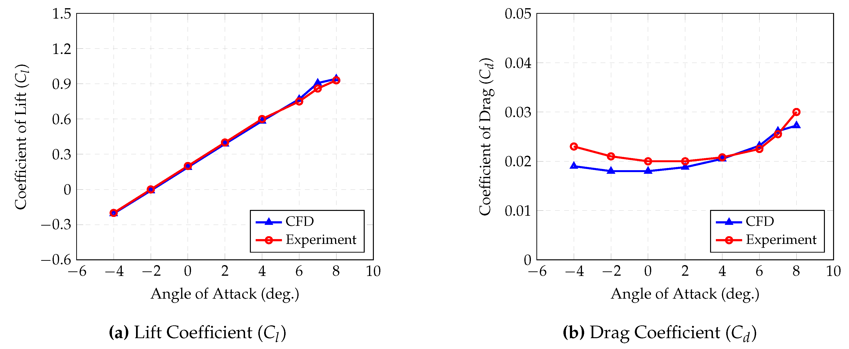

Table 1.
Dataset Format
| Airfoil Filename | AoA () | X1 | X2 | X3 | X4 | X5 | X6 | X7 | X8 |
Disclaimer/Publisher’s Note: The statements, opinions and data contained in all publications are solely those of the individual author(s) and contributor(s) and not of MDPI and/or the editor(s). MDPI and/or the editor(s) disclaim responsibility for any injury to people or property resulting from any ideas, methods, instructions or products referred to in the content. |
© 2024 by the authors. Licensee MDPI, Basel, Switzerland. This article is an open access article distributed under the terms and conditions of the Creative Commons Attribution (CC BY) license (http://creativecommons.org/licenses/by/4.0/).
Copyright: This open access article is published under a Creative Commons CC BY 4.0 license, which permit the free download, distribution, and reuse, provided that the author and preprint are cited in any reuse.


