Submitted:
13 March 2024
Posted:
14 March 2024
You are already at the latest version
Abstract
X-ray Fluorescence Computed Tomography (XFCT) is an emerging non-invasive imaging technique providing molecular-level data, gaining attention for high-resolution imaging. However, increased sensitivity with benchtop X-ray sources raises radiation exposure. Artificial Intelligence (AI), particularly deep learning (DL), has revolutionized medical imaging by delivering high-quality images in the presence of noise. In XFCT, traditional methods rely on complex algorithms for noise reduction, but AI holds promise in addressing high-dose concerns. We present an optimized SCUNet model for noise reduction in low-concentration XRF images. Compared to higher-dose images, our method’s effectiveness is evaluated. While various denoising techniques exist for X-ray and CT, few address to XFCT. The DL model is trained and assessed using the augmented data, focusing on background noise reduction. Image quality is measured using PSNR and SSIM, comparing outcomes with 100% X-ray dose images. Results show the proposed algorithm achieves high-quality images from low-dose and low-contrast agents, with a maximum PSNR of 39.05 and SSIM of 0.86. The model outperforms BM3D, NLM, DnCNN, and SCUNet in both visual inspection and quantitative analysis, particularly in high-noise scenarios. This indicates the potential of AI, specifically the SCUNet model, in significantly improving XFCT imaging by mitigating the trade-off between sensitivity and radiation exposure.
Keywords:
Deep learning
; Artificial Intelligence
; Xray Fluorescence
; XFCT
; AI
; DL
1. Introduction
Over recent decades, there has been exploration into using X-ray fluorescence (XRF) imaging to quantify and determine the biodistribution of labeled contrast agents based on metallic nanoparticles suited for in-vivo preclinical studies with metal nanoparticles [1,2,3,4,5]. For this purpose, various imaging approaches have been proposed with different scanning methodologies and X-ray sources for the excitation characteristic x-ray photons from specific metallic nanoparticles [6]. X-ray fluorescence computed tomography (XFCT) combines XRF with computed tomography (CT). The other researchers measured the distribution of nanoparticles in mice using a monochromatic X-ray source from a synchrotron [5,8,9]. Meanwhile, [6,7] applied conventional X-ray tubes with polychromatic X-rays for biomedical applications, introducing benchtop XFCT imaging (available on the laboratory scale). Cong et al. effectively reconstructed gold nanoparticles by employing a fan-beam X-ray source and parallel single-hole collimation [8]. Deng et al. employed a conventional X-ray tube to observe the distribution of gadolinium nanoparticles within mouse kidneys [7]. However, the primary source of noise is the appearance of Compton-scattered photons in the signal, causing a low signal-to-noise ratio and reduced detection sensitivity. Hence, enhancing image quality involves the essential task of minimizing Compton background noise to solve the mentioned problem. One of the available approaches for extracting XRF signal from Compton-scattered photons is through background-reduction scheme through a spatial filtering algorithm [3,6,9,10,15]. The subtraction process requires consistency in the positioning and posture of the measured object, necessitating two scans (with and without metal nanoparticles) [11,12]. This leads to increasing the radiation dose that causing metabolic abnormalities [1]. Therefore, it is important to move from traditional noise removal methods to the new denoising methods. Recently, deep learning denoising methods have been widely used in the field of biomedical imaging and image processing [13,14]. The convolutional neural network (CNN) architecture can extract features from low to high level, resulting in better identifying and understanding patterns. The methods show a high performance of image-to-image translation issues [15,16]. For example, achieving a high-quality (high-dose) image from a low-dose image by removing the noise [15]. In contrast to the assumption made in non-blind image denoising, which presupposes knowledge of the noise type and level, blind denoising addresses scenarios where either the noise level or the specific noise type, or both, are unknown. Zhang et al. show that a deep model is capable of managing Gaussian denoising across different noise levels [16]. Meanwhile, Chen et al. suggest employing generative adversarial networks (GAN) to create noise from clean images [17]. This generated noise is then used to create paired training data for subsequent training purposes. Guo et al. introduce a convolutional blind denoising network, which incorporates a subnetwork for estimating noise [18]. They further suggest training the model using both a practical noise model and pairs of real-world noisy-clean images. Yue et al. introduce a method using variational inference for blind image denoising [19]. This method unifies both noise estimation and image denoising within a Bayesian framework. Sun and Tappen introduce a non-local deep learning approach that combines the benefits of block matching and 3D filtering (BM3D) and non-local means (NLM) [20]. Lefkimmiatis creates an unrolled network capable of executing non-local processing, leading to enhanced denoising outcomes [21]. Leing et al. show improvement in Peak signal-to-noise ratio (PSNR) performance achieved by a specific method Image Restoration Using Swin Transformer (SwinIR) compared to another method Denoising Convolutional Neural Network (DnCNN) on a benchmark dataset [22]. Liu et al. employ a transformer-based method, shifted window transformer (Swin), as the primary building block. They demonstrate that the Swin model exhibits improved performance when handling images with repetitive structures, verifying the effectiveness of the transformer in enabling non-local modeling capabilities [28]. A different scholar proposed a new blind denoising network architecture named Swin-Conv-UNet (SCUNet), applied it to a real image dataset, and designed it for improved practical usage and enhanced local and non–local modeling abilities [16].
In this study, our objective is to employ blind hybrid deep learning model, SCUNet and enhance its capability for denoising XFCT images. The model is the results of combining the Unet [29] and Swin [16] models, utilizing both local and non-local modeling. These two networks have individually shown a promising denoising performance. The XRF images of the Gadolinium (Gd) contrast agent were generated from high-dose and low-dose to estimate the effect of the radiation dose on background noise by applying the blind hybrid denoising method. The model is created to combine two specific abilities: the local modeling ability of a residual convolutional layer and the non-local modeling ability of a swin transformer block. This combined block is suggested to be used as a fundamental component within the image-to-image translation UNet architecture, potentially enhancing its performance or capabilities. The architecture alone does not suffice for attaining optimal results. Consequently, we incorporated a compound loss function to enhance the network’s performance, specifically addressing the intricacies associated with denoising medical images.
2. Materials and Methods
2.1. Experimental Setup
Gadolinium in varying concentrations, derived from Gadoteric acid (), was utilized as the contrast agent. It was employed on a specifically created water-like phantom for system characterization and on multi–layered in vitro 3D tissue models to simulate in vivo investigations. The Gd calibration sample, 8 mm in diameter, is embedded in small animal water-filled with a maximum diameter of 50 mm and held inside borosilicate glass containers 60 mm high behaving as small animal surrogates. The Gd calibration samples have concentrations ranging from 0–3.1 mg/mL ( 0%, 0.031%, 0.1%, 0.2%, and 0.31% by Gd weight (wt.%) see Figure 1). This figure in the first row shows the varying Gd concentration, and the second row provides an example of the XRF scan in the presence of different Gd concentrations.
We employed attenuation images from Cone Beam Computed Tomography (CBCT) to correct for attenuation in the XRF images. The data used in this study consists of XRF images generated from Gd-embedded target phantoms. The XRF data was acquired using Cone-beam polychromatic X-rays generated from a tungsten-target microfocus X-ray tube (Oxford Nova 600). The incident polychromatic X-rays with 90 kVp, a maximum beam current of 0.9 mA, 0.3 mm Copper filtration, and a diameter focal size of 14-20 m were used as an excitation source for both CBCT and XFCT imaging systems. The distance from the source-to-isocenter is 40.5 cm and the source-to-detector of 55.7 cm. Figure 2 shows the experimental setup of the benchtop XFCT imaging system. 30 images were captured with an angular spacing of 12 degrees between each image, and approximately 6 seconds were allocated for the exposure time of each image.
In the existing XFCT configuration, the Timepix3 HPCD (with pixel dimention of 55 µm × 55 µm , an active detection area of approximately 14 mm × 14 mm, a 1 mm CdTe sensor thickness, and an energy resolution of around 4 to 6 keV FWHM Gd XRF energies, Minipix TPX3, Advacam) was exposed to radiation using a single-pinhole arrangement with a circular aperture. This setup also involved the use of Minipix TPX3 and Advacam. The pinhole collimator constructed from lead, had an aperture diameter of 0.4 mm and a thickness of 1.5 mm. To conduct full-field scanning within a large CT system that had specific geometric constraints, adjustments were made to the distances between the X-ray source and the isocenter 14 cm. Distances of 5.5 cm from the Xray source to the isocenter were set, with a pinhole to detector distance of 1.5 cm. A sparse-view image acquisition strategy using compressed sensing was employed to reduce radiation exposure. This strategy involved taking only 10 angular projections within a 360° scan, each with an exposure time of 150 seconds per projection.
2.2. Deep Blind Image Denoising Model
2.2.1. Dataset
To estimate the effect of radiation dose on background noise, various levels of noisy images are generated (low to high dose). The noisy datasets are generated by reducing the raw data photons (100% photons- high dose images-) by the factor of 25%, 50%, and 75% (low dose images). Additionally, for each image, three bin widths corresponding to 0.05 KeV, 0.1 KeV, and 0.5 KeV are used. Herein, smaller bin widths correspond to a finer sampling grid, however, with reduced number of entries per XRF signal bin. Furthermore, To address the limitation posed by the small dataset, we employed a data augmentation technique known as rotation. Data augmentation involves creating additional training samples by applying various transformations to the existing data. In our case, rotation augmentation was chosen to enhance the diversity of the dataset. Rotation augmentation entails rotating the original images by certain angles to generate new perspectives and variations. We specifically chose rotation angles of 90, 180, and 270 degrees for several reasons. Firstly, these angles represent orthogonal transformations, allowing the model to learn diverse features and patterns that may be present in different orientations. Secondly, these angles align with common geometric transformations, capturing potential variations that could be encountered in real-world scenarios. The SCUNet training pipeline involves utilizing denoised images as targets and noisy images as input for the model. Through this approach, the sample size was effectively increased by approximately tenfold. Within the training pipeline, a hold-out strategy was implemented, allocating 20% of the samples for testing in each category and utilizing the remaining 80% for training purposes. The DL model is trained using augmented data and evaluated for background noise reduction via the proposed denoising approach.
2.2.2. Proposed Model
In this study, a blind denoising method was employed to effectively remove noise present in the images. The blind image denoising, where the process of obtaining an estimated clean image involves solving a specific Maximum A Posteriori (MAP) problem using an optimization algorithm. This method aims to derive the best estimation of the original (clean) image X from a noisy image by employing the following optimization technique:
Where D(x,y) represents the data fidelity component, ’P(x)’ represent the prior term, and is the trade-off parameter [16]. At this point, it becomes evident that the crux of addressing blind denoising is twofold: modeling the degradation process of a noisy image and designing the image prior for a clean image. Conceptually, by regarding the deep model as a condensed unrolled inference of Equation 1, the overarching objective of deep blind denoising typically involves tackling the following bi-level optimization problem [30,31]. The effectiveness of the deep blind learning model is largely dependent on its network architecture and the quality of the training data. The presence of noisy images in the training dataset significantly influences the model’s understanding of the degradation process. Improvements in the network architecture and the inclusion of clean images within the training dataset play a crucial role in shaping this understanding. Improving the quality of clean data is achievable, but additional investigation is necessary to enhance and develop network architecture.
The network architecture of SCUNet model is shown in Figure 3. The core concept behind SCUNet involves merging the complementary network architecture designs from dilated-residual U-Net (DRUNet) and SwinIR. Specifically, SCUNet incorporates novel swin-conv (SC) blocks into a UNet backbone [29]. In accordance with DRUNet [32], SCUNet’s UNet backbone consists of four scales, each featuring a residual connection between 2 × 2 strided convolution (SConv) based downscaling and 2 × 2 transposed convolution (TConv) based upscaling. The channel counts in each layer vary from 64 in the first scale to 512 in the fourth scale. A key distinction between SCUNet and DRUNet lies in the adoption of four SC blocks, as opposed to four residual convolution blocks, in each scale of the downscaling and upscaling process. The images of the XRF photons including Compton scattered photons were inputted into the network with a size of 256 x 256 pixels, and the output images were all the same size. Transformer layer SwinIR model consists of shallow feature extraction, deep feature extraction and high-quality image reconstruction. We treat each patch as a token and 2 x 2 strided convolution with stride 2. The UNet backbone of our model has four scales, each of which has a residual connection between 2 x 2 SConv based downscaling and TConv based upscaling. The number of channels in each layer from the first scale to the fourth scale are 64, 128, 256 ,and 512, respectively.
The dashed line in Figure 3 illustrates an SC block that combines a swin transformer (SwinT) block [28] with a residual convolutional (RConv) block [34,35] through two 1 × 1 convolutions, split and concatenation operations, and a residual connection. Specifically, for an input feature tensor, it undergoes an initial 1 × 1 convolution. Following this, the tensor is evenly divided into two feature map groups, namely X1 and X2. This entire process can be expressed as follows:
Subsequently, X1 and X2 are individually inputted into a SwinT block and an RConv block, leading to:
Finally, Y1 and Y2 are concatenated to form the input of a 1 × 1 convolution, which establishes a residual connection with the initial input tensor, X. Consequently, the ultimate output of the SC block is expressed as:
Our proposed SCUNet exhibits several advantages attributed to its innovative module designs. Firstly, the SC block integrates the local modeling capability of the RConv block with the non-local modeling ability of the SwinT block. Secondly, the local and non-local modeling capabilities of SCUNet are further enhanced through the incorporation of a multiscale UNet. Thirdly, the 1 × 1 convolution plays a crucial role in effectively and efficiently facilitating information fusion between the SwinT block and the RConv block. Fourthly, the split and concatenation operations serve as a form of group convolution with two groups, contributing to the reduction of computational complexity and the number of parameters. The parameters are optimized by minimizing the L1 loss with Adam optimizer [36]. The learning rate starts from and and decays by a factor of 0.9 for each iteration for 40 epochs. The batch size is set to 2. We first train the model with noise level 25 and then finetune the model for other noise levels. All experiments are implemented by PyTorch 2.0.1. It takes about 20 hours to train a denoising model on NVIDIA GTX 1080.
It is noteworthy that SCUNet operates as a hybrid CNNs–Transformer network, integrating features from both architectures. Similar approaches exist in the literature, where researchers have explored the combination of CNNs and Transformers for effective network architecture design. It is significant to highlight the distinctions between our proposed SCUNet and two recent works, namely Uformer [37] and Swin-Unet [38]. Firstly, the motivation behind each approach differs significantly. SCUNet is inspired by the observation that state-of-the-art denoising methods, DRUNet [32] and SwinIR [22], leverage distinct network architecture designs. As a result, SCUNet seeks to integrate the complementary features of DRUNet and SwinIR. Conversely, Uformer and Swin-UNet aim to merge transformer variants with UNet, serving a different motivation.
Secondly, the primary building blocks employed in each model are distinct. SCUNet incorporates a novel swin-conv block, which int egrates the local modeling capability of the residual convolutional layer [34] with the non-local modeling ability of the swin transformer block [28] through 1 × 1 convolution, split, and concatenation operations. In contrast, Uformer adopts a novel transformer block by combining depth-wise convolution layers [39], while Swin-UNet utilizes the swin transformer block as its primary building block.
3. Results and Discussion
As outlined in Section 2.2, enhancing the performance of the deep blind denoising model relies on the optimization of both the network architecture and the training data. We evaluate the performance of our model qualitatively and quantitatively and compere it with other deep and non-deep learning methods.
To achieve optimal denoising results, we initiated our model training by utilizing the official pre-trained weights of SCUNet. Subsequently, we fine-tuned the model on our specific dataset, enhancing its adaptability to our unique denoising requirements. During this training process, a compound loss function was employed to synergistically improve the overall performance of the model. Figure 4 shows examples of images in our dataset with varying noise levels and bin widths. In the first row, we present our original data with 100% of the initial number of photons. Subsequently, we reduce the number of photons by a factor of 25% in each following row, simultaneously increasing the sampling rate to 0.05, 0.1, and 0.5. In this figure the highest quality image is the image with noise-level of 0% and maximum bin width (BW) of 0.5 (first row and second column), and the lowest quality image is the one with 75% noise-level and bin widths of 0.5.
Figure 5, Figure 6, and Figure 7 showcase the predicted denoising qualitative results for various methods at noise levels of 25%, 50%, and 75%, respectively. These tables compare state-of-the-art techniques with our proposed model on our dataset. In the second row of each table, the results of the BM3D method are presented. BM3D, a 3D block-matching algorithm primarily used for noise reduction in images, is an extension of the NLM methodology [40]. The third row displays the outcomes of the NLM method, involving the calculation of a mean value for all pixels in the images, with weights assigned based on the similarity of each pixel to the target pixel [41]. Moving to the fourth row, we observe the results of the DnCNN [42]. This method aims to recover the clean image x from the noisy image , assuming v is Additive White Gaussian Noise (AWGN). The network can handle Gaussian denoising with an unknown noise level. In general, image denoising methods can be categorized into two major groups: model-based methods, like BM3D, which are flexible in handling denoising problems with various noise levels but are time-consuming and require complex priors, and discriminative learning-based methods, like DnCNN, developed to overcome these drawbacks. In the fifth row, we present the results of blind image denoising via the SCUNet method [33]. While existing methods rely on simple noise assumptions, such as AWGN, the SCUNet method is designed to address all unknown noise types that remained unsolved in previous methods. The last row showcases the results of our method, which extends the performance of the SCUNet method. The qualitative results of the proposed model consistently yield superior visual outcomes across all different bin widths. While BM3D exhibits better visual results, it tends to produce smoother images, consequently removing important details. In contrast, the proposed method generates images that closely resemble the original (0% noise) image. DnCNN, on the other hand, produces results that closely match images at the same noise level.
Figure 8 presents the comparison results of predicted denoising for various methods at a 75% noise level, with reference to the 0% noise condition. The findings indicate that our proposed model exhibits significantly improved visual results, closely resembling the original image even under high and low sampling rates.
In addition to the qualitative comparison of different methods, we present the quantitative results for noise levels of 25%, 50%, and 75%, based on two measurement factors: PSNR and SSIM, respectively, in Table 1 and Table 2. The compared methods include BM3D, NLM, DnCNN, and SCUNet. It can be observed that our proposed method achieved significantly better PSNR and SSIM results than other methods for the highest noise levels. Except in comparison with DnCNN, which has higher PSNR and SSIM for the two noise levels of 25% and 50%, our method outperformed the others in terms of PSNR and SSIM.However we are believe that the good results of DnCNN is because of its match with the same noise level. We can see from the results of both tables that the SCUNet method has significantly lower results at all different noise levels compared to our proposed model.
4. Conclusions
In this study, we refined the SCUNet deep learning model to enhance its applicability for noise reduction in XFCT images. To optimize the application to our image data, we implemented a compound loss function [43] aimed at capturing shape-aware weight maps, addressing specific challenges posed by medical images within the SCUNet architecture. Our approach, as indicated in Table 1 and Table 2 demonstrated improved outcomes, showcasing the effectiveness of the compound loss function [43].
To assess the efficacy of our approach, we conducted comparative analyses against four existing models BM3D, NLM, DnCNN, and the original SCUNet. These comparisons could demonstrate the efficiency of our blind deep learning model in eliminating all types of noise, including unknown noise, alongside known image noise such as AGN. Our overarching goal is to produce clean XFCT images from concurrent noisy images, corresponding to low-dose image acquisition, in order to enable low-dose XFCT imaging.
To facilitate our research, we curated a dataset comprising reconstructed images derived from sparse-view benchtop XFCT images. The deep learning model underwent training and evaluation, utilizing two key metrics of PSNR and SSIM. The results on experimental data provides insights into the effectiveness of our proposed method for denoising Gaussian noise and suggests potential practicality of the trained deep blind model in handling real noisy images.
Analysis of the results, as illustrated in Figure 8, shows robust performance of our model across varying levels of noise and low-dose photon scenarios, transcending three different bin widths. Conversely, other methods exhibited performance dependency on bin widths values and noise levels. Further insights from Figure 5, Figure 6, and Figure 7 showcased the output of all models under different noise conditions of 25%, 50%, and 75%, respectively.
Quantitative assessments of noise removal demonstrated better performance of our proposed model compared to BM3D, NLM, and the original SCUNet. Our method demonstrated notable proficiency in handling images with high noise and sparse sampling, surpassing other studied methods, including SCUNet. Finally, our method achieved a maximum PSNR of 39.05 and SSIM of 0.86, indicating the improved performance of our model.
Author Contributions
N.M, M.R developed methodology. M.F, K.K, and C.H conceived the project and designed experiments. M.F, K.K acquired data. N.M analyzed and interpreted data. N.M, M.R, K.K, M.F wrote, reviewed, or revised the manuscript. AA.I provided the results of the literature methods. C.H supervised the study. All authors read and approved the final manuscript.
Funding
This research received no funding.
Data Availability Statement
The raw data supporting the conclusion of this article will be made available by the authors, without undue reservation.
Conflicts of Interest
The authors declare that the research was conducted in the absence of any commercial or financial relationships that could be construed as a potential conflict of interest.
Abbreviations
The following abbreviations are used in this manuscript:
| XFCT | X-ray fluorescence computed tomography |
| XRF | X-ray fluorescence |
| AI | Artificial Intelligence |
| DL | Deep Learning |
| SCUNet | Swin-Conv-UNet |
| CT | Computed Tomography |
| PSNR | Peak signal-to-noise ratio |
| SSIM | Structural Similarity Index |
| BM3D | Block-Matching and 3D filtering |
| NLM | Non-local means |
| DnCNN | Denoising Convolutional Neural Network |
| CNN | convolutional neural network |
| GAN | generative adversarial networks |
| Gd | Gadolinium |
| wt | Weight |
| Swin | Shifted window Transformer |
| KeV | Kilo electron volt |
| mA | miliampere |
| CBCT | Cone Beam Computed Tomography |
| MAP | Maximum A Posteriori |
| DRUNet | Dilated-Residual U-Net |
| SwinIR | Image Restoration Using Swin Transformer |
| SConv | Strided Convolution |
| TConv | Transposed Convolution |
| RConv | Residual Convolutional |
| SwinT | Swin Transformer |
| BW | bin width |
| AWGN | Additive White Gaussian Noise |
References
- Feng, P.; Luo, Y.; Zhao, R.; Huang, P.; Li, Y.; He, P.; Tang, B.; Zhao, X. Reduction of Compton background noise for X-ray fluorescence computed tomography with deep learning. Photonics 2022, 9, 108. [Google Scholar] [CrossRef]
- Zhang, S.; Li, L.; Chen, J.; Chen, Z.; Zhang, W.; Lu, H. Quantitative imaging of Gd nanoparticles in mice using benchtop cone-beam X-ray fluorescence computed tomography system. International journal of molecular sciences 2019, 20, 2315. [Google Scholar] [CrossRef] [PubMed]
- Manohar, N.; Reynoso, F.J.; Diagaradjane, P.; Krishnan, S.; Cho, S.H. Quantitative imaging of gold nanoparticle distribution in a tumor-bearing mouse using benchtop x-ray fluorescence computed tomography. Scientific reports 2016, 6, 22079. [Google Scholar] [CrossRef] [PubMed]
- Larsson, J.C.; Vogt, C.; Vågberg, W.; Toprak, M.S.; Dzieran, J.; Arsenian-Henriksson, M.; Hertz, H.M. High-spatial-resolution x-ray fluorescence tomography with spectrally matched nanoparticles. Physics in Medicine & Biology 2018, 63, 164001. [Google Scholar]
- Takeda, T.; Yu, Q.; Yashiro, T.; Zeniya, T.; Wu, J.; Hasegawa, Y.; Hyodo, K.; Yuasa, T.; Dilmanian, F.; Akatsuka, T.; others. Iodine imaging in thyroid by fluorescent X-ray CT with 0.05 mm spatial resolution. Nuclear Instruments and Methods in Physics Research Section A: Accelerators, Spectrometers, Detectors and Associated Equipment 2001, 467, 1318–1321. [Google Scholar] [CrossRef]
- Cheong, S.K.; Jones, B.L.; Siddiqi, A.K.; Liu, F.; Manohar, N.; Cho, S.H. X-ray fluorescence computed tomography (XFCT) imaging of gold nanoparticle-loaded objects using 110 kVp x-rays. Physics in Medicine & Biology 2010, 55, 647. [Google Scholar]
- Deng, L.; Ahmed, M.F.; Jayarathna, S.; Feng, P.; Wei, B.; Cho, S.H. A detector’s eye view (DEV)-based OSEM algorithm for benchtop X-ray fluorescence computed tomography (XFCT) image reconstruction. Physics in Medicine & Biology 2019, 64, 08NT02. [Google Scholar]
- Cong, W.; Shen, H.; Cao, G.; Liu, H.; Wang, G. X-ray fluorescence tomographic system design and image reconstruction. Journal of X-ray science and technology 2013, 21, 1–8. [Google Scholar] [CrossRef] [PubMed]
- Jones, B.L.; Manohar, N.; Reynoso, F.; Karellas, A.; Cho, S.H. Experimental demonstration of benchtop x-ray fluorescence computed tomography (XFCT) of gold nanoparticle-loaded objects using lead-and tin-filtered polychromatic cone-beams. Physics in Medicine & Biology 2012, 57, N457. [Google Scholar]
- Ahmad, M.; Bazalova-Carter, M.; Fahrig, R.; Xing, L. Optimized detector angular configuration increases the sensitivity of x-ray fluorescence computed tomography (XFCT). IEEE transactions on medical imaging 2014, 34, 1140–1147. [Google Scholar] [CrossRef] [PubMed]
- Jung, S.; Sung, W.; Ye, S.J. Pinhole X-ray fluorescence imaging of gadolinium and gold nanoparticles using polychromatic X-rays: a Monte Carlo study. International Journal of Nanomedicine 2017, 5805–5817. [Google Scholar] [CrossRef] [PubMed]
- Jung, S.; Kim, T.; Lee, W.; Kim, H.; Kim, H.S.; Im, H.J.; Ye, S.J. Dynamic in vivo X-ray fluorescence imaging of gold in living mice exposed to gold nanoparticles. IEEE transactions on medical imaging 2019, 39, 526–533. [Google Scholar] [CrossRef] [PubMed]
- LeCun, Y.; Bengio, Y.; Hinton, G. Deep learning. nature 2015, 521, 436–444. [Google Scholar] [CrossRef] [PubMed]
- Szegedy, C.; Liu, W.; Jia, Y.; Sermanet, P.; Reed, S.; Anguelov, D.; Erhan, D.; Vanhoucke, V.; Rabinovich, A. Going deeper with convolutions. In Proceedings of the IEEE conference on computer vision and pattern recognition, 2015; pp. 1–9. [Google Scholar]
- Chen, H.; Zhang, Y.; Kalra, M.K.; Lin, F.; Chen, Y.; Liao, P.; Zhou, J.; Wang, G. Low-dose CT with a residual encoder-decoder convolutional neural network. IEEE transactions on medical imaging 2017, 36, 2524–2535. [Google Scholar] [CrossRef] [PubMed]
- Zhang, K.; Zuo, W.; Chen, Y.; Meng, D.; Zhang, L. Beyond a gaussian denoiser: Residual learning of deep cnn for image denoising. IEEE transactions on image processing 2017, 26, 3142–3155. [Google Scholar] [CrossRef] [PubMed]
- Chen, J.; Chen, J.; Chao, H.; Yang, M. Image blind denoising with generative adversarial network based noise modeling. In Proceedings of the IEEE conference on computer vision and pattern recognition, 2018; pp. 3155–3164. [Google Scholar]
- Guo, S.; Yan, Z.; Zhang, K.; Zuo, W.; Zhang, L. Toward convolutional blind denoising of real photographs. In Proceedings of the IEEE/CVF conference on computer vision and pattern recognition, 2019; pp. 1712–1722. [Google Scholar]
- Krull, A.; Buchholz, T.O.; Jug, F. Noise2void-learning denoising from single noisy images. In Proceedings of the IEEE/CVF conference on computer vision and pattern recognition, 2019; pp. 2129–2137. [Google Scholar]
- Sun, J.; Tappen, M.F. Learning non-local range Markov random field for image restoration. CVPR 2011. IEEE; 2011; pp. 2745–2752.
- Lefkimmiatis, S. Non-local color image denoising with convolutional neural networks. In Proceedings of the IEEE conference on computer vision and pattern recognition, 2017; pp. 3587–3596. [Google Scholar]
- Liang, J.; Cao, J.; Sun, G.; Zhang, K.; Van Gool, L.; Timofte, R. Swinir: Image restoration using swin transformer. In Proceedings of the IEEE/CVF international conference on computer vision, 2021; pp. 1833–1844. [Google Scholar]
Figure 1.
The Gd calibration samples have concentrations ranging from 0 – 3.1 mg/mL.
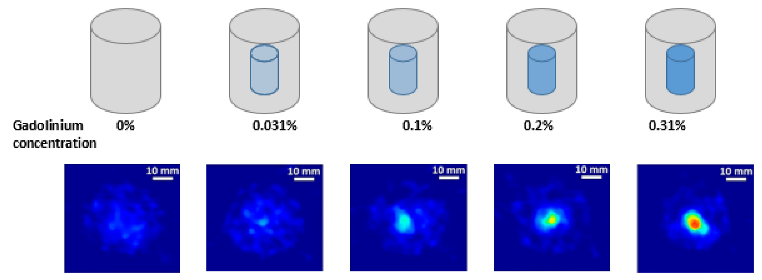
Figure 2.
The setup of the experimental benchtop XFCT system.
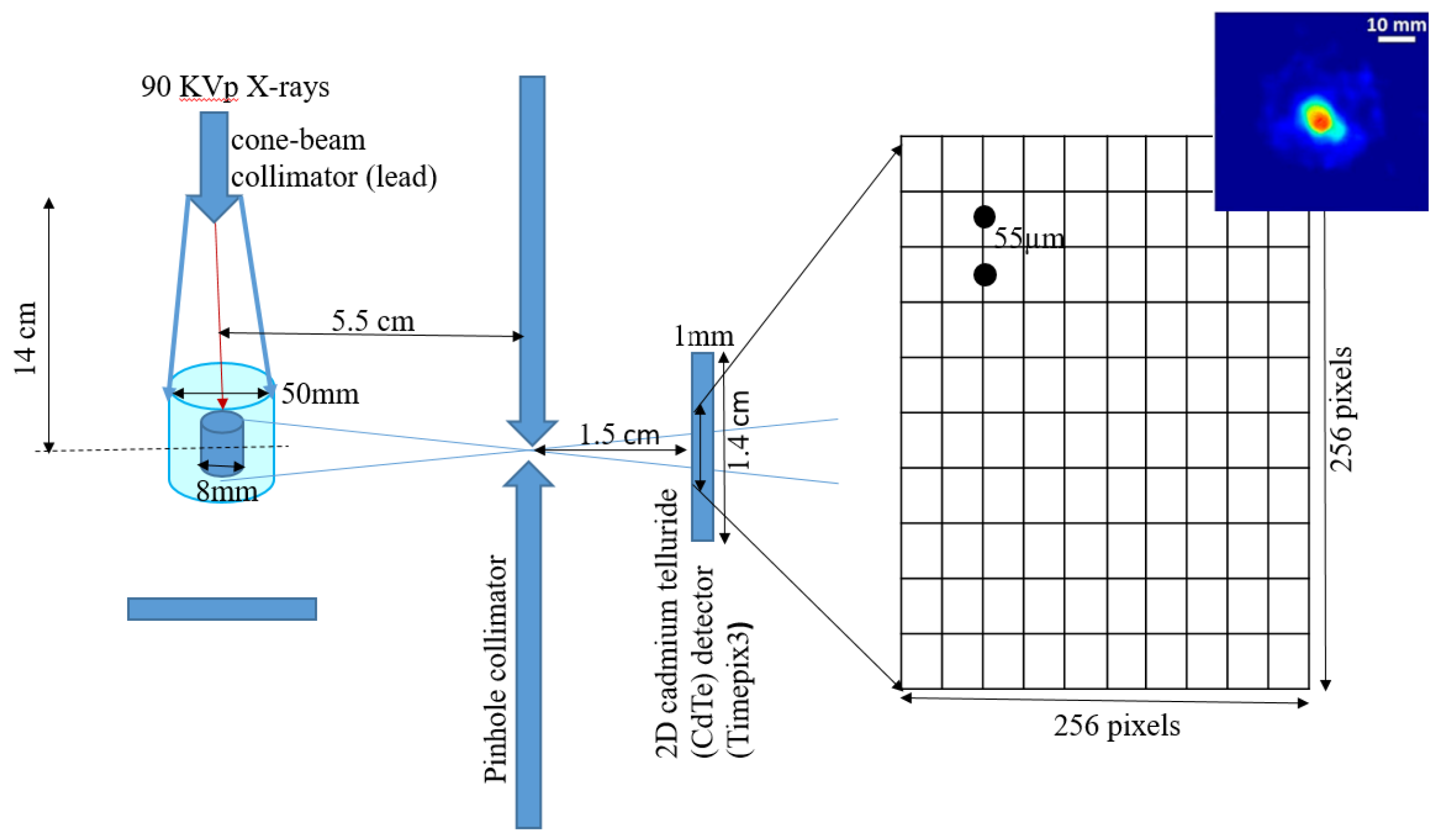
Figure 3.
The architecture of the proposed method and SCUNet ([33]) denoising network.
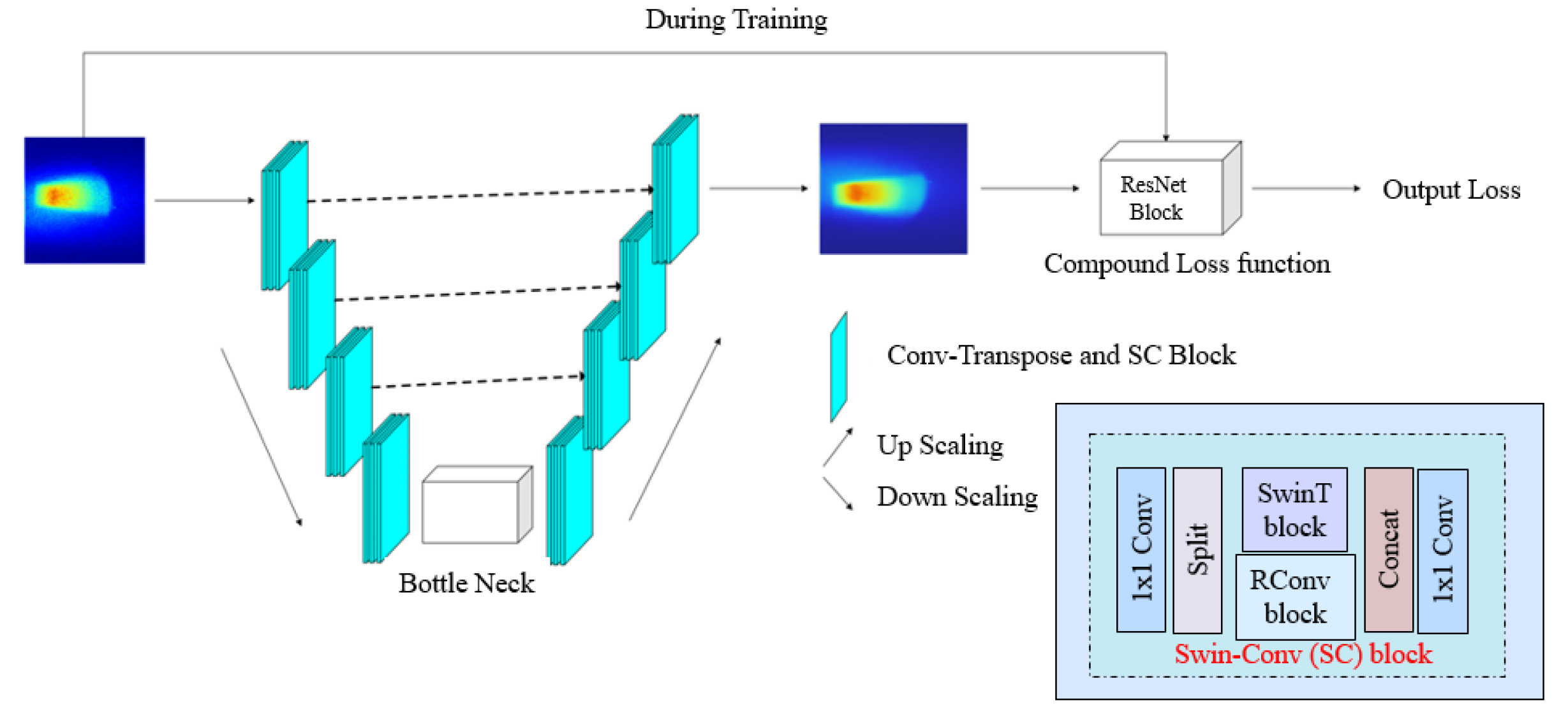
Figure 4.
Data examples from our dataset include four different noise levels and three different bin widths (BW-0.005, BW-0.1, BW-0.5)
Figure 4.
Data examples from our dataset include four different noise levels and three different bin widths (BW-0.005, BW-0.1, BW-0.5)
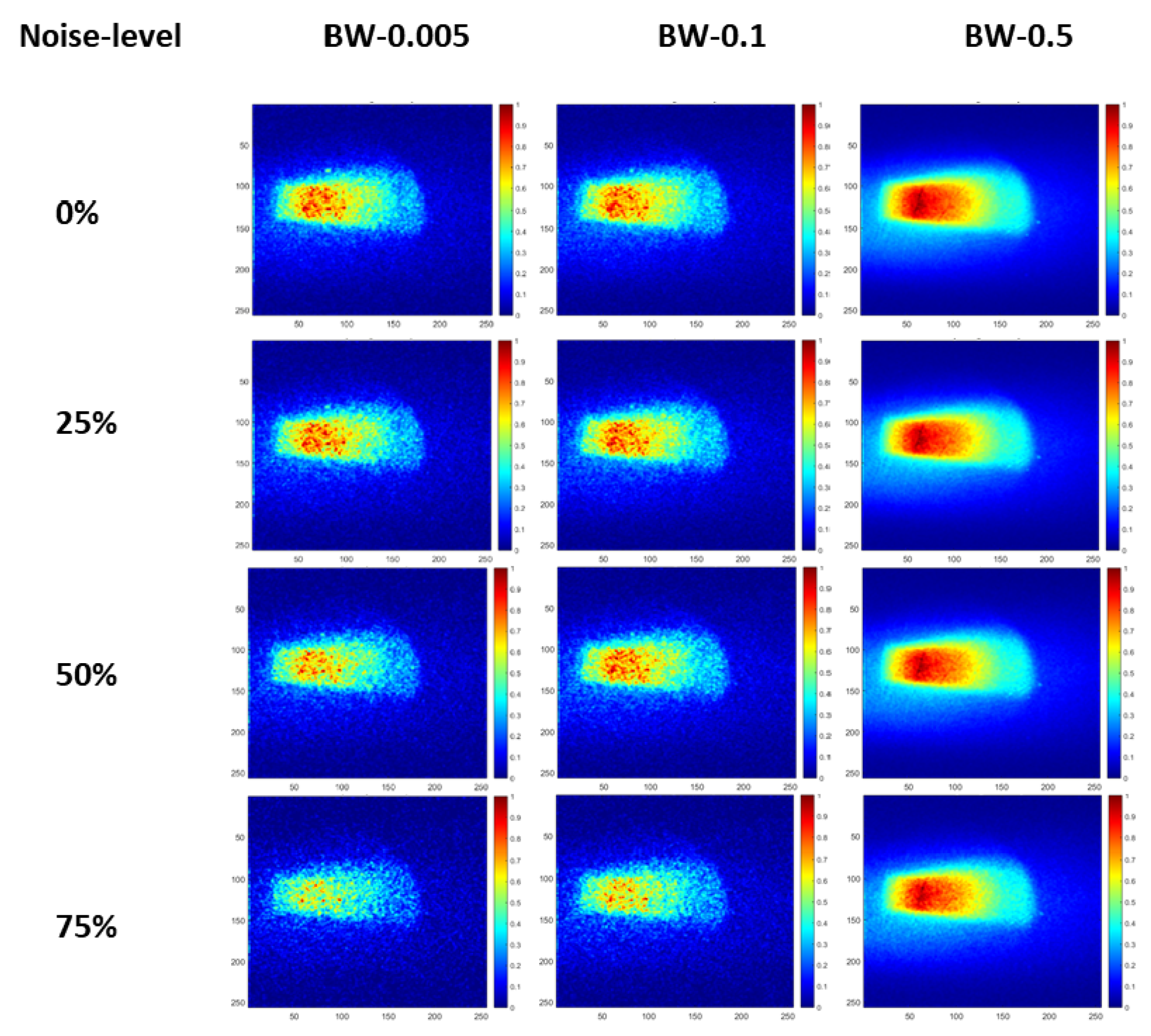
Figure 5.
Visually comparison predicted results of our method with other methods (noise-level 25%)
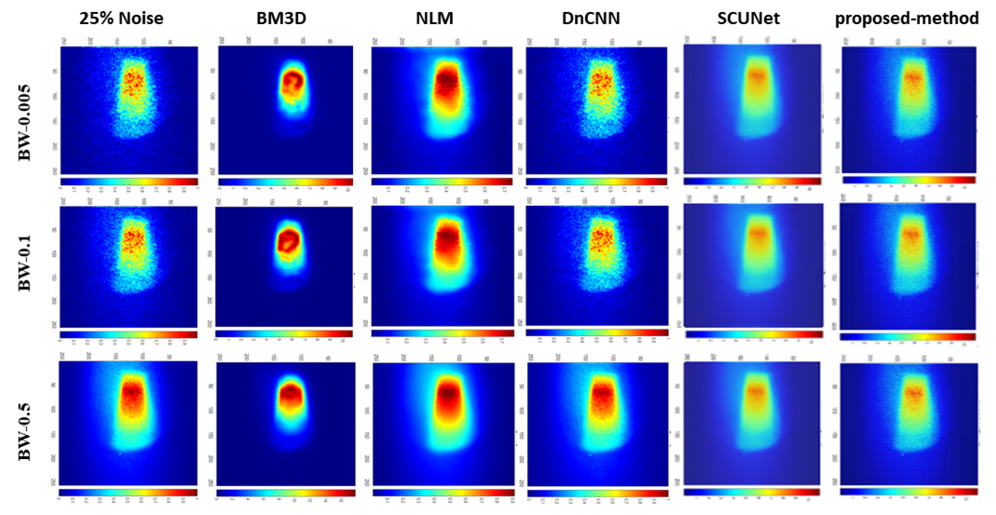
Figure 6.
Visually comparison predicted results of our method with other methods (noise-level 50%)
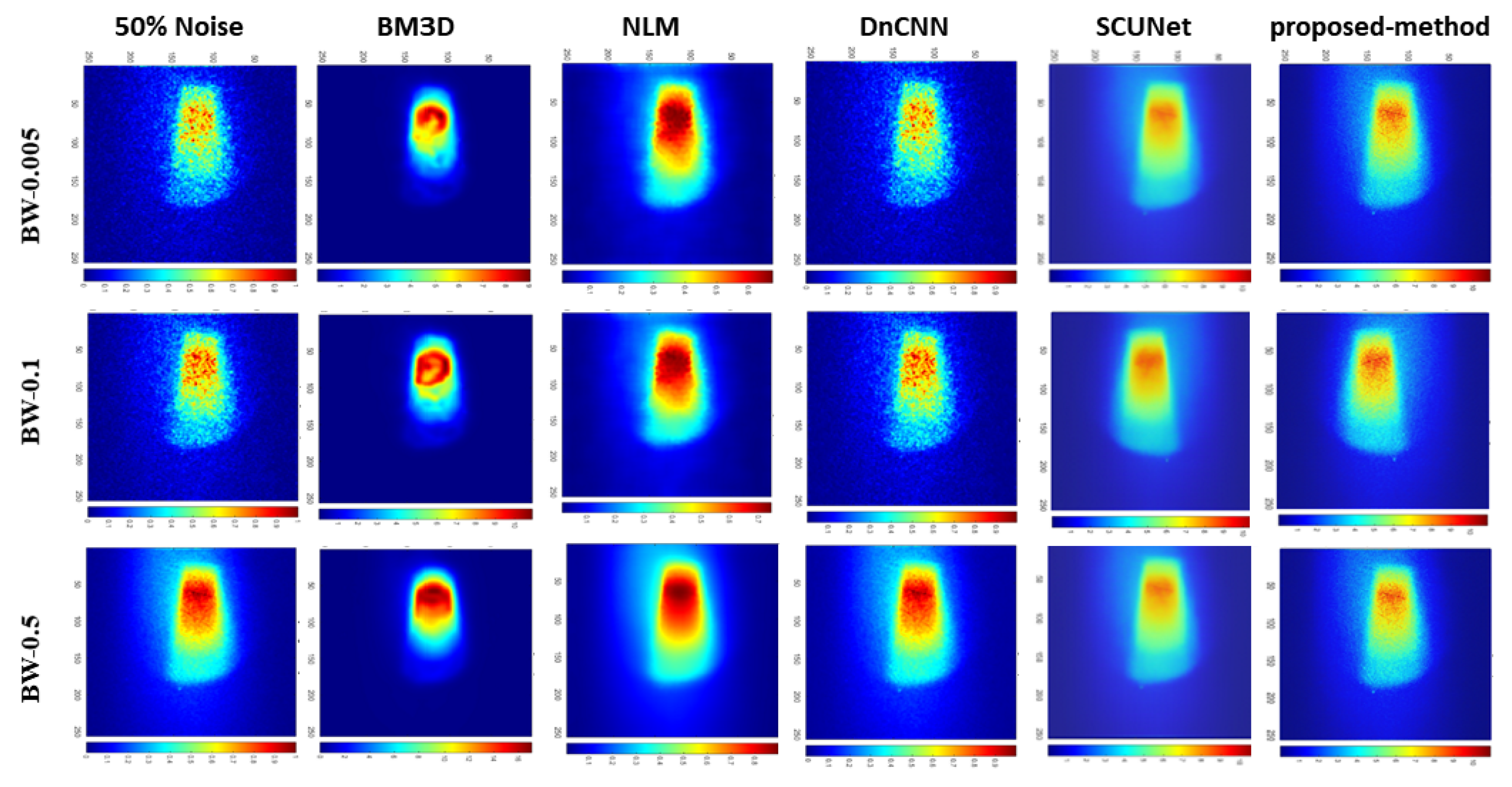
Figure 7.
Visually comparison predicted results of our method with other methods (noise-level 75%)
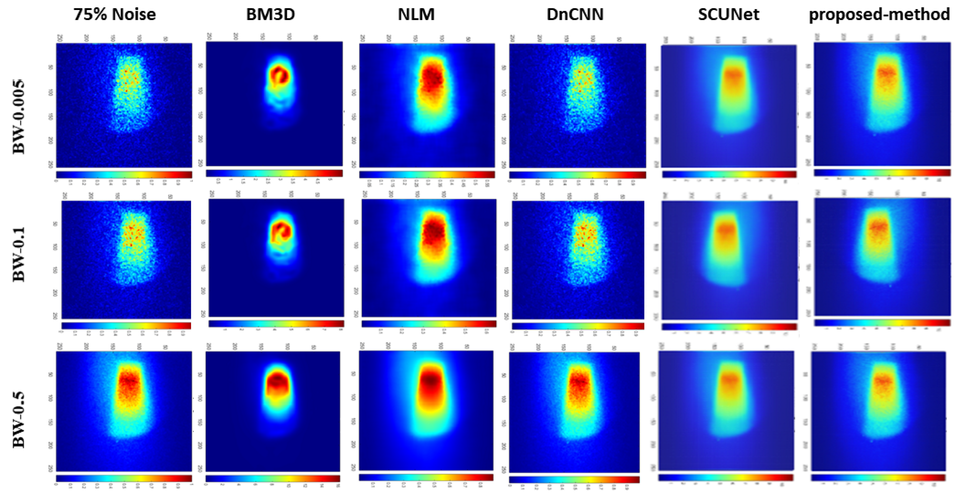
Figure 8.
Visually comparison predicted results of our method with original image(0%Noise)
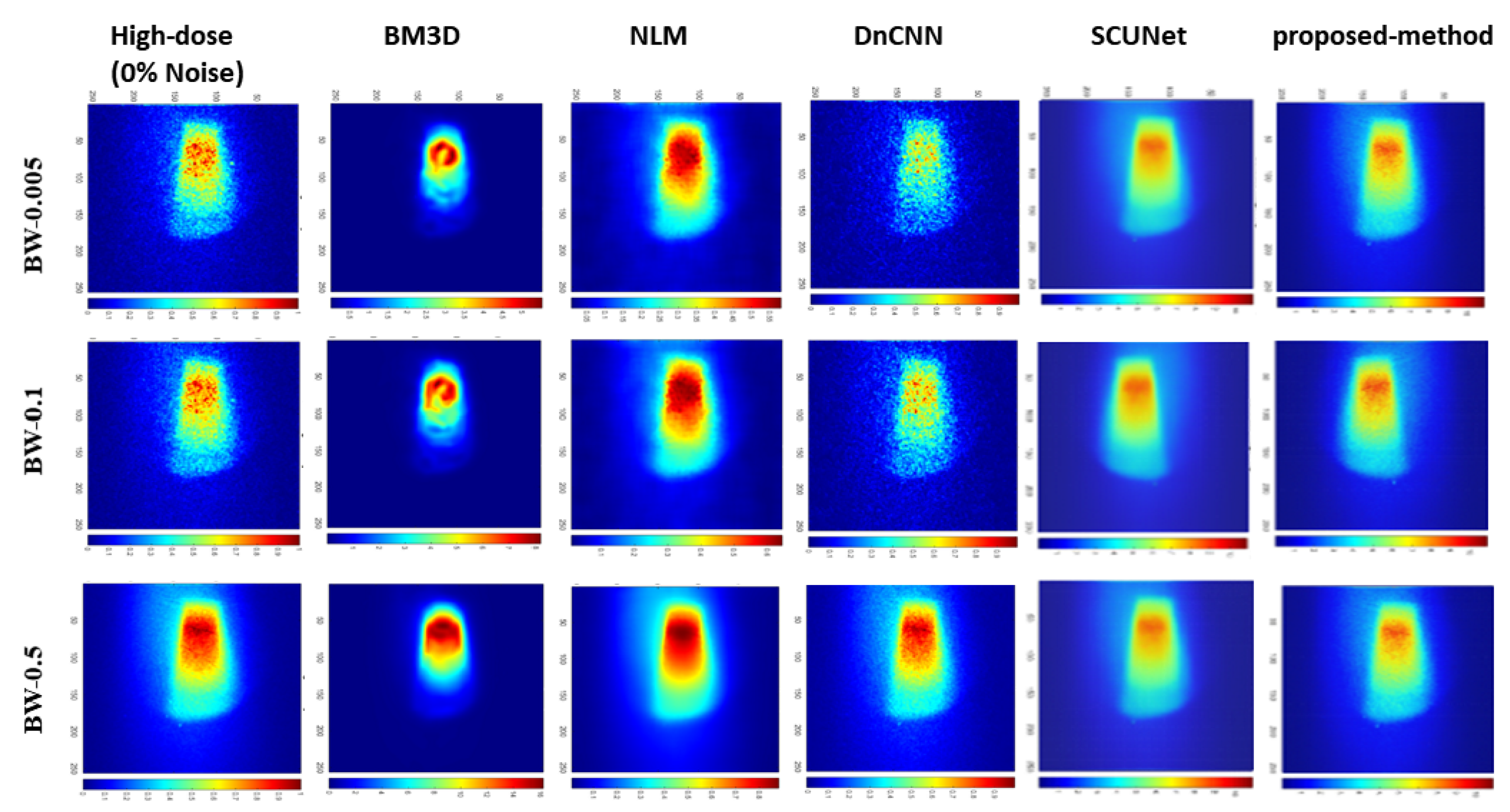

Table 1.
The quantitative results of denoising methods based on PSNR.
| Bin widths | Noise-level | BM3D | NLM | DnCNN | SCUNet | Proposed model |
|---|---|---|---|---|---|---|
| BW-0.05 | 25% | 13.93 | 27.92 | 36.82 | 22.77 | 29.68 |
| 50% | 13.91 | 25.16 | 31.07 | 24.51 | 26.97 | |
| 75% | 13.89 | 24.58 | 24.75 | 25.29 | 31.44 | |
| BW-0.1 | 25% | 13.70 | 32.42 | 38.88 | 22.87 | 35.48 |
| 50% | 13.70 | 28.19 | 34.50 | 27.82 | 29.06 | |
| 75% | 13.67 | 27.71 | 27.75 | 26.77 | 29.33 | |
| BW-0.5 | 25% | 11.76 | 39.94 | 49.35 | 22.54 | 31.81 |
| 50% | 11.75 | 38.77 | 43.66 | 22.74 | 32.67 | |
| 75% | 11.75 | 36.75 | 38.40 | 25.58 | 39.05 |
Table 2.
The quantitative results of denoising methods based on SSIM.
| Bin Widths | Noise-level | BM3D | NLM | DnCNN | SCUNet | Proposed model |
|---|---|---|---|---|---|---|
| BW-0.05 | 25% | 0.073 | 0.7435 | 0.9430 | 0.4661 | 0.7868 |
| 50% | 0.0720 | 0.739 | 0.872 | 0.5177 | 0.8369 | |
| 75% | 0.071 | 0.7156 | 0.7431 | 0.6472 | 0.8654 | |
| BW-0.1 | 25% | 0.0716 | 0.7985 | 0.8594 | 0.6153 | 0.8284 |
| 50% | 0.0715 | 0.7984 | 0.8023 | 0.6206 | 0.8658 | |
| 75% | 0.0712 | 0.7801 | 0.7867 | 0.6453 | 0.8218 | |
| BW-0.5 | 25% | 0.0617 | 0.8029 | 0.9139 | 0.5773 | 0.8786 |
| 50% | 0.0616 | 0.7626 | 0.9014 | 0.4972 | 0.8466 | |
| 75% | 0.0615 | 0.7611 | 0.7582 | 0.5290 | 0.8638 |
Disclaimer/Publisher’s Note: The statements, opinions and data contained in all publications are solely those of the individual author(s) and contributor(s) and not of MDPI and/or the editor(s). MDPI and/or the editor(s) disclaim responsibility for any injury to people or property resulting from any ideas, methods, instructions or products referred to in the content. |
© 2024 by the authors. Licensee MDPI, Basel, Switzerland. This article is an open access article distributed under the terms and conditions of the Creative Commons Attribution (CC BY) license (http://creativecommons.org/licenses/by/4.0/).
Copyright: This open access article is published under a Creative Commons CC BY 4.0 license, which permit the free download, distribution, and reuse, provided that the author and preprint are cited in any reuse.


