
Submitted:
11 March 2024
Posted:
13 March 2024
You are already at the latest version
Abstract
A single water pollution by dyes is a huge environmental problem; there is a necessity to produce new decolorization methods that are effective, cost-attractive, and suitable in industrial use. Magnetic chitosan polymers offer the advantage of easy separation from the dye solution. In this work, a Chitosan-Fe polymer was synthesized, characterized, and tested for removal of the azo dye Direct Red 83:1 from water. The polymer was characterized in terms of surface morphology (SEM), elemental analysis (EA), differential scanning calorimetry (DSC), thermal gravimetric analysis (TGA), infrared spectrophotometry (IR), X-ray powder diffraction (XRD) and density functional theory (DFT). The reported results hint that 1 g and pH 7.0 were the best conditions to carry out both kinetic and isotherm models. To understand the adsorption behavior of Direct Red 83:1 onto the polymers, adsorption rate and maximum adsorption capacity were calculated using kinetic tests and isotherm curves respectively. The kinetic data and mechanism of the adsorption process were analyzed by three models and the equilibrium data by three adsorption isotherms. The results indicated that the adsorption process follows a pseudo-second-order kinetics (R2= 0.999) and fits the Temkin isotherm (R2= 0.946), indicating that the adsorption occurred on heterogeneous surfaces. The newly synthesized Chitosan-Fe polymer exhibited good adsorption properties and easy separation of cleaned water.
Keywords:
chitosan
; adsorption
; isotherm
; kinetic
; direct red
; magnetic
1. Introduction
In recent times, the world has witnessed a rapid increase in the global population, industrialization, agricultural activities, and unplanned urbanization, along with the excessive use of chemicals. Unfortunately, these factors have collectively contributed to a concerning issue of environmental pollution. One significant consequence is the release of colored wastewaters containing dyes from various industries such as textiles, paper, leather, printing, plastic, and food processing [1].
The presence of dyes in textile wastewater poses a serious environmental challenge due to their inherent characteristics like resistance, high visibility, non-biodegradability, and considerable toxicity. Moreover, there is a potential risk of these dyes transforming into carcinogenic, teratogenic, and mutagenic substances, amplifying the concern even further [2]. For centuries, dyes have found extensive use in applications such as paint and textiles due to their ease of application, vibrant colors, and water-fastness [3]. However, their usage comes with detrimental consequences, including adverse health effects on humans, leading to issues like cancer, jaundice, tumors, heart defects, skin irritation, allergies, and mutations.
Furthermore, the discharge of these dyes into environmental water bodies gives rise to grave problems for aquatic and terrestrial ecosystems. The impact includes disrupting photosynthetic processes in aquatic plants, reducing oxygen levels in water, and, in severe cases, causing the suffocation of aquatic fauna and flora [3]. Addressing these issues has become a critical priority for safeguarding the environment and human health.
Commercial dyes are typically classified according to various factors, such as their color, chemical structure, chemical nature, and application method. Additionally, based on the charge they carry upon dissolution in an aqueous medium, dyes are categorized as cationic, anionic or nonionic. Azo dyes, in particular, pose a significant threat due to the presence of amine groups in the effluent. These dyes are known to be toxic and highly hazardous to both environmental life and human health. Consequently, dye industries have faced mounting pressure to effectively eliminate or minimize the discharge of dyes into water streams before wastewater is released [4]. Such measures are essential to safeguard the environment and protect human well-being from the potential harmful effects of these dyes.
As a result, it becomes imperative to carefully choose an appropriate treatment method to effectively remove dyes from wastewater and enhance the quality of treated water released into the environment. Consequently, numerous techniques have been explored and applied to tackle the challenge of dye wastewater treatment [5].
Among the various methods employed, some common approaches include adsorption on activated carbons, coagulation and flocculation, chemical oxidation, reverse osmosis, bacterial action, activated sludge, ozonation, membrane filtration, ion exchange, and electrochemical techniques, all aimed at the removal of dyes from wastewater [6]. However, these methods have shown certain limitations, such as high operational costs, limited effectiveness, generation of excess sludge, strict environmental requirements, or the possibility of producing more toxic byproducts [6].
Of all these techniques, adsorption stands out as a highly effective approach for dye removal due to its straightforward design, high efficiency, affordability, production of non-toxic byproducts, rapid adsorption rate, and versatile applicability. Recently, there has been a growing focus on materials based on natural polymers, which offer the advantage of removing pollutants from contaminated water at a reduced cost [7]. By exploring and utilizing these natural polymer-based materials, progress can be made in addressing the challenges associated with dye wastewater treatment in a more sustainable and efficient manner.
Chitosan has emerged as a promising alternative adsorbent for conventional wastewater treatment processes, garnering significant attention due to its unique properties. Notably, it exhibits a high adsorption capacity, macromolecular structure, abundance, and cost-effectiveness [8]. As part of the new wave of adsorption techniques, biopolymers like chitin and chitosan have been utilized to effectively remove heavy metal ions and dyes from wastewater [9].
Chitosan, also known as poly-(1-4)-2-amino-2-deoxy-β-D-glucose, ranks as the second most abundant polysaccharide globally. It is synthesized through the deacetylation of chitin, a substance abundantly found in the shells of shellfish (crabs, lobsters, prawns, crayfish), fungi, insects, and other crustaceans. This feature makes chitosan a sustainable and eco-friendly choice [8,10].
The biopolymer, chitosan, possesses several noteworthy characteristics: it is heterogeneous, linear, cationic, and boasts a high molecular weight. Its hydrophobic nature contributes to its exceptional adsorption properties. Additionally, chitosan is non-toxic, biodegradable, hydrophilic, and biocompatible, making it even more desirable for various applications, including wastewater treatment [8]. These properties collectively position chitosan as a versatile and effective material for addressing pollution challenges while being environmentally friendly.
However, the application of adsorbent materials in wastewater treatment is hindered by the challenge of separating them from the aqueous solution. To address this limitation, magnetic nanoparticles (Fe3O4) have been widely adopted in environmental applications due to their unique magnetic properties, enabling a quick and effective solid-liquid separation technique when an external magnetic field is applied during wastewater treatment [5,11]. Consequently, chitosan magnetic beads were developed, leveraging the advantages of magnetic nanoparticles in wastewater treatment.
The primary objective of this study was to analyze the adsorption behavior of the Direct Red 83:1 dye on the magnetic adsorbent. To achieve this, experimental data were fitted to various kinetic and isotherm models, providing insights into the adsorption characteristics of magnetic polymers. Additionally, a comprehensive characterization of the adsorbent material was carried out. This research aims to contribute to the understanding and improvement of wastewater treatment processes using magnetic adsorbents.
2. Results
2.1. Effect of Contact Time
The effect of contact time on the uptake of Direct Red 83:1 was investigated across various concentrations of the dye, ranging from 50 to 300 mg/L. The adsorption capacity data at different contact times are presented in Figure 1. All experiments were conducted under a constant pH of 7.0, utilizing 1g of the polymer, and employing continuous stirring at 500 rpm.
In Figure 1, it can be observed that the adsorption capacity increased steadily until the point where the adsorption of dye on the polymer reached equilibrium at each concentration. At equilibrium, there exists a dynamic balance between the adsorbed and desorbed dye inside and outside the polymer. The time required to achieve this equilibrium is known as the equilibrium time, and the amount of dye removed by the polymer at this point represents the maximum adsorption capacity [12].
Within the concentration range analyzed (50–300 mg/L), various adsorption phases can be distinguished. Initially, the adsorption process exhibited a rapid increase during the early stages of contact between Direct Red 83:1 and the adsorbent. For the chitosan magnetic polymer adsorbing Direct Red 83:1 (Figure 1), equilibrium was rapidly attained at a concentration of 50 mg/L, with only 20 minutes of contact time. At a concentration of 100 mg/L, the adsorption was still fast, although slower than at lower concentrations, reaching equilibrium after 40 minutes of contact time.
As the concentration of the dye increased to 150 mg/L, the adsorption process became asymptotic after approximately 60 minutes of contact time. However, for higher concentrations of the dye (200 and 300 mg/L), the adsorption curves did not display the typical asymptotic form. Instead, the equilibrium time extended with increasing concentrations of Direct Red 83:1. These findings reveal important insights into the dynamics of the adsorption process and the varying behavior of the adsorbent at different dye concentrations.
2.2. Adsorption Kinetics
To determine the equilibration time for achieving maximum adsorption and to understand the rate-determining step of the adsorption process, both time effect and kinetics were investigated for the adsorption of the Direct Red dye on the prepared adsorbents. To accomplish this, three kinetic models were employed in this study: the pseudo first order, pseudo second order, and the intraparticle diffusion model.
The pseudo first order rate of Lagergren [13] is given by the Equation (1):
This model assumes that the rate of adsorption is directly proportional to the difference between the equilibrium adsorption capacity (qe) and the adsorption capacity at any given time (qt). By fitting the experimental data to this model, the rate constant (k1) and other kinetic parameters can be determined, providing insights into the adsorption mechanism and the rate-limiting step of the process.
The adsorption kinetics can be effectively described by a pseudo-second-order model, as proposed by Ho [14]. This model is represented by Equation (2):
The pseudo-second-order model assumes that the adsorption rate is influenced by the interaction between the adsorbate (dye) and the adsorbent (the prepared adsorbents). Unlike the pseudo-first-order model, the pseudo-second-order model considers that the rate of adsorption is directly proportional to the square of the equilibrium adsorption capacity (qe), and inversely proportional to the adsorption capacity at any given time (qt).
Fitting the experimental data to this model allows us to determine the rate constant (k2) and further understand the adsorption mechanism, providing valuable information about the kinetics of the adsorption process.
According to the intraparticle diffusion model proposed by Weber and Morris [15], the root time dependence can be expressed by the following Equation (3):
The intraparticle diffusion model is used to investigate the intraparticle diffusion mechanism during the adsorption process. It suggests that the adsorption occurs in multiple steps, including external surface adsorption, intraparticle diffusion, and equilibrium. The root time dependence in Equation (3) indicates that the rate of intraparticle diffusion is proportional to the square root of the contact time (t0.5).
Fitting the experimental data to this model allows us to determine the intraparticle diffusion rate constant (ki) and evaluate the contribution of intraparticle diffusion to the overall adsorption process. Additionally, the intercept (C) provides insights into the boundary layer effect, which represents the contribution of external surface adsorption to the overall adsorption mechanism.
2.2.1. Pseudo First Order Model
The adsorption kinetic data of Direct Red 83:1 was analyzed using three different kinetics models: the pseudo-first-order model, the pseudo-second-order model, and the intra-particle diffusion model. The aim was to investigate the adsorption kinetics and mechanisms involved in the adsorption process of the dye onto chitosan magnetic polymers. To determine the most appropriate model, the linear determination coefficient (R2) was used as a criterion for selection.
The plots for the pseudo-first-order, pseudo-second-order, and intra-particle diffusion models for the adsorption of Direct Red 83:1 onto the chitosan magnetic adsorbent are presented in Figures 2, 3 and 4, respectively. These plots showcase the fitting of the experimental data to the respective kinetic models, enabling a visual assessment of their agreement with the observed adsorption behavior.
The results and corresponding kinetic parameters, as well as the correlation coefficients (R2), are reported in Table 1. By comparing the R2 values for each model, the best-fitting model can be identified, providing valuable insights into the dominant adsorption mechanisms and the overall kinetics of the adsorption process for Direct Red 83:1 onto the chitosan magnetic adsorbent.
2.2.2. Pseudo Second Order Model
As shown in Figure 2, the plot of t/qt versus t resulted in straight lines throughout the entire range of measurement. However, despite this linearity, the R2 values obtained from fitting the experimental data to the pseudo-first-order model varied, and the calculated qe (equilibrium adsorption capacity) values were notably different from the experimental qe values. As a consequence, the pseudo-second-order kinetic model emerged as the most suitable model to describe the adsorption kinetics of the dye onto the adsorbent surface.
The application of the pseudo-second-order model indicates that the adsorption process is primarily governed by chemisorption or chemical adsorption, and it is the rate-limiting step that controls the overall adsorption process. This finding aligns with the observation of similar kinetics in various other studies involving different adsorbent systems, such as the adsorption of Malachite Green using magnetic-cyclodextrin-graphene oxide nanocomposites [16], the adsorption of methyl orange and Pb (II) on β-CD and polyethyleneimine bi-functionalized magnetic nano-adsorbent [17], the removal of Eu (III) onto Fe3O4 cyclodextrin magnetic composite [18], and the removal of organic pollutants on magnetic β-cyclodextrin porous polymer nano-spheres [19].
These collective findings provide strong support for the pseudo-second-order kinetic model as a reliable and consistent approach to understand and characterize the adsorption kinetics of different adsorbent systems for various pollutants.
The adsorption process is a multi-step phenomenon involving several stages. It begins with the transport of solute molecules (dye) from the aqueous solution to the surface of the adsorbent (polymer). Subsequently, the dye molecules diffuse onto the adsorbent, leading to their adsorption. To gain a comprehensive understanding of the adsorption of Direct Red 83:1 onto magnetic polymers, the kinetics of the adsorption process were analyzed using the intraparticle diffusion model. This analysis aims to determine whether intraparticle diffusion plays a significant role and if it is the rate-limiting step in the overall adsorption process.
The intraparticle diffusion model provides insights into the role of intraparticle diffusion in governing the adsorption process. By plotting the amount of Direct Red 83:1 dye absorbed against the square root of time (Figure 3), the influence of intraparticle diffusion on the adsorption kinetics can be assessed. This approach follows the work of Weber in 1963 [15] and Crini in 2007 [20], who employed this model to study similar adsorption phenomena.
Analyzing the adsorption process using the intraparticle diffusion model allows researchers to ascertain the contribution of intraparticle diffusion and its significance in determining the rate of the adsorption process. Understanding this aspect is vital in comprehending the overall kinetics and mechanisms of adsorption of Direct Red 83:1 onto the magnetic polymers.
2.2.3. Intraparticle Diffusion Model
Figure 4 illustrates the plot of qt (amount of Direct Red 83:1 dye adsorbed) versus t0.5 (square root of time) for the intraparticle diffusion of Direct Red 83:1 onto chitosan at different concentrations of the dye. For the chitosan magnetic polymer, two distinct regions were observed at high concentrations (200 and 300 mg/L), while a single linear portion was seen at low concentrations (50, 100, and 150 mg/L).
At low concentrations, the single linear portion indicates that the adsorption process inside the polymer is primarily controlled by the diffusion of dye molecules to the polymer surface. This suggests that the intraparticle diffusion process is the rate-limiting step for adsorption at these lower concentrations.
However, at high concentrations, the graph displays two zones. The initial curved portion is attributed to a rapid diffusion adsorption stage, which is influenced by the boundary layer effect. This effect arises due to the high concentration of dye in the bulk solution, leading to a faster initial adsorption rate. The subsequent linear stage reflects the gradual adsorption due to intraparticle diffusion, indicating the further penetration of dye molecules into the porous structure of the polymer.
The summary of kinetic parameters obtained from these intraparticle diffusion plots is presented in Table 1, providing valuable insights into the different stages and mechanisms involved in the adsorption process of Direct Red 83:1 onto the chitosan magnetic polymer at various dye concentrations.
The similar results reported for the adsorption of Direct Blue 78 onto β-CDs-EPI and chitosan-NaOH, as well as for the adsorption of Direct Red dye using CDs-EPI polymers, indicate that the adsorption behaviour and kinetics of these dye-polymer systems share common characteristics. These studies have observed comparable adsorption patterns, suggesting that the adsorption mechanisms and rate-limiting steps are consistent across different adsorbent materials and dye molecules.
The findings from these studies provide valuable insights into the effectiveness of CDs-EPI and chitosan-NaOH polymers as potential adsorbents for the removal of Direct Blue 78 and Direct Red dye from aqueous solutions [5,12,21]. The consistency of the results across multiple studies strengthens the understanding of the adsorption processes and highlights the potential applicability of these adsorbents in water treatment and wastewater remediation [22].
2.3. Adsorption Equilibrium
The adsorption isotherm plays a crucial role in describing how the dye interacts with the adsorbent and provides an understanding of the adsorption capacity of the adsorbent [23]. The Freundlich isotherm model is commonly used for adsorption on heterogeneous surfaces and in cases where multilayer sorption occurs. The application of this model also suggests that the energy decreases as the sorption centers of the adsorbent become saturated [24].
The linearized form of the Freundlich isotherm model is expressed by the following Equation (4):
where qe is the equilibrium dye concentration on absorbent (mg/g), Ce the equilibrium dye concentration in solution (mg/L), KF the Freundlich constant (L/g) and 1/nF is the heterogeneity factor. The plot of ln qe versus ln Ce was used to determine the intercept value of KF and the slope of 1/nF.
By analyzing the experimental data and fitting them to the Freundlich isotherm model, valuable information about the adsorption capacity, intensity, and favorability of the adsorption process can be obtained, providing insights into the interaction between the dye and the adsorbent.
The linearized form of the Langmuir model is given by the following Equation (5):
where Ce (mg/L) and qe (mg/g) are the liquid phase concentration and solid phase concentration of adsorbate at equilibrium respectively. KL (L/g) and aL (L/mg) are the Langmuir isotherm constants. Plotting Ce/qe versus Ce is possible to know the value of KL from the intercept (1/KL) and the value of aL from the slope (aL/KL); qmax is the maximum adsorption capacity of the polymer and is defined by KL/aL.
The most important characteristic of this isotherm can be described using a dimensionless constant (RL) which is called separation factor and is described by the following Equation (6):
The value of the separation factor (RL) provides insight into the nature of adsorption as follows:
RL >1: Indicates unfavorable adsorption, meaning the adsorption capacity decreases with increasing equilibrium concentration. This suggests that the adsorption process is less efficient at higher dye concentrations.
RL =1: Indicates linear adsorption, implying a constant adsorption capacity regardless of the equilibrium concentration.
0<RL<1: Indicates favorable adsorption, where the adsorption capacity increases with increasing equilibrium concentration. This suggests that the adsorption process is more efficient at higher dye concentrations.
The separation factor (RL) is a valuable tool for assessing the feasibility and efficiency of the adsorption process and helps to understand the type of adsorption occurring on the adsorbent surface.
Temkin isotherm is an alternative model that assumes a linear decrease in the heat of sorption as the adsorption process progresses, in contrast to the logarithmic relationship in the Freundlich equation. The Temkin isotherm takes into account the interactions between the adsorbate and the adsorbent, considering the adsorbent’s finite surface area and the heterogeneity of the surface [25].
The Temkin isotherm equation suggests a linear decrease in sorption energy as the adsorption sites on the adsorbent become saturated. This implies that the heat of sorption gradually decreases as the adsorption progresses.
The linearized form of the Temkin isotherm model is expressed by the following Equation (7):
where bT is the Temkin constant, related to the heat of adsorption (kJ/mol), aT is the constant of Temkin isotherm (L/g), R the universal gas constant (8.314 J/mol K) and T is the absolute temperature in Kelvin.
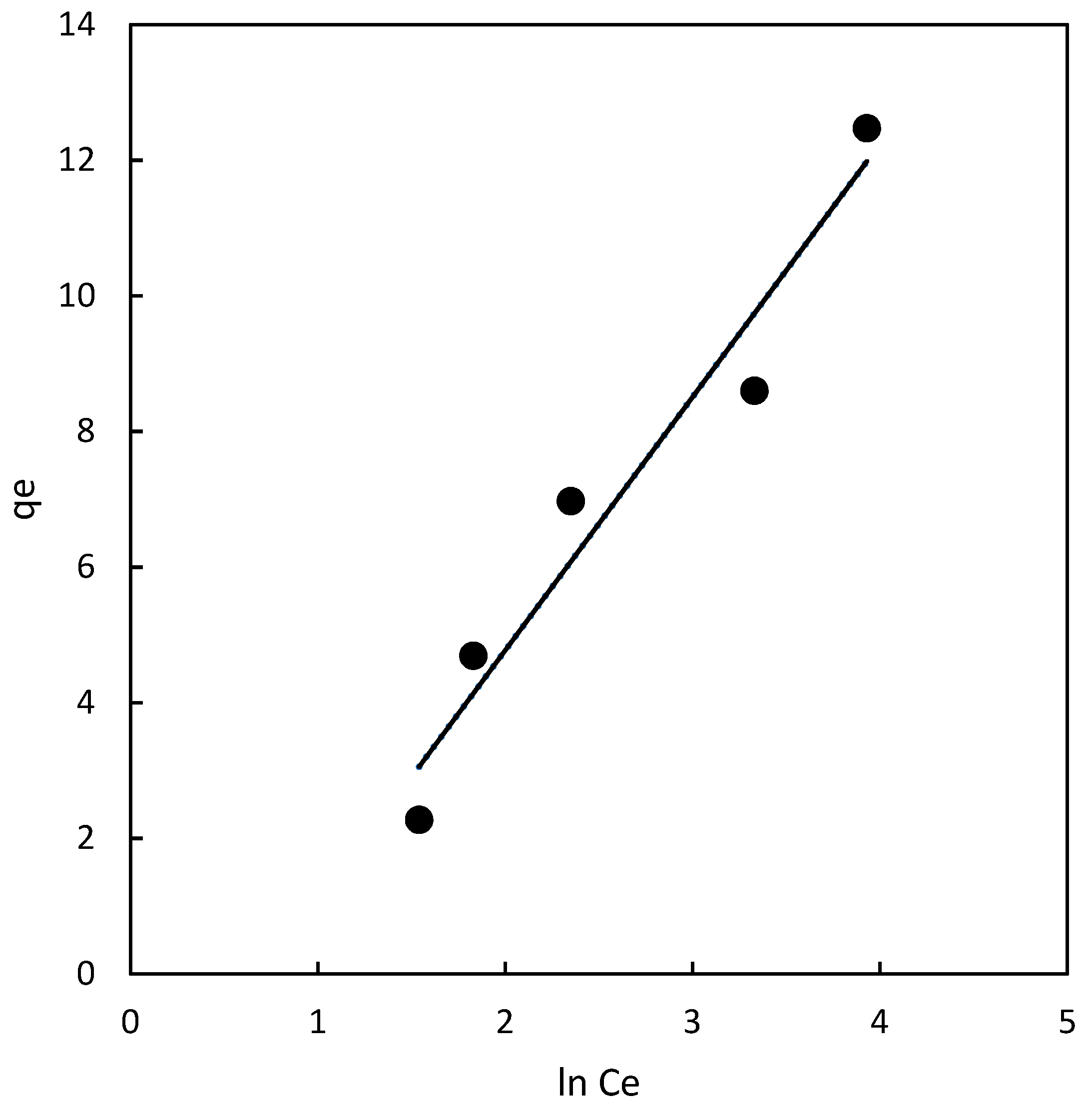
2.3.1. Freundlich Isotherm
The Freundlich isotherm is applicable to both monolayer (chemisorption) and multilayer adsorption (physisorption) processes and is based on the assumption that the adsorbate adsorbs onto the heterogeneous surface of the adsorbent. The Freundlich isotherm [25] provides two important constants, KF and nF, which reflect the adsorption capacity and intensity, respectively. For a favorable adsorption, the Freundlich constant nF typically falls within the range of 1 to 10. A higher value of nF (equivalently, a smaller value of 1/nF) indicates a stronger and more effective interaction between the adsorbent and the adsorbate. When 1/nF is less than 1, it corresponds to a normal L-type isotherm, while 1/nF greater than 1 indicates cooperative sorption.
According to the results presented in Table 2 and Figure 5, the KF value for the magnetic chitosan polymer was found to be 1.28. The most crucial parameter related to this isotherm is nF, which represents the heterogeneity factor. In the case of the chitosan magnetic polymer, the value of nF was determined to be 1.68, falling within the favorable adsorption range of 1 to 10. This suggests that the adsorption process is favored and that there is an effective interaction between the adsorbent and the adsorbate. The experimental data were fitted to the Freundlich model, resulting in a determination coefficient of 0.844 for the chitosan polymer. This coefficient represents the goodness of fit of the experimental data to the Freundlich isotherm model for the adsorption process.
2.3.2. Langmuir Isotherm
The Langmuir adsorption isotherm is based on the assumption of homogeneous adsorption, where adsorption occurs in a monolayer coverage on the adsorbent surface. This isotherm assumes that all adsorption sites are equivalent, leading to uniform surface coverage. According to the Langmuir model, the ability of a molecule to adsorb at a specific site is independent of the occupation of neighboring sites.
For the Langmuir isotherm, it is essential to analyze the qmax value, which represents the maximum adsorption capacity of the adsorbent under specific experimental conditions. In the case of the magnetic chitosan polymer, the qmax value was found to be 17.46 (Table 2, Figure 6A). This value provides valuable information about the adsorption capacity of the adsorbent and the maximum amount of dye that can be adsorbed per unit weight of the adsorbent.
2.3.3. Temkin Isotherm
The experimental data were also analyzed using the Temkin isotherm. The best fit for the magnetic chitosan polymer was achieved using this model with a determination coefficient of 0.946, indicating that the adsorption occurred on heterogeneous surfaces [24]. The Temkin isotherm model assumes that heat of adsorption (function of temperature) of all molecules in the layer would decrease linearly rather than logarithmic with coverage. The Temkin isotherm model mainly describes the chemical adsorption process as electrostatic interaction. In the present study, the Temkin isotherm fitted the observed results well, hence, electrostatic interaction is an important mechanism affecting the interaction be-tween the chitosan adsorbent and the pollutant [25].
Figure 7.
Temkin isotherm plot for chitosan magnetic polymer.
2.3. Polymer Characterization
2.3.1. Thermogravimetric Analysis
Different pattern of decomposition was obtained for the original chitosan and the iron oxide coated polymer (Figure 8).
Together with a first mass loss, probably due to water hydration (below 150° C) a single decomposition path was observed for chitosan. Common elimination of volatile compounds at similar temperatures was also recorded for the iron polymer, followed by another four not completely defined steps leading to a total mass loss of 36.05%. No defined major compounds or stable intermediates were identified within the MS fragments, with multiple masses between 30 and 73 amu, probably corresponding to the decomposition series of oxygen and nitrogen single bonded compounds Cn H2n+1 O and Cn H2n+2 N.
The major weight loss in chitosan above 300 degrees, where most of the organic matter is lost, was not observed in the iron containing polymer. However, the second and third losses, occurring between 150 and 400 degrees are very similar to those suffered by the iron particles although to a higher extent (8.42 and 4.09% in the polymer towards 1.56 and 0.85% in the iron particles).
A last significant loss of 7.65% by weight above 700 degrees was registered leaving a total mass loss almost halved (from 67.91% to 36.05%) than original chitosan with about 64% of matter remaining after the constant heating up to 800 °C (Figure 8B).
From thermogravimetry, the weight percentage of chitosan in the Chitosan-Fe polymer can be calculated as follows [26]:
where the Ws was the weight loss (%) from 120 to 800 °C for the chitosan-Fe samples, and Wn was the weight loss (%) from 120 to 800 °C for the pure Fe3O4 nanoparticles. After calculation, the weight percentage of chitosan in chitosan-Fe reached 31.5 %. In the case of Jaafari’s chitosan-Fe nanoparticles [24] they obtain 16.3%. The double content in organic matter obtained for the in situ generation of iron particles could suggest a higher efficiency in the incorporation into the structure of the polymer.
Chitosan
content = Ws (%) - Wn (%)
2.3.2. DRX Powder X-ray Diffraction
A degree of crystallinity between 68-70% was recorded in the material for the independently prepared iron particles (PI) and for the chitosan polymer formed in the presence of iron particles (CHI-Fe). The characteristic face-centred cubic lattice Fd-3m of magnetite (ICDD database, standard sample PDF 04-006-6551) observed for independently PI particles diffraction pattern is majorly found in the final chitosan iron polymer (Figure 9).
However, novel diffractions were also observed together with those of magnetite which could be attributed to a distortion of the crystalline structure or to a substitution of magnetite by haematite in some lattices. This last process has been previously described by a partial oxidative substitution of Fe2+ or through a redox-independent dissolution-reprecipitation reaction in the acidic media in which they are prepared [27].
2.3.3. IRTF
Similar profiles were observed in the spectrum of commercial chitosan and iron containing chitosan polymer (Figure 10).
The absorption bands at 2916 and 2868 cm−1 attributed to C-H symmetric and asymmetric stretching, respectively, were also recorded for the polymer with a lower definition. The stretching vibration of the double bound C=O (1654 cm-1) with minor intensity than the N–H (3355.42 cm-1), typical for chitosan and related polysaccharides, was also found for both compounds although at slightly higher frequencies in the case of the polymer.
This shift of the bands to lower frequencies (C=O bands 1654.16 and 1678.75 and NH at 1589 to 1560 cm-1 can be attributed to the establishment of new hydrogen bridge interactions that weaken the bonds vibrating in the structure. On the other hand, both the C-N stretching vibration bands, originally located at 1419.85 cm-1, 1378.63 and 1319.67 cm-1 and the C-O bands at 1062.12, 1022.52 and 984.01 cm-1 are shifted to higher frequencies 1459.14, 1407, and 1057.84, 1018.19, which is an evidence of an increasement in the strain of the structure when forming the coating for the iron particles.
Finally, a significant band corresponding to the vibration of the iron-oxygen bonds at 534 cm-1 was also identified in the spectrum.
2.3.4. SEM and EDX
Several representative polymeric macrostructures were analyzed by field emission scanning electron microscopy to characterize the morphology of iron coated chitosan polymer. Highly regular spherical structures were observed for the polymer (Figure 11A). However, some small dark areas dotted the structure suggesting the presence of zones where the coating of iron nanoparticles seems to be not completed (Figure 11B).
The EDX analysis revealed a huge difference in iron content for both structures (Figure 12), being virtually absent in clear areas and the majority in dark ones, and thus supporting the previous assumption.
2.3.5. Molecular Models
The interaction of chitosan with iron was eventually assessed by using density functional theory (DFT). Simulations were performed with divalent cations and glucosamine monomers, a model system by Gomes and co-workers that correctly mimics the stability of chitosan complexes with metallic ions [28]. As discussed by these authors, metal centres can be coordinate to chitosan by hydroxyl and/or amino groups at five available sites (labelled as C1 – C5). Figure 13 illustrates the optimized complexes with metals at these positions. Values in parenthesis stand for the computed relative energies in kcal/mol, where the global minimum is taken as reference. As noted, the C3 coordination leads to the most stable complex, while all other coordination patterns are associated to less favourable (more positive) relative energies, which lie in the range of 13.14 – 29.21 kcal/mol. Indeed, C3 outperforms both the anchoring to the amino groups of the chitosan entity (C4 and C5) and the alternative C1 and C2 sites, even if the former established three interactions (two hydroxyl contacts + the heterocyclic oxygen). A close inspection of Figure 13 reveals that the large stability at C3 arises from a concomitant proton transfer equilibrium from the hydroxyl to the amino group. Consequently, theory predicts that iron coordination induces a protonation transfer that leads to a deprotonated hydroxyl, which in turn enhances the coordination. This computational outcome agrees the recorded IR spectrum, where Fe – O bands are observed while Fe – N peaks were not present.
3. Materials and Methods
3.1. Chemicals and Reagents
Chitosan, iron (III) chloride hexahydrate (FeCl3·6H2O), ammonium hydroxide, and ethanol were procured from Sigma-Aldrich (Spain). Meanwhile, iron (II) chloride tetrahydrate (FeCl2·4H2O) was obtained from Fluka (Spain). The Direct Red 83:1 dye used in the experiments was supplied by AITEX (Asociación de Investigación de la Industria Textil, Alcoy, Spain).
3.2. Iron Nanoparticles Preparation
In order to compare possible differences in the structure and efficacy of the incorporation into the polymer between iron oxide nanoparticles performed by classical co-precipitation under alkaline conditions and in situ formation in acidic media during polymerization of chitosan, magnetic nanoparticles were also prepared following a standard procedure as follows. 3.49 g of FeCl2·4H2O and 9.5 g of FeCl3·6H2O were sequentially dissolved in 100 mL of water at room temperature. After complete solution, 30 mL of ammonium hydroxide was added drop by drop and the mixture was subjected to magnetic stirring for 30 minutes at 80 °C to promote proper reaction and particle formation. The mixture was then centrifuged at 4000 rpm for 10 minutes to separate the solid precipitate from the liquid solution. The resulting precipitate was then washed twice with a mixture of ethanol and water in a 1:1 ratio to remove basic medium and unreacted reagents. Finally, the washed precipitate was left to dry overnight, resulting in the formation of magnetic nanoparticles. These magnetic nanoparticles are now ready for use in further experiments or applications.
3.3. Chitosan-Fe Polymer Preparation
To prepare the chitosan magnetic beads, the following procedure was followed. 5 g of chitosan powder was dissolved in 250 mL of a 5% acetic acid aqueous solution. The mixture was stirred for 2 hours at 50 °C to obtain a homogeneous gel. After achieving a uniform gel, 16 g of FeCl2·4H2O and 32 g of FeCl3·6H2O were added to the gel. The mixture was further stirred for 1 hour at 50 °C to facilitate the incorporation of iron ions into the gel. To form the polymer beads, the homogeneous gel containing chitosan and iron ions was carefully dropped into a bath containing a 30% aqueous solution of NaOH. Upon contact with the NaOH solution, the gel rapidly transformed into spherical particles, thus forming the chitosan magnetic beads. The newly formed beads were then washed with water to remove any residual chemicals or impurities. Finally, the chitosan magnetic beads were left to dry at room temperature, resulting in the final product, ready for use in the experiments.
3.4. Dye solution Preparation
To conduct the adsorption experiments, various concentrations of Direct Red 83:1 were prepared. Direct Red 83:1 is an azo dye with the chemical formula C33H20N6Na4O17S4 and a molecular weight of 992.77 g/mol.
The concentrations of Direct Red 83:1 used in the adsorption tests for both adsorbents were as follows: 50 mg/L, 100 mg/L, 150 mg/L, 200 mg/L, and 300 mg/L. These different concentrations were employed to investigate and evaluate the adsorption properties of the respective adsorbents under varying dye concentrations. By analyzing the adsorption behavior at different dye concentrations, a comprehensive understanding of the adsorption process and efficiency can be obtained.
3.5. Analyses and Data Evaluation
In the adsorption experiments, the concentration of the dye in the supernatant was measured using a spectrophotometer, specifically the Shimadzu UV-1700 model (Kyoto, Japan). The measurements were taken after reaching the equilibrium state between the dye and the adsorbents. The absorbance of the dye solution was measured both before and after the treatment with the polymers at the wavelength of maximum absorbance for the dye, which is λmax = 526 nm. The molar absorptivity (extinction coefficient) of the dye at this wavelength is ε526 = 1065 M-1cm-1.
By comparing the absorbance values before and after the treatment, the extent of dye adsorption onto the polymers can be determined. This analysis helps in evaluating the effectiveness of the adsorbents in removing the dye from the solution at different concentrations.
3.6. Adsorption Experiments
The adsorption tests were conducted at a constant temperature of 25 °C, utilizing solutions containing various concentrations of the dye ranging from 50 to 300 mg/L. For each experiment, 1g of the polymer was mixed with 50 mL of the dye solution. The mixture was continuously stirred at a fixed speed of 500 rpm throughout the experiment to ensure uniform contact between the dye and the adsorbent.
To determine the amount of dye that was not retained by the polymer at specific time intervals (every 10 minutes), external magnets were employed. The mixture was subjected to the influence of these magnets for 5 minutes, facilitating the separation of the magnetic polymer beads along with the adsorbed dye from the solution.
Once the separation was accomplished, the concentration of the remaining dye in the solution was measured using the spectrophotometer, which allows for precise and accurate quantification of the dye’s concentration. This procedure was repeated for each concentration of dye tested, and the data obtained from the spectrophotometer measurements were used to assess the adsorption efficiency of the polymer under varying dye concentrations and contact times.
The amount of dye adsorbed on the polymers (qt) in mg/g was determined using a mass balance approach, as described by Renard et al. in 1997 [29]. The equation used for this determination is given by Equation (9):
where:
- qt is the amount of dye adsorbed on the polymer at time t (mg/g).
- Co is the initial concentration of dye in the solution (mg/L).
- Ct is the concentration of dye in the solution at time t (mg/L).
- V is the volume of the dye solution used (L).
- m is the mass of the polymer used (g)
3.7. Adsorption Kinetics
The study of kinetics holds significant importance in adsorption research as it allows us to predict the rate at which pollutants are eliminated from aqueous solutions and provides valuable insights into the mechanism of sorption reactions. To gain a deeper understanding of the mechanism behind dye adsorption onto the newly developed adsorbents, several kinetic models, including the pseudo first order, pseudo second order, and intra-particle diffusion models, were carefully examined using the experimental data. These models were utilized to analyze and characterize the adsorption process, enabling a comprehensive investigation of the interactions between the adsorbents and the dye molecules.
3.8. Isotherm Analysis
The adsorption isotherm plays a critical role in understanding how adsorbing molecules are distributed between the liquid and solid phases once the adsorption process reaches an equilibrium state. To optimize the design of an adsorption system for efficiently removing Direct Red 83:1 from solutions, it becomes crucial to identify the most suitable correlation for the equilibrium studies. In this study, three different isotherms, namely Freundlich, Langmuir, and Temkin isotherms, were employed and fitted to the experimental data.
By utilizing these isotherms, the adsorption behavior of Direct Red 83:1 onto the adsorbents can be thoroughly investigated, and the appropriate model can be selected based on its best fit to the experimental data. This choice will aid in obtaining valuable information about the adsorption capacity, surface characteristics, and interactions between the adsorbent and the dye molecules, ultimately contributing to the optimal design and performance of the adsorption system.
3.9. Polymer Characterization
Thermogravimetric analysis was performed on a thermobalance model TGA/DSC 1 HT (Mettler-Toledo GmbH, Schwerzenbach, Switzerland) coupled to a Balzers Thermostar mass spectrometer (Pfeiffer Vacuum, Asslar, Germany) for gas analysis. Scan bargraph cycles were performed in the range 15–94 m/z in the quadrupole mass spectrometer (QMS 200 M3), with a dwell time of 2 s for every ion and cathode voltage in the ion source of 65 V.
About 10 mg of sample were used to study the thermal decomposition from 30 to 800 °C at a heating rate of 10 °C/min under N2 atmosphere with a flow rate of 50 mL/min. During the experiment, the sample was placed in an uncovered sapphire crucible of 70 μL capacity. The result was corrected with a blank curve. For each sample, the m/z-ratio profiles in the range 15-94 amu, the experimental mass loss (TG curve) and its first derivative (DTG curve) were recorded.
The crystalline phases in pre-formed iron nanoparticles and within the polymer were also analysed. An x-ray powder diffractometer in mode θ-θ (Bruker D8 Advance, Bruker Corporation, Billerica, MA, USA), using Cu Kα radiation at 40 kV and 30 mA and one dimensional detector with a 2° window. The primary optics consisted of a 2° Soller slit, a 1 mm incidence slit and an air anti-scattering screen. The secondary optics included an 8 mm anti-scattering slit, a Ni filter and a 2.5° Soller slit.
Approximately 1 g of powder reduced iron coated macrostructures was placed on a back-loaded sample holder and analysed at steps of 0.05º (dwell time of 1 s/step) over an angular range of 10-70° and 30 rpm of angular velocity. The powder diffraction file was evaluated with the linked software (DIFFRAC.EVA 5.2, Bruker AXS, 2020, MA, USA) and a crystalline powder database (PDF-4+ 2021, ICDD).
The infrared study was performed on a Nicolet 5700 spectrometer (Nicolet, Madison, WI, USA) equipped with a Ge/KBr beam splitter, a DTGS-KBr detector and a ceramic infrared source. The sampling module was the Smart Orbit diamond attenuated total reflectance attenuator accessory. The samples were analyzed finely divided and pre-dried at 60 °C. Spectral analysis was performed in the range 4000 to 400 cm-1, with a resolution of 4 cm-1.
FESEM uncovered samples mounted with the aid of conductive carbon cement on aluminum stubs. FESEM-EDX analyses were performed with a FE-SEM (ApreoS Lovac IML Thermofisher, MA, USA) and coupled with an Octane Plus EDAX microanalyzer (AMETEK, PA, USA). Sample analysis were performed between 1 - 2 kV, and 20 kV for EDX analysis.
3.10. Computational Calculations
All DFT calculations were performed with the Gaussian 16 suite of programs [30]. The molecular structures were fully optimized with the dispersion-corrected version of the B3LYP functional (B3LYP-D3) [31,32]. This functional has been successfully used for simulating chitosan-metal complexes [33]. The Def2SVP basis set was used for all atoms except Fe, which was treated with the relative effective core potentials (Def2-ECP) [34,35]. Frequencies were also computed to confirm that the localized structures correctly correspond to real minima in the potential energy surface.
4. Conclusions
Chitosan-Fe polymer can be successfully used in removing of Direct red 83:1. The process of adsorption in polymer was found to be better described by the pseudo-second-order kinetic model with a good determination coefficient (R2=0.999). The adsorption equilibrium of Direct Red 83:1 was suitably described by the Temkin isotherm, being the maximum adsorption capacity of 17.46 mg/g (qmax). Its magnetic properties make it easily separable from water to accomplish a refined cleaning. The determinations carried out by thermogravimetry, differential scanning calorimetry, and Fourier transform infrared spectrometry on isolated reactants and their respective complexes confirm that, in all cases, complex formation between the Direct Red 83:1 under study and Chitosan-Fe polymer is effective. The complexation of Chitosan-Fe with the dye seems suitable to reduce the environmental impact of the dyeing industry.
Author Contributions
The authors who sign the following manuscript have made significant contributions, allowing achieving the set objectives: E.N.-D. and J.A.G. were responsible for the conception, design and assessment of the work. Also, revised and corrected the manuscript previous remission; Iron nanoparticles preparation; chitosan-iron polymer preparation; the adsorption experiments and interpretation of the results were carried out by A.M-S., M.I.R.-L. and T.G-M.; J.A.P accomplish the adsorption kinetics and interpretation of adsorption isotherm models to know the interaction of the dye with the polymer adsorbent, also contributing in the manuscript writing; M.J.Y-G. and D.A. carried out the characterization of the polymer through elemental analysis of the composition, the polymer micrographies by FESEM, given as consequence a plausible explanation of their morphology; D.A and J.P.C-C. accomplish the IR spectra, thermogravimetric analysis, and also carried out and interpreted the computational studies.
Funding
This research was supported by the European project “CLEANUP” (Validation of adsorbent materials and advanced oxidation techniques to remove emerging pollutants in treated wastewater, LIFE 16 ENV/ES/000169).
Conflicts of Interest
The authors declare no conflict of interest.
References
- Ahmed, J.; Thakur, A.; Goyal, A. Industrial Wastewater and Its Toxic Effects. In Biological Treatment of Industrial Wastewater; Shah, M. P., Ed.; The Royal Society of Chemistry, 2021; pp. 1–14. [CrossRef]
- Markandeya; Mohan, D.; Shukla, S.P. Hazardous Consequences of Textile Mill Effluents on Soil and Their Remediation Approaches. Cleaner Engineering and Technology 2022, 7, 100434. [Google Scholar] [CrossRef]
- Azanaw, A.; Birlie, B.; Teshome, B.; Jemberie, M. Textile Effluent Treatment Methods and Eco-Friendly Resolution of Textile Wastewater. Case Studies in Chemical and Environmental Engineering 2022, 6, 100230. [Google Scholar] [CrossRef]
- Rápó, E.; Tonk, S. Factors Affecting Synthetic Dye Adsorption; Desorption Studies: A Review of Results from the Last Five Years (2017–2021). Molecules 2021, 26, 5419. [Google Scholar] [CrossRef] [PubMed]
- Rodríguez-López, M.I.; Pellicer, J.A.; Gómez-Morte, T.; Auñón, D.; Gómez-López, V.M.; Yáñez-Gascón, M.J.; Gil-Izquierdo, Á.; Cerón-Carrasco, J.P.; Crini, G.; Núñez-Delicado, E.; Gabaldón, J.A. Removal of an Azo Dye from Wastewater through the Use of Two Technologies: Magnetic Cyclodextrin Polymers and Pulsed Light. IJMS 2022, 23, 8406. [Google Scholar] [CrossRef] [PubMed]
- Al-Sakkaf, B.M.; Nasreen, S.; Ejaz, N. Degradation Pattern of Textile Effluent by Using Bio and Sono Chemical Reactor. Journal of Chemistry 2020, 2020, 1–13. [Google Scholar] [CrossRef]
- Morin-Crini, N.; Lichtfouse, E.; Fourmentin, M.; Ribeiro, A.R.L.; Noutsopoulos, C.; Mapelli, F.; Fenyvesi, É.; Vieira, M.G.A.; Picos-Corrales, L.A.; Moreno-Piraján, J.C.; Giraldo, L.; Sohajda, T.; Huq, M.M.; Soltan, J.; Torri, G.; Magureanu, M.; Bradu, C.; Crini, G. Removal of Emerging Contaminants from Wastewater Using Advanced Treatments. A Review. Environ Chem Lett 2022, 20, 1333–1375. [Google Scholar] [CrossRef]
- Keshvardoostchokami, M.; Majidi, M.; Zamani, A.; Liu, B. A Review on the Use of Chitosan and Chitosan Derivatives as the Bio-Adsorbents for the Water Treatment: Removal of Nitrogen-Containing Pollutants. Carbohydrate Polymers 2021, 273, 118625. [Google Scholar] [CrossRef] [PubMed]
- Kyzas, G.Z.; Bikiaris, D.N.; Mitropoulos, A.C. Chitosan Adsorbents for Dye Removal: A Review: Chitosan Adsorbents for Dye Removal. Polym. Int. 2017, 66, 1800–1811. [Google Scholar] [CrossRef]
- Da Silva Alves, D.C.; Healy, B.; Pinto, L.A.D.A.; Cadaval, T.R.S.; Breslin, C.B. Recent Developments in Chitosan-Based Adsorbents for the Removal of Pollutants from Aqueous Environments. Molecules 2021, 26, 594. [Google Scholar] [CrossRef]
- Nithya, R.; Thirunavukkarasu, A.; Sathya, A.B.; Sivashankar, R. Magnetic Materials and Magnetic Separation of Dyes from Aqueous Solutions: A Review. Environ Chem Lett 2021, 19, 1275–1294. [Google Scholar] [CrossRef]
- Pellicer, J.; Rodríguez-López, M.; Fortea, M.; Lucas-Abellán, C.; Mercader-Ros, M.; López-Miranda, S.; Gómez-López, V.; Semeraro, P.; Cosma, P.; Fini, P.; Franco, E.; Ferrándiz, M.; Pérez, E.; Ferrándiz, M.; Núñez-Delicado, E.; Gabaldón, J. Adsorption Properties of β- and Hydroxypropyl-β-Cyclodextrins Cross-Linked with Epichlorohydrin in Aqueous Solution. A Sustainable Recycling Strategy in Textile Dyeing Process. Polymers 2019, 11, 252. [Google Scholar] [CrossRef] [PubMed]
- Lagergren, S. Zur Theorie Der Sogenannten Adsorption Geloster Stoffe. Kungliga svenska vetenskapsakademiens. Handlingar 1898, 24, 1–39. [Google Scholar]
- Ho, Y.-S. Review of Second-Order Models for Adsorption Systems. ChemInform 2006, 37. [Google Scholar] [CrossRef]
- Weber, W.J., Jr.; Morris, J.C. Kinetics of Adsorption on Carbon from Solution. Journal of the sanitary engineering division 1963, 89, 31–59. [Google Scholar] [CrossRef]
- Wang, D.; Liu, L.; Jiang, X.; Yu, J.; Chen, X. Adsorption and Removal of Malachite Green from Aqueous Solution Using Magnetic β-Cyclodextrin-Graphene Oxide Nanocomposites as Adsorbents. Colloids and Surfaces A: Physicochemical and Engineering Aspects 2015, 466, 166–173. [Google Scholar] [CrossRef]
- Chen, B.; Chen, S.; Zhao, H.; Liu, Y.; Long, F.; Pan, X. A Versatile β-Cyclodextrin and Polyethyleneimine Bi-Functionalized Magnetic Nanoadsorbent for Simultaneous Capture of Methyl Orange and Pb(II) from Complex Wastewater. Chemosphere 2019, 216, 605–616. [Google Scholar] [CrossRef]
- Guo, Z.; Li, Y.; Pan, S.; Xu, J. Fabrication of Fe3O4@ Cyclodextrin Magnetic Composite for the High-Efficient Removal of Eu (III). Journal of Molecular Liquids 2015, 206, 272–277. [Google Scholar] [CrossRef]
- Liu, D.; Huang, Z.; Li, M.; Sun, P.; Yu, T.; Zhou, L. Novel Porous Magnetic Nanospheres Functionalized by β-Cyclodextrin Polymer and Its Application in Organic Pollutants from Aqueous Solution. Environmental Pollution 2019, 250, 639–649. [Google Scholar] [CrossRef]
- Crini, G.; Peindy, H.N.; Gimbert, F.; Robert, C. Removal of CI Basic Green 4 (Malachite Green) from Aqueous Solutions by Adsorption Using Cyclodextrin-Based Adsorbent: Kinetic and Equilibrium Studies. Separation and Purification Technology 2007, 53, 97–110. [Google Scholar] [CrossRef]
- Murcia-Salvador, A.; Pellicer, J.A.; Fortea, M.I.; Gómez-López, V.M.; Rodríguez-López, M.I.; Núñez-Delicado, E.; Gabaldón, J.A. Adsorption of Direct Blue 78 Using Chitosan and Cyclodextrins as Adsorbents. Polymers 2019, 11, 1003. [Google Scholar] [CrossRef] [PubMed]
- Pellicer, J.A.; Rodríguez-López, M.I.; Fortea, M.I.; Gabaldón Hernández, J.A.; Lucas-Abellán, C.; Mercader-Ros, M.T.; Serrano-Martínez, A.; Núñez-Delicado, E.; Cosma, P.; Fini, P.; Franco, E.; García, R.; Ferrándiz, M.; Pérez, E.; Ferrándiz, M. Removing of Direct Red 83:1 Using α- and HP-α-CDs Polymerized with Epichlorohydrin: Kinetic and Equilibrium Studies. Dyes and Pigments 2018, 149, 736–746. [Google Scholar] [CrossRef]
- Bensalah, H.; Younssi, S.A.; Ouammou, M.; Gurlo, A.; Bekheet, M.F. Azo Dye Adsorption on an Industrial Waste-Transformed Hydroxyapatite Adsorbent: Kinetics, Isotherms, Mechanism and Regeneration Studies. Journal of Environmental Chemical Engineering 2020, 8, 103807. [Google Scholar] [CrossRef]
- Jaafari, J.; Barzanouni, H.; Mazloomi, S.; Amir Abadi Farahani, N.; Sharafi, K.; Soleimani, P.; Haghighat, G.A. Effective Adsorptive Removal of Reactive Dyes by Magnetic Chitosan Nanoparticles: Kinetic, Isothermal Studies and Response Surface Methodology. International Journal of Biological Macromolecules 2020, 164, 344–355. [Google Scholar] [CrossRef] [PubMed]
- Hu, Q.; Lan, R.; He, L.; Liu, H.; Pei, X. A Critical Review of Adsorption Isotherm Models for Aqueous Contaminants: Curve Characteristics, Site Energy Distribution and Common Controversies. Journal of Environmental Management 2023, 329, 117104. [Google Scholar] [CrossRef]
- Zhang, L.; Zhu, X.; Sun, H.; Chi, G.; Xu, J.; Sun, Y. Control Synthesis of Magnetic Fe3O4–Chitosan Nanoparticles under UV Irradiation in Aqueous System. Current Applied Physics 2010, 10, 828–833. [Google Scholar] [CrossRef]
- Otake, T.; Wesolowski, D.J.; Anovitz, L.M.; Allard, L.F.; Ohmoto, H. Mechanisms of Iron Oxide Transformations in Hydrothermal Systems. Geochimica et Cosmochimica Acta 2010, 74, 6141–6156. [Google Scholar] [CrossRef]
- Gomes, J.R.B.; Jorge, M.; Gomes, P. Interaction of chitosan and chitin with Ni, Cu and Zn ions: A computational study. The Journal of Chemical Thermodynamics 2014, 73, 121–129. [Google Scholar] [CrossRef]
- Renard, P.; De Marsily, G. Calculating equivalent permeability: a review. Advances in water resources 1997, 20, 253–278. [Google Scholar] [CrossRef]
- Gaussian 16, Revision A.03, Frisch, M.J.; Trucks, G.W.; Schlegel, H.B.; Scuseria, G.E.; Robb, M.A.; Cheeseman, J.R.; Scalmani, G.; Barone, V.; Petersson, G.A.; Nakatsuji, H.; Li, X.; Caricato, M.; Marenich, A.V.; Bloino, J.; Janesko, B.G.; Gomperts, R.; Mennucci, B.; Hratchian, H.P.; Ortiz, J.V.; Izmaylov, A.F.; Sonnenberg, J.L.; Williams-Young, D.; Ding, F.; Lipparini, F.; Egidi, F.; Goings, J.; Peng, B.; Petrone, A.; Henderson, T.; Ranasinghe, D.; Zakrzewski, V.G.; Gao, J.; Rega, N.; Zheng, G.; Liang, W.; Hada, M.; Ehara, M.; Toyota, K.; Fukuda, R.; Hasegawa, J.; Ishida, M.; Nakajima, T.; Honda, Y.; Kitao, O.; Nakai, H.; Vreven, T.; Throssell, K.; Montgomery, J.A., Jr.; Peralta, J.E.; Ogliaro, F.; Bearpark, M.J.; Heyd, J.J.; Brothers, E.N.; Kudin, K.N.; Staroverov, V.N.; Keith, T.A.; Kobayashi, R.; Normand, J.; Raghavachari, K.; Rendell, A.P.; Burant, J.C.; Iyengar, S.S.; Tomasi, J.; Cossi, M.; Millam, J.M.; Klene, M.; Adamo, C.; Cammi, R.; Ochterski, J.W.; Martin, R.L.; Morokuma, K.; Farkas, O.; Foresman, J.B.; Fox, D.J.Gaussian, Inc., Wallingford CT, 2016.
- Grimme, S. Density functional theory with London dispersion corrections. Comput. Mol. Sci 2011, 1, 211–228. [Google Scholar] [CrossRef]
- Becke, A.D. A new mixing of Hartree−Fock and local density− functional theories. J. Chem. Phys. 1993, 98, 1372–1377. [Google Scholar] [CrossRef]
- Ataei, S.; Nemati-Kande; E. Bahrami, A. Quantum DFT studies on the drug delivery of favipiravir using pristine and functionalized chitosan nanoparticles. Sci Rep 2023, 13, 21984. [Google Scholar] [CrossRef] [PubMed]
- Weigend, F.; Ahlrichs, R. Balanced basis sets of split valence, triple zeta valence and quadruple zeta valence quality for h to rn: design and assessment of accuracy. Phys. Chem. Chem. Phys 2005, 7, 3297–3305. [Google Scholar] [CrossRef]
- Weigend, F. Accurate coulomb−fitting basis sets for H to Rn. Phys. Chem. Chem. Phys 2006, 8, 1057–1065. [Google Scholar] [CrossRef] [PubMed]
Figure 1.
Influence of contact time on chitosan adsorption capacity at various dye concentrations: 50 mg/L (•), 100 mg/L (■), 150 mg/L (♦), 200 mg/L (▲), and 300 mg/L (○).
Figure 1.
Influence of contact time on chitosan adsorption capacity at various dye concentrations: 50 mg/L (•), 100 mg/L (■), 150 mg/L (♦), 200 mg/L (▲), and 300 mg/L (○).
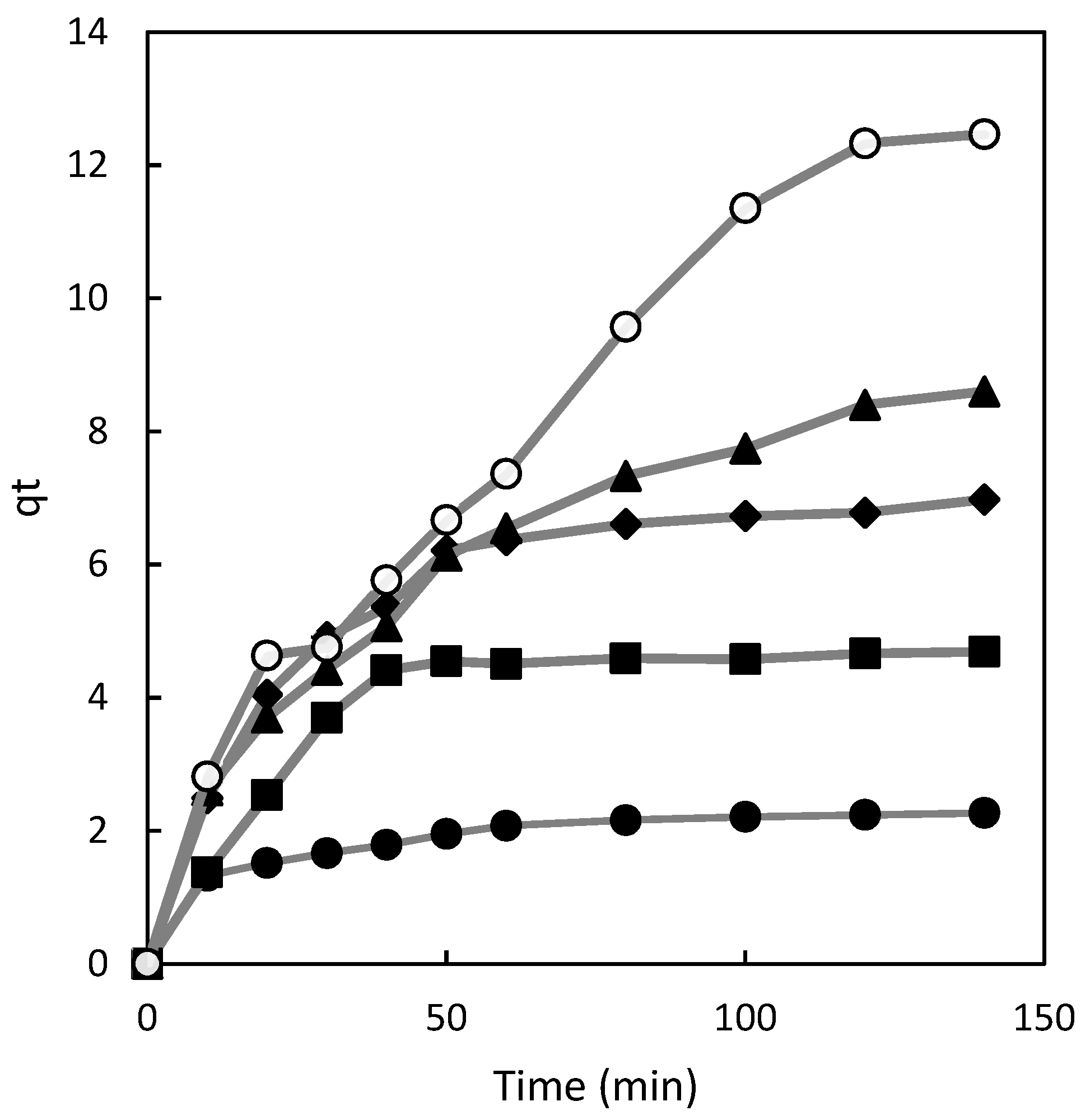
Figure 2.
Pseudo first order model plots for chitosan at different dye concentrations 50 mg/L (•), 100 mg/L (■), 150 mg/L (♦), 200 mg/L (▲) and 300 mg/L (○).
Figure 2.
Pseudo first order model plots for chitosan at different dye concentrations 50 mg/L (•), 100 mg/L (■), 150 mg/L (♦), 200 mg/L (▲) and 300 mg/L (○).
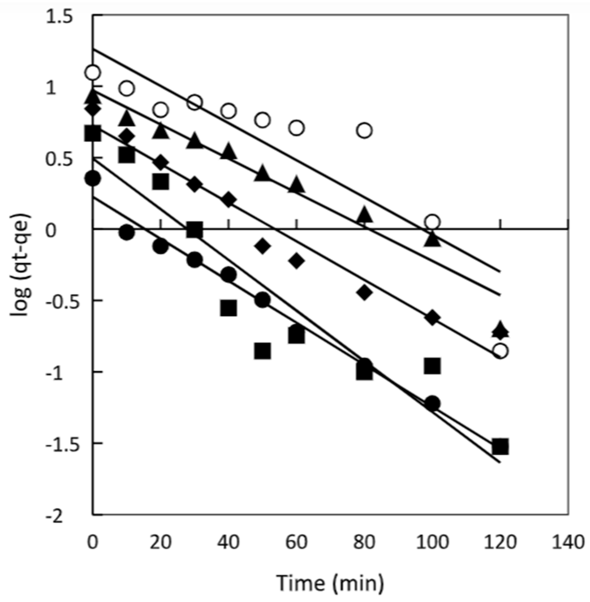
Figure 3.
Pseudo second order model plots for chitosan at different dye concentrations 50 mg/L (•), 100 mg/L (■), 150 mg/L (♦), 200 mg/L (▲) and 300 mg/L (○).
Figure 3.
Pseudo second order model plots for chitosan at different dye concentrations 50 mg/L (•), 100 mg/L (■), 150 mg/L (♦), 200 mg/L (▲) and 300 mg/L (○).
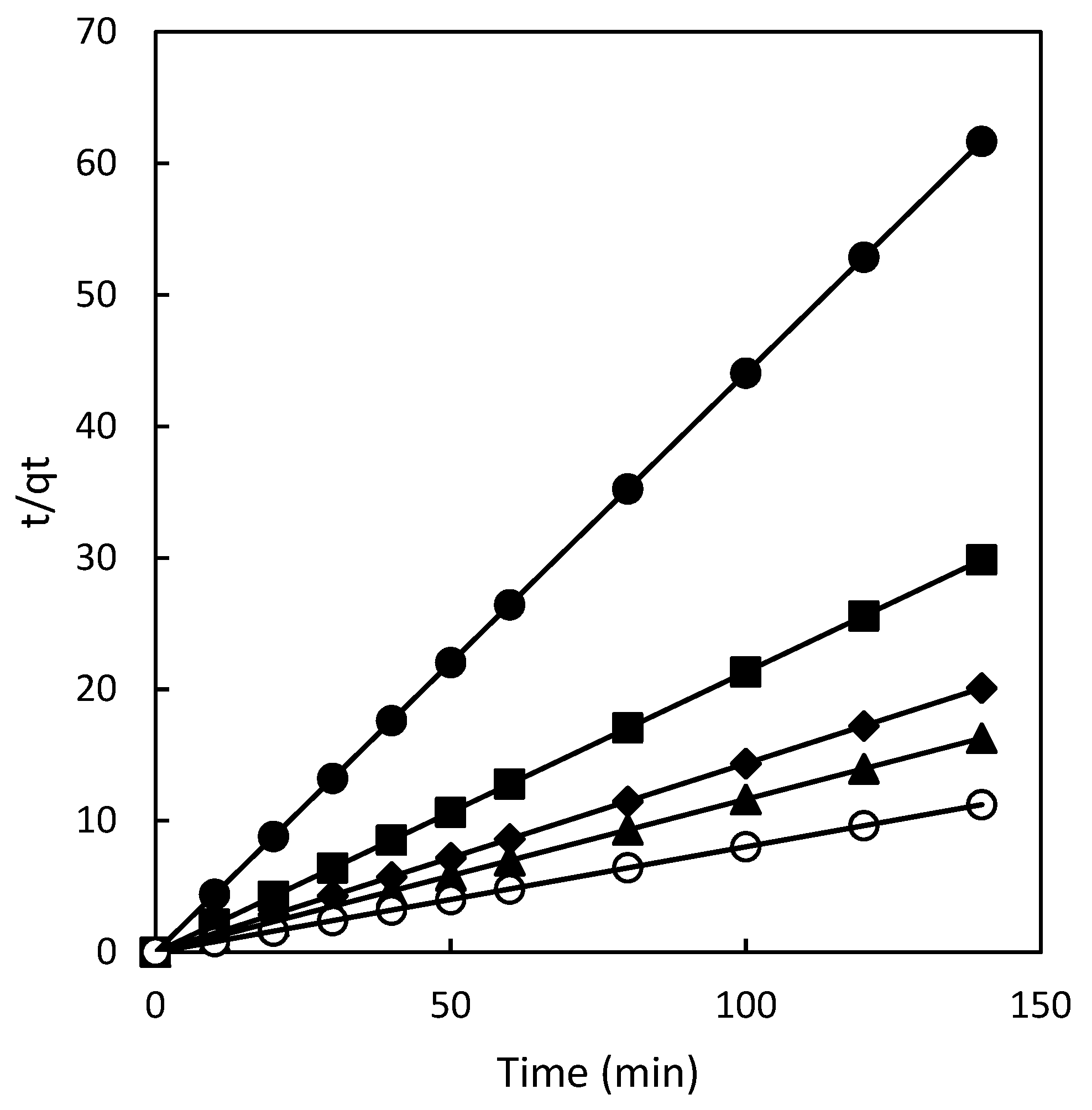
Figure 4.
Intraparticle diffusion model plots for chitosan at different dye concentrations 50 mg/L (•), 100 mg/L (■), 150 mg/L (♦), 200 mg/L (▲) and 300 mg/L (○).
Figure 4.
Intraparticle diffusion model plots for chitosan at different dye concentrations 50 mg/L (•), 100 mg/L (■), 150 mg/L (♦), 200 mg/L (▲) and 300 mg/L (○).
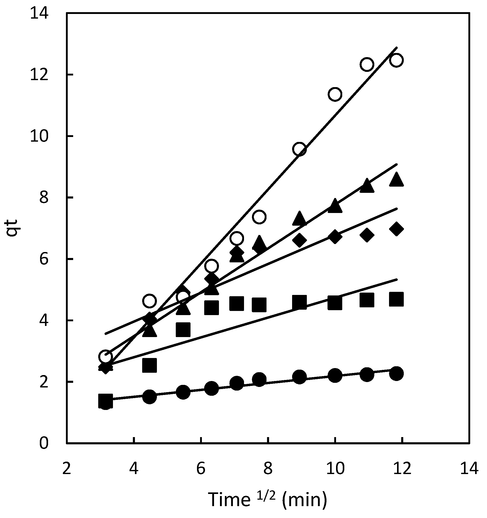
Figure 5.
Freundlich isotherm plot for chitosan magnetic adsorbent.
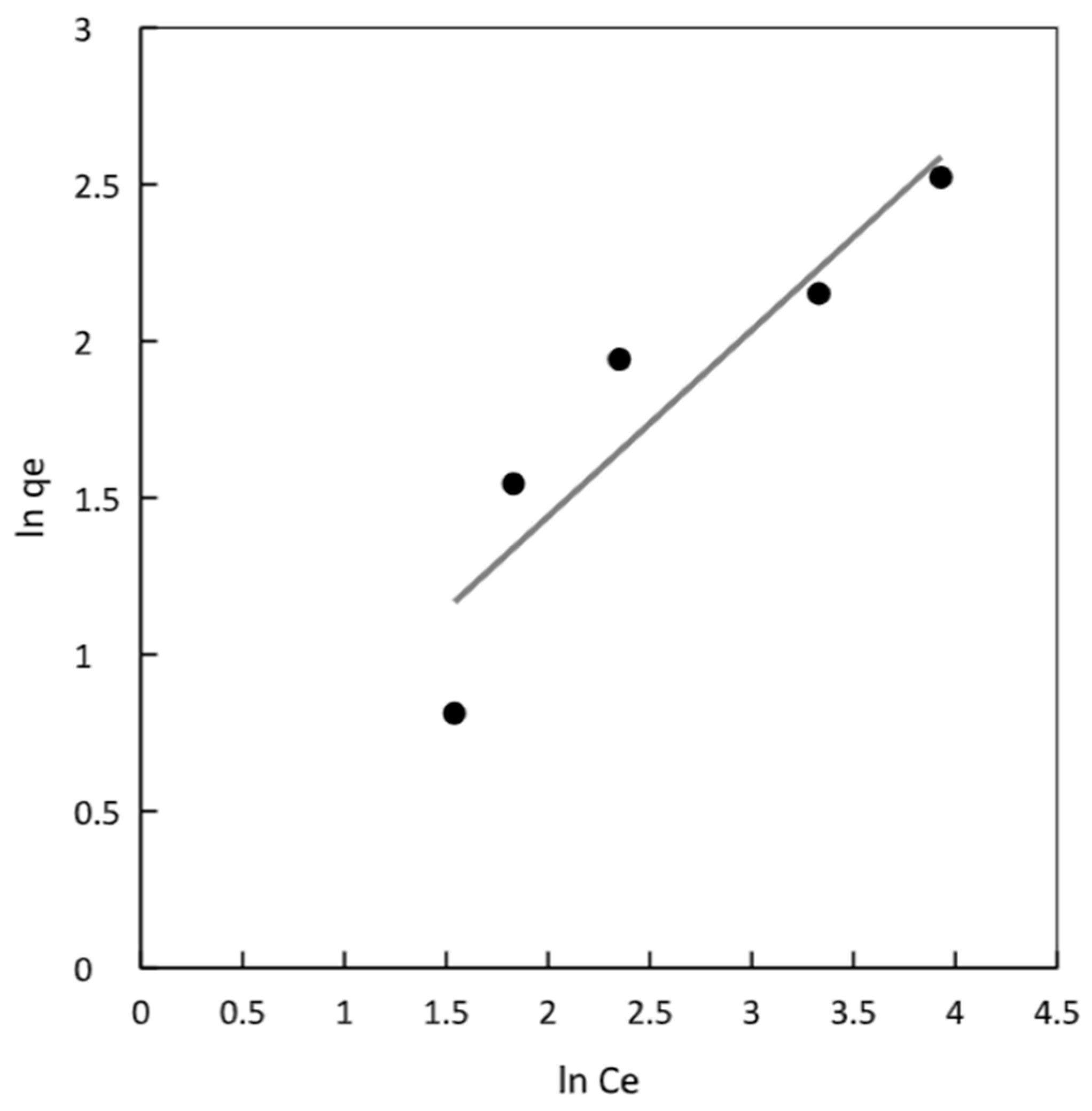
Figure 6.
(A). Langmuir isotherm plot. (B) Separation factor.
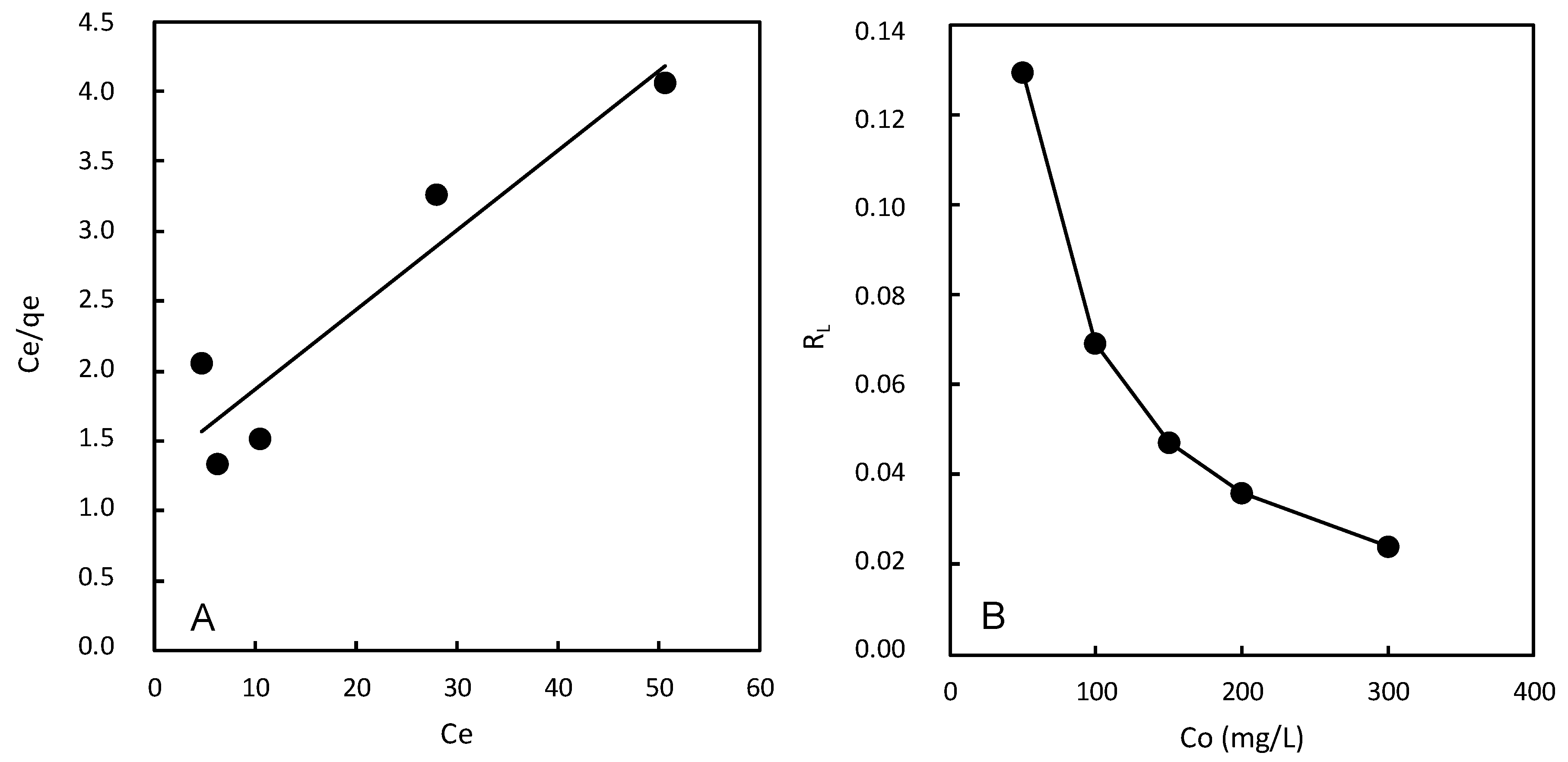
Figure 8.
A TG of chitosan-Fe (Blue line), chitosan (Grey Line) and Fe (Orange line). B. DTG of chitosan-Fe (Blue line), chitosan (Grey Line) and Fe (Orange line).
Figure 8.
A TG of chitosan-Fe (Blue line), chitosan (Grey Line) and Fe (Orange line). B. DTG of chitosan-Fe (Blue line), chitosan (Grey Line) and Fe (Orange line).
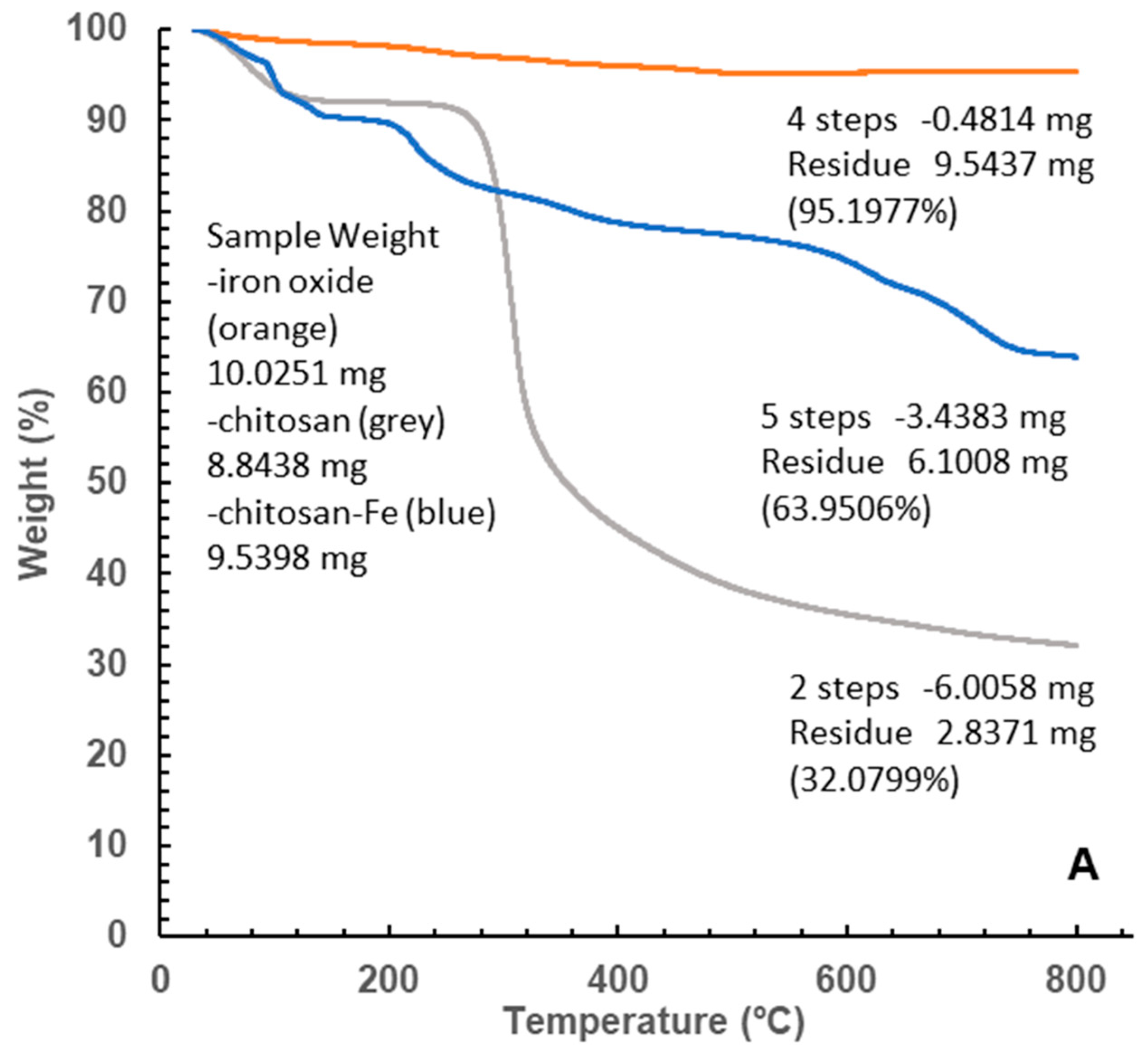
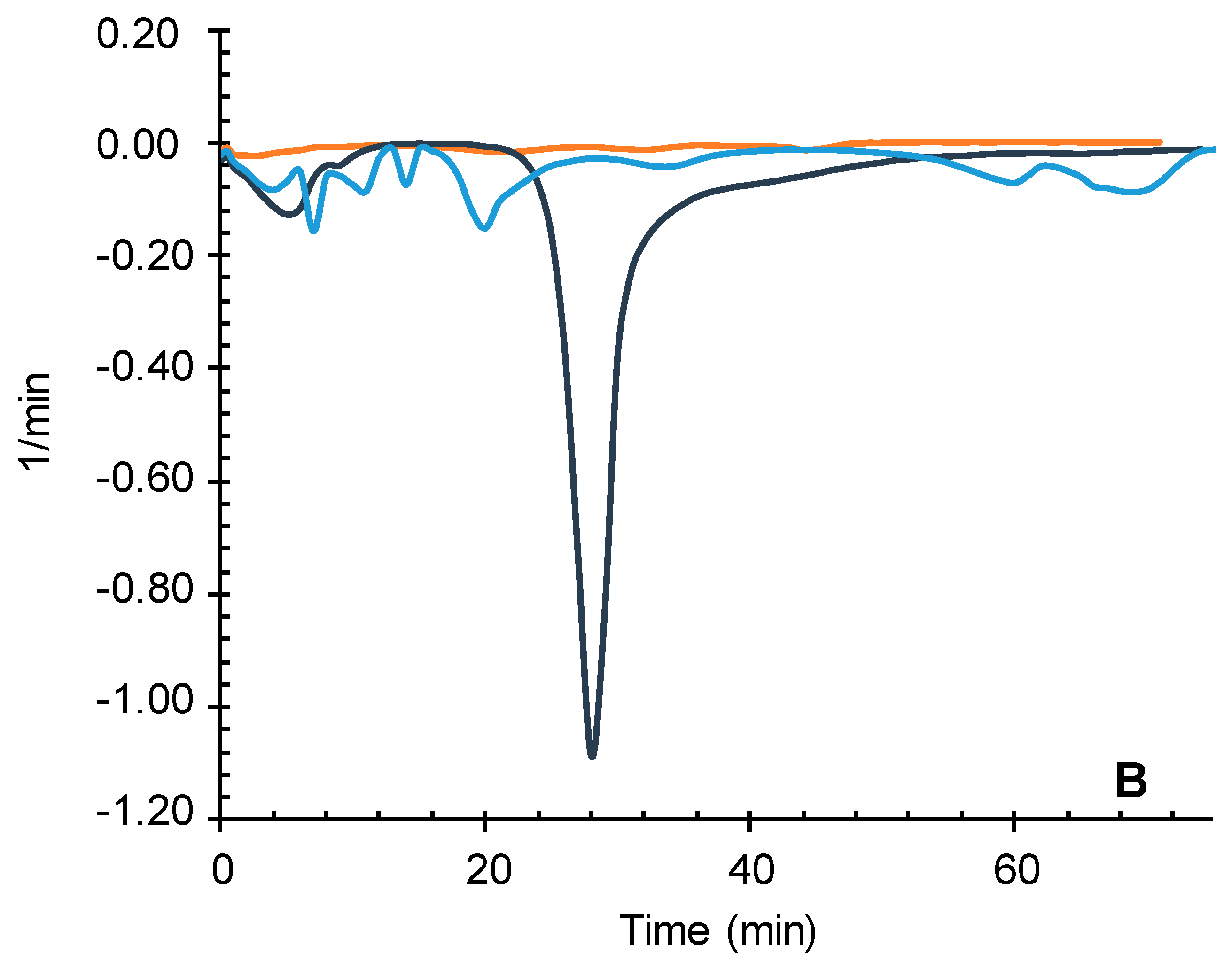
Figure 9.
DRX powder X-Ray Diffraction of Chitosan-Fe (Blue line) and Fe (Orange line).
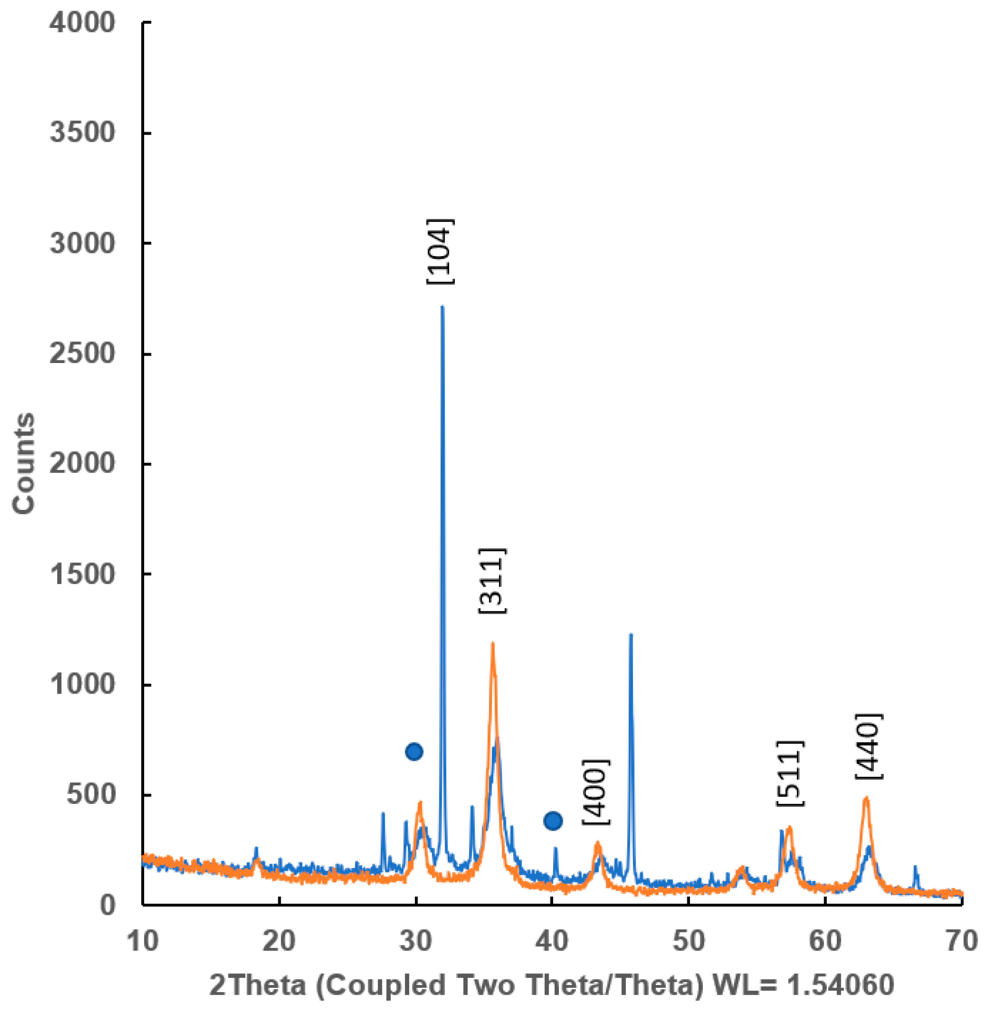
Figure 10.
IRTF of Chitosan (Grey line), Chitosan-Fe (Blue line) and Fe (Orange Line).
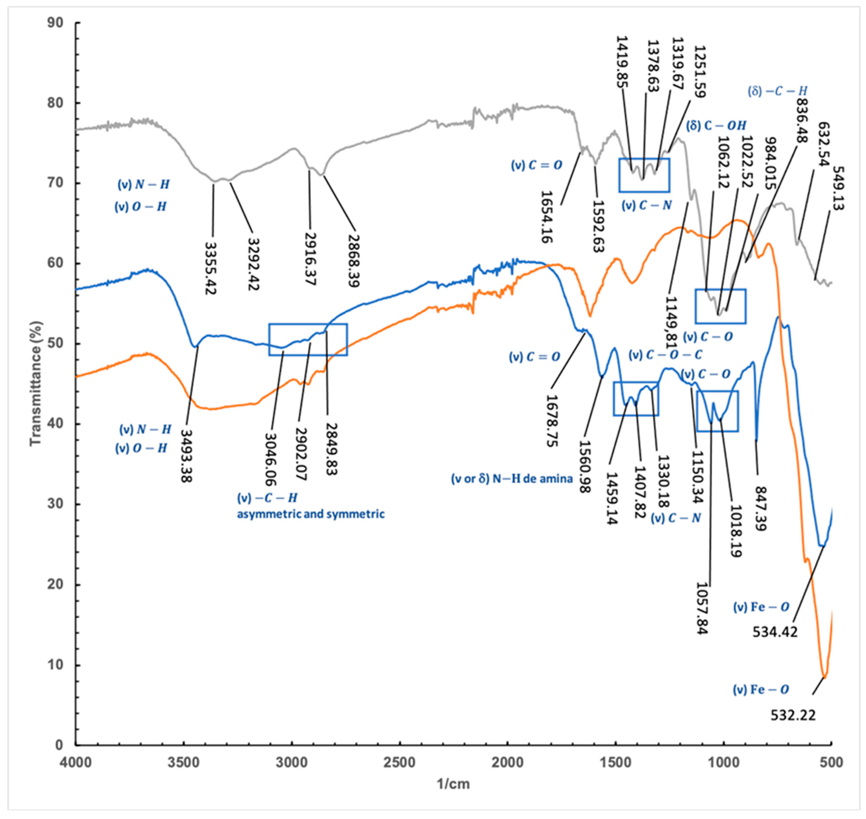
Figure 11.
A: Chitosan Polymer. B: Detail of small dark areas of the chitosan polymer.
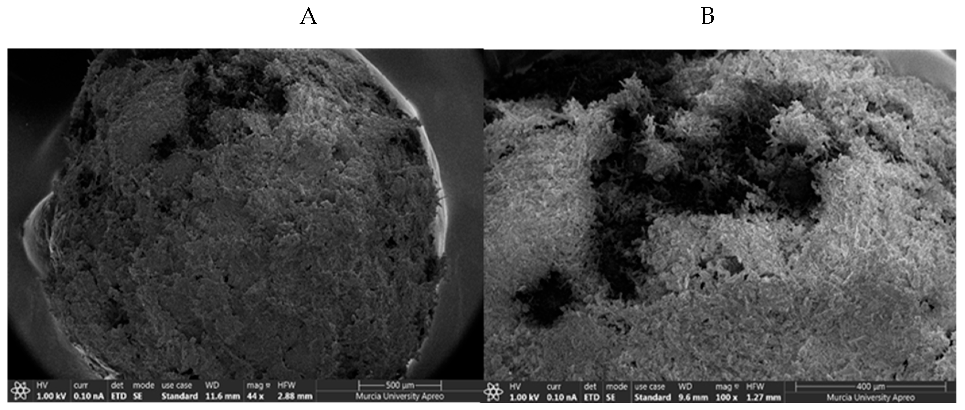
Figure 12.
EDX of Chitosan (A) and Chitosan-Fe (B).
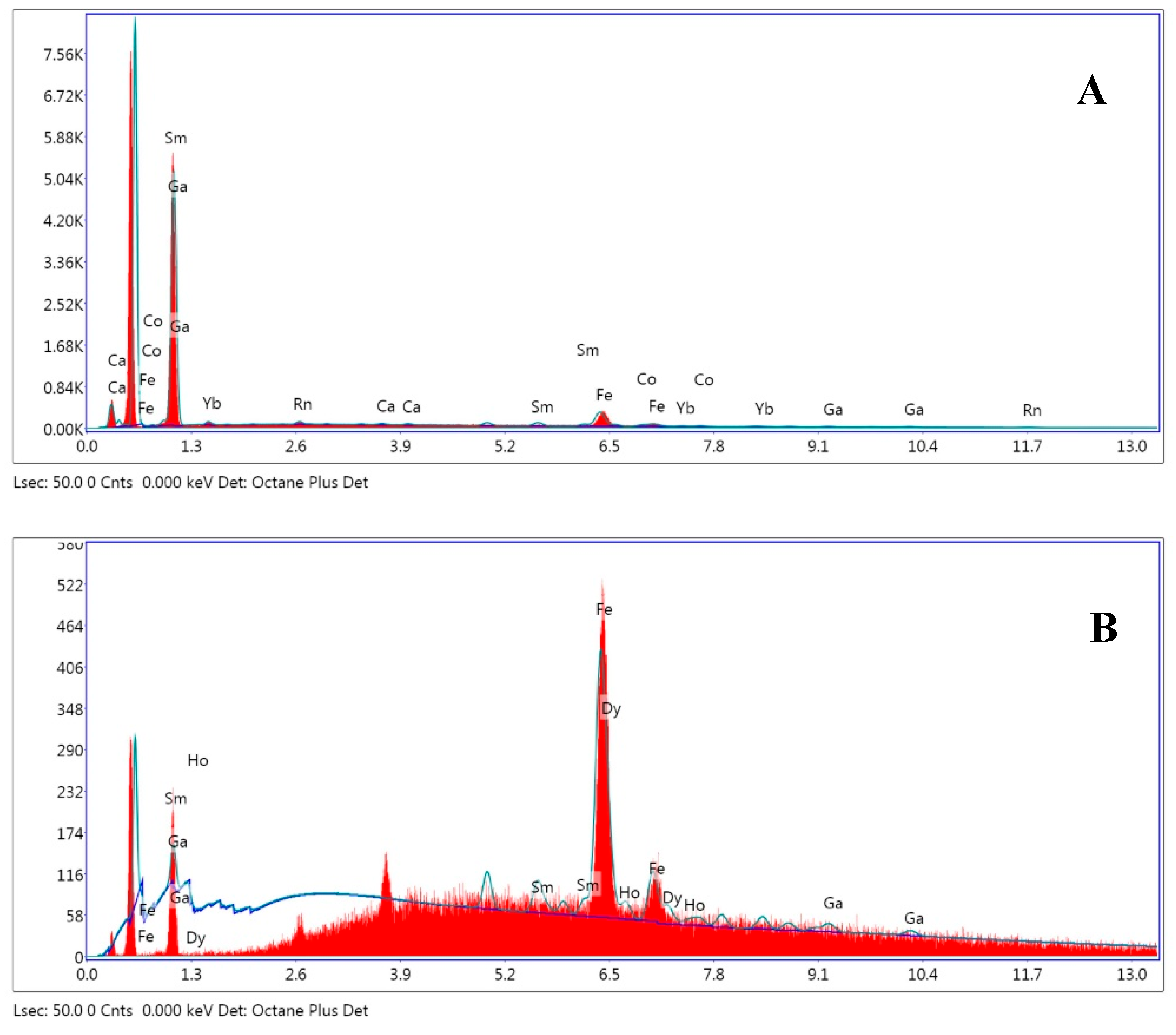
Figure 13.
Optimized Chitosan-Fe(II) model systems. Colour atom code: grey: carbon, red: oxygen, blue: nitrogen, cyan: iron.
Figure 13.
Optimized Chitosan-Fe(II) model systems. Colour atom code: grey: carbon, red: oxygen, blue: nitrogen, cyan: iron.
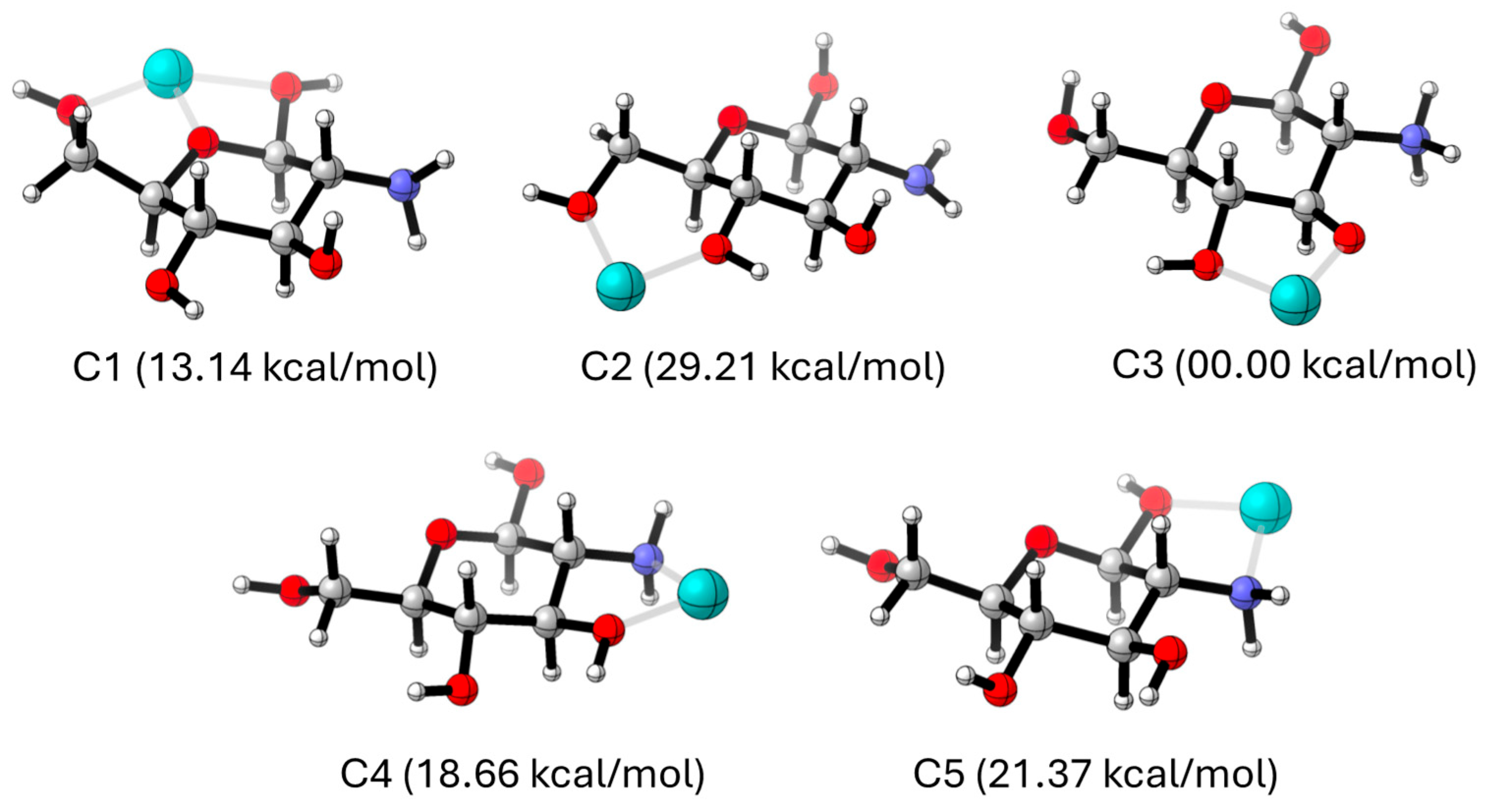

Table 1.
Kinetic Parameters for Adsorption of Direct Red 83:1 onto Chitosan Magnetic Polymer.
| PFOM 1 | Chitosan-Fe | |||
|---|---|---|---|---|
| C0 (mg/L) | qeexp | qecal | K1(min-1) | R2 |
| 50 | 2.27 | 1.05 | 0.033 | 0.987 |
| 100 | 4.69 | 3.11 | 0.040 | 0.881 |
| 150 | 6.97 | 5.31 | 0.031 | 0.960 |
| 200 | 8.60 | 9.36 | 0.027 | 0.950 |
| 300 | 12.47 | 18.29 | 0.029 | 0.772 |
| PSOM 2 | Chitosan-Fe | |||
| C0 (mg/L) | qeexp | qecal | K2(min-1) | R2 |
| 50 | 2.27 | 2.27 | - | 0.999 |
| 100 | 4.69 | 4.69 | - | 0.999 |
| 150 | 6.97 | 6.97 | - | 0.999 |
| 200 | 8.60 | 8.60 | - | 0.999 |
| 300 | 12.47 | 12.47 | - | 0.999 |
| IDM 3 | Chitosan-Fe | |||
| C0 (mg/L) | qeexp | qecal | Ki (mg/g min1/2) | R2 |
| 50 | 2.27 | 1.06 | 0.11 | 0.930 |
| 100 | 4.69 | 1.50 | 0.32 | 0.662 |
| 150 | 6.97 | 2.08 | 0.46 | 0.834 |
| 200 | 8.60 | 0.63 | 0.71 | 0.978 |
| 300 | 12.47 | -1.37 | 1.20 | 0.977 |
1 PFOM: Pseudo-first-order model; 2 PSOM: Pseudo-second-order model; 3 IDM: Intraparticle diffusion model.
Table 2.
Freundlich, Langmuir and Temkin parameters.
| Isotherm | Parameter | Chitosan-Fe |
|---|---|---|
| Freundlich | KF | 1.28 |
| nF | 1.68 | |
| R2 | 0.844 | |
| Langmuir | qmax | 17.46 |
| KL | 0.76 | |
| aL | 0.043 | |
| R2 | 0.884 | |
| RL | 0.13-0.024 | |
| Temkin | aT | 0.48 |
| bT | 0.67 | |
| R2 | 0.946 |
Disclaimer/Publisher’s Note: The statements, opinions and data contained in all publications are solely those of the individual author(s) and contributor(s) and not of MDPI and/or the editor(s). MDPI and/or the editor(s) disclaim responsibility for any injury to people or property resulting from any ideas, methods, instructions or products referred to in the content. |
© 2024 by the authors. Licensee MDPI, Basel, Switzerland. This article is an open access article distributed under the terms and conditions of the Creative Commons Attribution (CC BY) license (https://creativecommons.org/licenses/by/4.0/).
Copyright: This open access article is published under a Creative Commons CC BY 4.0 license, which permit the free download, distribution, and reuse, provided that the author and preprint are cited in any reuse.


