

Submitted:
11 March 2024
Posted:
13 March 2024
You are already at the latest version
Abstract
We give a series of numerical examples of competitive evolution in the predation system, showing in some cases how the choice is made to increase the efficiency of the predation mechanism (or other significant parameters) to the detriment of populations (both of prey and predators). We then develop the mathematical theory that enables us to understand the causality involved, and identify a trend towards the emergence of the functional predation mechanism as such (and not of populations of the species involved). The realization of this trend only takes place when the conditions for it are offered by the hazards proposed to successive competitive choices. The logical structure of this trend is similar to that of the « tendency of rate of profit to fall » in certain economic models.
Keywords:
predator–prey interactions
; hopf bifurcation
; limit cycle
; evolutionary trend
; evolutionary ecology
; emergence of efficiency
MSC: 92B05; 92D40; 92D25; 34D20; 92D15
1. Introduction
It is well known that the causality involved in predation is highly complex, and difficult to reconcile with general trends such as "survival of the fittest". Indeed, if we have predators feeding on prey, it is clear that, from a demographic point of view, the presence of predators is always detrimental to the prey, whereas, from the predators' viewpoint the consumption of prey is necessary for their survival, but, if excessive, it leads to a scarcity of prey, which in turn leads to predator starvation. Clearly, moderation of the predation mechanism is fundamental to its stability, and perhaps to its long-term viability (you can't kill the goose that lays the golden eggs ...). It is also clear that time must play an explicit role in any causal description of these mechanisms.
The predator-prey system of population dynamics, of which there are several models, makes it possible to explain the various possible situations and to understand their causality, and above all, by placing two predators in competition, to understand the reasons for the evolutionary choices that follow.
But, on the other hand, a more complete system, known as predation-commensalism, is a model of the global economy that enables us to proof certain properties of the latter, notably TRPF (Tendency of Rate of Profit to Fall), which simply results from the competition between various firms which, in order to increase their market share, reduce their profit margins. The consequence of TRPF is the pursuit of innovation and technological progress, which is precisely what allows the rate of profit to be reduced. (See [1] chap 9 and in particular section 9.3). In this paper, we follow an analogous approach in the predator-prey system to identify the natural tendency resulting from repeated competitive evolution. Under plausible hypotheses (see section 4), it appears that the natural tendency of this system is to increase its own efficiency. Clearly, this does not always correspond to the demographic growth of the predator, and may even lead to its disappearance. This is a "tendency", a kind of "vocation" that only comes to fruition when the conditions for its realization are offered by the hazards of successive competitive evolutions (just as TRPF does not automatically lead to technological progress). It is nevertheless clear that the loss of efficiency is rejected by competitive evolution, which nonetheless accepts drastic population reductions (of predators and prey) under certain conditions.
Let's take a predation model for two species (of populations x and y, prey and predator respectively),
where x'=f(x) is the equation for prey evolution in the absence of predators, for which we take the logistic equation:
(a is the natural growth rate of x and P the environmental carrying capacity).
The functional response h(x) is taken from Holling's type-II, in the form
Remark: This predation function h(x) is essentially analogous to the widely used Holling type-II functional response, (see for instance [1,2,3] or one of Holling's original articles [4]). Holling's type-II functional response resembles type-I for small x, but then gradually tends towards a constant (representing the predator's satiety). However, here we use the hyperbolic tangent, ℎ(𝑥)=𝑏𝑇𝑎𝑛ℎ(𝑒𝑥/𝑏), instead of the algebraic Holling type-II form, ℎ(𝑥)=𝑏(𝑒𝑥)/(𝑏+𝑒𝑥). Indeed, the hyperbolic tangent expresses the idea of proportionality capped by satiety much better than the algebraic expression. It often enables us to better understand the respective roles of proportionality for small x (chance encounters) and the satiety ceiling.
Within the framework of this model, there are six significant parameters: c (death rate of predators in the absence of prey), e (efficiency of the predation mechanism), b (satiety ceiling of predators), τ (conversion rate of consumed prey into predator population), a (natural growth rate of prey in the absence of predators and abundance of resources) and P (carrying capacity of the environment, i. e. population of preys alone that it can admit). The last two concern only the behavior of prey with their own resources. The first four concern the behavior of predators and their relationship with prey.
The parameters are fixed in all numerical simulations and are given by:
a=1.0, P=4.0, b=1, c=0.7616
Note that we can always take τ=1 by choosing appropriate units to measure the populations of x and y (the unit of y is the quantity of predators obtained by consuming a unit of x). We will always do so, except in cases where we need to compare several predators with different conversion rates, where a single choice is not possible.
The solutions and attractors in system (1) have different properties depending on the parameter values. It is useful to bear these in mind before tackling the problem of competition between two predators.
Apart from the (0,0) and (P,0) which are always equilibria, to find the equilibrium (x0,y0) internal to the domain of definition x > 0, y > 0, simply solve system (1) with the first members replaced by 0. From the second equation we have Eq. (5) below and then from the first we get Eq. (6):
It is well known that, depending on the parameter values, this equilibrium may or may not be stable. In the latter case, the attractor is a periodic cycle surrounding the equilibrium point. It is worth recalling here the evolution of the equilibrium point and this attractor as a function of the parameter e when the other parameters are fixed. Indeed, we shall see that the variation of e implies particularly significant qualitative properties. We shall also see (section 4) that variations in e play a key role in the dynamics of evolution.
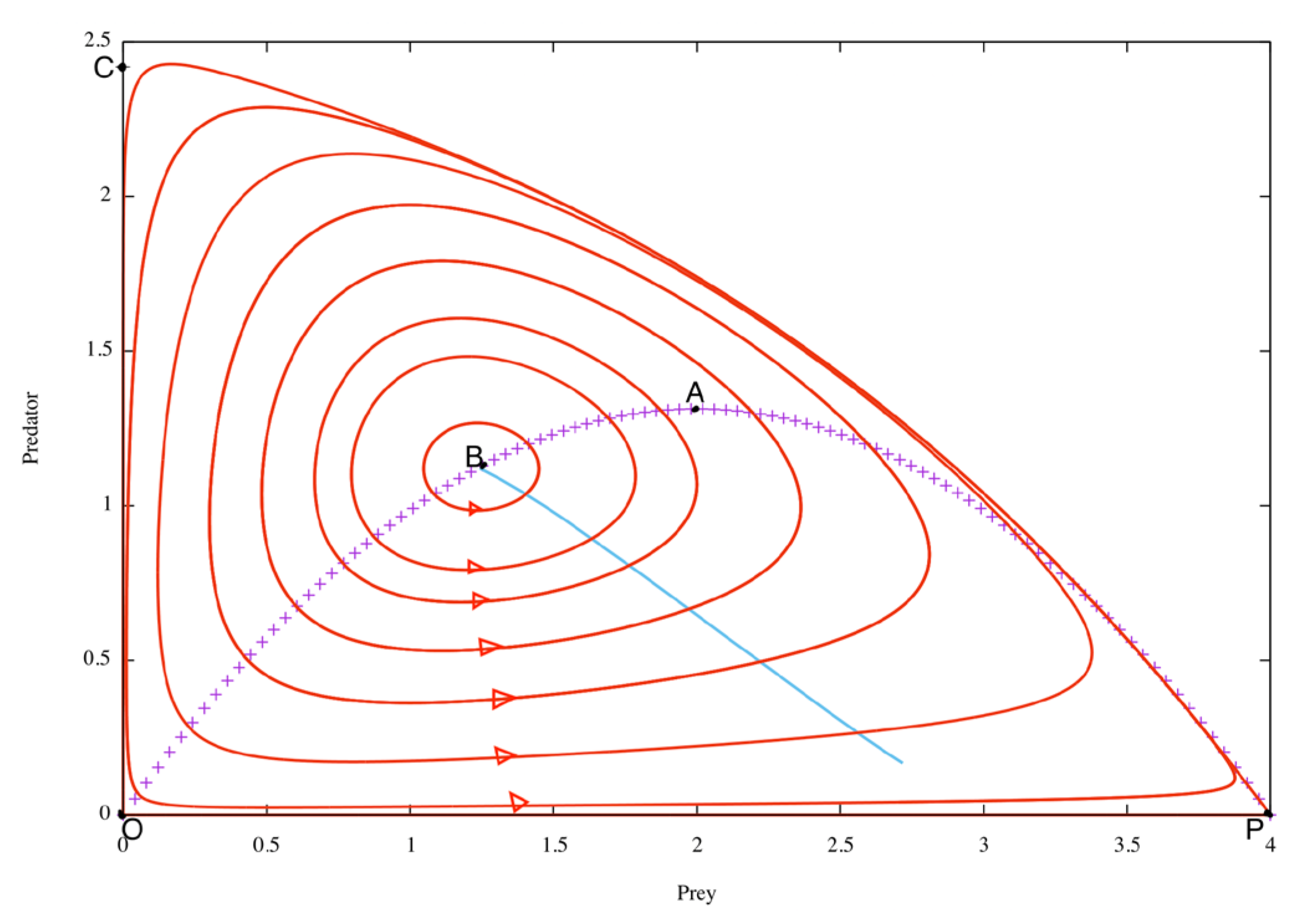
By fixing the values of the other parameters and varying e, we can easily see (see also [5] or [1] chap 6) thanks to Eq. (5) and (6) with Eqs.(2)-(3), that the equilibrium point (x0,y0) moves along an arc of a parabola (see Figure 1) which contains the two equilibria (0,0) and (P,0) of the prey alone, i.e. in the absence of predator, (which therefore always exist independently of e). This parabola arc is traversed in the direction of decreasing x0 for increasing e. According to Eq. (6), the internal equilibrium point exists for f(x0 )>0, which is equivalent to x0<P. The corresponding value of e is the viability threshold of predation. For increasing e, the equilibrium point moves along the parabola, rising towards the apex A (top of the parabola) and then falling towards the origin, which corresponds to e = +∞. The arc of the parabola between P and A is the normal mode (as e increases, the equilibrium population of prey decreases and that of predators increases). For larger values of e, we are in the paradoxical region (between A and O; when the efficiency e increases, both equilibrium populations of prey and predators decrease).
The stability of the internal equilibrium point (x0,y0) depends on e, and therefore on its position along the parabola. It is stable from P (i.e. for small e) up to a certain point B in the paradoxical region, Figure 1, where there is a PAH bifurcation (= Poincaré-Andronov-Hopf, often referred to as Hopf bifurcation, see for example [6,7]). Equilibrium still exists in the BO arc, but it is unstable, the attractor being a periodic cycle surrounding the equilibrium point. This cycle naturally depends on e; we have drawn it on Figure 1 for several values of e. The literature is very rich on these problems of equilibria, cycles, see for example [8,9,10,11] and references therein cited.
It should be pointed out that this general pattern naturally depends on the parameter values. It is easy to see (see [1] section 6.5) that the bifurcation of PAH is due to the capping of satiety, (parameter b). As b increases, the PAH bifurcation moves towards the origin, and for b=+∞ it coincides with the origin; in other words, for b=+∞ (which is equivalent to h(x)=e x), there is no PAH bifurcation and the equilibrium is always stable (it is the attractor).
It is useful to calculate, for each value of e beyond the PAH bifurcation, the average values of the densities of x(t) and y(t), along the corresponding cycle, which we will denote by , . They differ from (x0,y0), and describe (see Figure 1) a curve that is virtually rectilinear starting from the PAH bifurcation and moving for increasing e with increasing and decreasing .
The shape of the cycles is very interesting. For values of e slightly above the PAH bifurcation, it is a small, approximately elliptical cycle surrounding the equilibrium point. But for larger e, the cycle gradually adopts a vaguely triangular shape, which becomes, for larger e, practically a curvilinear triangle with smooth (rounded) vertices, whose sides are the x and y axes and a curve arising from (P, 0) solution of the limit system for e = +∞ (which is equivalent to taking h(x)=b) and whose vertices are the two equilibria of the prey alone, O and P, and a point C.
This highly significant geometry is known as the HNR triangle (for Hubris - Nemesis - Resilience). In fact, as we go through the cycle as a function of t, the curvilinear side close to PC is an increase in the predator population at the expense of the prey population, due to the hubris of e efficiency. Arriving near C, there are very few preys and many predators, leading to a rapid decline in the predator population, which almost vanishes out of food; this is the CO side (nemesis = punishment for hubris). At the approach of O, there are very few predators and preys, so they can proliferate unhindered by predators, which is what makes the side close to OP (close to the evolution of preys alone, it's prey resilience). This closes the cycle, which begins again periodically.
Figure 1.
Shows the limit cycles exhibited by the system, for e ranging from 6 to 30, with increasing amplitude as the parameter e increases. The fixed points of the system for different values of e, with all other parameters fixed as given by Eq. (4), are represented by the arc of the parabola with vertex A (cross-shaped line). The almost rectilinear curve starting from B is the curve of means values (, ).
Figure 1.
Shows the limit cycles exhibited by the system, for e ranging from 6 to 30, with increasing amplitude as the parameter e increases. The fixed points of the system for different values of e, with all other parameters fixed as given by Eq. (4), are represented by the arc of the parabola with vertex A (cross-shaped line). The almost rectilinear curve starting from B is the curve of means values (, ).
But we can go further in describing the structure of HNR cycles for very large e: for large enough e, the cycle is very close to the curvilinear triangle. This is formed by the axes and the solution of the limit system for e=+∞ (which consists in replacing Tanh by 1) starting from the equilibrium of prey alone, (P,0). This solution, which is the hubris phase, intersects the y-axis with a non-zero x' velocity (because of Tanh=1), so that there is a matching (boundary layer for very large e) to match the y-axis (the nemesis phase). This matching occurs fairly quickly and is very different from the vertices (0, 0) and (P, 0), which are points of equilibrium, so that passing near them the movement is very slow for large e, unlike passing near the top vertex, which is a matching (= sudden change of direction without slowing down for large e).
For very high values of e, by inspection of the solutions x(t) and y(t), we observe that the period (which must tend towards infinity because of the slowdowns mentioned) appears to be proportional to e.
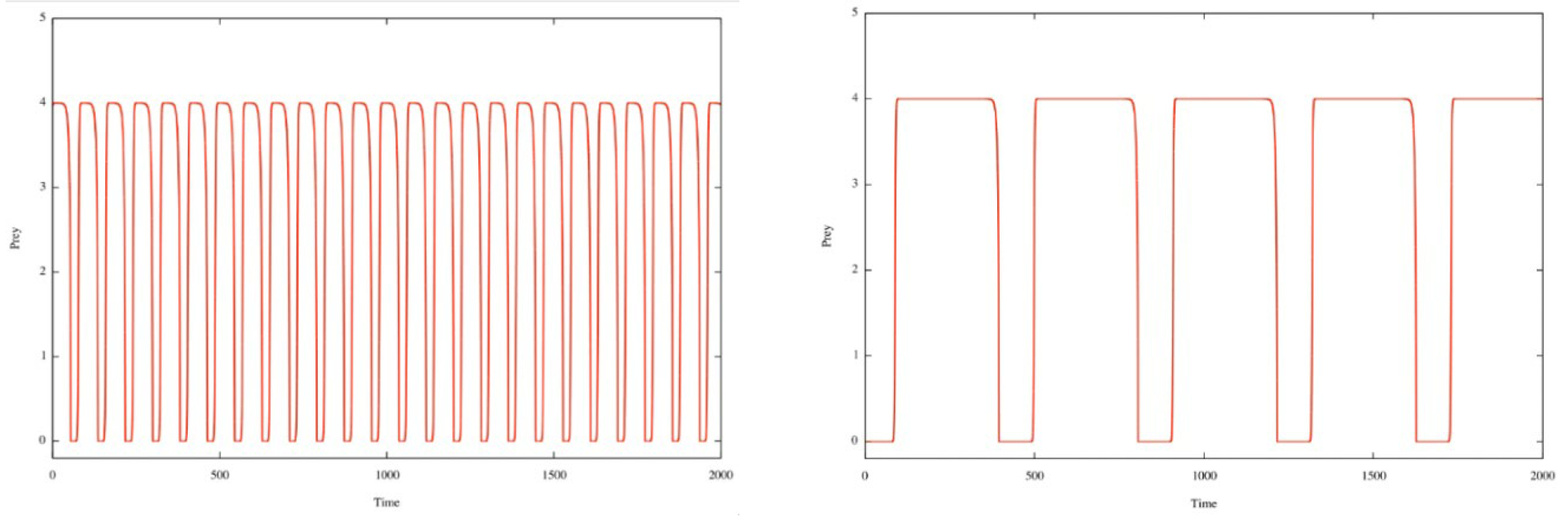
In the behavior of x(t) we observe the presence of two levels, close to 0 and P (corresponding to the slowdowns of the passages near the equilibrium points (0, 0) and (P, 0). See the two figures below for e=6 and e=30.
Figure 2.
The temporal series x(t) for e=6 and e=30, the other parameters are given by Eq. (4).
The behavior of y(t) is similar, except that the two stages merge, as y(t) values are practically zero for the two passages near (0, 0) and (P, 0) and the arc of orbit that connects them. In fact, all that remains in each cycle is the rapid rise and fall of y(t) (hubris and nemesis). In other words, the periodic function y(t) becomes a kind of pulse (always the same regardless of e) increasingly spaced out in time as e→+∞. See the two figures below for e = 6 and e = 30.
Figure 3.
The temporal series y(t) for e=6 and e=30, the other parameters are given by Eq. (4).
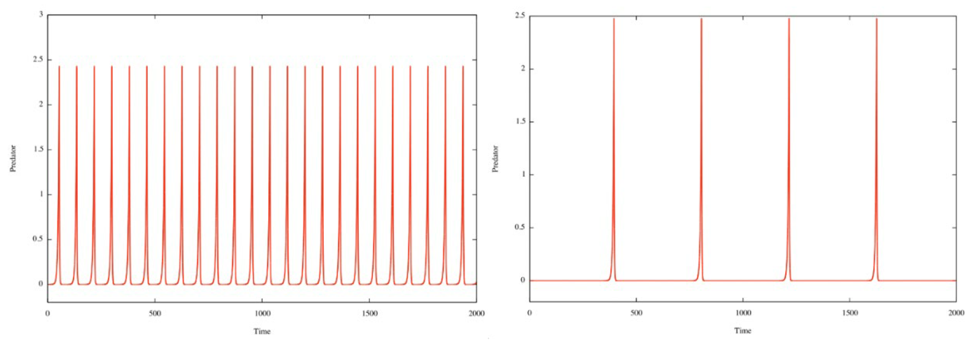
Taken together, the four figures above perfectly explain the almost rectilinear shape of the curve of mean values (, of the densities of x(t) and y(t) along the corresponding cycle, as a function of e (see Figure 1). Indeed, as e tends to infinity, tends to zero and tends to a positive constant.
Another important point for understanding the sequel is that the unknown x0 is given by the second equation of system (1), which is that of predator functioning (x0 is the prey population that keeps the predators in equilibrium); x0 is therefore independent of a and P. This remarkable property is at the root of the understanding of certain aspects of the paradoxes considered in the sequel.
Later (section 6), we'll introduce slightly more complex systems, known as predation-commensalism, to deal with specific questions.
It should also be noted that the mathematical properties encountered are to be taken as tendencies and not as exact results. This is the case for all properties established with the help of models; in particular here, when e→+∞, the model becomes inoperative because there are populations that are too small at certain instants, so that the very concept of population disappears.
We shall see that these elements are important for correctly interpreting the causality and implications of the choices made by evolution.
2. Evolution Chooses to Increase the Efficiency of the Predation Mechanism
In this section we consider four numerical examples of competition between two predators of different efficiencies in different regions (normal, paradoxical, cyclic attractors).
We consider a population x of prey and two populations y1 and y2 of predators, modeled by the system,
where are given by expressions like (2) and (3) with indices 1 and 2. The values of the parameters (except e1 and e2) are equal for both predators:
In the numerical computations in this section, and almost everywhere in this article, the starting point is taken close to the attractor of x and alone, to highlight the displacement of the attractor in competition with (if we start from another point, the final behavior is obviously the same, however, this initial condition must be chosen sufficiently close to the attractor to avoid the transient part which would distort the comparison with the attractor of x and alone. On the other hand, the attractor of x and alone is easily found by making .
Numerical example -1- : in the normal region
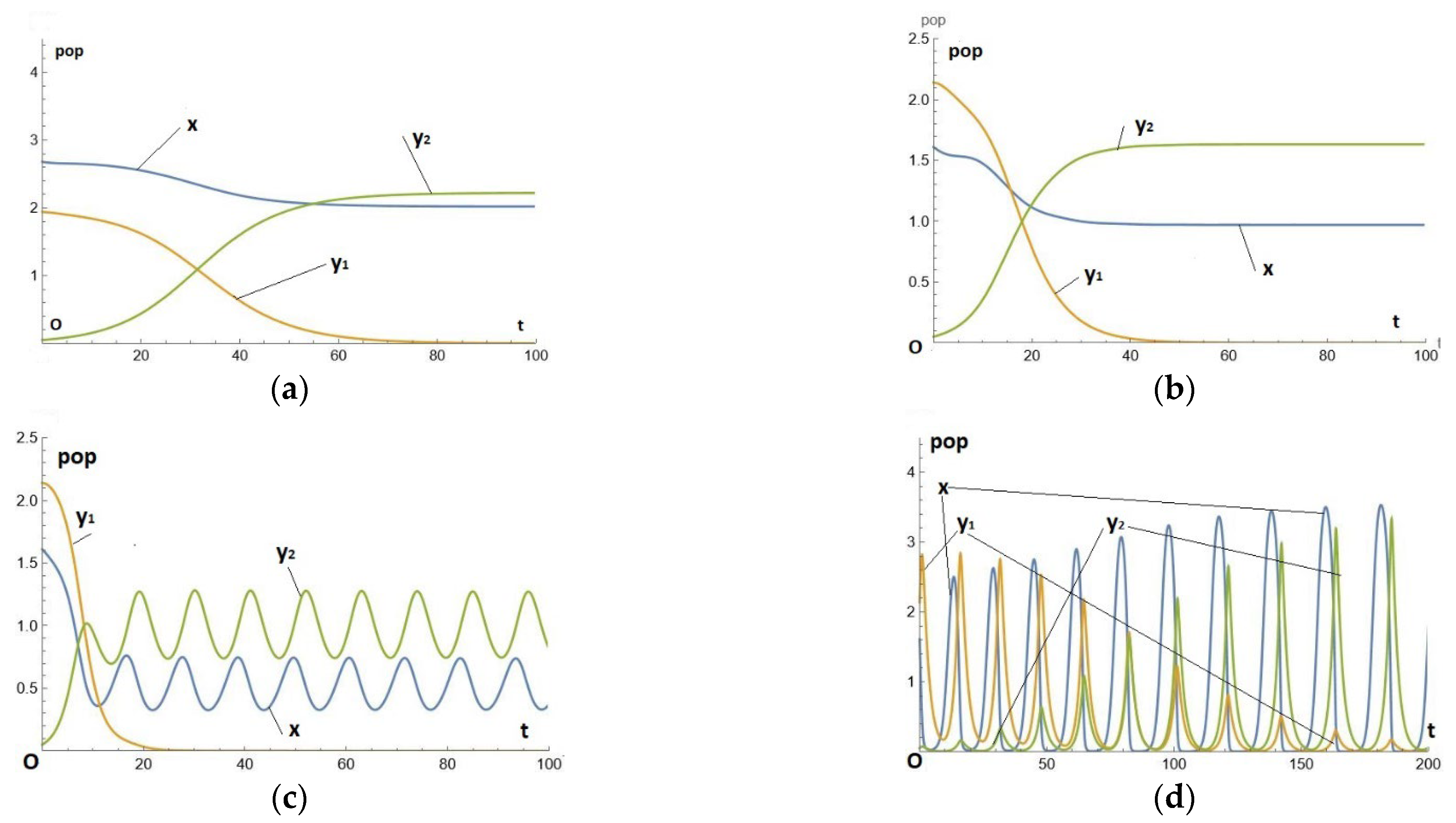
We take , so the two predators differ only in efficiency (that of being greater than that of ). It is easy to check that they are both in the normal region (arc of the parabola between P and A: as e increases, the equilibrium population of prey decreases and that of predators increases). We then calculate the solution of Eq. (7) starting from initial values such that x(0) and are very close to the equilibrium position of the system without , indeed we start from the initial condition (2.68,1.94, 0.05). The numerical solution is shown in Figure 2(a).
Unsurprisingly, the initial predator is replaced by the more efficient predator. This is accompanied by a decrease in the prey population and an increase in the predator population (the final population of is greater than the initial population of ).
Note that, starting from any other initial position, the final result is the same (this is the attractor), but initially there is a transient regime, an oscillation, since we are not starting from an equilibrium position.
Numerical example -2- : in the paradoxical region
We take (it's easy to check that they are both in the paradoxical region). Starting from the initial condition (1.61, 2.13, 0.05). The numerical solution is then shown in Figure 2(b).
We can see that the initial predator is always replaced by the more efficient . This is accompanied by a reduction in the prey population and also a reduction in the predator population (the final population is smaller than the initial population).
Competitive evolution in the paradoxical region is therefore moving towards an increase in the efficiency of the predation mechanism, to the detriment of both predator and prey populations.
Numerical example -3- : in the paradoxical region, slightly beyond the bifurcation of PAH
We take (the predator is the same as in the previous example, but is more efficient, having passed the bifurcation, which takes place around = 0.93). Starting from the initial condition (1.61, 2.13, 0.05), the numerical solution is shown in Figure 2(c). As in the previous example, competitive evolution leads to an increase in the efficiency of the predation mechanism, to the detriment of both predator and prey populations. But the final state is oscillating, this is the cyclic attractor of the system in (x,).
Numerical example -4- :andfar beyond the bifurcation of PAH
We take (both predators have much greater efficiencies than the bifurcation, which is at e=0.93 approximately). Starting from the initial condition (1.6, 2.1, 0.05) the numerical solution is shown in Figure 2(d).
This result lies in the region of large cycles, which are only known by numerical computation, making it all the more difficult to interpret the results, or at least to draw general statements from them. The predator is always replaced by a more efficient one. The prey population is visibly increasing; the predator population also seems to be increasing in the higher values, but the peaks are more widely spaced, so that the average values over the period are smaller, in line with the Figure 1.
Figure 2.
The temporal series, x(t), (t) for the parameters given by Eq. (8), (a): in the normal region, , and the initial condition (2.68,1.94, 0.05), (b): in the paradoxical region, and the initial condition (1.61, 2.13, 0.05), (c): in the normal region, , and the initial condition (1.61, 2.13, 0.05), (d): in the paradoxical region, and the initial condition (1.6, 2.1, 0.05).
Figure 2.
The temporal series, x(t), (t) for the parameters given by Eq. (8), (a): in the normal region, , and the initial condition (2.68,1.94, 0.05), (b): in the paradoxical region, and the initial condition (1.61, 2.13, 0.05), (c): in the normal region, , and the initial condition (1.61, 2.13, 0.05), (d): in the paradoxical region, and the initial condition (1.6, 2.1, 0.05).
It thus appears (on the basis of these numerical computations) that, all other parameters being the same, evolution always chooses to increase the efficiency e, which is not necessarily accompanied by a demographic boom in predators (their population decreases in the paradoxical region). This result is highly significant, as it seems to indicate that, as opportunities arise, the natural tendency of evolution is to increase the efficiency of the predation mechanism. If these opportunities arise repeatedly, the process eventually leads to HNR cycles, and even eventually to the disappearance of the mechanism as such, as the model fails for very small populations.
3. Theory of Competitive Evolution in the Predatory System
System (7) is in the framework of systems of the form,
The equilibrium points inside the positive octant (i.e. with the three strictly positive coordinates) are the solutions of the system (10) below which contains two equations with the single unknown x:
It follows that, generically, there is no equilibrium point inside the octant and the point attractors are on the boundary. Of course, there may be non-point attractors, and we will see examples of this (numerical example -5-). For the solutions of (9), let us calculate the expression:
As the populations are positive, this shows that, at each point, the vector field passes through the constant plane towards the or axis, depending on whether is larger or smaller than at that point.
In the special case of system (7) with (2) and (3), we have
so that competition between two predator species only concerns the significant parameters c, e, b, τ. This expression enjoys the remarkable property of being increasing with respect to each of the parameters e, b, τ and decreasing with respect to c, independently of the point x, (this is obvious for c, e, τ; for b too, with a simple calculation, or by thinking of its role as a satiety ceiling). This result is summarized in the proposition below.
Proposition 1.
Consider system (7) in the case where the difference between the two attractors concerns only one of the parameters c, e, b, τ. Then the attractor is necessarily in one of the planes with coordinates (x, or (x,, precisely the one with the largest (resp. smallest) value of the parameter concerned, if this is one of the b, e, τ (resp. c).
It is worth noting that this proposition, which may seem obvious from a Darwinian perspective, is rigorously true, concerning attractors of both a punctual or not nature (cyclic, in particular) and is nevertheless perfectly compatible with the paradox pointed out in section 2, which concerns the parameter (the attractor is therefore in the (x,-plane) and where the equilibrium populations are smaller for (x, than for (x,.
On the other hand, if we modify two (or more) of the significant parameters, the value of is no longer necessarily the same everywhere, it may depend on x, and we can only derive local results from (12).
So, for example, let (x0,y10) be a stable equilibrium point of the system for x and alone. Then, the point (0, x0,y10) is automatically an equilibrium point of the three-dimensional system; its local stability is given by that of the linearized system (Jacobian matrix at the point (x0, y10 ,0) ). It has two negative real eigenvalues (corresponding to the restriction to , so this point is three-dimensionally locally stable or not, depending on whether the eigenvalue corresponding to the transverse eigenvector is negative or positive (it is necessarily real). We can see from the third equation (9) that transverse stability may or may not hold, depending on whether is negative or positive. Now, since (x0,y10) is an equilibrium point of the system in the (x,y1)-plane, we have (see second equation (10)) . So, we have stability if,
or instability if the sign is >. This result is summarized in the proposition below.
Proposition 2.
Let (x0,y10) be a stable equilibrium point of the system for (x,y1) alone. Then the point (x,y1,0) is a three-dimensional attractor if (13) is satisfied, and is transversely unstable if (13) with sign > is satisfied. A similar result holds for a stable equilibrium in the (x,y2)-plane.
We have an analogous result in the case of a cyclic attractor 𝝘 of the system for (x,y1) alone, replacing q by its integral along 𝝘. Let (x0(t),y10(t)) be the parametric representation of 𝝘 as a function of time. From the first two equations (10) we have,
(which is the analogue of above). The variational equation of (10) with respect to in (3.1) gives:
So that stability amounts to,
This result is summarized in the proposition below.
Proposition 3.
Let (x0(t),y10(t)) be the parametric representation a cyclic attractor of the system for (x,y1) alone. Then it is also a three-dimensional attractor if (16) is satisfied, and it is transversely unstable if we have (16) with the sign > instead of <. A similar result holds for a stable equilibrium in the (x,y2)-plane.
Naturally, Propositions 2 and 3 hold in the framework of the local theory of differential equations (whereas system (9) is perfectly general). Specific examples can be found by numerical computations.
4. General Comment. The choice of Evolution as a Functional Vocation
Finally, it is easy to get a synthetic idea of the (often paradoxical) behavior of competition between two predators by taking the following two elements into account:
-i- The dynamics of the system with regard to competition between and is given by equation (11) (and the analogue by exchanging indices 1 and 2), which we reproduce here in a slightly different form:
which holds true for all positive x,
-ii- Of the significant parameters of this predation model, e, b, τ, c, a, P, only e, b, τ, c, are involved in (17). The other two, a,P, are not involved, as they relate to prey behavior. The expression q is increasing with respect to e,τ, and b (for the latter this results from its meaning as a predation ceiling, or from a little calculation) and decreasing with respect to c.
Let's consider the case where only one of the parameters e,τ,b and c is different for the two attractors. Expression (17) has constant sign everywhere, so the attractor (whatever its nature, point-like or not) is necessarily on one of the coordinate planes (x,y1) or (x,y2), the one corresponding to the larger e,b,τ or the smaller c. This is elementary Darwinism, as long as we interpret "advantage" and "disadvantage" in the sense of larger or smaller q and not the predator population or anything else large or small. The same applies when there are several parameters with different values, provided that the differences in the values of these parameters are all in the same direction of increasing or decreasing q (examples: increasing τ and b, or decreasing e and increasing c).
On the other hand, if several of the parameters e,τ,b and c are different for the two predators, and the differences in the values of these parameters produce variations of various signs on q, the sign of the right hand term in (17) may be different for different values of x, making it possible for a cyclic attractor to exist inside the positive octant (orbit returning to the starting point, see for instance the numerical example -5- hereafter). The attractor can then lie on one of the coordinate planes or inside the positive octant. Note in any case that there can be no point attractor outside the coordinate planes, as we pointed out in connection with Eq. (10).
It is useful to return to the extremely simple case where only one of the significant parameters e,τ,b and c is varied. We can say that the predation mechanism has a tendency (or vocation) to increase e,τ,b and decrease c. This statement should be understood in the sense that, if it is proposed to the choice of evolution a variation in just one of these parameters, the competition will result in a choice of the highest (resp. lowest) value of e,τ,b (resp. c). This corresponds to the meaning of the terms tendency, vocation (and even to the term wish) in common parlance: a volitional agent can have one or several vocations, which means that, given the opportunity, he will choose to follow each of these vocations if the others are not affected, whereas a proposition implementing several vocations of opposite tendencies can have diverse outcomes (think of a person with artistic and welfare vocations, who has to choose between a "standard" job and a more artistic but less well-paid one).
This approach to interpreting results can be taken much further. If the choice of evolution is proposed repeatedly, always involving variations in just one of the parameters e,τ,b,c, it will systematically result in an increase in e,τ,b, or a decrease in c (proposals of opposite sign being rejected). This may seem natural and trivial, but we must realize that these trends or vocations do not always go in the direction of the predator's demographic boom, as the paradoxical examples show.
Now, if we think of the biological interpretation of the predation system, we can imagine that, in certain cases, τ,b,c depend on the physiological properties of the predator, whereas e depends on the ethological properties of the predator in its relationship with the prey and the environment. It is therefore natural to consider e as much more subject to the vagaries of evolution than τ,b,c. This makes the problem we are dealing with particularly interesting when only e is subject to variation. And it is precisely the variation of e with the other fixed parameters that reveals the paradoxical region and bifurcation of PAH developed in section 1.
We saw the special role of the parameter e and the interest in increasing it over time. It's easy to make a non-autonomous example, with slowly varying, increasing e-efficiency. As the variation is slow, the solution is practically quasi-static, so that at each instant we practically have the attractor for the corresponding value of e. For this purpose, we always use system (1)-(2)-(3) with,
a=1.0, P=4.0, b=0.53, c=0.43, τ1=1.0
and efficiency, e1=0.145+εt, ε = 0.0008,
with time t varying from 0 to 1000. We start from an initial condition close to the equilibrium of the preys alone. The solution is shown in Figs. 3(a-b). Note that the non-autonomous system with e1=0.145+εt can be transformed into an autonomous system with the new unknown e and the new equation e'=ε, which highlights the fast and slow dynamics if ε is small enough,
Figure 3.
Solutions of system (1)-(2)-(3), for the parameters given by a=1.0, P=4.0, b=0.53, c=0.43, τ1=1.0 and efficiency e1=0.145+εt, where ε = 0.0008, with time t varying from 0 to 1000. We start from an initial condition close to the equilibrium of the preys alone:. (a): temporal series x(t) and y(t), (b): the orbit in (x,y)-plane, (c): parametric representation of the solution in space (t,x,y) of the natural evolution of a predation mechanism whose efficiency is subject to evolutionary choice.
Figure 3.
Solutions of system (1)-(2)-(3), for the parameters given by a=1.0, P=4.0, b=0.53, c=0.43, τ1=1.0 and efficiency e1=0.145+εt, where ε = 0.0008, with time t varying from 0 to 1000. We start from an initial condition close to the equilibrium of the preys alone:. (a): temporal series x(t) and y(t), (b): the orbit in (x,y)-plane, (c): parametric representation of the solution in space (t,x,y) of the natural evolution of a predation mechanism whose efficiency is subject to evolutionary choice.
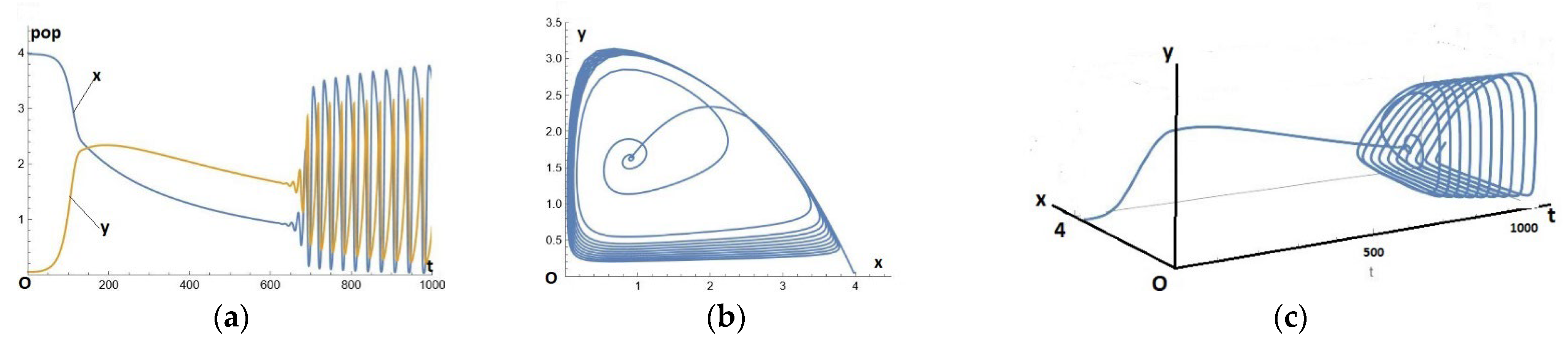
This can be compared with Figure 1 in section 1, identifying initially a non-paradoxical behavior, which becomes paradoxical after passing through the apex A (vertex of the parabola). Then appears the PAH bifurcation and the dilating cycles adopting the HNR gait.
We can also make a parametric representation in space, Figure 3(c), which can thus be seen as a symbolic vision (or artist's view) of the natural evolution of a predation mechanism whose efficiency is subject to evolutionary choice, which accepts (resp. refuses) the positive (resp. negative) variations that chance submits to it.
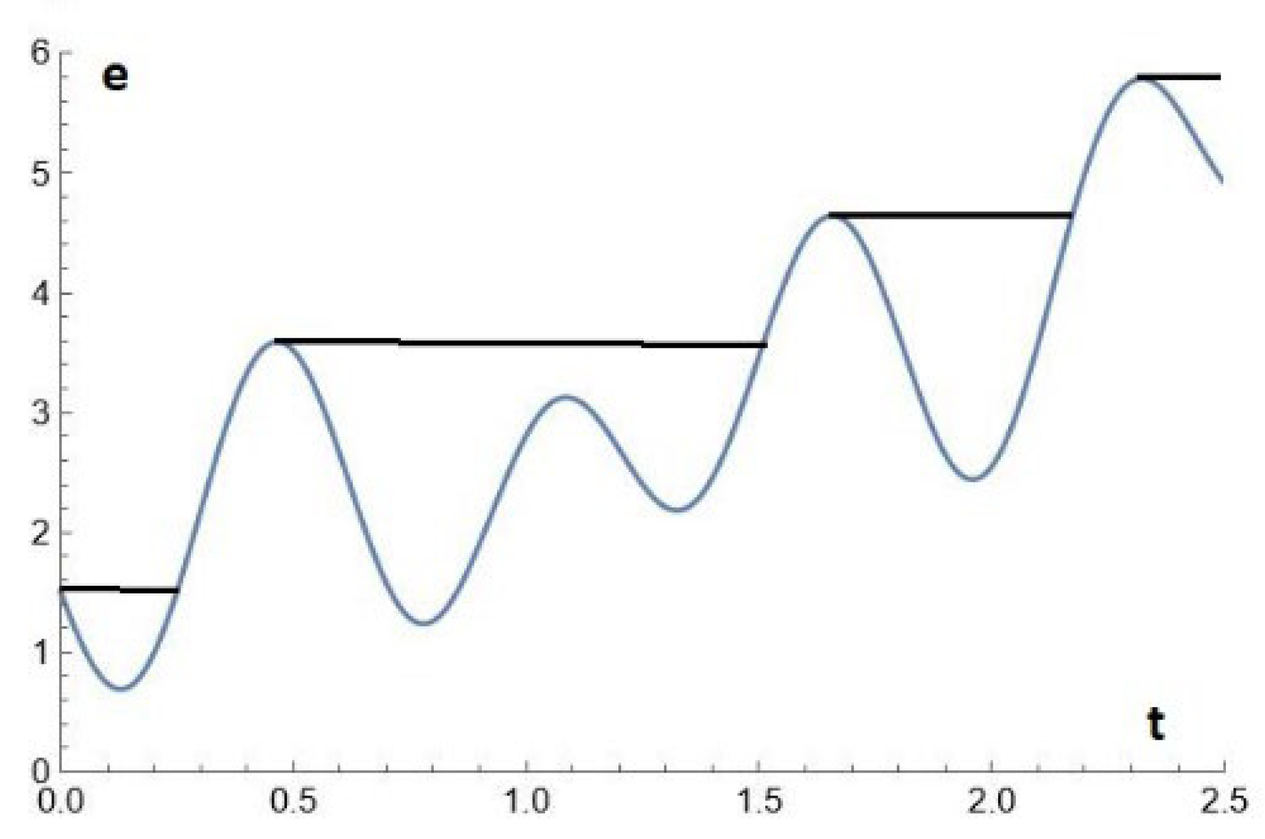
Instead of the straight-line e(t) =0.145+εt used above, we can advantageously use other function e(t) of the proposed evolution, such as the one proposed in the other allegorical figure below (which is a regular curve with relative maxima and minima, Figure 4). The time will appear very slow, so that we can consider the state of the system as a sequence of asymptotic states on the attractor (in the particular case where the attractors are points, we say it's a quasi-static evolution). By taking a larger b, the onset of cycles is delayed.
Figure 4.
Another function e(t) of the proposed evolution, a regular curve with relative maxima and minima.
Figure 4.
Another function e(t) of the proposed evolution, a regular curve with relative maxima and minima.
5. Miscellaneous Examples with Variation of One or More Significant Parameters.
Numerical example -5a- :
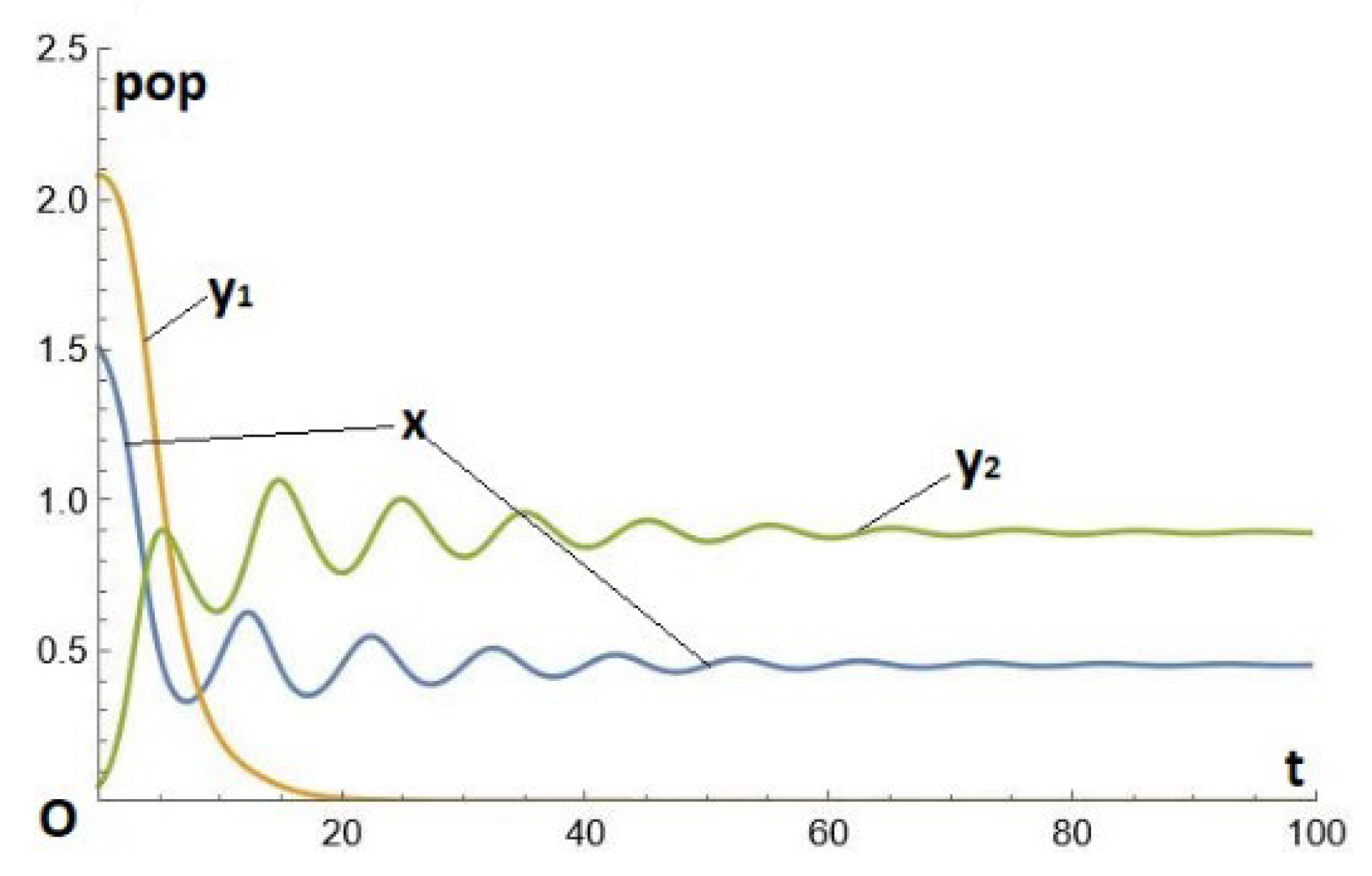
We take advantage of the well-known property that increasing b delays the bifurcation of PAH to modify the numerical example -2- with a much higher b. We then set the e2 value even higher, and the paradox becomes even more obvious. We start from the equilibrium of x with the y1 and the choice of evolution is based on the equilibrium of x with the y2, which involves demographic losses of prey from 1.51 to 0.45 and of predators from 2.08 to 0.9. This situation is close to the "killing of the goose that lays the golden egg". Specifically, the parameters are given by Eq. (18) below, See Figure 5(a).
Figure 5.(a).
Temporal series for system (1)-(2)-(3), where the parameters are given by Eq. (17bis).
Figure 5.(a).
Temporal series for system (1)-(2)-(3), where the parameters are given by Eq. (17bis).
Numerical example -5b- :
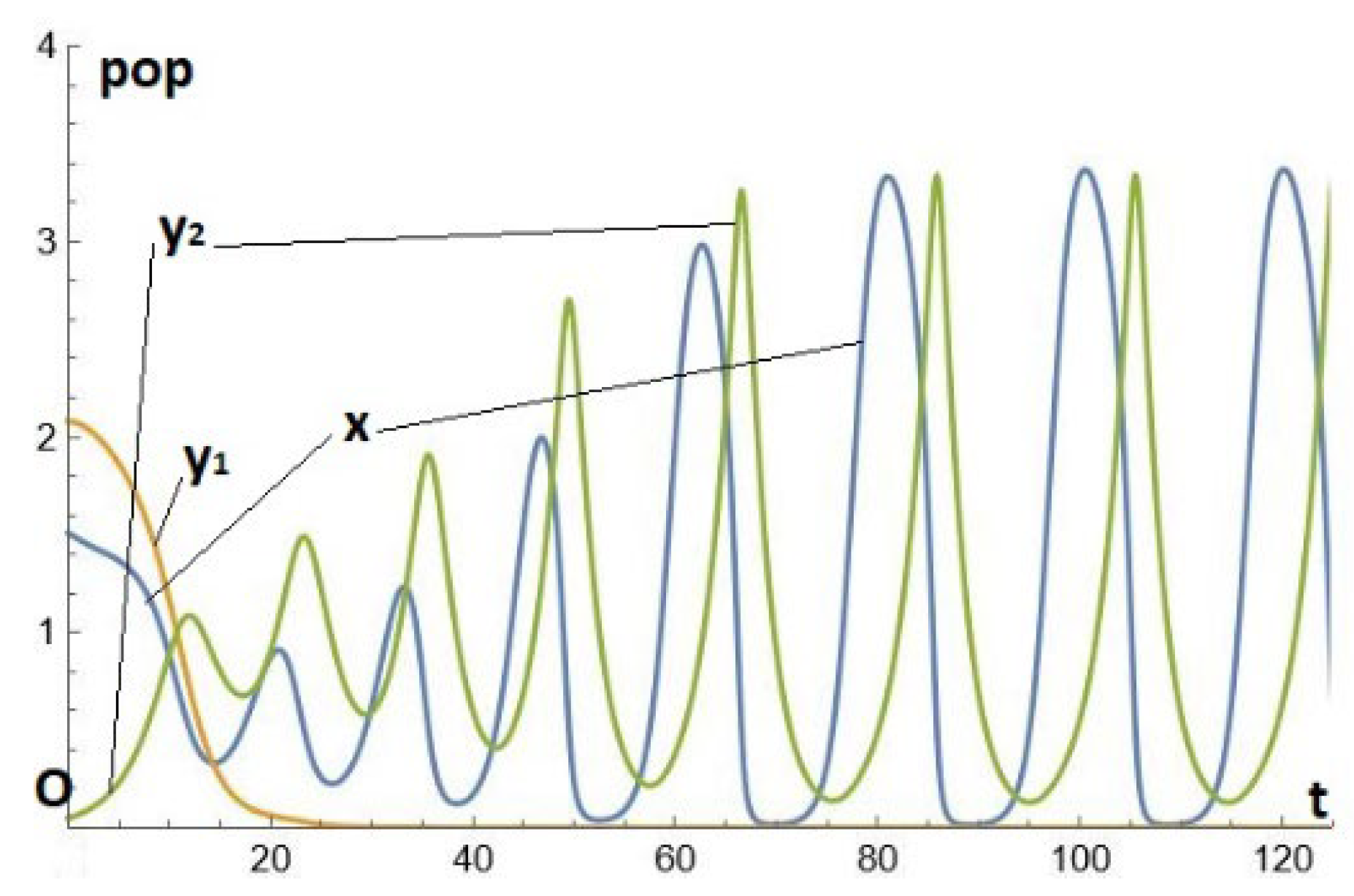
Figure 5(b) below, is close to the previous one, but with a much smaller b2 (b2 =0.8), keeping b1=3. This is a first example of evolution by changing e (to a large value) and b (to a smaller value). Both e and b tend to increase, and e prevails. The result is a replacement as in the previous example, but the final result is oscillating, which could be described as a kind of "intermittent paradox". Specifically, the parameters are given by Eq. (18), but with ; see Figure 5(b).
Figure 5.(b).
Temporal series x(t), y1(t) and y2(t) for system (1)-(2)-(3), where the parameters are given by Eq. (18), except for .
Figure 5.(b).
Temporal series x(t), y1(t) and y2(t) for system (1)-(2)-(3), where the parameters are given by Eq. (18), except for .
Numerical example -5c- :
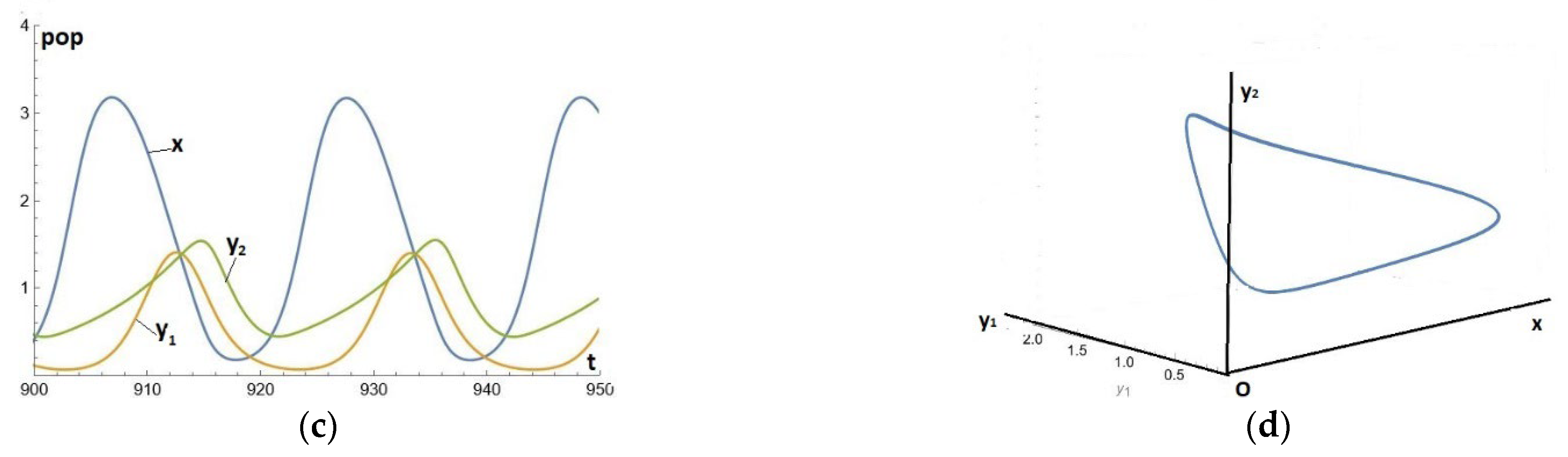
In the previous example, it is sufficient to reduce a little further the value of (from 0.8 to 0.55) to destroy the replacement of by Instead of this, the two predators cohabit (in addition to the prey) in an internal stable cycle. This is an example of the persistence of two predators on a prey, see [5,12,13,14] or [1] chap 10 on this interesting subject. Naturally, this type of solution cannot exist in the cycle-free region (i.e. with e small enough to be below the PAH bifurcation). See Figure 5(c)-(d).
Figure 5.(c-d).
Solutions for system (1)-(2)-(3), where the parameters are given by Eq. (18), except for .(c) Temporal series (t,x), (t,y1), (t,y2) (d) The limit cycle in the (x,y1,y2)-space.
Figure 5.(c-d).
Solutions for system (1)-(2)-(3), where the parameters are given by Eq. (18), except for .(c) Temporal series (t,x), (t,y1), (t,y2) (d) The limit cycle in the (x,y1,y2)-space.
6. Predation-Commensalism System and the Role of Neutral Parameters.
It will prove useful to present here a slightly more complex system, which was introduced in [1] chap 9) to model the global economy. Precisely the interpretation in terms of this system of the well-known property of TRPF (Tendency of Rate of Profit to Fall), which concerns the parameter c, was the starting point of the present work.
In this system, known as predation-commensalism, predation activity exerts a beneficial function on the prey substrate, increasing the capacity of the environment. In concrete terms, the predation-commensalism system is still (1)-(2)-(3), but the capacity of the medium P is no longer a constant, but a function of x:
where the new (positive) constants and are the capacity of the substrate in the absence of predation activity and the coefficient of influence of this activity on capacity. is completely independent of the predator, whereas depends on it in its relationship with the prey, so that in the case of two competing predators, the system is naturally (7) with
This system is always of the form (9) so the properties of section 3 remain valid. It is remarkable that the parameters and , which, as we have just indicated, are clearly associated with one or other of the predators, are nevertheless perfectly neutral in the evolutionary competition. From a mathematical point of view, this follows from equation (11), which does not contain them. From a modeling point of view, this property is perfectly natural, since the influence (coming from either of the two predators) is put into the common pot (capacity of the environment in terms of prey quantity) and therefore constitutes no advantage or disadvantage for one of the predators over the other. In particular, if the two predators differ only in the values of , the system has the first integral y2/y1 =constant as it follows from (11) with q1=q2.
On the other hand, commensal terms have a huge influence on the equilibrium population of predators. We also observe that the value of the x0 of the equilibrium is independent of these new terms; it therefore appears that the terms of influence of predation on the substrate capacity are reflected on y0 and not on x0. This (still paradoxical) property is a consequence of the property reported at the end of section 1 that x0 is obtained directly from the equation in y', which is not concerned by .
It is therefore clear that the parameters e,τ,b and c retain the properties reported in Section 4 with regard to their character as advantages or disadvantages in the competition, while is neutral. A consequence of this is that parameter , while being elusive by the competition when it is the only one to undergo a variation, can be dragged along by even an infinitesimal variation of e, c, b, τ. It is therefore highly unstable.
Numerical example -6a-:
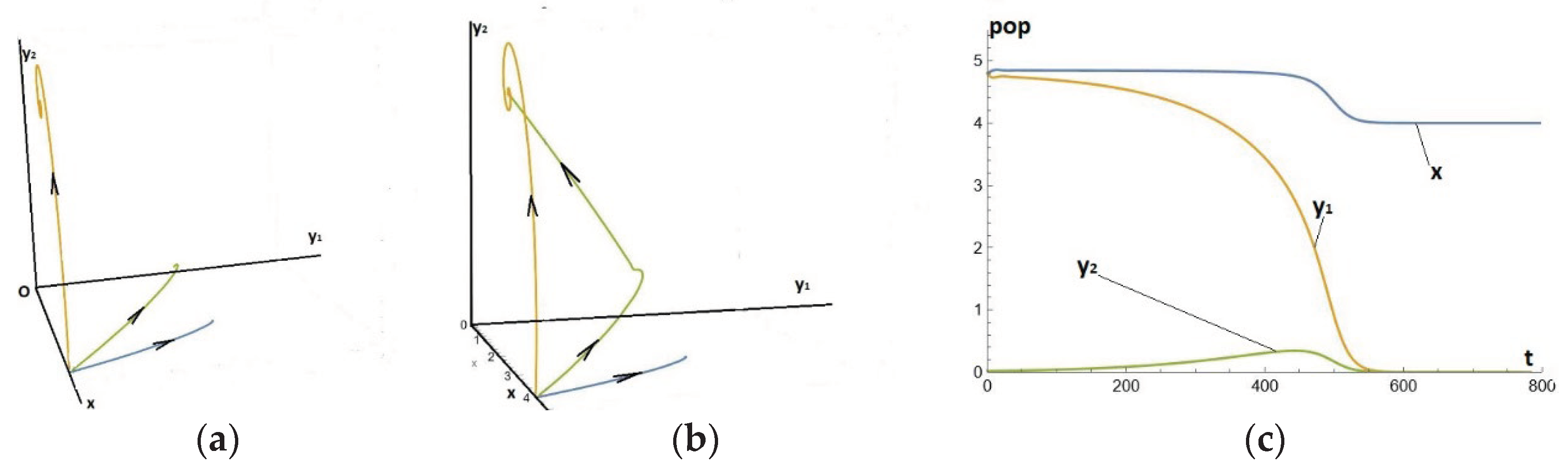
We start with an example in the non-paradoxical region, with values of all parameters equal for both predators, and add commensalism terms . Figure 6(a) shows three orbits in space starting from points close to the equilibrium of the prey alone. Starting with (resp ) we naturally have an orbit for the system of (resp ) alone; the orbits are naturally in the coordinate planes. This clearly shows the demographic advantage of compared with . But starting with non-null and , the orbit is in the plane and in no way chooses at the expense of See Figure 6(a) in which the parameter values are given by Eq. (21),
a=1.0, = 4.0, b1 = b2 =1.0, e1 =e2 =0.18, c1=c2=0.45, τ1=τ2 =1.0, λ1 =0.25, λ2 =1.25
Numerical example -6b-:
We repeat exactly the previous calculations (example -6a-), with parameter values as given in Eq. (21), but taking (instead of 0.45). This minimal difference implies that evolution chooses, and disappears (Figure 6(b)). It can also be seen that the three-dimensional orbit clearly has an initial phase very little different from that of the previous case (fast dynamics), followed by a second phase where it joins the attractor on the plane (slow dynamics).
Numerical example -6c-:
This is now an analogous case with loss of instead of gain. More precisely, we choose a system in x,y2 with λ2 = 0, and e2=0.101, sufficiently small for predation not to be viable, so that the attractor is simply the equilibrium of prey alone The system in has even smaller efficiency but, thanks to the commensalism term (with ), there is a stable equilibrium with Competition between the two populations naturally chooses who has greater efficiency, and so it disappears. Figure6(c) shows this process starting from a point very close to the system attractor in The two predators disappear. The parameter values are given by Eq. (21) but taking e2 =0.102 and λ1 = 2.2, λ2 = 0.
Figure 6.
Predation-commensalism system (1)-(2)-(3), with a capacity of the medium P as a function of x given by Eq. (19). In the case of two competing predators, the system is Eq. (7) with Eq. (20). The parameter values are given by Eq. (21): (a): shows three orbits in space starting from points close to the equilibrium of the prey alonewith ; the third orbit starts from (4, 0.04, 0.02). (b): with (instead of 0.45). (c): with λ1 = 2.2, λ2 = 0 and e2=0.101 (instead of λ1 =0.25, λ2 =1.25 and e2 =0.18).
Figure 6.
Predation-commensalism system (1)-(2)-(3), with a capacity of the medium P as a function of x given by Eq. (19). In the case of two competing predators, the system is Eq. (7) with Eq. (20). The parameter values are given by Eq. (21): (a): shows three orbits in space starting from points close to the equilibrium of the prey alonewith ; the third orbit starts from (4, 0.04, 0.02). (b): with (instead of 0.45). (c): with λ1 = 2.2, λ2 = 0 and e2=0.101 (instead of λ1 =0.25, λ2 =1.25 and e2 =0.18).
7. Conclusion and Discussions
Within the general framework of mathematical ecosystems ecology, the aim of this work is to show how, in a number of situations that are perfectly plausible from an ecological point of view, the choice of evolution is not based on the demographic advantages of the populations in question, but on the functional refinement of the mechanisms (particularly predation) that link them, leading to the appearance of new structures, particularly of a pulsating nature. These are functional emergence phenomena, sometimes to the detriment of the quantitative properties of populations.
An important point is the consideration of the significant parameters of the functional mechanism under consideration, whose variations are proposed at the choice of the evolution, unlike the mathematical theory of structural stability, which involves general disturbances.
The starting point is an analogy with the general law of Tendency of Rate of Profit to Fall (TRPF) in the global economy. This law, initially derived from heuristic considerations, can be obtained mathematically from appropriate models of the economy (see [1] chap 9 sect 9.3). The epistemological status of the properties we are establishing is analogous to those of the TRPF. It's a kind of general tendency, a vocation that occurs under specific conditions (and often in the absence of others), but not automatically.
We have focused on the role of parameter e (the efficiency of the predation mechanism), whose role it is useful to understand. Under conditions of scarcity of prey population x, it is the ratio of the number of preys consumed per unit of predator and time, and the prey population. This is the pure predation mechanism, with no relation to the predator's needs and abilities (which relate to other parameters). Clearly, e depends not only on the physiological properties of prey and predator, but also on environment and habitat, and can be easily influenced by environmental agents. This is why it seems obvious to us that the parameter e is subject to disturbance under conditions where all the others (particularly physiological ones) remain constant.
However, the parameter e of predation efficiency enjoys paradoxical properties with regard to equilibrium populations and their stability. For moderate values of e, an increase in its value leads to an increase in the equilibrium population of predators and a decrease in that of preys (which seems normal), but beyond a certain value of e, its increase leads to a decrease in both equilibrium populations (of predators and preys alike). This is the paradoxical mode, because the scarcity of preys leads to a lack of resources for predators, whose equilibrium population in turn declines. But, in addition, beyond a certain value of e, the equilibrium loses its stability (Poincaré-Andronov-Hopf bifurcation) and the attractor becomes a periodic cycle around the equilibrium. By further increasing the value of e, the cycle takes on the characteristic shape of a curvilinear triangle; in each period we can distinguish three phases: Hubris (excessive predation, or rapid increase in the predator population to the detriment of the prey population), Nemesis (punishment for hubris, or subsequent reduction in the predator population) and Resilience (or slow recovery of the preys, back to the initial state). Finally, for very high values of e, the periodic phenomenon takes on a form akin to that of seasonal epidemics (the predator population is always practically zero, except at certain moments periodically spaced in time).
Our work shows why and how, when two predators compete for prey, evolution always chooses the most efficient predator (and not any kind of population optimization).
As a result, the efficiency e of the predation mechanism appears to be an emergent property, which can only increase through evolutionary choice when the suitable conditions are present, and is therefore irreversible in this context. This implies a natural tendency for periodic cycles to emerge, and even for them to be structured into sequences of hubris, nemesis and resilience. This tendency often runs counter to demographic optimization.
Furthermore, since the choice of evolution is also based on increasing e, as the period increases according to evolution, it sweeps through a wide range of frequencies, making it possible synchronization with other phenomena through small interactions. This furnishes a plausible explanation to the fact that seasonal phenomena are very widespread. Indeed, synchronization is a ubiquitous phenomenon characteristic of many processes in natural systems and (nonlinear) science. It is today considered as one of the basic nonlinear phenomena studied in mathematics, physics, engineering or life science, see for example [1] chap 12 or [15] and references therein cited.
Obviously, the phenomena become much more complex if variations in several significant parameters are simultaneously involved. Several examples have been given (sections 5 and 6), in particular one that leads to a non-choice (example of the coexistence of two predators, often controversial).
It's worth noting, however, that all this is related to the diversity-stability debate, which goes back a long way! See [13,16] or [17]. Indeed, the relationship between diversity and stability has fascinated ecologists for decades. Some argued that more diverse communities enhanced the stability of ecosystems. Others argued that simple communities were more easily disrupted than richer ones, noting that invasions occur most often on cultivated land where human influence has produced highly simplified ecological communities, see [18].
Author Contributions
All authors contributed equally to the interpretation and discussion of results. All authors have read and agreed to the published version of the manuscript.
Funding
This research received no external funding.
Data Availability Statement
Data are contained within the article.
Conflicts of Interest
The authors declare no conflict of interest.
Abbreviations
The following abbreviations are used in this manuscript
| PAH | Poincaré Andronov Hopf bifurcation |
| TRPF | Tendency of Rate of Profit to Fall |
| HNR | Hubris, Nemesis, Resilience |
References
- Sanchez-Palencia, E.; Françoise, J.-P. Dialectique dans les sciences et systèmes dynamiques; Le temps des Cerises, 2022.
- Murray, J.D. Mathematical Biology I: An Introduction; Interdisciplinary Applied Mathematics, 17; Springer-Verlag, New York, 2002.
- Aziz-Alaoui, M.A.; Daher, O.M. Boundedness and global stability for a predator-prey model with modified Leslie-Gower and Holling-type-II schemes. Applied Math. Lets. 2003, 16, 1069–1075. [Google Scholar] [CrossRef]
- Holling, C.S. The functional response of invertebrate predators to prey density. Memoirs of the Entomological Society of Canada 1966, 48, 5–88. [Google Scholar] [CrossRef]
- Lherminier, P.; Sanchez-Plencia, E. On transient processes in attractors in biological evolution, Electronic Journal Diff. Eqt. Conferences 2015, 22, 63–77. [Google Scholar]
- Hassard, B.D.; Kazarinoff, N.D.; Wan, Y-H. Theory and Applications of Hopf Bifurcation; Cambridge University Press, 1981.
- Marsden, J.E.; McCracken, M. The Hopf bifurcation and its applications; Applied Math. Series, 19, New-York, Springer-Verlag, 1976.
- Françoise, J.-P. Oscillations en biologie, Analyse qualitative et modèles mathématiques; Springer, 2005.
- Oli, M.K. Population cycles of small rodents are caused by specialist predators: or are they? Trends Ecol. Evol. 2003, 18, 105–107. [Google Scholar] [CrossRef]
- Basset, A.; et al. Equilibrium concept of phytoplankton communities. In Encyclopedia of ecology, 2nd ed.; 2019; pp. 61–68.
- Hsu, S.B.; Hwang, T.W. Uniqueness of limit cycles for a predator-prey system of Holling and Leslie type. Canadian Appl. Math. Q. 1998, 6, 91–117. [Google Scholar]
- McGehee, R.; Armstrong, R.A. ; Armstrong, R.A. Some mathematical problems concerning the ecological principle of competitive exclusion. Journal Diff. Eqts. 1977, 23, 30–52. [Google Scholar] [CrossRef]
- Sanchez-Palencia, E.; Françoise, J.-P. Topological remarks and new examples of persistence of diversity in biological dynamics. Discrete and Continuous Dynamical Systems Series S 2019, 12, 1775–1789. [Google Scholar] [CrossRef]
- Sanchez-Palencia, E.; Françoise, J.-P. On persistence and invading species in ecological dynamics. Diff. Eqts. and Applications 2021, 13, 297–320. [Google Scholar] [CrossRef]
- Aziz-Alaoui, M.A. Synchronization of chaos. In Encyclopedia of Mathematical Physics; Elsevier, 2006; Volume 5, pp. 213–226.
- McCann, K.S. The diversity - stability debate. Nature 2000, 405, 228–233. [Google Scholar] [CrossRef] [PubMed]
- Sanchez-Palencia, E.; Lherminier, P. Paradoxes of vulnerability to predation in biological dynamics and mediate versus immediate causality. Discrete and Continuous Dynamical Systems 2020, 13, 2195–2209. [Google Scholar] [CrossRef]
- Lewis, M.A.; Petrovskii, S.V.; Potts, J.R. The Mathematics Behind Biological Invasions; Springer International Publishing Switzerland, 2016.
Disclaimer/Publisher’s Note: The statements, opinions and data contained in all publications are solely those of the individual author(s) and contributor(s) and not of MDPI and/or the editor(s). MDPI and/or the editor(s) disclaim responsibility for any injury to people or property resulting from any ideas, methods, instructions or products referred to in the content. |
© 2024 by the authors. Licensee MDPI, Basel, Switzerland. This article is an open access article distributed under the terms and conditions of the Creative Commons Attribution (CC BY) license (http://creativecommons.org/licenses/by/4.0/).
Copyright: This open access article is published under a Creative Commons CC BY 4.0 license, which permit the free download, distribution, and reuse, provided that the author and preprint are cited in any reuse.


