
Submitted:
06 March 2024
Posted:
07 March 2024
You are already at the latest version
Abstract
Highly diverse agroecosystems are increasingly of interest as the realization of farms' invaluable ecosystem services grows. Simultaneously there has been an increased use of uncrewed aerial systems (UAS) in remote sensing as drones offer a finer spatial resolution and faster revisit rate than traditional satellites. With the combined utility of UAS and the attention on agroecosystems, there exists an opportunity to assess UAS practicality in highly biodiverse settings. In this study, we utilized UAS to collect fine-resolution 10-band multispectral imagery of coffee agroecosystems in Puerto Rico. We created land cover maps through a pixel-based supervised classification of each farm and assembled accuracy assessments for each classification. To bolster our understanding of the classifications, we interviewed farmers to understand their thoughts on how these maps may be best used to support their land management. The average overall accuracy (53.9%), though relatively low, was expected for such a diverse landscape with fine-resolution data. After sharing imagery and land cover classifications with farmers, we found that while the prints were often a point of pride or curiosity for farmers, integrating the maps into farm management was perceived as impractical. These findings highlight that while remote sensing of diverse agroecosystems may provide a detailed way of estimating land cover classes and ecosystem services for researchers and government agencies for example these maps may be of limited use to land managers without additional interpretation.
Keywords:
agroecosystem
; drones
; farm management
1. Introduction
Unlike the highly input-dependent monocultures that make up a large portion of the food production system [1,2], diversified agroecosystems are increasingly touted as invaluable systems against climate change. Agroecosystems, in the context of this study, have the capacity to maintain ecosystem services, biodiversity, and farmer livelihoods indicating that the highly diverse farms of this paper are part of more sustainable practices [3,4,5]. Coffee agroecosystems are ecologically, economically, and politically significant to the neotropics [6]. Ecologically, coffee is significant because of the species richness it has the potential to promote. While there exists a gradient from which coffee is grown, ranging from unshaded monocultures to shaded polycultures and agroforestry systems, many coffee farms in the neotropics promote biodiversity by planting coffee in the shade of overstory vegetation. This overstory vegetation and other cultivated plants intercropped with coffee can provide habitat for wild flora and fauna and regulate ecosystem services necessary for other plant life [7,8,9]. Economically, roughly a third of the world’s coffee production takes place in Latin America [10,11]. Because of the significant economic impact that coffee exports have on the neotropics, government policy has frequently encouraged high-intensity production at the expense of more ecologically sound agroecosystems [12].
Foundational to understanding land change post-climatic disaster is having accurate land cover classifications maps before and after such events. The advent of uncrewed aircrafts (UA), or drones, means that remote sensing imagery can be captured with a much finer spatial resolution, on the order of tens of centimeters [13], than satellites like Sentinel-2A MSI and Landsat 8 OLI, which have resolutions of 10-20 meters and 30 meters per pixel respectively [14]. In addition to the increased spatial resolution, drones do not have defined return times and can be employed whenever desired, and around terrain obstacles. The flexibility and increased spatial resolution of drones mean that UAs have the potential to create vastly more accurate land cover classifications.
While the use of auxiliary data and finer-resolution data may aid in improving classification accuracies, in some cases these classifications only benefit researchers and other outside actors, who hold implicit biases about the land that they are studying [15]. In order to derive practical tools and analyses from classifications, it is necessary that farmers be included in the mapping and classification of their land. This becomes especially important in such diversified systems, as more nuance can exist in what does and does not constitute a “crop”. In mapping with farmers, researchers also affirm that our work is done in collaboration with the land stewards of what we map [15]. Working in partnership with farmers does lend itself to the potential of misestimating the amount of a certain land cover class in favor of another due to different actors placing significance on certain land cover types. However, to a large extent, this is considered to be outweighed in terms of the benefits of including farmers in the mapping process [15].
This paper was written with the intention of adding more information to the growing literature on the classification of diversified coffee agroecosystems, with an emphasis on the utility of UA and farmer participation in this effort. Our goals were to quantify the accuracy of classifications performed on fine-resolution multispectral data and to explore how speaking with farmers may change the methods or results in which classification occurred initially. It is our hope that should similar research continue, farmer involvement will happen at an earlier stage, and more often so that a better knowledge exchange can occur.
2. Materials and Methods
Our study took place in the coffee-growing mountainous areas of central-Western Puerto Rico. More specifically, farms were surveyed in Utuado, Adjuntas, Jayuya, and Yauco (see Figure 1). Farms in these regions experienced, between 177-229 cm of annual rainfall [16] and are classified as submontane and lower montane wet forests [17]. Soils present in the coffee-growing region include ultisols, inceptisols, and oxisols [18]. Farms surveyed were a part of long-withstanding coffee agroecosystem research in the region and spanned across a gradient of coffee production intensification [8]. Other commonly found crops in these diverse agroecosystems include citrus trees, bananas, and plantains. The farms surveyed had an average slope of 15.4 degrees. Farms ranged from 0.8-56.7 hectares in size. More information can be found in Table 1.
The uncrewed aircraft (UA) flights used in this study were conducted in 2022to collect 10-band multispectral imagery. Before 2021, numerous preliminary data-gathering missions occurred with the use of fixed-wing and multirotor UA. Ground data collection, which includes the GPS and plant characteristic data, occurred in 2021, 2022, and 2023. Interviews with farmers were conducted in May of 2023 and were subject to review and exemption approval by the Institutional Review Board (IRB) of the University of Michigan.
2.1. Ground Data Collection
Ground data collection was conducted in field campaigns in 2021, 2022, and 2023 to create control points to train and test land cover classification accuracy. We used the ESRI Collector or ESRI Field Maps smartphone app to capture data from a linked external GNSS receiver. In earlier campaigns, the Trimble R1 was used, and in later campaigns, a BadElf Flex was used. Both of these external GNSS receivers were placed on a 2-meter tall survey pole in order to assist in an appropriate satellite connection. Both external receivers increased GPS accuracy (as compared to integrated GPS in the smartphones used to capture data), but steep topography meant that strong connections to satellites were not always met, resulting in decreased GPS accuracy. The Trimble R1 Receiver typically receives submeter accuracy [19], whereas the Bad Elf Flex receives 30-60cm accuracy on average [20]. Because of the steep topography, typically accuracies of below 1 meter were accepted. On very few occasions, accuracies were accepted at around 1.5 meters if a given surveyor had waited five minutes with no increase in accuracy.
At a given crop or plant of interest, the survey pole with attached external GPS was placed as close to the base of the plant as possible. Using a smartphone and either ESRI’s Field Maps or Collector, a GPS point was recorded. The data capture software recorded various information for each GPS point. If the plant of interest was coffee, information on the coffee leaf rust (CLR) and leaf miner level was recorded. Other information collected included the plant type, specific plant species if relevant, farm code, percent of plant covered by vines, notes about the surrounding canopy, date and time of point collection, and a photo of the plant or surroundings if desired.
2.2. Remote Sensing Flights with Uncrewed Aircraft
The uncrewed aircraft (UA) flights used in this study were conducted in 2022 to collect 10-band multispectral imagery. UAS work and subsequent methods documentation were in accordance with Federal Aviation Administration’s (FAA) 14 CFR Part 107 regulations. Highly variable topography within the coffee-growing region of Puerto Rico required significant mission and flight planning in order to collect quality multispectral and LiDAR data. Mission planning was completed prior to arrival in Puerto Rico, and included tasks such as identifying appropriate equipment and sensors for the specific terrain and creating standardized procedures. Google Earth Pro was first utilized to identify farm boundaries and areas within farms that may be of special interest, in addition to being used to identify potential divisions for farms that were too large to be imaged with a single drone flight.
A DJI Inspire 2 multirotor UA was outfitted with a multispectral imaging sensor. Multispectral imaging for relevant field campaigns was done using a MicaSense RedEdge-MX Dual Camera Imaging System, which included 10 synchronized bands that spectrally overlapped with Sentinel-2A MSI and Landsat 8 OLI imagery (detailed in Table 2).
On site, a waypoint-defined flight plan was created in DJI Ground Station Pro on a mobile tablet. The size of the farm, data needs, and underlying surface were considered in determining whether a single or double grid (cross-hatch) flight pattern was flown (Figure 2).
Prior to farm classifications, basic image processing was done in Agisoft Metashape in order to create a georeferenced orthomosaic [21]. The default processing was done utilizing the GPS data generated by the UAS and MicaSense dual camera data capturing process, with no additional manual ground control point input. Reflectance calibration was performed, but no reflectance normalization was performed across flights or farms.
2.3. Image Processing and Classification
The 2022 images were pre-processed and classified for interviews with farmers in 2023. In order to run comprehensive, farm-level classifications, it was determined that for farms that had multiple multispectral images (UA flights), the various images should be mosaiced to create one image per farm. Mosaics were done in ERDAS IMAGINE using the MosaicPro tool, with an “overlay” overlap function specified, default “optimal seamline” generation option was chosen and color corrections were set to “histogram matching”.
Pixel-based supervised classifications were run in ArcGIS Pro 3.1. After loading in the mosaicked farm image, the ground control points (GCPs) from three field campaigns were also layered on top. A classification schema was created to encompass the dominant crops and land cover types across the farms, based on previous visits. This schema included the following ten classes: coffee, citrus, banana, palms, low herbaceous vegetation/grass, bare earth, pavement, buildings, water, and overstory vegetation. For each class, training site polygons were drawn using GCPs as a reference. For instance, if creating a training site for coffee, a polygon was drawn around whichever coffee plant(s) a GCP identified as coffee. For farms that may be larger, significant areas of land would have no GCPs. In order to create representative training sites across the entirety of a farm, polygons were drawn in areas without GCPs that were visually confirmed to match plants with associated GCPs. After creating ample training sites for each class within each farm, a support vector machine (SVM) classifier was run on the entirety of the farm. As we expected that many farms would have limited training classes for a given class, we selected SVM because classifiers make no assumptions about the data distribution [22] and is less susceptible to an imbalance in training samples [23].
After preliminary classifications were completed, interviews occurred, and analysis was finalized after the interviews. Accuracy assessments were run using testing created with the same process as the training sites. For each farm, roughly the same number of testing sites and training sites (0-15 sites depending on the farm and class) were created for a given class. As much as possible, testing sites did not overlap with previously created training sites, with a few exceptions. For instance, farms with water bodies typically only had one small pond. Testing sites were used as reference data for the accuracy assessments, which were then run. We tested additional iterations of classifications utilizing principal component analyses (PCAs) to determine if accuracy was increased by the addition of more data (Table 3).
2.4. Farmer Interviews
In May 2023, we conducted semi-structured interviews with farmers, land managers, and owners, with references made to the multispectral imagery and the classifications. For this purpose, we made posters of each farm’s multispectral imagery and classifications in ArcGIS Pro 3.1. These posters were then printed on 32” x 40” matte paper These interviews were done with the intention of better understanding land use history, farmers’ spatial relationships with their farms, and how remote sensing or land cover classifications may improve the management or understanding of such complex agroecosystems. Interviews were conducted onsite at farms, or at homes on farm property with teams of 2-3 researchers. Interviewees were asked if they consented to both the interview itself, as well as being recorded during the interview using an audio recorder. See Appendix A for more information on the interview script.
Our interviews assumed that we would be referencing the printed orthomosaics and classifications, but many interviews also included walking areas of the farm with farmers as they pointed out specific crops or landmarks. Interview length varied greatly, with some interviews under an hour and others over two and a half hours. This length variation is primarily because interviews were farmer guided, with respondents addressing topics they felt relevant. After a series of questions that were intended to orient researchers to the specifics of a given farm, the multispectral image was shown to the farmers. This was intended to show the farmers what the UA had collected, as well as compile any preliminary thoughts the farmers had on the UA itself. In earlier interviews, tracing paper was laid on top of the multispectral image and farmers were encouraged to annotate any areas they felt important or of general interest. Annotating tracing paper was later removed as part of the interview process, as farmers were often more comfortable speaking generally about the land. After viewing the multispectral image, the classification image was brought out, and farmers were asked questions about the utility of the classification in their management. Viewing the classification map was largely considered to be the conclusion of the interview, and farmers were asked if they had any questions for the researchers. Both the multispectral imagery and the classification maps were left with interviewees at the conclusion of the discussions.
After the interviews were completed, they were uploaded into transcription software and transcribed in Spanish. Researchers then translated the transcriptions from Spanish to English, making corrections to the transcriptions where the software failed to capture any regional language differences or language not otherwise captured. A content analysis was run on the interviews, which included coding each interview transcript individually, as well as synthesizing notes from interviews that were not recorded. In order to conduct an effective content analysis, each theme was clearly defined by researchers. Examples or quotes from interviews were highlighted and sorted into relevant themes. Each example was again reviewed by researchers to ensure that a given example fit into the theme it was assigned to. Each theme was linked to a more generalized research finding from the interviews, and the relevancy of each theme to the project at large was defined. Results were then summarized and put into a content matrix.
3. Results
3.1. Ground Data and Image Capturing
The results of drone flights for 2022 were largely successful. 10 farms were surveyed with both LiDAR and multispectral imagery. Table 4 details the number of flights flown per farm. Of these 10 farms, all but two (ADJUCP and ADJU7) were classified. ADJUCP was not classified as we were unsure if an interview would occur with land managers, and ADJU7 was not classified as large amounts of water were highly reflective and changed the color balance of the farm mosaic.
The results of the ground data field campaigns are listed in Table 5. In 2021, time constraints meant that ground control points were not able to be taken in UTUA16. In 2023, GPS errors on farms UTUA30 and ADJU8 were unable to be resolved in a timely manner, therefore little to no GPS ground truths were collected. Additionally in 2023, no points were collected in YAUC4 due to a thunderstorm that made it unsafe for researchers to conduct ground research. The most points taken occurred in farm JAYU2_3 in 2021. UTUA2 had the most points taken throughout the field campaigns, seemingly because of its proximity to researcher housing.
3.2. Classifications and Accuracy Assessments
An example classification result is shown in Figure 3. Classification figures for all other farms can be found in Appendix B, Figure A1, Figure A2, Figure A3, Figure A4, Figure A5, Figure A6 and Figure A7. Training and testing sites are detailed in Table A1, Table A2, Table A3 and Table A4 in Appendix C. Both training and testing sites are quantified in two forms: polygons and pixels. Polygons designate the number of sites drawn, and pixels refer to the total number of pixels across all polygons.
The initial landcover classifications were all assessed for accuracy. Table 6 details both the overall accuracy of the classification, as well as the Cohen’s Kappa statistic. The Cohen’s Kappa statistic incorporates errors of commission and omission and is regarded as more nuanced than that of overall accuracy [24]. Kappa is reported on a scale of -1 to +1, with values closer to +1 indicating a stronger classifier. A classifier is considered strong if it has a high accuracy while considering the expected accuracy of a random classifier [25].
The average overall accuracy across all farms was 53.9% and the average Kappa statistic across all farms was 0.409. Farm YAUC4 had the highest overall accuracy, as well as the highest Kappa statistic. The lowest accuracy and Kappa statistic for classification was farm UTUA16. Individual accuracy assessments, including users’ and producers’ error, can be found in the Supplementary Material, Tables S1–S9.
Our secondary classification results were similar to those of the initial classification, but ultimately did not improve classification accuracy consistently. Because of this, they were omitted from the paper but more information on their results can be found in Appendix D, Table A5. Individual accuracy assessments for secondary classifications can be found in the Supplementary Material, Tables S10–S19.
3.3. Farmer Interview Content Analysis
We conducted a total of nine interviews, six of which were recorded on an audio recorder, following the interviewee’s consent. Using the recorded interviews and notes from the interviewees who did not consent to be recorded, we created a content matrix (Table 7) to summarize shared themes across interviews. The themes highlighted included utility, novelty, orientation, biodiversity, clarity, and land management. Farmers found the maps interesting and exciting but were unsure if they were applicable to the land management of their farms. Many farmers struggled to orient themselves, especially when landmarks the farmers were familiar with weren’t overtly visible in the map. Many farmers noted a lack of biodiversity or crops present in the map. Lastly, while viewing maps many farmers noted current or future management decisions they consider. These were included in the content matrix as they may inform future iterations or methodologies of classifications.
4. Discussion
We learned from our interviews with farmers how our maps could be improved in terms of accuracy and relevancy. While diversified coffee agroecosystems have a myriad of potential land cover classes, we initially believed that fewer classifications categories would support the legibility of the maps to farmers who might be unfamiliar with this format. However, many farmers noted that biodiversity and plants that they deemed important were absent from our maps. These exchanges underscore the importance of contextualizing the development of a classification workflow with local knowledge, as it can help identify critical problems that justify extra effort to provide a more relevant deliverable for farmers.
We obtained an average kappa value across all farms of 0.409, meaning that the classifiers, generally, are fair in comparison to a random classifier [26,27]. Many of the farms have a slight disagreement between overall accuracy and the kappa index, for instance YAUC4 had an accuracy of 74% (or 0.74) and a kappa statistic of 0.51. In the case of all classification iterations in this paper, the overstory vegetation class often had more training and testing sites made of larger segments. Even though the overstory vegetation may have skewed overall accuracy, the kappa statistic takes into account the relative impact of each class, meaning that it is not skewed by a single well-represented class [24,25,28], in this case, overstory vegetation. It is worth noting, in this paper and otherwise, that while overall accuracy and the kappa statistic are common ways to evaluate land cover classifications in the remote sensing field, more recent literature [29,30] has highlighted that confusion matrices are not entirely reliable and need to be analyzed with some understanding that the accuracies reported are not absolute.
Somewhat expectedly, many of the vegetation classes (i.e., coffee, citrus, banana, palm, and overstory vegetation) were misclassified as other vegetation classes. Because these classes are spectrally similar, and because the initial classifications utilized all ten bands, including those that have little separation between classes within the same band, it can be anticipated that there would be some confusion amongst these classes. Figure 4 illustrates the spectral similarities across vegetation training classes. Another area of confusion was between the pavement and building classes. Across many of the farms, buildings and pavements were misclassified as one another, but were less often misclassified as bare earth and vegetation.
There exists a myriad of reasons why the land cover classifications of this paper may be considered “inaccurate”, many of which have been alluded to earlier in this discussion. One such reason may be the inability of researchers to distinguish land cover types in multispectral imagery. For instance, on many farms, coffee may be grown under the canopy cover of other vegetation. If all coffee ground control points were obscured by larger overstory vegetation, researchers would be unable to accurately draw training and testing sites. In addition, some classes present on farms, while relevant, lacked sufficient training and testing points due to their rarity. As an example, we trained the classifier to identify citrus in UTUA20, but found that the small number of citrus present meant testing sites were either generated on the same tree training was done on, or testing was unable to be completed.
Our classification results could be improved with additional steps that were not available to us at the time but may benefit future studies. We were unable to conduct radiometric normalization prior to the image mosaicking process, which may have improved consistency across flights and farms [31]. While histogram equalization was conducted during the mosaicking process, the resulting mosaics still had visible radiometric differences. For example, radiometric normalization could have reduced the bright spots present in one flight over ADJU7, which likely led to spectral imbalances that prevented us from successfully classifying the imagery of this farm. In addition, if radiometric normalization occurred earlier in the process, it may have been feasible to train the classifier on only one farm and then apply it across farms. This would reduce the work to create many training sites across farms in order to compensate for the radiometric discrepancies. Additionally, classifications may be improved by using ground control points in orthomosaic creation. During the processing of imagery in Agisoft Metashape, only the internal UA GNSS system was used to georeference raw images. By including ground control points collected with a more precise external GPS receiver in the image processing methodology, multispectral imagery may have been better aligned with ground control points collected for building training sites. More broadly speaking, the inclusion of more GCPs in creating training and testing sites may also improve classification accuracy. However, for some research, the time and labor needed to complete more ground truthing may not be justified by an increased overall accuracy.
Analyzing the interview recordings and notes allowed for a more nuanced understanding of the remote sensing work done in this paper. It became very apparent during interviews that farmers and land managers were extremely excited to view, talk about, and keep the map printouts. Many remarked that the images of their farms were beautiful and were excited to display the printouts for others to see but were unsure of how the maps or products derived from the maps could be implemented in regular management. One farmer noted that they planned to hang imagery in a cafe for visitors to see, but when questioned about the utility of the map in their work, they indicated that they would instead be more interested in utilizing the drone to evenly distribute pesticides.
While the beauty and excitement of images and landcover classification maps are often overlooked as an aspect of utility in the remote sensing field, we understood this to be an extremely important subtheme, as it became more evident that farmers and researchers could build further rapport by addressing the beauty of the images and the farms that land managers work so hard to maintain. Connection building in the context of this paper is extremely relevant as land cover classifications are regarded as an iterative process [15]. By fostering better connections between researchers and farmers, we can more intimately understand the ways in which our work fits into farmers’ management and make adjustments to maps accordingly. In many of our interviews, interviewees often pointed out a lack of diversity or missing landmarks. Without having conversations with land managers, researchers are limited to making changes that may not be useful to farmers and instead only serve to increase classification accuracies for schemas that were flawed themselves.
Farmers who communicated to us that maps were lacking relevant information also had more difficulty orienting themselves during interviews. One farmer remarked that he had often regarded his land as a square parcel and viewing it as the roughly rectangular shape the imagery was captured as led him to become disoriented. The farmer also noted that he might have been able to orient himself in spite of his perception of the parcel, but only if landmarks he passed by daily had been included and labeled as such. When farmers are not able to orient themselves to the imagery, implementation of the maps in management becomes even farther fetched.
While many farmers indicated absent crop and vegetation diversity in the land cover classification map, we felt that sharing a more simplistic map first actually enhanced the feedback we received and farmers’ own understanding of the maps. Because the map shared was simpler, farmers noted specific areas where they were interested in seeing more detail, where they were practicing a given land management technique, or where they had a few personally relevant crops. In addition, we believe that the lack of detail present allowed for quicker orientation and better clarity of understanding of the maps. This was extremely important as we understood that land managers had not ever seen their land displayed in this manner and needed some time to relate the imagery to land they were intimately familiar with.
Including interviews as part of this project greatly enhanced the findings of this paper and would enhance any future work in similar settings. Colloredo-Mansfield et al. found similar results in their work, noting that participatory drone mapping allowed researchers to ascertain broader and more relevant information about land management [32]. In addition, Colloredo-Mansfield et al. found that conducting land cover classification maps allowed them to understand sensitive areas of farms (e.g., where young plants were growing) and establish rapport between researchers and farmers. Following Colloredo-Mansfield et al. [32] it is clear that our project would benefit from more knowledge sharing between researchers and farmers. One farmer noted during our interview that while she was extremely excited about participating in research, she was disappointed that she previously had no proof of the drones being on the property to share with a friend. By leaving her with the printout of the map and a description of the work we had done, the farmer may be more likely to continue working with researchers. In return, we received valuable feedback on the crops and vegetation relevant to her on her property. Similar land cover classification projects would benefit from additional iterations incorporating such feedback and knowledge-sharing.
The detailed nature of the high-resolution imagery was seemingly part of the interest that farmers had in interacting with the printouts. While the pixel-based supervised land cover classifications had fair accuracy, switching to an object-based classification would likely increase the overall average accuracy, as it is documented that object-based classifications perform better, especially at finer resolutions [33]. However, the fine-resolution data presented in this paper comes at a cost of increased processing power and time requirements for each step of image processing and classification. Object-based classifications may require even more computational power, especially at the segmentation step [34].
Classification maps may also be enhanced with the addition of elevation or surface data, like LiDAR data that is collected together with the multispectral imagery, and could be the subject of collaborative data fusion projects. Farmers interviewed also often noted that they oriented themselves using peaks and valleys present on farms, something not reflected in the printout of the multispectral imagery or land cover classification maps. However, including data like this may mandate a more dynamic format in which to present maps to farmers. While digital elevation and surface models are something many in remote sensing are familiar with, viewing elevation data on a 2D plane may still present some challenges for those who have not seen such maps before. This could potentially be remedied by creating a 3D model of the surface or elevation data and viewing it together with farmers on a computer.
5. Conclusions
This study was conducted to better understand pixel-based supervised land cover classifications of diverse agroecosystems, and the utility they serve as management tools. We applied this exploration to coffee agroecosystems in Puerto Rico, contributing to the growing literature on using fine-resolution imagery collected by UAS in remote sensing. We found that while our land cover classifications are only moderately accurate, they have the potential to become more accurate by utilizing different methodologies and better ground truths. In addition, we concluded that while farmers were unsure about using the maps as a farm management tool, they were still excited about the technology being applied to their land. In addition, we found that sharing our maps with farmers, even with their flaws, generated better communication between researchers and farmers and created the opportunity to “be attentive to the ‘social position of the new map and how it engages institutions’ ” [15,35].
However, there still exist many opportunities to expand and improve this research. Improving remote sensing methodologies includes further exploring object-based classifications in the context of Puerto Rican coffee agroecosystems, and improving interviews could include viewing more map iterations in more dynamic forms. Both remote sensing and interview methodologies would be improved by visiting farmers and their land more often. We hope this paper encourages further exploration of fine-resolution remote sensing in coffee agroecosystems. We also hope that this paper encourages more work alongside farmers to create classification schemes and products better suited to the needs of farmers.
Supplementary Materials
The following supporting information can be downloaded at the website of this paper posted on Preprints.org. Table S1–S19: accuracy assessments for all iterations.
Author Contributions
Conceptualization, G.K. and S.B.; methodology, G.K. S.B., and K.A.; software, G.K., S.B., K.A. and R.S.; validation, G.K., N.H., K.L., and R.G.; formal analysis, G.K., S.B., N.H., and I.P.; investigation, G.K., N.H., K.L., R.G., J.C., B.N., and K.A.; resources, S.B., K.A., R.S., and I.P.; data curation, G.K. and S.B.; writing—original draft preparation, G.K.; writing—review and editing, All Authors; visualization, G.K.; supervision, S.B.; project administration, S.B., K.A., and I.P.; funding acquisition, S.B., K.A., and I.P. All authors have read and agreed to the published version of the manuscript.
Funding
This research was funded by USDA | National Institute for Food and Agriculture, grant number 2019-67022-29929.
Data Availability Statement
The data presented in this study are available on request from the corresponding author.
Acknowledgments
We would like to acknowledge the farmers who gave their time and effort to be interviewed. We would also like to acknowledge J.P.D. for his role in troubleshooting and editing.
Conflicts of Interest
The authors declare no conflicts of interest. The funders had no role in the design of the study; in the collection, analyses, or interpretation of data; in the writing of the manuscript; or in the decision to publish the results.
Appendix A
English Version of Interview
Note: The interviews will be conducted in Spanish, but we have included the English version for IRB purposes.
“Hello, my name is Nayethzi Hernandez and this is my colleague Gwen Klenke. We’re both graduate students at the University of Michigan. And this project is in collaboration with Ivette Perfecto, who you know. Thank you for taking the time to participate in this study. As Warren let you know, our team is looking into diverse Puerto Rican coffee farms and agroecology systems. As someone who is so knowledgeable, I really appreciate your time. Through interviews, we’re just looking for generalizable information, and none of this will be identifiable. If that’s still okay with you it’ll take us roughly 1 hour. Before we begin I want to confirm that it’s okay that I record our conversation. Please let me know if anything comes up during the interview you just let me know.
Excellent! Let’s begin talking a bit about your land.
Question group 1: Land history and farm management
Can you tell me a bit about how you started growing coffee?
When it comes to your farm, what are your goals with your crops?
Could you tell me a little bit about how you decided to put which crops where?
What type of knowledge or techniques influence how you manage the farm?
Could you tell me about some of the environmental changes that you’ve experienced while farming this land?
What are some goals you have for your farm?
Question group 2: Show farmers the map
*Translate what Gwen says about how the maps are made*
When you first look over the map what are some of your thoughts?
Question group 3: Map review
After looking over the map, what are areas of the map that are of interest to you?
Are there any changes you would like to consider when looking over this map?
If this technology was available to you would it be helpful for farm management?
If it’s helpful to you, how often would you want an updated map?
Closing:
Thank you so much for your insights! We really appreciate your time. We invite you to keep the map if you’d like it. Before we finish, is there anything you’d like to ask or say to us regarding the map or the interview? I will provide you with my contact information if you have any questions for me about this study, or anything else.”
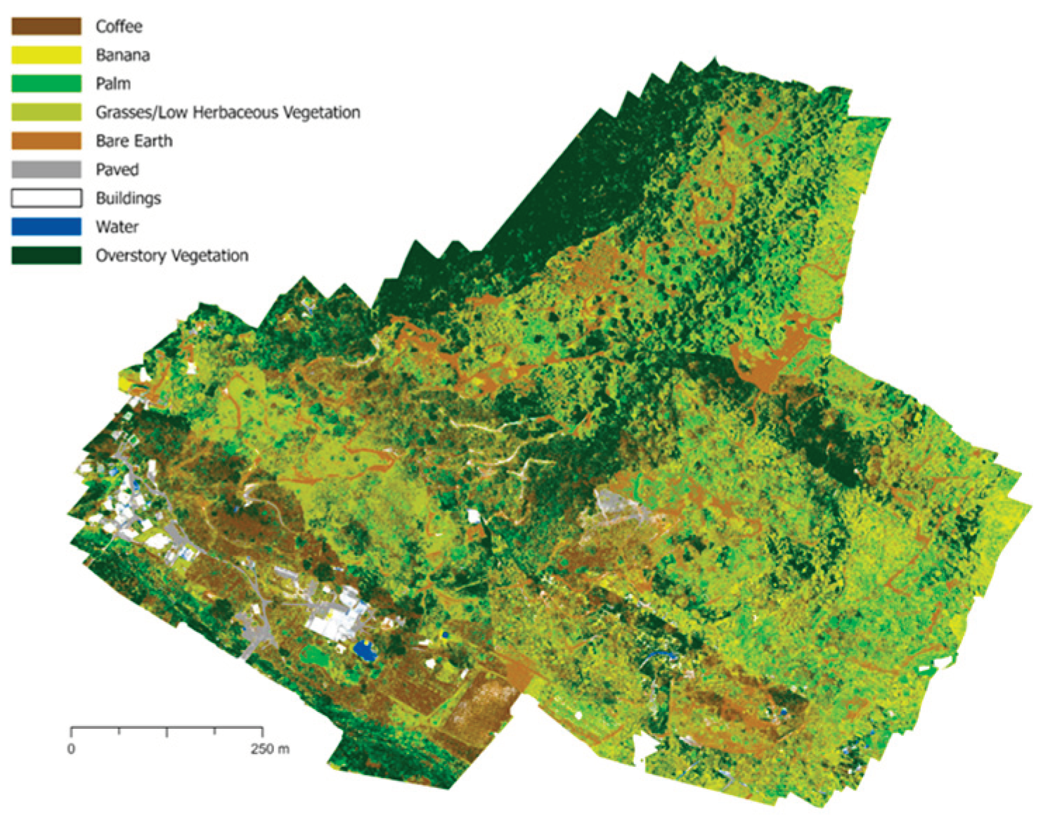
Appendix B
Figure A1.
Land cover classification of farm UTUA16 using 2022 multispectral imagery.
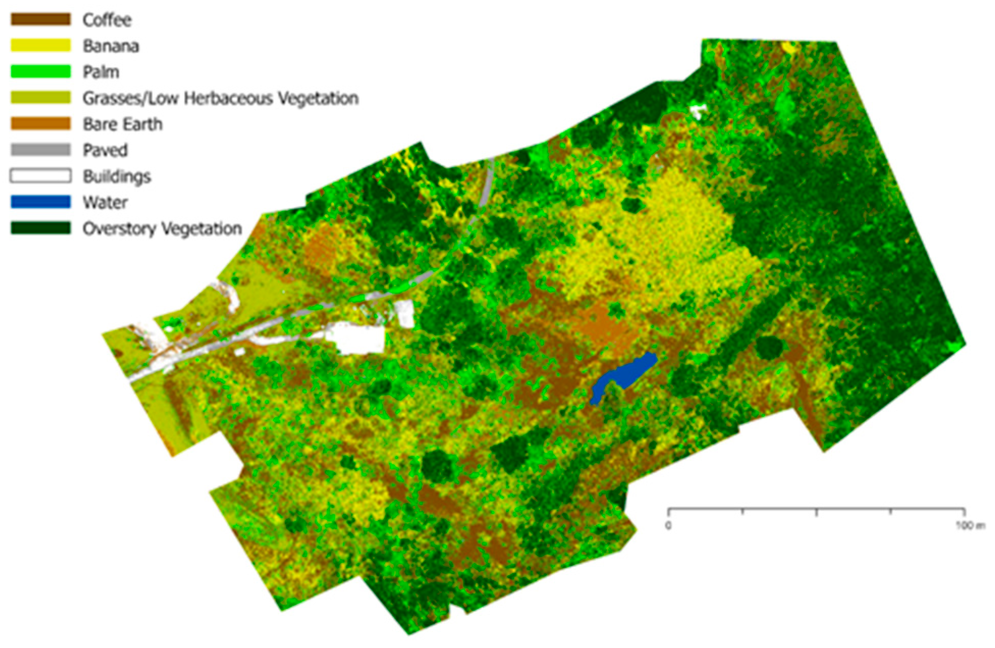
Figure A2.
Land cover classification of farm UTUA18 using 2022 multispectral imagery.
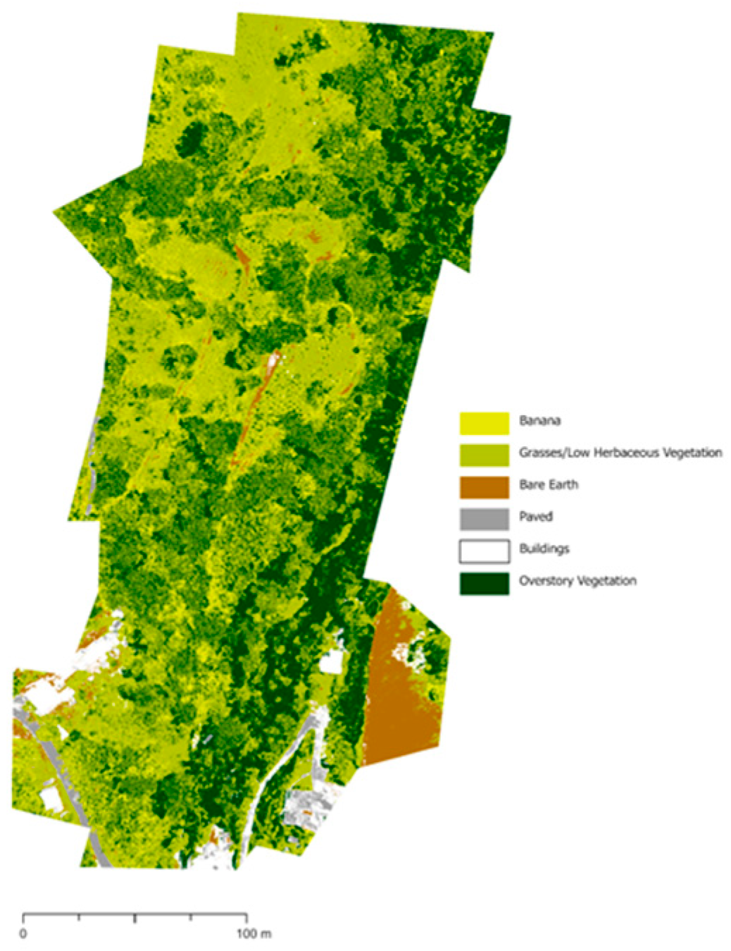
Figure A3.
Land cover classification of farm UTUA20 using 2022 multispectral imagery.
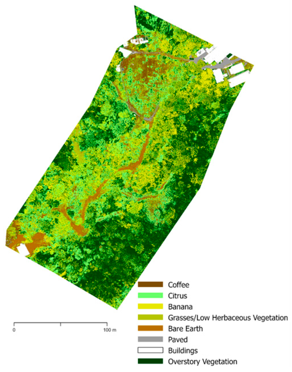
Figure A4.
Land cover classification of farm UTUA30 using 2022 multispectral imagery.
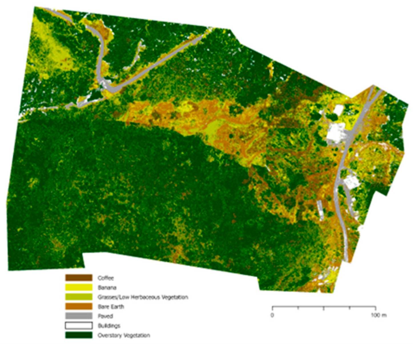
Figure A5.
Land cover classification of farmYAUC4 using 2022 multispectral imagery.
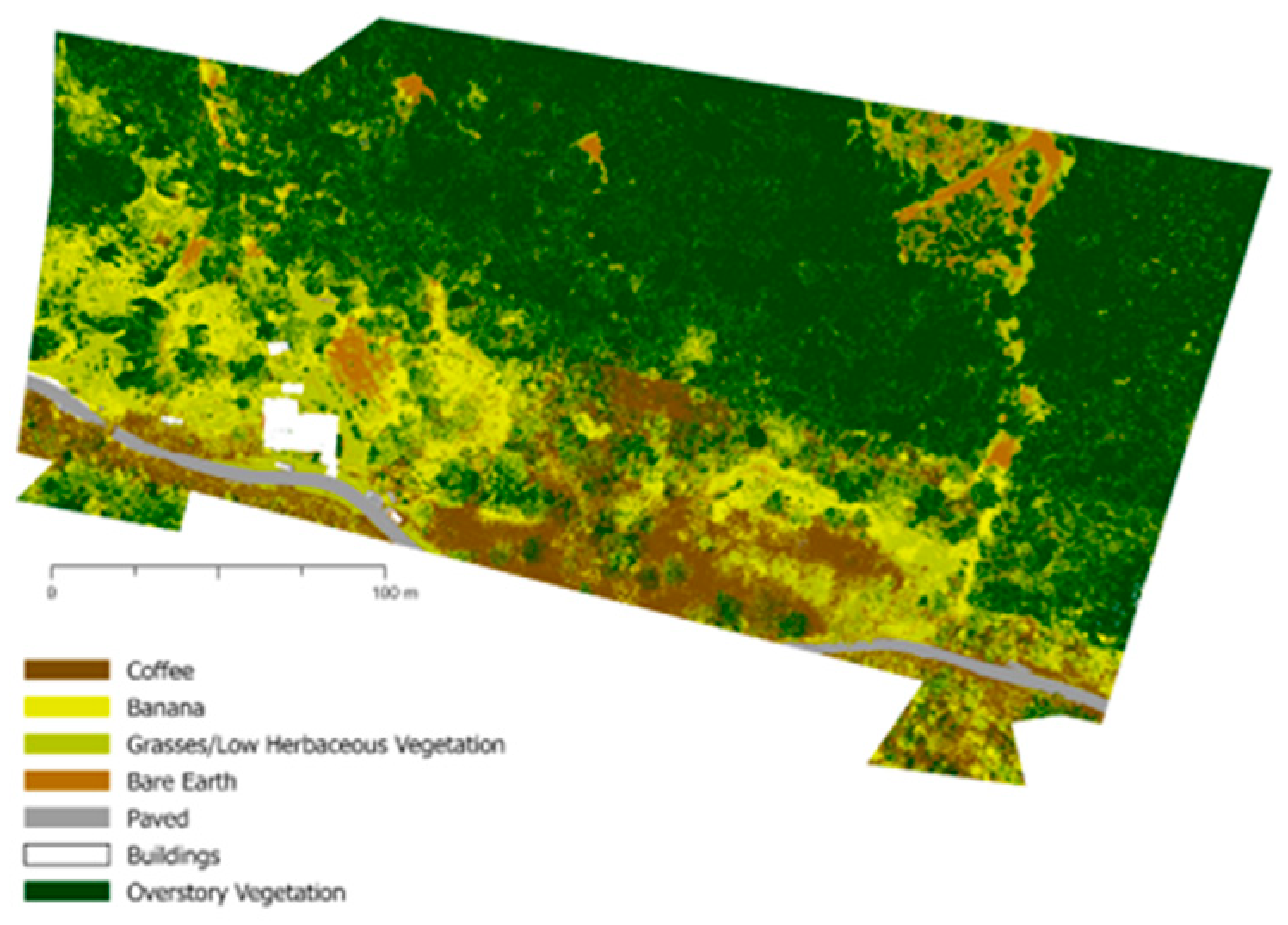
Figure A6.
Land cover classification of farm ADJU8 using 2022 multispectral imagery.
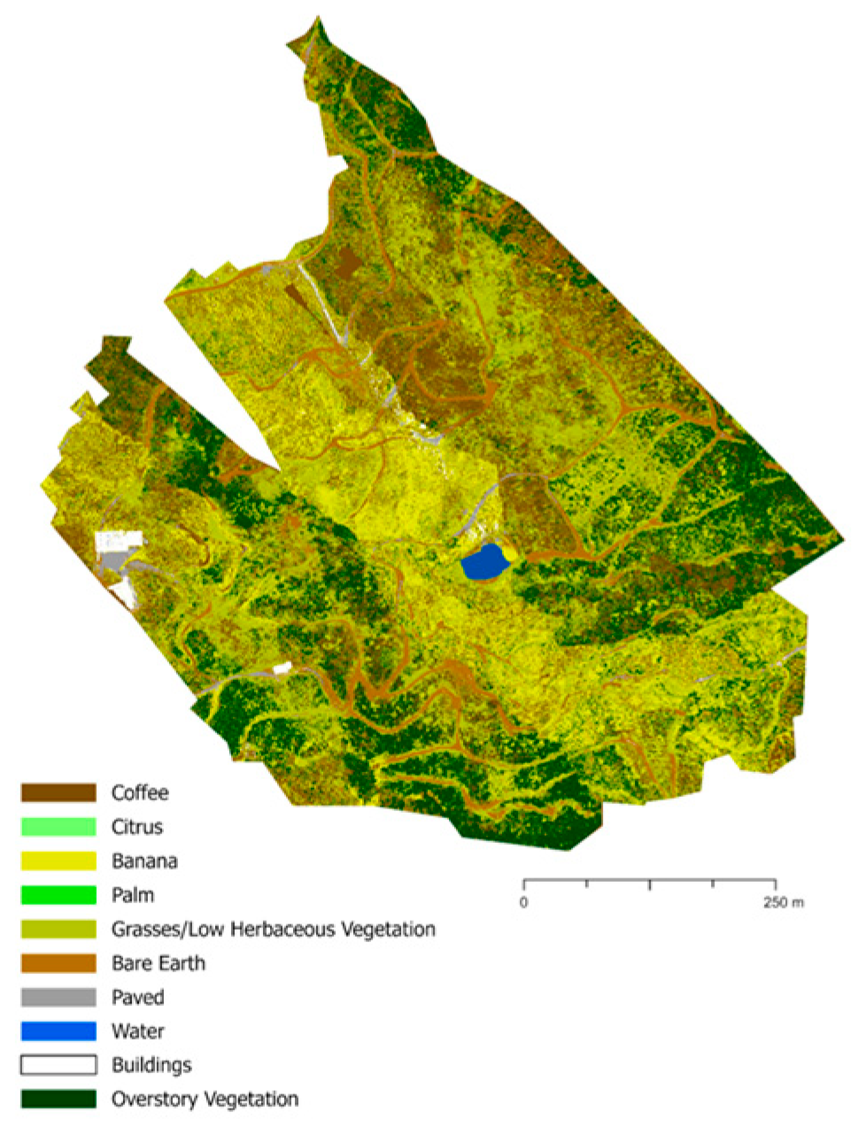
Figure A7.
Land cover classification of farm JAYU2_3 using 2022 multispectral imagery.
Appendix C

Table A1.
Number of training sites for each class in each farm. Each site is a polygon drawn around one representative site.
Table A1.
Number of training sites for each class in each farm. Each site is a polygon drawn around one representative site.
| Farm | sites/polygons | ||||||||||
| coffee | citrus | banana | palm | grasses/low herb | bare earth | paved | buildings | water | overstory veg | total | |
| UTUA2 | 16 | 9 | 3 | 3 | 6 | 6 | 2 | 4 | 0 | 1 | 50 |
| UTUA16 | 3 | 0 | 2 | 5 | 1 | 1 | 1 | 2 | 1 | 2 | 18 |
| UTUA18 | 0 | 0 | 4 | 0 | 3 | 3 | 2 | 2 | 0 | 3 | 17 |
| UTUA18_obj | 6 | 0 | 2 | 0 | 2 | 3 | 3 | 3 | 0 | 2 | 21 |
| UTUA20 | 4 | 7 | 4 | 0 | 2 | 4 | 2 | 3 | 0 | 2 | 28 |
| UTUA30 | 10 | 0 | 8 | 0 | 2 | 4 | 4 | 4 | 0 | 4 | 36 |
| YAUC4 | 9 | 0 | 6 | 0 | 8 | 5 | 4 | 3 | 0 | 3 | 38 |
| ADJU8 | 14 | 0 | 14 | 0 | 10 | 10 | 3 | 6 | 2 | 7 | 66 |
| JAYU2_3 | 22 | 0 | 14 | 11 | 10 | 12 | 7 | 10 | 2 | 11 | 99 |
Table A2.
Number of pixels in training sites per class in each farm classification.
| Farm | pixels | ||||||||||
| coffee | citrus | banana | palm | grasses/low herb | bare earth | paved | buildings | water | overstory veg | total | |
| UTUA2 | 15420 | 89118 | 17989 | 148768 | 60581 | 47051 | 20753 | 185462 | 0 | 130191 | 715333 |
| UTUA16 | 22218 | 0 | 219318 | 164487 | 46675 | 13170 | 4615 | 85679 | 26321 | 448878 | 1031361 |
| UTUA18 | 0 | 0 | 29439 | 0 | 21740 | 113898 | 8102 | 54437 | 0 | 246623 | 474239 |
| UTUA18_obj | 19621 | 0 | 14374 | 0 | 52909 | 161456 | 18481 | 60649 | 0 | 427093 | 754583 |
| UTUA20 | 4467 | 24900 | 218041 | 0 | 28145 | 20922 | 13867 | 176316 | 0 | 346139 | 832797 |
| UTUA30 | 9420 | 0 | 45587 | 0 | 37646 | 18861 | 23754 | 55815 | 0 | 1339405 | 1530488 |
| YAUC4 | 13393 | 0 | 74659 | 0 | 63188 | 49843 | 107538 | 142527 | 0 | 983011 | 1434159 |
| ADJU8 | 36804 | 0 | 10892 | 0 | 96113 | 48835 | 23161 | 99930 | 45674 | 424707 | 786116 |
| JAYU2_3 | 60510 | 0 | 42551 | 47663 | 361668 | 163092 | 57446 | 142129 | 10865 | 635097 | 1521021 |
Table A3.
Number of testing sites per class for each farm. Each site is a polygon drawn around one representative site.
Table A3.
Number of testing sites per class for each farm. Each site is a polygon drawn around one representative site.
| Farm | sites/polygons | ||||||||||
| coffee | citrus | banana | palm | grasses/low herb | bare earth | paved | buildings | water | overstory veg | totals | |
| UTUA2 | 9 | 4 | 4 | 3 | 5 | 5 | 3 | 3 | 0 | 2 | 38 |
| UTUA16 | 0 | 0 | 3 | 3 | 2 | 3 | 2 | 2 | 1 | 2 | 18 |
| UTUA18 | 7 | 1 | 3 | 0 | 4 | 9 | 5 | 5 | 0 | 4 | 38 |
| UTUA18_obj | 7 | 1 | 3 | 0 | 4 | 9 | 5 | 5 | 0 | 4 | 38 |
| UTUA20 | 6 | 0 | 4 | 1 | 3 | 9 | 5 | 5 | 0 | 3 | 36 |
| UTUA30 | 11 | 0 | 4 | 2 | 3 | 3 | 4 | 3 | 0 | 2 | 32 |
| YAUC4 | 11 | 0 | 5 | 3 | 6 | 7 | 3 | 2 | 0 | 3 | 40 |
| ADJU8 | 16 | 0 | 13 | 0 | 10 | 10 | 3 | 3 | 2 | 4 | 61 |
| JAYU2_3 | 22 | 0 | 15 | 4 | 12 | 12 | 7 | 4 | 1 | 5 | 82 |
Table A4.
Number of pixels in testing sites per class for each farm.
| Farm | pixels | ||||||||||
| coffee | citrus | banana | palm | grasses/low herb | bare earth | paved | buildings | water | overstory veg | totals | |
| UTUA2 | 3810 | 17091 | 18297 | 80214 | 54190 | 10729 | 38281 | 125668 | 0 | 203356 | 551636 |
| UTUA16 | 0 | 0 | 7781 | 61145 | 41312 | 9343 | 9845 | 11010 | 37650 | 233632 | 411718 |
| UTUA18 | 2493 | 4121 | 59215 | 0 | 28739 | 22514 | 32468 | 80595 | 0 | 260498 | 490643 |
| UTUA18_obj | 2493 | 4121 | 59215 | 0 | 28739 | 22514 | 32468 | 80595 | 0 | 260498 | 490643 |
| UTUA20 | 2793 | 0 | 21690 | 24840 | 9667 | 23540 | 6096 | 99500 | 0 | 239493 | 427619 |
| UTUA30 | 2483 | 0 | 2546 | 38088 | 35111 | 22465 | 22665 | 31082 | 0 | 137590 | 292030 |
| YAUC4 | 7746 | 0 | 34838 | 79386 | 10584 | 52144 | 24292 | 5484 | 0 | 367339 | 581813 |
| ADJU8 | 18869 | 0 | 43640 | 0 | 49656 | 69418 | 14798 | 51844 | 56798 | 306815 | 611838 |
| JAYU2_3 | 14095 | 0 | 41412 | 28680 | 51561 | 35116 | 33236 | 337495 | 16366 | 296676 | 854637 |
Appendix D
Table A5.
Accuracy of secondary classifications. The table details the overall accuracy of each farm along with Cohen’s Kappa statistic.
Table A5.
Accuracy of secondary classifications. The table details the overall accuracy of each farm along with Cohen’s Kappa statistic.
| Iteration | Farm | Overall Accuracy (%) | Kappa |
| B | UTUA2 | 51.3 | 0.399 |
| UTUA16 | 51.6 | 0.389 | |
| UTUA18 | 55.3 | 0.425 | |
| UTUA20 | 52.7 | 0.395 | |
| C | UTUA2 | 45.4 | 0.361 |
| UTUA16 | 51.2 | 0.376 | |
| UTUA18 | 46.9 | 0.324 | |
| D | UTUA20 | 50.9 | 0.372 |
| E | UTUA2 | 47.3 | 0.380 |
| F | UTUA2 | 45.6 | 0.358 |
Secondary classifications were completed using several alternate band combinations, but overall, the new layer stacks did not lead to an increase in accuracy under these methods. With the exception of three classifications (Iteration B of farm UTUA16, Iteration B of farm UTUA20, and Iteration C of UTUA16), overall accuracies of secondary classifications were lower than the initial classification, although the differences in all cases were only marginal. When considering Iteration A accuracies alongside Iterations B-F, the average overall accuracies cannot be directly compared because not all farms initially classified were used in the secondary classifications. However, when comparing Iteration A to each of Iterations B, C, and D, and filtering to only the relevant farms, the accuracy for Iteration A maintained a higher overall average than the respective secondary classifications. The lowered accuracies of secondary classifications are somewhat anticipated. While it has been documented that ancillary data works well to enhance object-based classifications [34], the effects are not as strong for pixel-based classifications because pixel-based classifications lack “objects” that ancillary data can contextualize [34].
References
- J. A. Foley et al., “Solutions for a cultivated planet,” Nature, vol. 478, no. 7369, Art. no. 7369, Oct. 2011. [CrossRef]
- M. Altieri, “Green deserts: Monocultures and their impacts on biodiversity,” in Red sugar, green deserts: Latin American report on monocultures and violations of the human rights to adequate food and housing, to water, to land and to territory, 1. ed., Stockholm: FIAN International/FIAN Sweden, 2009, pp. 67–76.
- A. L. Iverson et al., “A multifunctional approach for achieving simultaneous biodiversity conservation and farmer livelihood in coffee agroecosystems,” Biol. Conserv., vol. 238, p. 108179, Oct. 2019. [CrossRef]
- I. Mayorga, J. L. Vargas de Mendonça, Z. Hajian-Forooshani, J. Lugo-Perez, and I. Perfecto, “Tradeoffs and synergies among ecosystem services, biodiversity conservation, and food production in coffee agroforestry,” Front. For. Glob. Change, vol. 5, 2022, Accessed: Aug. 07, 2023. [Online]. Available: https://www.frontiersin.org/articles/10.3389/ffgc.2022.690164.
- S. Saj, E. Torquebiau, E. Hainzelin, J. Pages, and F. Maraux, “The way forward: An agroecological perspective for Climate-Smart Agriculture,” Agric. Ecosyst. Environ., vol. 250, pp. 20–24, Dec. 2017. [CrossRef]
- I. Perfecto and I. Armbrecht, “The coffee agroecosystem in the Neotropics: combining ecological and economic goals,” Trop. Agroecosystems, pp. 159–194, 2003.
- S. Jha, C. M. Bacon, S. M. Philpott, V. Ernesto Méndez, P. Läderach, and R. A. Rice, “Shade Coffee: Update on a Disappearing Refuge for Biodiversity,” BioScience, vol. 64, no. 5, pp. 416–428, May 2014. [CrossRef]
- P. Moguel and V. M. Toledo, “Biodiversity Conservation in Traditional Coffee Systems of Mexico,” Conserv. Biol., vol. 13, no. 1, pp. 11–21, 1999. [CrossRef]
- I. Perfecto, R. A. Rice, R. Greenberg, and M. E. Van der Voort, “Shade Coffee: A Disappearing Refuge for Biodiversity: Shade coffee plantations can contain as much biodiversity as forest habitats,” BioScience, vol. 46, no. 8, pp. 598–608, Sep. 1996. [CrossRef]
- ITC (International Trade Center), “Coffee exporter’s guide: third edition.,” 2011. [Online]. Available: https://intracen.org/file/itccoffee4threport20210930webpagespdf.
- R. A. Rice, “A Place Unbecoming: The Coffee Farm of Northern Latin America,” Geogr. Rev., vol. 89, no. 4, pp. 554–579, 1999.
- R. Borkhataria, J. A. Collazo, M. J. Groom, and A. Jordan-Garcia, “Shade-grown coffee in Puerto Rico: Opportunities to preserve biodiversity while reinvigorating a struggling agricultural commodity,” Agric. Ecosyst. Environ., vol. 149, pp. 164–170, Mar. 2012. [CrossRef]
- S. Jay et al., “Exploiting the centimeter resolution of UAV multispectral imagery to improve remote-sensing estimates of canopy structure and biochemistry in sugar beet crops,” Remote Sens. Environ., vol. 231, p. 110898, Sep. 2019. [CrossRef]
- S. Cerasoli, M. Campagnolo, J. Faria, C. Nogueira, and M. da C. Caldeira, “On estimating the gross primary productivity of Mediterranean grasslands under different fertilization regimes using vegetation indices and hyperspectral reflectance,” Biogeosciences, vol. 15, no. 17, pp. 5455–5471, Sep. 2018. [CrossRef]
- F. J. Laso and J. A. Arce-Nazario, “Mapping Narratives of Agricultural Land-Use Practices in the Galapagos,” in Island Ecosystems: Challenges to Sustainability, S. J. Walsh, C. F. Mena, J. R. Stewart, and J. P. Muñoz Pérez, Eds., in Social and Ecological Interactions in the Galapagos Islands., Cham: Springer International Publishing, 2023, pp. 225–243. [CrossRef]
- N. National Weather Service, “PR and USVI Normals.” Accessed: Jun. 22, 2023. [Online]. Available: https://www.weather.gov/sju/climo_pr_usvi_normals.
- E. H. Helmer, O. Ramos, T. del MLópez, M. Quiñónez, and W. Diaz, “Mapping the forest type and land cover of Puerto Rico, a component of the Caribbean biodiversity hotspot,” Caribb. J. Sci., vol. 38, no. 3/4, pp. 165–183, 2002.
- B. Alvarez-Torres, “How do the various soil types in Puerto Rico support different crops?,” Sustainable, Secure Food Blog. Accessed: Jun. 22, 2023. [Online]. Available: https://sustainable-secure-foodblog.com/2020/07/22/how-do-the-various-soil-types-in-puerto-rico-support-different-crops/.
- “Trimble R1 GNSS receiver datasheet.” [Online]. Available: https://geospatial.trimble.com/sites/geospatial.trimble.com/files/2019-10/Datasheet%20-%20Trimble%20R1%20GNSS%20receiver%20-%20English%20(US)%20- %20Screen.pdf.
- Bad Elf, “Bad Elf Flex,” Bad Elf. Accessed: Jun. 14, 2023. [Online]. Available: https://bad-elf.com/pages/flex.
- “MicaSense RedEdge MX processing workflow (including Reflectance Calibration) in Agisoft Metashape Professional,” Helpdesk Portal. Accessed: Jul. 18, 2023. [Online]. Available: https://agisoft.freshdesk.com/support/solutions/articles/31000148780-micasense-rededge-mx-processingworkflow- including-reflectance-calibration-in-agisoft-metashape-pro.
- G. Mountrakis, J. Im, and C. Ogole, “Support vector machines in remote sensing: A review,” ISPRS J. Photogramm. Remote Sens., vol. 66, no. 3, pp. 247–259, May 2011. [CrossRef]
- “Train Support Vector Machine Classifier (Spatial Analyst)—ArcGIS Pro | Documentation.” Accessed: Jul. 04, 2023. [Online]. Available: https://pro.arcgis.com/en/pro-app/latest/tool-reference/spatial-analyst/trainsupport-vector-machine-classifier.htm.
- R. G. Congalton, “A review of assessing the accuracy of classifications of remotely sensed data,” Remote Sens. Environ., vol. 37, no. 1, pp. 35–46, Jul. 1991. [CrossRef]
- G. H. Rosenfield and K. Fitzpatrick-Lins, “A Coefficient of Agreement as a Measure of Thematic Classification Accuracy,” Photogramm. Eng., 1986.
- J. L. Fleiss, B. Levin, and M. C. Paik, Statistical Methods for Rates and Proportions, 3rd ed. in Wiley Series in Probability and Statistics. Wiley, 2003. [CrossRef]
- J. R. Landis and G. G. Koch, “An Application of Hierarchical Kappa-type Statistics in the Assessment of Majority Agreement among Multiple Observers,” Biometrics, vol. 33, no. 2, pp. 363–374, 1977. [CrossRef]
- S. Manel, H. C. Williams, and S. j. Ormerod, “Evaluating presence–absence models in ecology: the need to account for prevalence,” J. Appl. Ecol., vol. 38, no. 5, pp. 921–931, 2001. [CrossRef]
- G. M. Foody, “Status of land cover classification accuracy assessment,” Remote Sens. Environ., vol. 80, no. 1, pp. 185–201, Apr. 2002. [CrossRef]
- P. Olofsson, G. M. Foody, M. Herold, S. V. Stehman, C. E. Woodcock, and M. A. Wulder, “Good practices for estimating area and assessing accuracy of land change,” Remote Sens. Environ., vol. 148, pp. 42–57, May 2014. [CrossRef]
- D. Tuia, D. D. Tuia, D. Marcos, and G. Camps-Valls, “Multi-temporal and multi-source remote sensing image classification by nonlinear relative normalization,” ISPRS J. Photogramm. Remote Sens., vol. 120, pp. 1–12, Oct. 2016. [CrossRef]
- M. Colloredo-Mansfeld, F. J. Laso, and J. Arce-Nazario, “Drone-Based Participatory Mapping: Examining Local Agricultural Knowledge in the Galapagos,” Drones, vol. 4, no. 4, Art. no. 4, Dec. 2020. [CrossRef]
- B. A. Baker, T. A. Warner, J. F. Conley, and B. E. McNeil, “Does spatial resolution matter? A multi-scale comparison of object-based and pixel-based methods for detecting change associated with gas well drilling operations,” Int. J. Remote Sens., vol. 34, no. 5, pp. 1633–1651, Mar. 2013. [CrossRef]
- T. G. Whiteside, G. S. Boggs, and S. W. Maier, “Comparing object-based and pixel-based classifications for mapping savannas,” Int. J. Appl. Earth Obs. Geoinformation, vol. 13, no. 6, pp. 884–893, Dec. 2011. [CrossRef]
- A. M. Kim, “Critical cartography 2.0: From ‘participatory mapping’ to authored visualizations of power and people,” Landsc. Urban Plan., vol. 142, pp. 215–225, Oct. 2015. [CrossRef]
Figure 1.
Study sites within the central-Western coffee growing region of Puerto Rico. Municipalities layer from UN Office for the Coordination of Humanitarian Affairs. The figure is projected to “StatePlane Puerto Rico Virgin Isl FIPS 5200 (Meters),” a version of the Lambert conformal conic projection, and has a datum of NAD 1983.
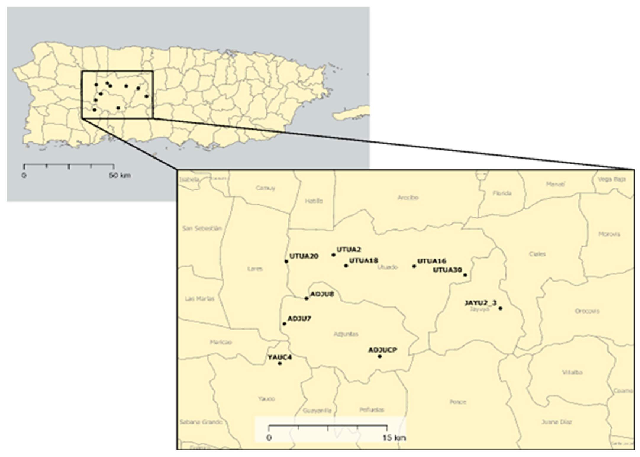
Figure 2.
(a) Depiction of a single-grid flight pattern; (b) Depiction of a double-grid flight pattern.
Figure 2.
(a) Depiction of a single-grid flight pattern; (b) Depiction of a double-grid flight pattern.
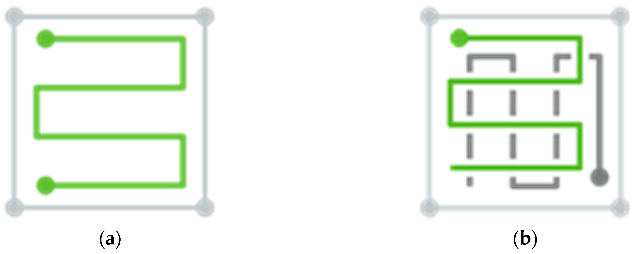
Figure 3.
Example land cover classification of farm UTUA2 using 2022 multispectral imagery. All maps shown are projected in the coordinate system “StatePlane Puerto Rico Virgin Isl FIPS 5200 (Meters),” datum of NAD 1983.
Figure 3.
Example land cover classification of farm UTUA2 using 2022 multispectral imagery. All maps shown are projected in the coordinate system “StatePlane Puerto Rico Virgin Isl FIPS 5200 (Meters),” datum of NAD 1983.
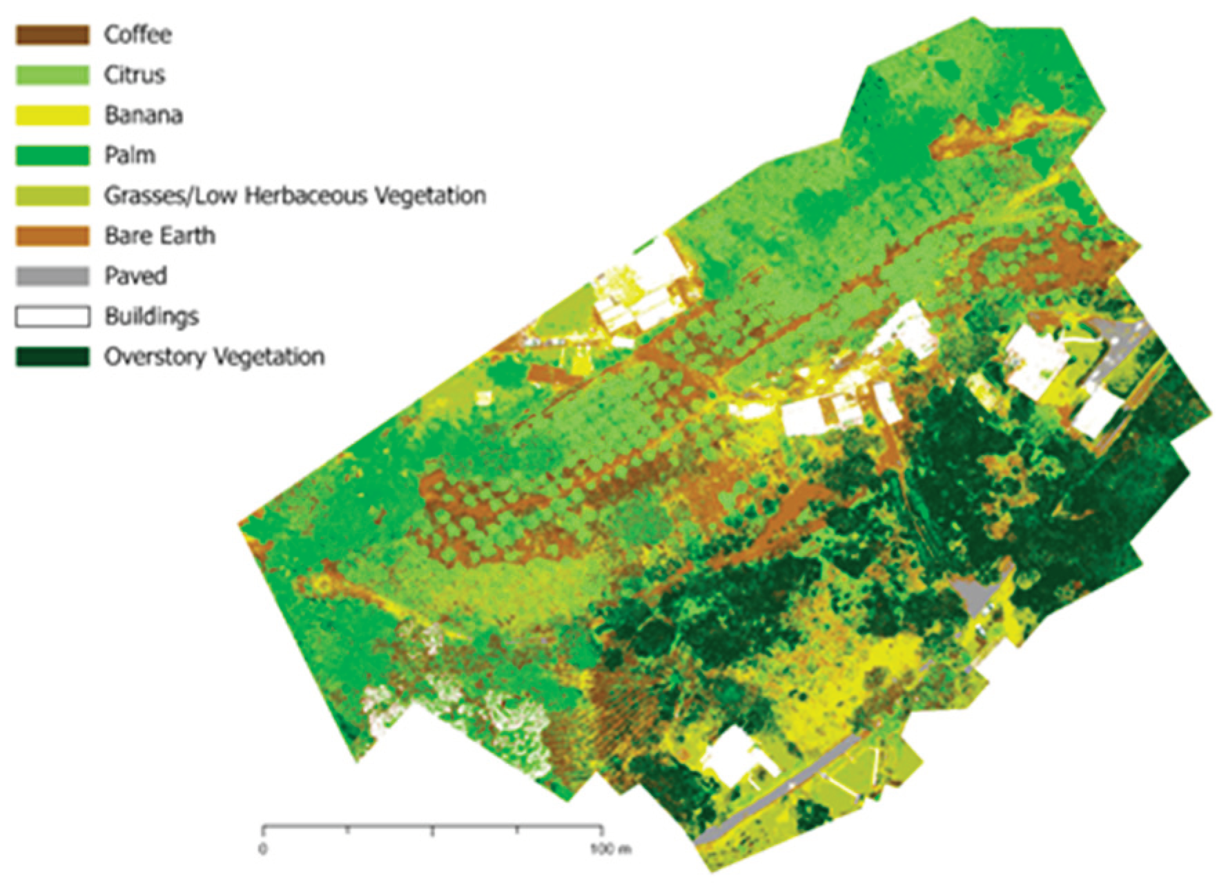
Figure 4.
The spectral profile of vegetation classes for farm UTUA2.
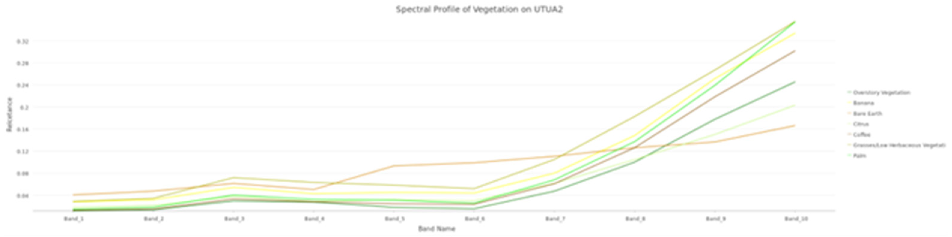
Table 1.
Information on farm size, aspect, slope, and classification based on Moguel and Toledo’s (1999) coffee growing gradient.
Table 1.
Information on farm size, aspect, slope, and classification based on Moguel and Toledo’s (1999) coffee growing gradient.
| Farm | Size (ha) | Aspect | Median Slope (°) | Classification |
| UTUA2 | 1.64 | West-facing | 7 | Commercial polyculture |
| UTUA16 | 0.96 | South-facing | 12 | Traditional polyculture |
| UTUA18 | 2.13 | East-facing | 16 | Traditional polyculture |
| UTUA20 | 1.63 | South-facing | 18 | Commercial polyculture |
| UTUA30 | 0.82 | West-facing | 25 | Traditional polyculture |
| YAUC4 | 2.47 | North-facing | 12 | Traditional polyculture |
| ADJUCP | 3.45 | North-facing | 12 | Commercial polyculture |
| ADJU8 | 41.97 | East-facing | 16 | Shaded monoculture |
| JAYU2_3 | 56.05 | South-facing | 17 | Shaded monoculture |
Table 2.
Spectral band information for the MicaSense RedEdge-MX Dual Camera Imaging System as compared to Sentinel-2A MSI and Landsat 8 OLI.
Table 2.
Spectral band information for the MicaSense RedEdge-MX Dual Camera Imaging System as compared to Sentinel-2A MSI and Landsat 8 OLI.
| Sentinel-2A MSI | Landsat 8 OLI | MicaSense RedEdge-MX Dual Camera Imaging System | |||
| Spectral Region | Wavelength range (nm) | Spectral Region | Wavelength range (nm) | Spectral Region | Wavelength range (nm) |
| Blue | 458–523 | Blue | 435–451 | Blue | 430-458 |
| Green peak | 543–578 | Blue | 452–512 | Blue | 459-491 |
| Red | 650–680 | Green | 533–590 | Green | 524-538 |
| Red edge | 698–713 | Red | 636–673 | Green | 546.5-573.5 |
| Red edge | 733–748 | NIR | 851–879 | Red | 642-658 |
| Red edge | 773–793 | SWIR1 | 1566–1651 | Red | 661-675 |
| NIR | 785–899 | SWIR2 | 2107–2294 | Red Edge | 700-719 |
| NIR narrow | 855–875 | Red Edge | 711-723 | ||
| SWIR | 1565–1655 | Red Edge | 731-749 | ||
| SWIR | 2100–2280 | NIR | 814.5-870.5 | ||
Table 3.
Improved classification iterations applied on 2022 farm imagery.
| Iteration name | Multispectral bands | Principal components | Other layers | Farms layer stack was performed on |
| Iteration A | 1-10 | 一 | 一 | UTUA2, UTUA16, UTUA18, UTUA20, UTUA30, YAUC4, ADJU8, JAYU2 |
| Iteration B | 一 | 1-10 | 一 | UTUA2, UTUA16, UTUA18, UTUA20 |
| Iteration C | 5-7 | 1-3 | 一 | UTUA2, UTUA16, UTUA18 |
| Iteration D | 5-8 | 1-3 | 一 | UTUA20 |
| Iteration E | 5-10 | 1, 2 | 一 | UTUA2 |
| Iteration F | 5-7 | 1-3 | NDVI | UTUA2 |
Table 4.
The number of flights flown for each farm in the 2022 field campaign.
| Farms | Number of flights |
| UTUA2 | 1 |
| UTUA16 | 1 |
| UTUA18 | 1 |
| UTUA20 | 1 |
| UTUA30 | 2 |
| YAUC4 | 1 |
| ADJUCP | 2 |
| ADJU7 | 3 |
| ADJU8 | 7 |
| JAYU2_3 | 8 |
Table 5.
Ground control points collected by year.
| Year | ||||
| Farm | 2021 | 2022 | 2023 | TOTAL |
| UTUA2 | 69 | 112 | 73 | 254 |
| UTUA16 | - | 20 | 52 | 72 |
| UTUA18 | 41 | 32 | 21 | 94 |
| UTUA20 | 49 | 41 | 31 | 121 |
| UTUA30 | 51 | 24 | - | 75 |
| YAUC4 | 51 | 28 | - | 79 |
| ADJU8 | 63 | 44 | 1 | 108 |
| JAYU2_3 | 140 | 63 | 30 | 233 |
| TOTAL | 464 | 364 | 208 | 1036 |
Table 6.
Accuracy of farm classification using 2022 imagery. The table details the overall accuracy of each farm along with Cohen’s Kappa statistic.
Table 6.
Accuracy of farm classification using 2022 imagery. The table details the overall accuracy of each farm along with Cohen’s Kappa statistic.
| Farm | Overall Accuracy (%) | Kappa (𝛋) |
| UTUA2 | 57.0 | 0.463 |
| UTUA16 | 49.4 | 0.369 |
| UTUA18 | 58.4 | 0.447 |
| UTUA18_obj | 36.8 | 0.221 |
| UTUA20 | 52.4 | 0.388 |
| UTUA30 | 51.3 | 0.391 |
| YAUC4 | 74.0 | 0.509 |
| ADJU8 | 53.5 | 0.463 |
| JAYU2_3 | 52.6 | 0.430 |
Table 7.
Content matrix summarizing interview findings.
| Themes | Quote/Example | Research Finding | Subthemes | Relevance to land cover classification map and methodology |
| Utility | “What is the purpose of us seeing this?” | Many farmers were unsure how the classification maps could fit into the farm management but were excited about the maps and being able to keep them. | Beauty | Landcover maps are created with the intention of better understanding the makeup of a given area to enhance land management. However, there were no clear farmer-generated ideas on the implementation of the maps in their own management, nor any motivation to implement the ones suggested by researchers. |
| Novelty | The majority of farmers provided excited exclamations when presented with a map. | Farmers are open to the use of maps and the classification and visuals in their present form. | Pride, Technology | There is still excitement about the prospect of utilizing drone imagery and classifications but there still exists a gap in understanding the applicability of relatively new technology in these contexts. |
| “You can think you know everything. On the contrary, huh. Technology advances, Knowledge is continuous.” | ||||
| Orientation | “I don’t know where it is.” | When relevant personal landmarks were noted, farmers often used them to orient themselves. In the case that they were not present, their absence was noted and farmers then used other points or direction from interviewers to orient themselves. | Movement, Landmarks, Perspectives | In connection to novelty and utility, a lack of orientation means that the imagery or classification maps may not be implemented and may instead become a barrier for farmers engaging with this technology. |
| “Oh, there’s my lake!” or “I let myself be led by the buildings.” | ||||
| Biodiversity | Many farmers noted that other food crops and vegetation were present on the farm but had not been mapped (i.e., peppers, guaraguao trees, smaller citrus, mangoes). | Within diversified farming, there is a wealth of food crops and non-food crops that farmers prioritize. | Food Crops, Land Management | While capturing biodiversity present in diverse agroecosystems is desired, maps created that highlight such diversity may also be overwhelming or imperceivable to those who have not yet had an introduction to this type of imagery. |
| Clarity | “I know the farm, but that’s not exactly it, but it’s not because I really see it there.” | While farmers express wanting representation of the entirety of crops and vegetation, a cursory introduction to the maps in a simplified form aids synthesis of imagery and content. | Digestibility, Simplification | Understanding the audience of a map is a principal element of cartography. In a setting such as this study, creating a simpler iteration may serve as a tool with which to foster connections and understand where to expound upon classifications or tools in the future. |
| Visual representation provided in a concise formatting supported outward expressions of map legibility. | ||||
| Land Management | A farmer speaking to the increased heat noted they needed to plant more plants to shade coffee. | Land management techniques often include practices to address climatic conditions. By diversifying crops, farmers are better shielded from economic downturns and a rapidly changing environment. | Crop Selection, Crop Placement | Land management may inform classifications by creating more targeted areas for ground truthing and testing sites. For example, if a farmer noted that coffee was planted under an area of dense canopy, it may make sense to ground truth the area heavily and test the degree to which the coffee in that area was present in the classification. |
| Farmers intercropped coffee with citrus as a means of protecting the coffee (their primary crop). |
Disclaimer/Publisher’s Note: The statements, opinions and data contained in all publications are solely those of the individual author(s) and contributor(s) and not of MDPI and/or the editor(s). MDPI and/or the editor(s) disclaim responsibility for any injury to people or property resulting from any ideas, methods, instructions or products referred to in the content. |
© 2024 by the authors. Licensee MDPI, Basel, Switzerland. This article is an open access article distributed under the terms and conditions of the Creative Commons Attribution (CC BY) license (http://creativecommons.org/licenses/by/4.0/).
Copyright: This open access article is published under a Creative Commons CC BY 4.0 license, which permit the free download, distribution, and reuse, provided that the author and preprint are cited in any reuse.


