Submitted:
05 March 2024
Posted:
06 March 2024
You are already at the latest version
Abstract
OpenFOAM is a CFD software widely used in both industry and academia. The exaFOAM project aims at enhancing the HPC scalability of OpenFOAM, while identifying its current bottlenecks and proposing ways to overcome them. For the assessment of the software components and the code profiling during the code development, lightweight but significant benchmarks should be used. The answer was to develop microbenchmarks, with a small memory footprint and short runtime. The name microbenchmark does not mean that they have been prepared to be the smallest possible test cases, as they have been developed to fit in a compute node, which usually has dozens of compute cores. The microbenchmarks cover a broad band of applications: incompressible and compressible flow, combustion, viscoelastic flow and adjoint optimisation. All benchmarks are part of the OpenFOAM HPC Technical Committee repository and are fully accessible. The performance using HPC systems with Intel and AMD processors (x86_64 architecture) and Arm processors (aarch64 architecture) have been benchmarked. For the workloads in this study, the AMD processor seems particularly suited resulting in an overall shorter time-to-solution.
Keywords:
CFD
; OpenFOAM
; benchmark
1. Introduction
The CFD software OpenFOAM [1] is widely used both in industry and academia, and had its bottlenecks in current HPC systems identified by the exaFOAM project [2], which aims at overcoming them through algorithmic improvements and enhanced HPC scalability.
To demonstrate the improvements in performance and scalability of OpenFOAM, extreme-scale demonstrators (HPC Grand Challenges) and industrial-ready applications have been prepared. However, these test cases are too computationally expensive to assess the software components and the code profiling during the development phases. To solve this problem, less computationally demanding benchmarks have been derived, called microbenchmarks, with a smaller memory footprint and shorter runtime. The name microbenchmark does not mean that they have been prepared to be the smallest possible test cases, as they have been developed to fit in an HPC compute node, which usually has dozens of compute cores.
The microbenchmarks have been designed to be performance proxies of the HPC Grand Challenges and the industrial test cases, representing the full simulation but demanding far less computational time. All benchmarks are part of the OpenFOAM HPC Technical Committee repository [3] and are publicly available.
This set of benchmarks is built as an open and shared entry point to the OpenFOAM community, which can be used as a reference to compare the solution of different physical problems in different hardware architectures.
2. Materials and Methods
The performance of OpenFOAM on different HPC architectures and processor types has been compared, in particular with the x86_64 and aarch64 architectures. In the case of x86_64, both Intel and AMD processors were employed, while in the case of aarch64, Arm processors were used. Table 1 shows a summary of the HPC architectures and processor types utilized for the tests.
From the collection of microbenchmarks published by the exaFOAM project in the OpenFOAM HPC technical committee repository [3], 11 have been considered in this work, listed in Table 2 along with their solvers and information about grid characteristics.
For completeness, a short description of each microbenchmark follows in the next subsections. The interested reader is pointed to the OpenFOAM HPC Technical Committee repository [3] where the test cases are fully described, along with instructions on how to run them.
2.1. MB1 Cavity 3D
The flow in a cavity, which is driven by the upper cavity boundary (lid), is one of the most basic and widely spread test cases for the CFD programs (see Figure 1). It is easy to set up and validate because of the simple geometry. According to AbdelMigid et. al. [4] the setup has been used by researchers for more than 50 years to benchmark fluid dynamics codes. Available literature on the topic includes numerical experiments for a wide range of computational algorithms and flow regimes, e.g., Ghia et. al. [5] provide comprehensive results for the Reynolds number ranging from 100 to 10 000. In most cases, the numerical setups are 2D whereas experimental measurements are carried out in 3D as performed by Koseff et. al. [6].
The present setup is based on the white paper by Bnà et. al. [7]; thus, scaling results are available.
2.2. MB2 Compressible Starting Square Jet
A high-speed injection of a warm gas (330 K) into a static atmosphere with a slightly lower temperature (300 K) is considered (see Figure 2). For simplicity, the jet fluid enters the atmospheric box through a square inlet (0.0635 m) resolved with a homogeneous structured mesh (no grid stretching). Given the low gas viscosity (1.8 10−5Pa s) and high velocity (364 m/s) of the injected fluid, the jet flow is unsteady and compressible, characterised by high Mach number (>1 locally) and Reynolds number. Non-linear instabilities in the jet shear layer (like Kelvin-Helmholtz), vortexes, pressure waves and a turbulent buoyant plume typically develop with these conditions. In the simulations, the jet fluid, as it enters the atmospheric box, forms a vortex and pushes the static air outwards producing an intense pressure wave followed by smaller transients that propagate radially (see Figure 2).
2.3. MB4 DLR-JHC Burner
The combustion chamber investigated by the DLR Institute of Combustion Technology is simulated. Figure 3 (left) presents the entire structure; detailed information is reported in the literature [9]. A pre-chamber exists below a top vessel. The top vessel is considered in the current analysis; the pre-chamber is neglected. The top of the considered chamber is open. A jet of fuel is introduced in the vessel; the region is initially filled with vitiated air coming from a preliminary combustion process between air and H2 which takes place in the pre-chamber. The vitiated air is accounted as a homogeneous mixture because of the perfect mixing occurring in the pre-chamber. In the top vessel, the hot vitiated air reacts with the injected methane and generates a steady lift flame. Experiments are publicly available from the DLR Institute of Combustion Technology. The LxWxH rectangular-shaped region is three-dimensional. Due to the introduced simplification, a quarter of the domain can be considered; symmetry planes are identified on two of the resulting sides. A small centered nozzle injects the fuel, while air with lean premixed hydrogen combustion products is introduced at the bottom of the mesh in the surrounding region.
2.4. MB5 ERCOFTAC Conical Diffuser
The case stems originally from ERCOFTAC. A detailed description is available [10] and experimental data [11] as well. A diffuser is designed to reduce the flow velocity and therefore increase the fluid pressure without causing significant pressure loss, see Figure 4. This is done by increasing the cross-section area, e.g., by introducing a conical segment. The latter is characterized by a so-called divergence angle, which is the angle between the opposite walls in the axial cross-section through the conical part. Due to this geometry, the flow tends to separate at the diffuser wall, which is undesirable since it causes losses. However, the behavior can be counteracted by the inclusion of a swirling flow component in the flow entering the diffuser. But if the swirl is too strong a recirculation along the center axis occurs, which reduces the pressure recovery.
2.5. MB6 Two Cylinders in Line
This microbenchmark case deals with the flow around two equal-sized cylinders in tandem (in-line) arrangement [13,14]. In this benchmark, a von Karman vortex street appears downstream of the cylinders when the spacing L between them (diacenter) is greater than , where D is the cylinder diameter [13], see Figure 5. Its goal is to showcase the memory savings when using a (lossy) compression scheme for computing sensitivity derivatives for unsteady flows when compared with the full storage of the flow time history. When used with unsteady flows, the adjoint equations are integrated backward in time, requiring the instantaneous flow fields to be available at each time step of the adjoint solver, which noticeably increases storage requirements in large-scale problems. To avoid extreme treatments, such as the full storage of the computed flow fields or their re-computation from scratch during the solution of the adjoint equations and to reduce the re-evaluation overhead incurred by the widely used check-pointing technique [15], lossy compression techniques are be used. Using lossy compression, the re-computation cost is expected to be reduced by efficiently compressing the check-points, so that more can fit within the available memory, or even eliminate the need for check-pointing (and flow re-computations) if the entire compressed flow series can be stored in memory. The compression strategies will be assessed based on their effectiveness in data reduction, computational overhead, and accuracy of the computed sensitivity derivatives.
2.6. MB8 Rotating Wheel
This microbenchmark aims to represent an industrial application on a small scale using the arbitrary mesh interface (i.e. ACMI) in OpenFOAM. The case consists of a single isolated rotating front left wheel of the DrivAer full-scale car model in the variant introduced by Ford [16], see Figure 6. The CAD data was taken from case 2 of the 2nd automotive CFD prediction workshop [17] and the parts used for this microbenchmark are shown in Figure 7. The positioning of the wheel axis is inherited from the full-scale case and indicated in Figure 6. The domain inlet is positioned at x=-2500 mm, such that the domain lengths upstream and downstream of the wheel are approximately 3.4D and 9.7D with D being the outer tire diameter. The domain size is chosen arbitrarily but ensures adequate distance to boundaries for numerical stability and resolution of the turbulent flow downstream of the wheel.
2.7. MB9 High-Lift Airfoil
The MB9 microbenchmark is intended for preparatory work building up to the simulation of the exaFOAM Grand Challenge test case of the High Lift Common Research Model (CRM-HL) [18], a full aircraft configuration with deployed high-lift devices using wall-modelled LES (WMLES). MB9 is a two-dimensional, three-element high-lift wing configuration. The configuration is simulated with the scale-resolving IDDES model [19], which exhibits WMLES functionality in regions of resolved near-wall turbulence (e.g. on the suction side of the main element). After a review of various public-domain test cases, the 30P30N case was selected, which was studied extensively with WMLES in the 4th AIAA CFD High Lift Prediction Workshop (HLPW-4) and has experimental data available [20]. The geometry of the test case is shown in Figure 8.
2.8. MB11 Pitz&Daily Combustor
The case is based on the experiment carried out by Pitz and Daily [21], who measured a combustion flow formed at a backward-facing step. The goal of the work was to study the turbulent shear layer during a combustion process in conditions similar to those of industrial and aircraft gas turbine combustors. The premixed combustion is stabilized by recirculation of hot products which are mixed with cold reactants in a turbulent shear layer. The setup with a backward-facing step is one of the simplest configurations reproducing these conditions.
The dimensions used in the numerical setup are kept the same as in the OpenFOAM tutorial cases, however, in a 3D configuration. (see Figure 9). These deviate from the geometry described in the experimental setup by several mm. Furthermore, there are no dimensions of the contraction section available in the original paper [21]. It is assumed that these deviations do not introduce a significant influence on the final results. An additional geometry feature that matters is the ramp upstream of the test section. Calculations with a short straight inlet section resulted in a stable flow demonstrating no fluctuations. This is probably due to the insufficient development of the boundary layer up to the edge of the step. Thus, the inclusion of the ramp is essential for the results.
2.9. MB12 Model Wind Farm
Large-eddy simulations (LES) are a prominent tool for performing high-fidelity simulations of wind turbine wakes and wind farm flows. LES can capture the three-dimensional unsteady character of the flow around wind turbines and the wake flow interaction that occurs in wind farms. However, the influence of the wind turbines on the flow has to be modeled, as is still not feasible to use body-fitted meshes or immersed boundary methods to fully resolve the blades.
To study the turbine wakes generated by wind turbines, LES simulations using the Actuator Disc Model (ADM) are compared with the wind tunnel experimental data of the Saint Anthony Falls Laboratory at the University of Minnesota. Two complementary setups are studied: a single wind turbine, described in references [22,23], and a wind farm with 30 wind turbines, described in references [24,25]. Figure 10 shows a plot of the wind farm simulation, along with the position of the 30 wind turbines that form the wind farm.
2.10. MB17 1D Aeroacoustic Wave Train
This is the exact complement to the microbenchmark MB15 (1D Hydroacoustics wave train), which is not shown in this work. The aeroacoustic wave train is applied to the aerodynamics industry, and is relevant to the automotive, aerospace, energy, and environmental industry sectors. The important distinction with MB15 is the difference in scales (frequency and wavelength of aeroacoustics versus hydroacoustics) which determine the domain extent, and OpenFOAM solver in respect of equation of state (ideal gas instead of liquid compressibility).
A 2.5m length one-dimensional domain is used for wave propagation at 3000 Hz (also corresponding to a typical frequency of aeroacoustics excitation, and within the peak human hearing range). The working fluid is air and the compressible ideal-gas equation of state is solved to simulate wave propagation. Acoustics damping is used to suppress spurious numerical artifacts and boundary wave reflection.
2.11. MB19 Viscoelastic Polymer Melt Flow
The long computational time required to perform a numerical simulation of profile extrusion forming, considering realistic (viscoelastic) constitutive models, is incompatible with usual industrial requirements. This microbenchmark case study represents a typical profile extrusion problem and aims at assessing the solver viscoelasticFluidFoam available in foam-extend 4.1. The geometry resembles a typical profile extrusion die, with a circular inlet with a radius of 12.5mm which connects to the extruder, and a rectangular outlet that allows manufacturing a profile with a rectangular cross-section of 15x2 mm. The middle of the channel comprises a convergent zone, which performs the transition between the circular inlet and the rectangular outlet. As illustrated in Figure 11, due to symmetry, just a quarter of the geometry is considered for the numerical studies.
3. Results
The tests have been performed using the HPC architectures reported in Table 1. From the 19 microbenchmarks (MBs) provided by the exaFOAM project [2], 11 MBs have been selected (see Table 2). OpenFOAM has specific solvers for a class of physical problems to solve, and they have been chosen due to their importance for industrial and academic applications. Another parameter taken into account in the selection of MBs was the size of the grid. Since the MBs were run on one node using from 2 to 32 MPI ranks, a necessary condition was that the size of the problem should fit on the node memory and the computation could be carried out in a reasonable time on the smallest number of processors considered.
The majority of the benchmark runs were performed with OpenFOAM version v2212, only MB19 used the viscoelasticFluidFoam solver from foam-extend 4.1. Both versions were compiled with the GNU Compiler Collection version 8.5.0 and OpenMPI version 4.1.4. Figure 12 shows the execution time per time step or iteration versus the number of ranks (MPI tasks) for the different MBs and architectures considered. The execution time was computed excluding the first time step or iteration, as often it includes initialization operations. Each numerical experiment was repeated five times and the reported execution time is the average. By observing the results of Figure 12, it can be noticed that the execution time decreases by increasing the number of ranks. This occurs in general for all MBs and architectures with few exceptions. In the case of MB1, the execution time on x86_64 architectures decreases up to 24 cores, but then it slightly increases when running on 32 cores. A similar trend is observed on AMD for MB2, MB11, MB12, and MB19, and on Arm for MB11. Somehow unexpected behavior is obtained on AMD for MB4 and on ARM for MB5. In the first case, the execution time decreases from 2 to 8 processors, but then when using 16 and 24 processors a longer execution time is obtained. In the latter case, the execution time with 8 or 16 ranks is approximately the same. Figure 12 also indicates that when few ranks (< 8) are launched, better performance in terms of execution time per iteration is obtained on AMD, where for some MBs the execution time is almost half of the other architectures. Differences tend to be less evident when employing larger numbers of ranks. Another consideration is that the performance, in terms of absolute execution time, is comparable for most MBs using Intel and Arm processors (x86_64 and aarch64 architectures).
The strong scaling speedup (Figure 13) and efficiency (Figure 14) on the different node types have been calculated based on the data collected on the execution time. Several MBs show superlinear speedups on x86_64 architectures with efficiency values that exceed 1 (MB1, 2, 4, 5, 8, 9, 11, 12 and 19) especially when moving from 2 to 4 or 8 cores. This phenomenon is more pronounced on the AMD processor. When using Arm processors, the efficiency exceeds 1 only in the case of MB9. The reason behind the superlinearity is currently being investigated. One hypothesis is that the larger L3 cache of the AMD CPU (128MB for AMD, 22MB for Intel and 4MB for Arm) promotes this behavior.
For all the MBs, we observe a departure from the ideal speedup with efficiency often dropping under 50% when launching more than 8 ranks. OpenFOAM is a well-known memory-bound application, therefore, when reaching the memory bandwidth saturation, launching more MPI tasks does not provide many benefits, as the CPUs are still waiting for data. In general, the x86_64 architectures seem to show better parallel efficiency on all the MBs and up to a larger number of cores, with few exceptions.
Finally, Figure 15 reports the FVOPS (Finite VOlumes solved Per Second) metric [26] for the same numerical experiments. This metric is defined as the number of finite volume elements in the grid divided by the execution time of a time step or iteration. The FVOPS metric depends on all parameters of the simulation, including grid size, partitioning, parallel efficiency, type of solver, and number of variables being solved. However, with fixed parameters, this metric allows the direct comparison of the performance on different systems, even with different grid sizes. The plots in Figure 15 show in many cases local maxima which indicates the optimal number of grid points per core per MB and architecture. It is interesting to notice that these local maxima occur at different values of grid element per rank when utilizing different processor types.
To facilitate a direct comparison of the performance using the different architectures, Figure 16 shows the same results as Figure 15 using box plots summing up the results for all grid sizes for each MB and architecture. The difference in performance using different test cases becomes evident. Figure 15 and Figure 16 also corroborate that the studied MBs seem particularly suited for AMD processors, with which shorter time-to-solution values were recorded.
4. Conclusions
A series of microbenchmarks (MBs) developed by the exaFOAM project has been introduced, having a broad band of applications: incompressible and compressible flow, combustion, viscoelastic flow and adjoint optimization. The MBs have a relatively small memory footprint and short runtime, making them suitable to fill an HPC compute node and work as performance proxies of larger simulations.
Processors from Intel and AMD (x86_64 architecture) and Arm (aarch64 architecture) have been used. The Intel and Arm systems provided similar performance, despite the different architectures. However, the AMD processor seems particularly suited for the workloads in this study, with an overall shorter time-to-solution.
The microbenchmarks are published in the OpenFOAM HPC Committee repository [3] to serve as benchmarks of different physical problems in various hardware architectures.
Author Contributions
Conceptualization, Flavio Galeazzo and Marta Garcia-Gasulla; Funding acquisition, Marta Garcia-Gasulla, Daniele Gregori and Andreas Ruopp; Investigation, Elisabetta Boella, Josep Pocurull, Sergey Lesnik, Henrik Rusche, Simone Bnà, Matteo Cerminara, Federico Brogi and Filippo Marchetti; Methodology, Flavio Galeazzo; Resources, Andreas Ruopp; Writing – original draft, Flavio Galeazzo and Elisabetta Boella; Writing – review & editing, Marta Garcia-Gasulla and R. Gregor Weiß. All authors have read and agreed to the published version of the manuscript.
Funding
This work is carried out in the scope of the exaFOAM project, which has received funding from the German Federal Ministry of Education and Research and the European High-Performance Computing Joint Undertaking (JU) under grant agreements No 16HPC024 and No 956416, respectively. The JU receives support from the European Union’s Horizon 2020 research and innovation programme and France, Germany, Spain, Italy, Croatia, Greece, and Portugal.
Data Availability Statement
All microbenchmarks are published in the OpenFOAM HPC Committee repository [3].
Acknowledgments
The following contributions are acknowledged: Federico Ghioldi and Federico Piscaglia for MB4; Andreas-Stefanos Margetis, Evangelos Papoutsis-Kiachagias and Kyriakos Giannakoglou for MB6; Julius Bergmann, Hendrik Hetmann and Felix Kramer for MB8 and MB9; Ricardo Costa, Bruno Martins, Gabriel Marcos Magalhães and João Miguel Nóbrega for MB19.
Conflicts of Interest
The authors declare no conflicts of interest.
Abbreviations
The following abbreviations are used in this manuscript:
| ACMI | Arbitrarily Coupled Mesh Interface |
| ADM | Actuator Disk Model |
| BM | blockMesh |
| CAD | Computer Aided Design |
| CFD | Computational Fluid Dynamics |
| CFM | cfMesh |
| DLR | Deutsches Zentrum für Luft- und Raumfahrt |
| ERCOFTAC | European Research Community on Flow, Turbulence and Combustion |
| HPC | High-performance computing |
| MBs | Microbenchmarks |
| SHM | snappyHexMesh |
References
- H. G. Weller, G. Tabor, H. Jasak, and C. Fureby. A tensorial approach to computational continuum mechanics using object orientated techniques. Comput. Phys. 1998, 12, 620–631. [Google Scholar] [CrossRef]
- exaFOAM project website https://exafoam.
- OpenFOAM HPC Committee code repository https://develop.openfoam.com/committees/hpc/-/tree/develop/.
- AbdelMigid, T. A. , Saqr, K. M., Kotb, M. A., Aboelfarag, A. A. Revisiting the lid-driven cavity flow problem: Review and new steady state benchmarking results using GPU accelerated code. Alex. Eng. J. 2017, 56, 123–135. [Google Scholar] [CrossRef]
- Ghia, U. K. N. G. , Ghia, K. N., Shin, C. T. High-Re solutions for incompressible flow using the Navier-Stokes equations and a multigrid method. J. Comput. Phys. 1982, 48, 387–411. [Google Scholar] [CrossRef]
- Koseff, J.R.; Street, R.L. (1985). Erratum: The Lid-Driven Cavity Flow: A Synthesis of Qualitative and Quantitative Observations. J. Fluids Eng. 1984, 106, 390–398. [Google Scholar] [CrossRef]
- PETSc4FOAM A Library to plug-in PETSc into the OpenFOAM Framework, Simone Bna, Ivan Spisso, Mark Olesen, Giacomo Rossi.
- Huang, T. , Lim, H. C. Simulation of Lid-Driven Cavity Flow with Internal Circular Obstacles. Appl. Sci. 2020, 10, 4583. [Google Scholar] [CrossRef]
- A. Fiolitakis and C. M. Arndt. Transported PDF simulation of auto-ignition of a turbulent methane jet in a hot, vitiated coflow. Combust. Theory Model. 2020, 24, 326–361. [Google Scholar] [CrossRef]
- ERCOFTAC Swirling diffuser flow https://www.kbwiki.ercoftac.org/w/index.php?title=UFR_4-06_Description.
- Classic Collection Database http://cfd.mace.manchester.ac.uk/ercoftac/doku.php?id=cases:case060&s[]=conical.
- CC BY-NC-SA 4.0 license https://creativecommons.org/licenses/by-nc-sa/4.
- Dehkordi, B. , Moghaddam, H., Jafari, H. Numerical Simulation of Flow Over Two Circular Cylinders in Tandem Arrangement. J. Hydrodyn. Ser. B 2011, 23, 114–126. [Google Scholar] [CrossRef]
- Mittal, S. , Kumar, V., Raghuvanshi, A. Unsteady incompressible flows past two cylinders in tandem and staggered arrangements. Int. J. Numer. Methods Fluids 1997, 25, 1315–1344. [Google Scholar] [CrossRef]
- Griewank, A. , Walther, A. Algorithm 799: Revolve: An implementation of checkpointing for the reverse or adjoint mode of computational differentiation. Acm Trans. Math. Softw. 2000, 26, 19–45. [Google Scholar] [CrossRef]
- Hupertz, B. , Chalupa, K., Krueger, L., Howard, K., Glueck, H.-D., Lewington, N., . . . Shin, Y.-s. On the Aerodynamics of the Notchback Open Cooling DrivAer: A Detailed Investigation of Wind Tunnel Data for Improved Correlation and Reference. SAE Int. J. Adv. Curr. Prac. Mobil. 2021, 3, 1726–1747. [Google Scholar] [CrossRef]
- 4th Automotive CFD Prediction Workshop https://autocfd.eng.ox.ac.
- AIAA Paper 2020–2771. [CrossRef]
- M. Shur, P. Spalart, M. Strelets, A. Travin. A hybrid RANS-LES approach with delayed-DES and wall-modelled LES capabilities. Int. J. Heat Fluid Flow 2008, 29, 1638–1649. [Google Scholar] [CrossRef]
- V. Chin, D. V. Chin, D. Peters, F. Spaid, R. McGhee (1993): Flowfield measurements about a multi-element airfoil at high Reynolds numbers. AIAA Paper 1993-3137. [CrossRef]
- Pitz, R. W. , Daily, J. W. Combustion in a turbulent mixing layer formed at a rearward-facing step. AIAA J. 1983, 21, 1565–1570. [Google Scholar] [CrossRef]
- L.P. Chamorro and F. Porté-Agel, Effects of thermal stability and incoming boundary-layer flow characteristics on wind turbine wakes: A wind-tunnel study, Bound.-Layer Meteorol. 2010, 136, 515. [CrossRef]
- Wu, Y. T. , and Porté-Agel, F. Large-Eddy Simulation of Wind-Turbine Wakes: Evaluation of Turbine Parametrisations. Bound.-Layer Meteorol. 2011, 138, 345–366. [Google Scholar] [CrossRef]
- L. P. Chamorro and F. Porté-Agel, Turbulent flow inside and above a wind farm: A wind-tunnel study. Energies 2011, 4, 1916–1936. [Google Scholar] [CrossRef]
- Wu, Y.-T. , and Porté-Agel, F. Simulation of Turbulent Flow Inside and Above Wind Farms: Model Validation and Layout Effects. Bound.-Layer Meteorol. 2013, 146, 181–205. [Google Scholar] [CrossRef]
- Galeazzo, F. C. C. , Weiß, G. R. and Ruopp, A. Understanding Superlinear Speedup in Current HPC Architectures. 18th OpenFOAM Workshop (OFW18), Genova, Italy, 11-. 14 July.
Figure 1.
Volume rendering colored by velocity magnitude.
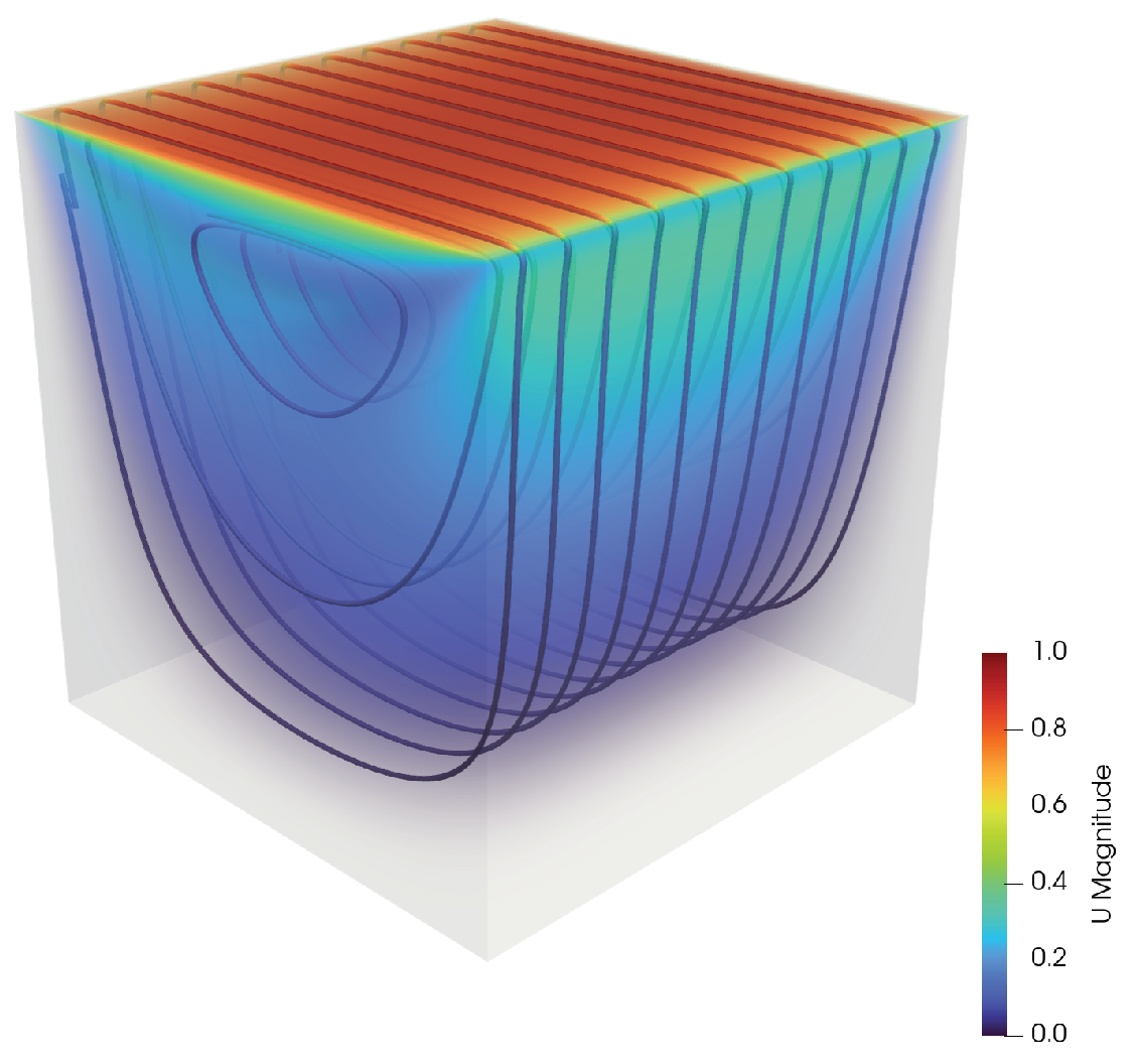
Figure 2.
Screenshot of LES simulation of the supersonic starting jet performed with rhoPimpleFOAM solver. The magnitude of the velocity field (in color) and pressure fluctuations (black and white) are shown.
Figure 2.
Screenshot of LES simulation of the supersonic starting jet performed with rhoPimpleFOAM solver. The magnitude of the velocity field (in color) and pressure fluctuations (black and white) are shown.
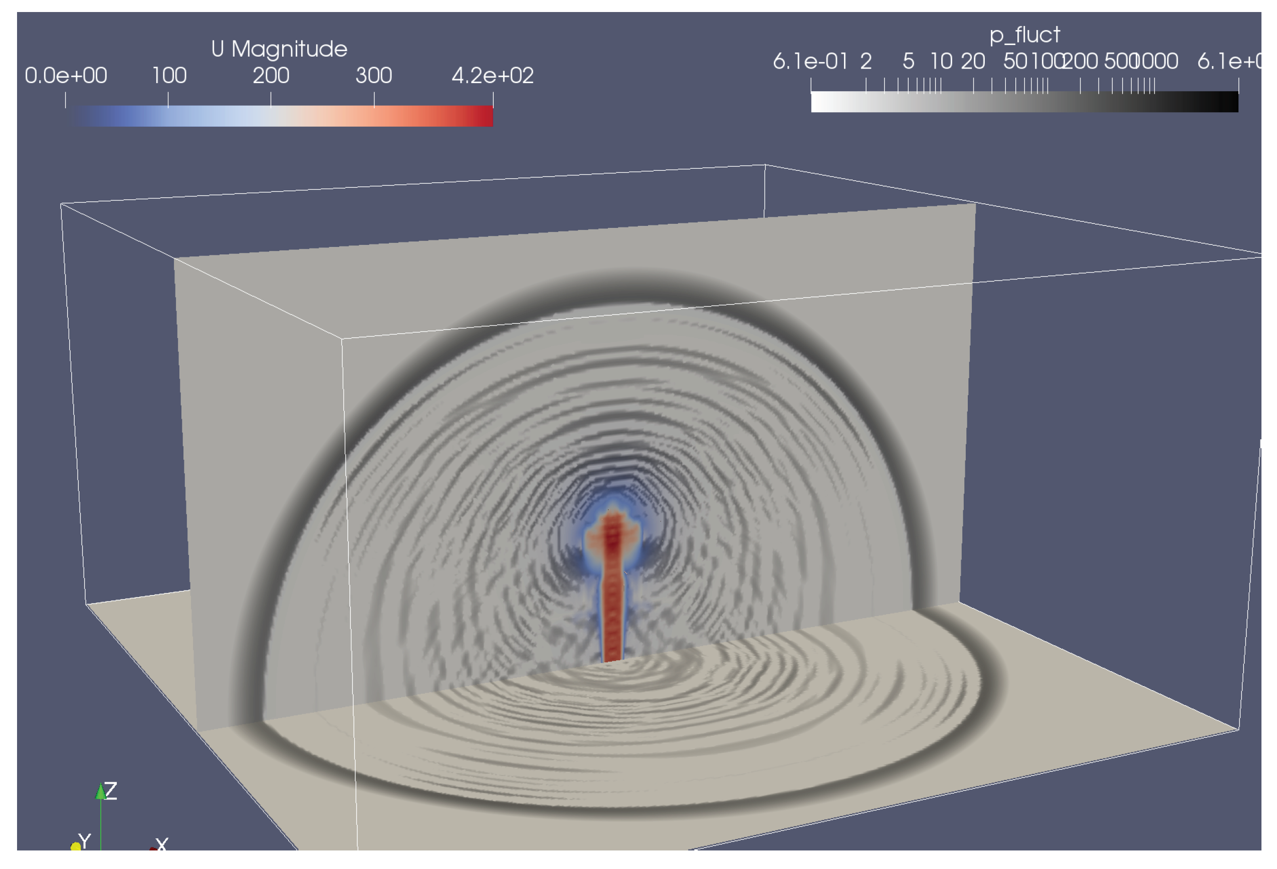
Figure 3.
The three-dimensional geometry is based on the information available from the literature. Simplifications are introduced to account for one-quarter of the entire top construction due to symmetry planes.
Figure 3.
The three-dimensional geometry is based on the information available from the literature. Simplifications are introduced to account for one-quarter of the entire top construction due to symmetry planes.
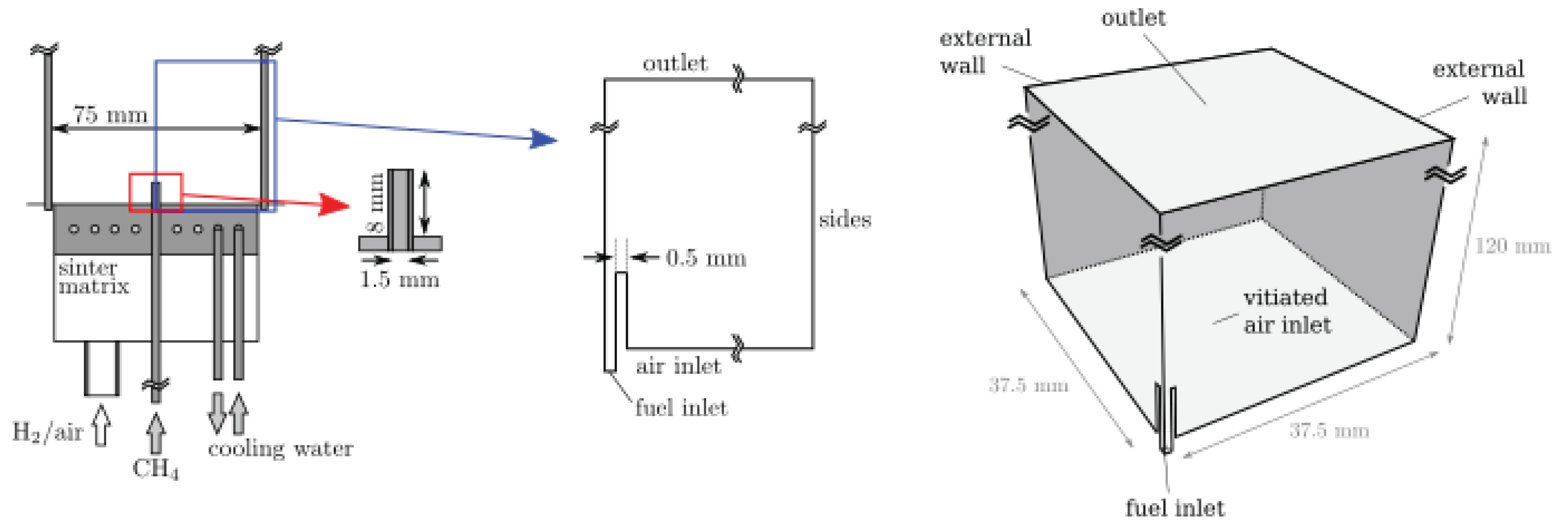
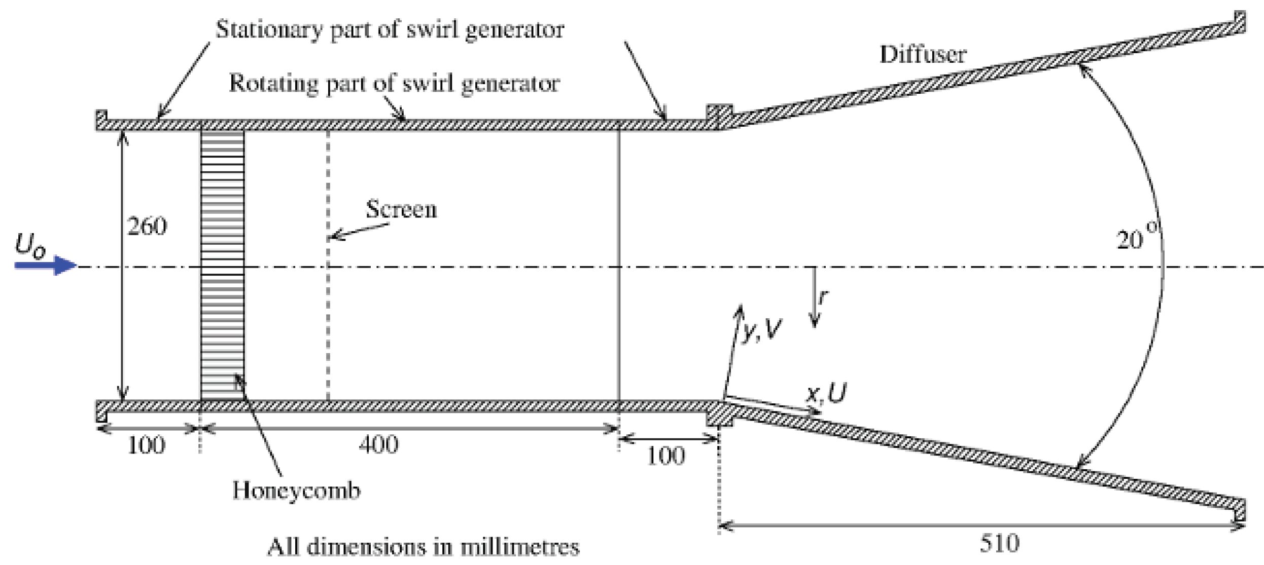
Figure 5.
Two cylinders in tandem with an instantaneous depiction of the magnitude of the primal velocity.
Figure 5.
Two cylinders in tandem with an instantaneous depiction of the magnitude of the primal velocity.
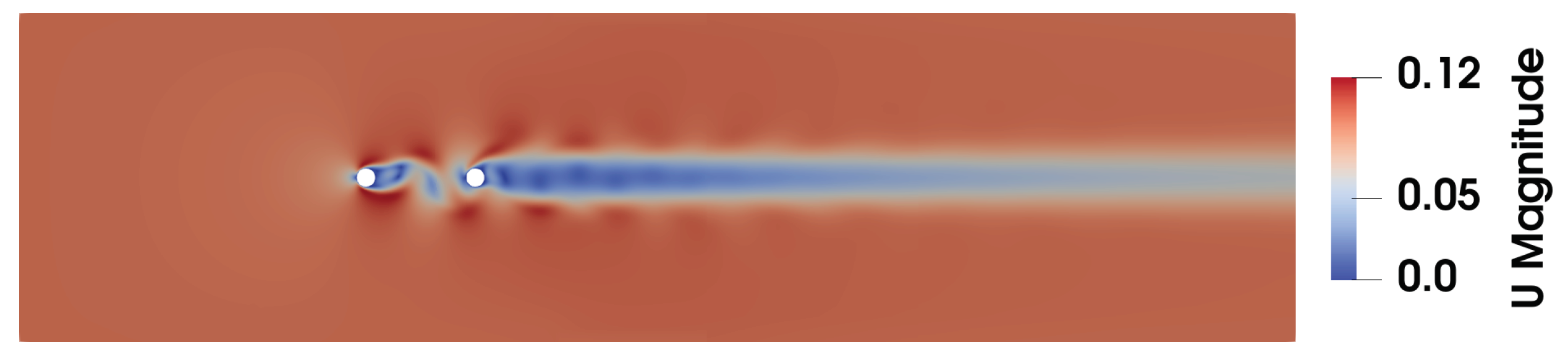
Figure 6.
DrivAer geometry with the indication of the selected wheel.
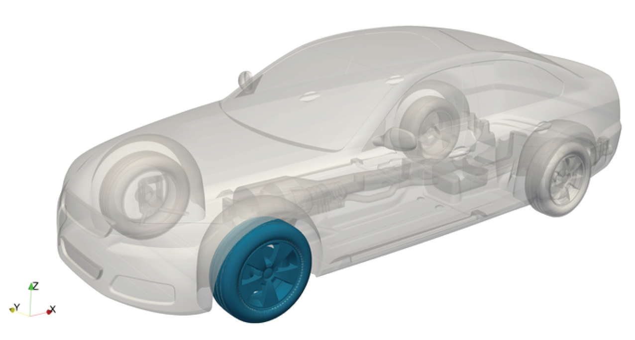
Figure 7.
Selected wheel parts: The tire (grey), the rim (blue), and the brake disc (green).
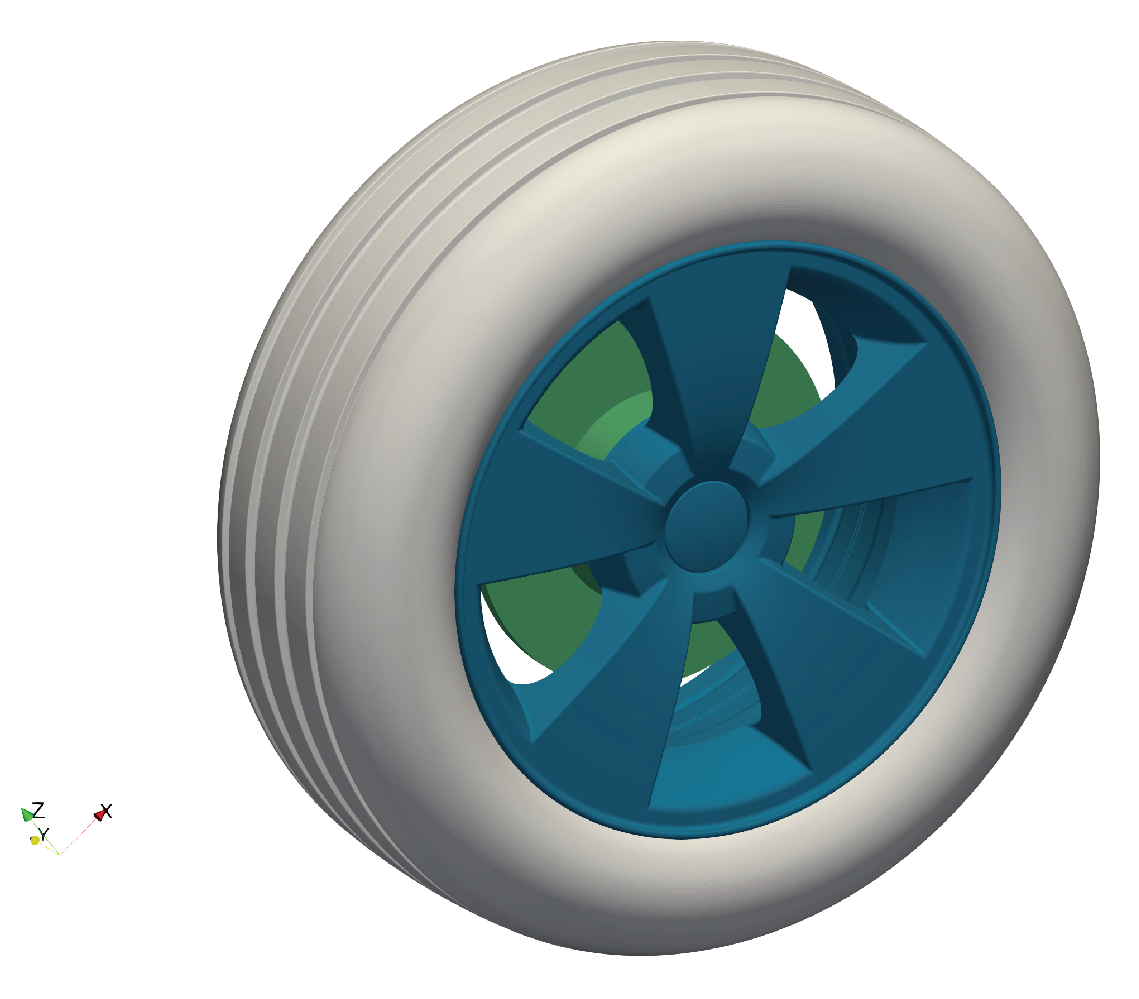
Figure 8.
Geometry of the 30P30N three-element configuration.

Figure 9.
Geometry of the numerical setup. The dimensions are in mm.
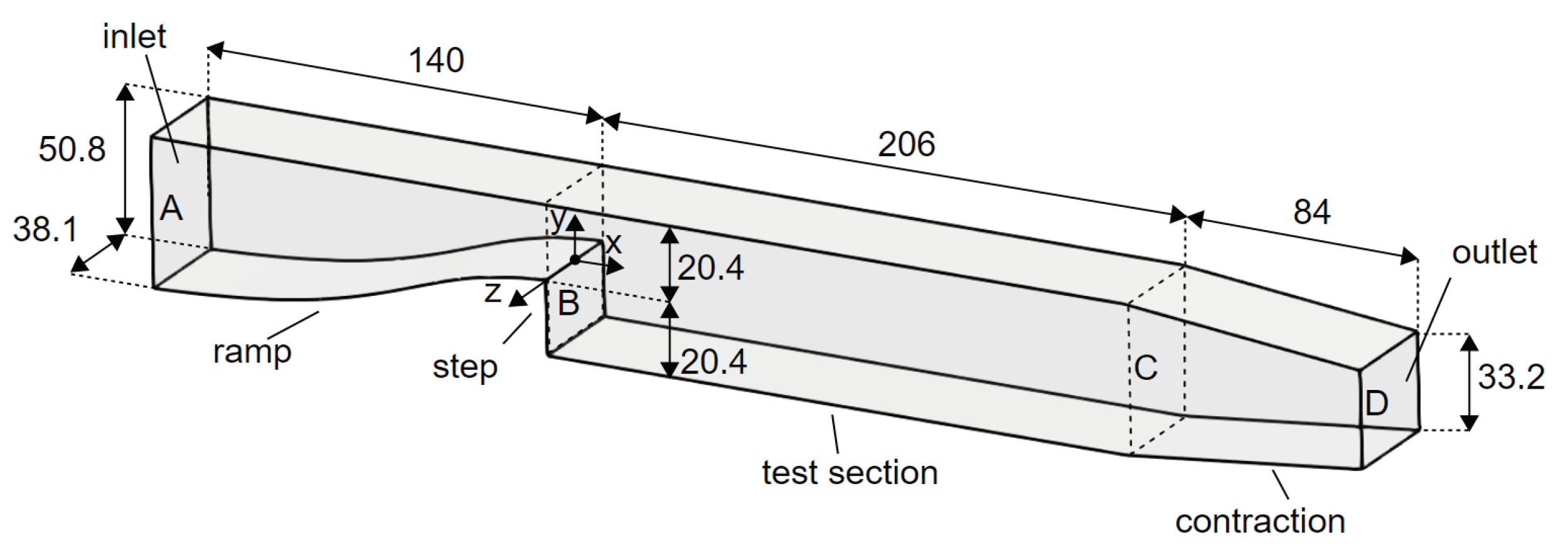
Figure 10.
Contour plot of the velocity magnitude, wind farm.
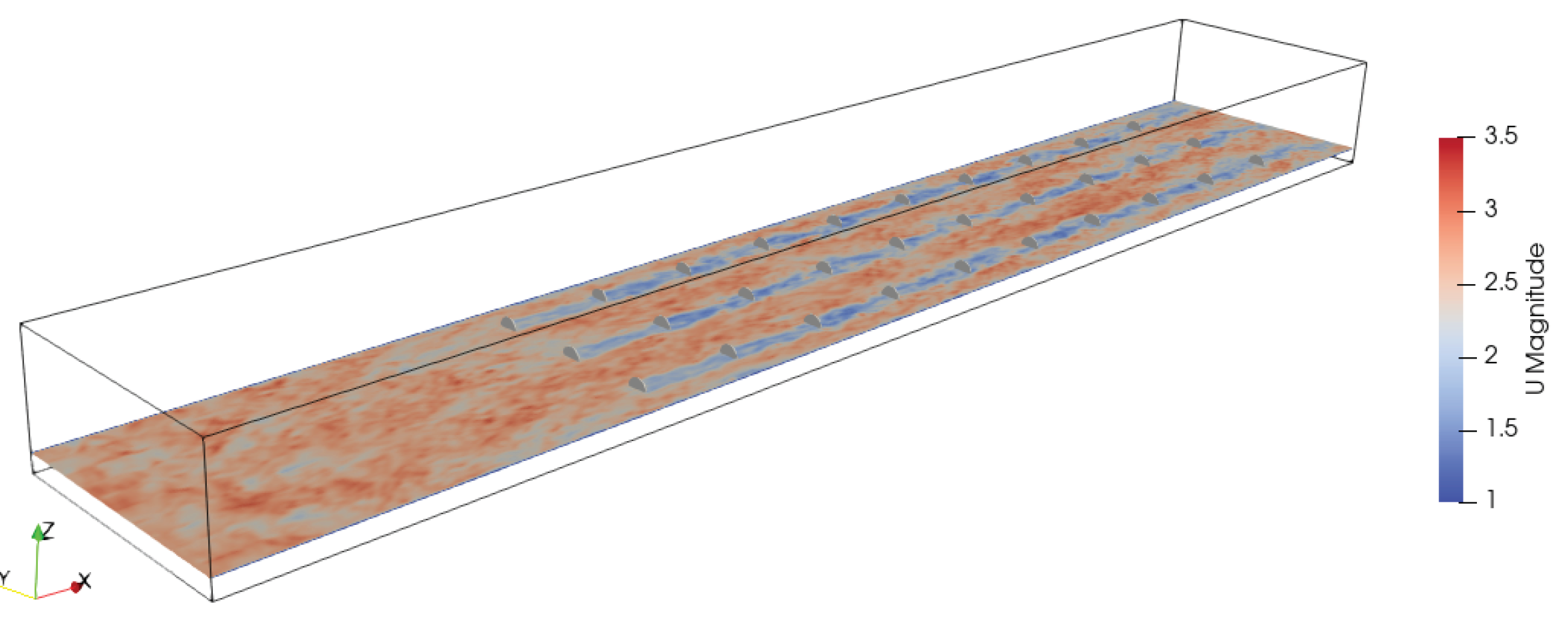
Figure 11.
MB19 geometry.
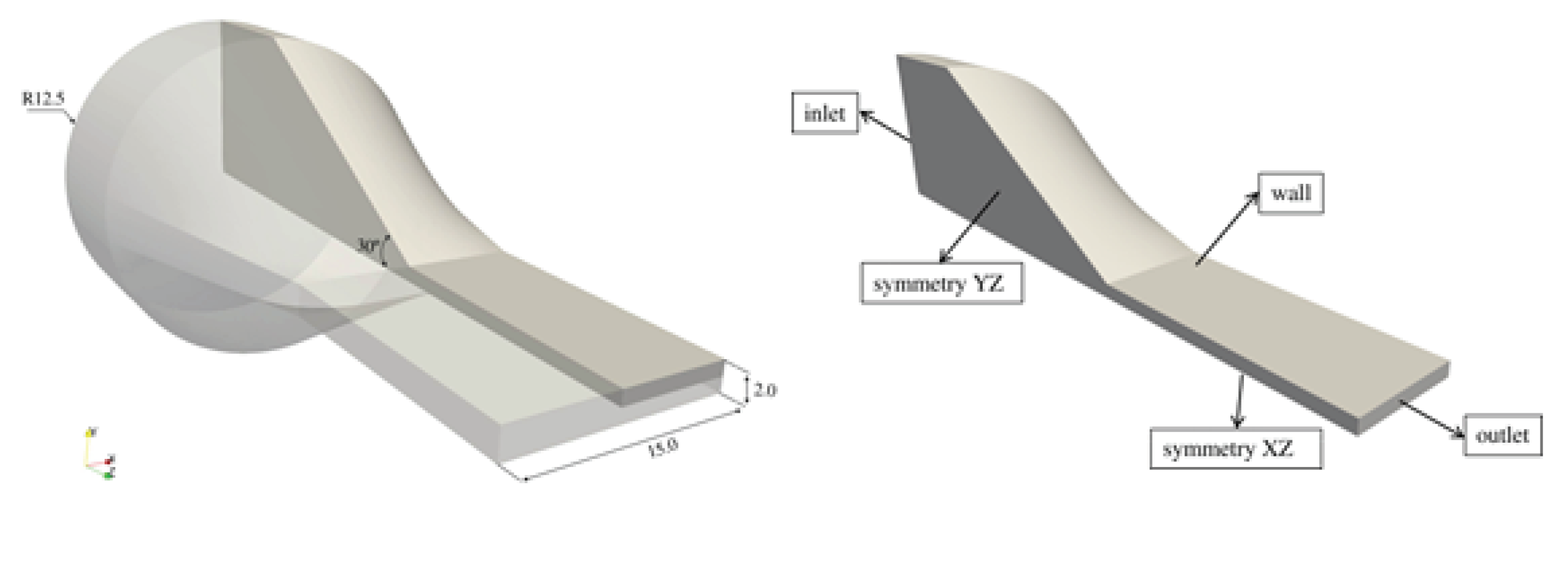
Figure 12.
Execution time per OpenFOAM iteration vs number of ranks (MPI tasks) for different microbenchmarks.
Figure 12.
Execution time per OpenFOAM iteration vs number of ranks (MPI tasks) for different microbenchmarks.
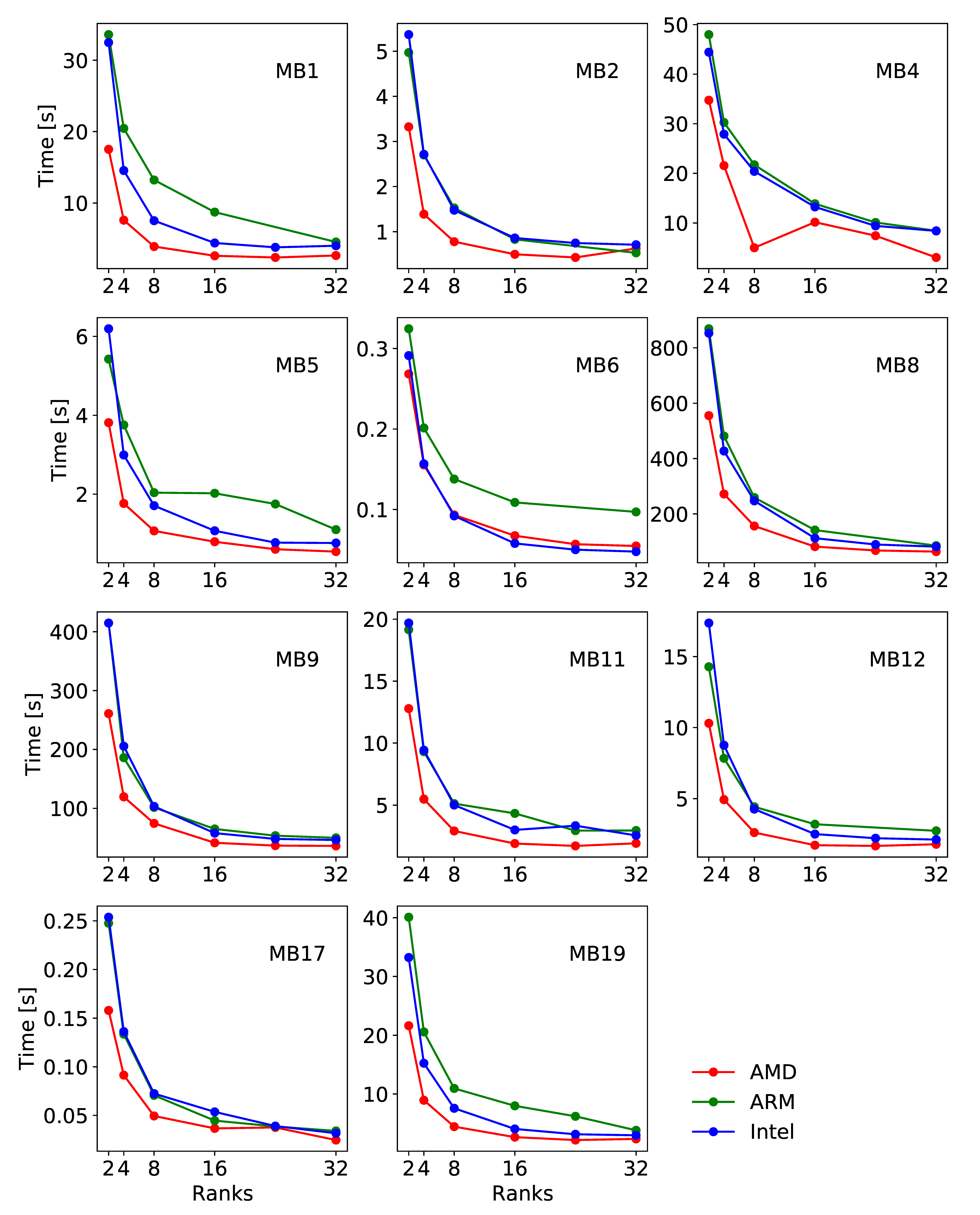
Figure 13.
Speedup for different microbenchmarks in OpenFOAM strong scaling tests.
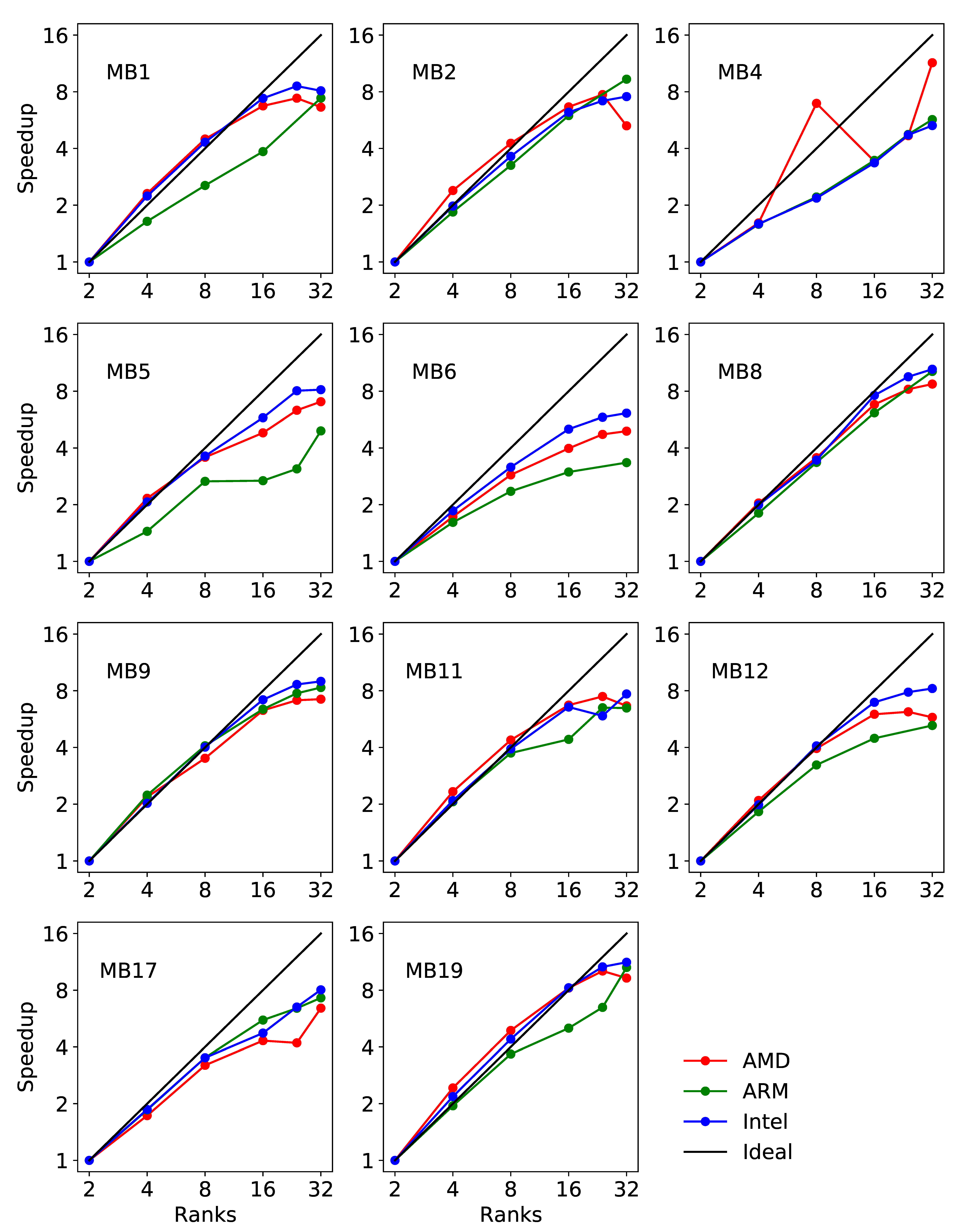
Figure 14.
Efficiency for different microbenchmarks in OpenFOAM strong scaling tests. The black line represents the ideal efficiency.
Figure 14.
Efficiency for different microbenchmarks in OpenFOAM strong scaling tests. The black line represents the ideal efficiency.
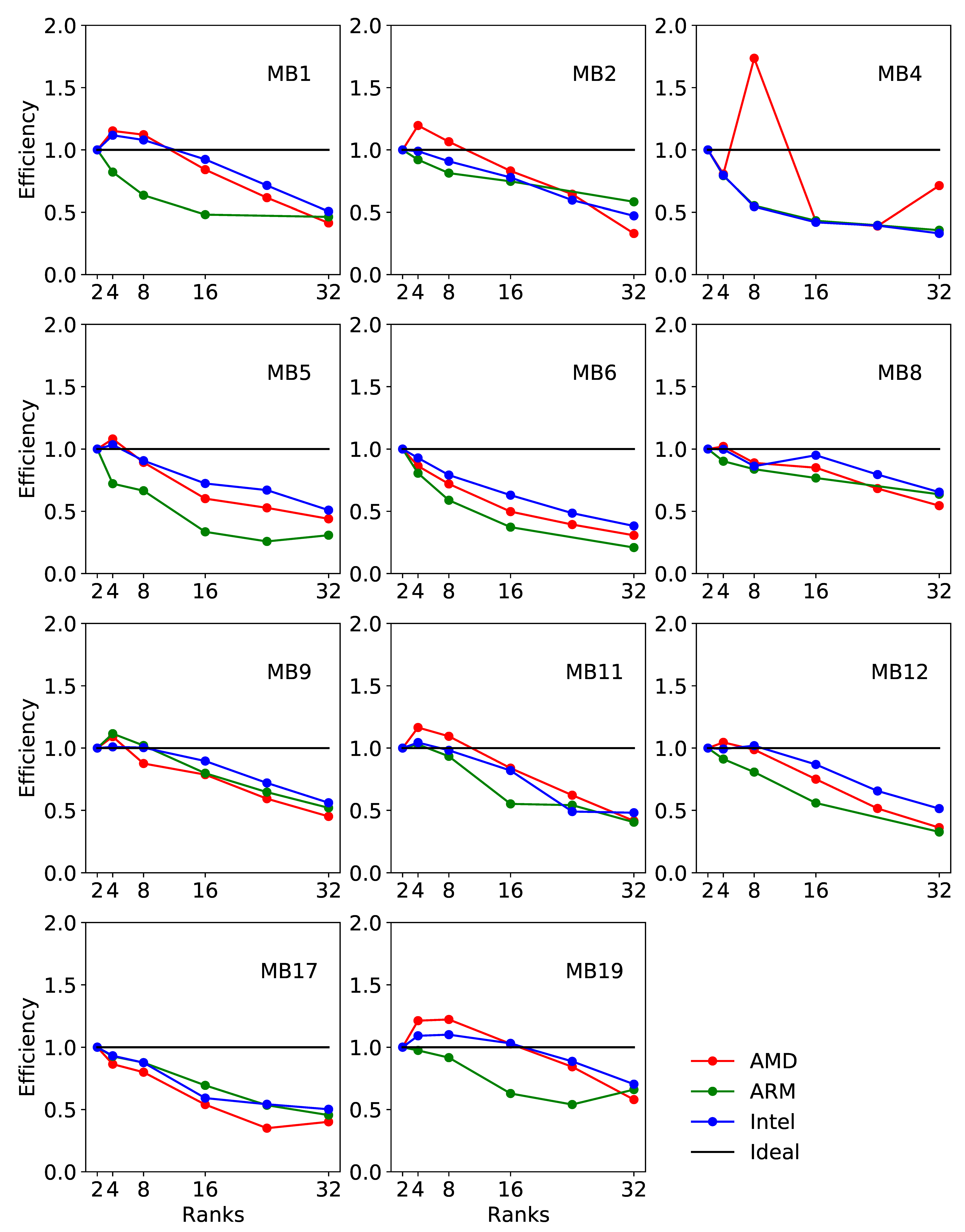
Figure 15.
FVOPS metric vs grid elements per rank for different microbenchmarks. The black line represents the ideal efficiency.
Figure 15.
FVOPS metric vs grid elements per rank for different microbenchmarks. The black line represents the ideal efficiency.
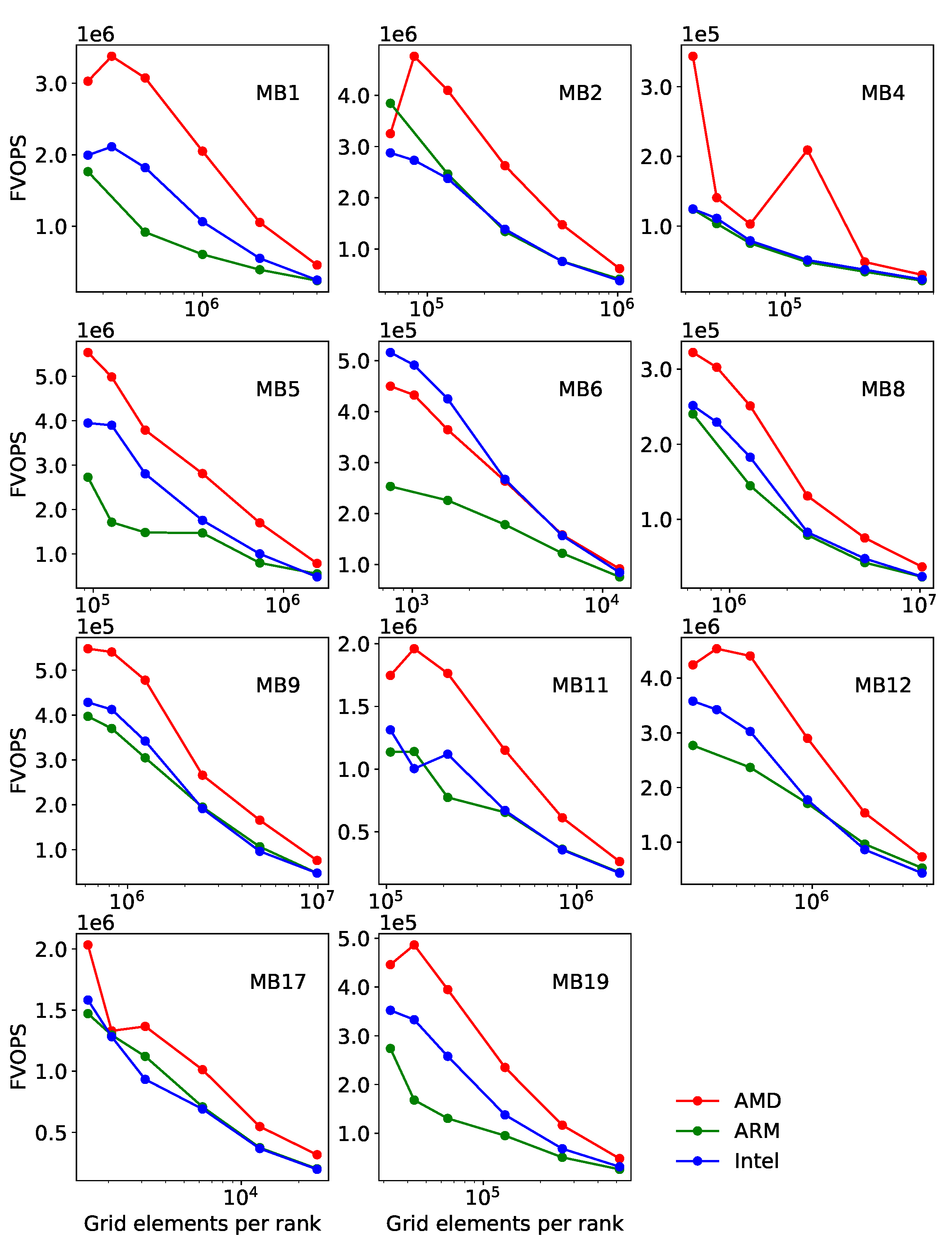
Figure 16.
Box plots of the FVOPS metric with all grid sizes for different microbenchmarks.
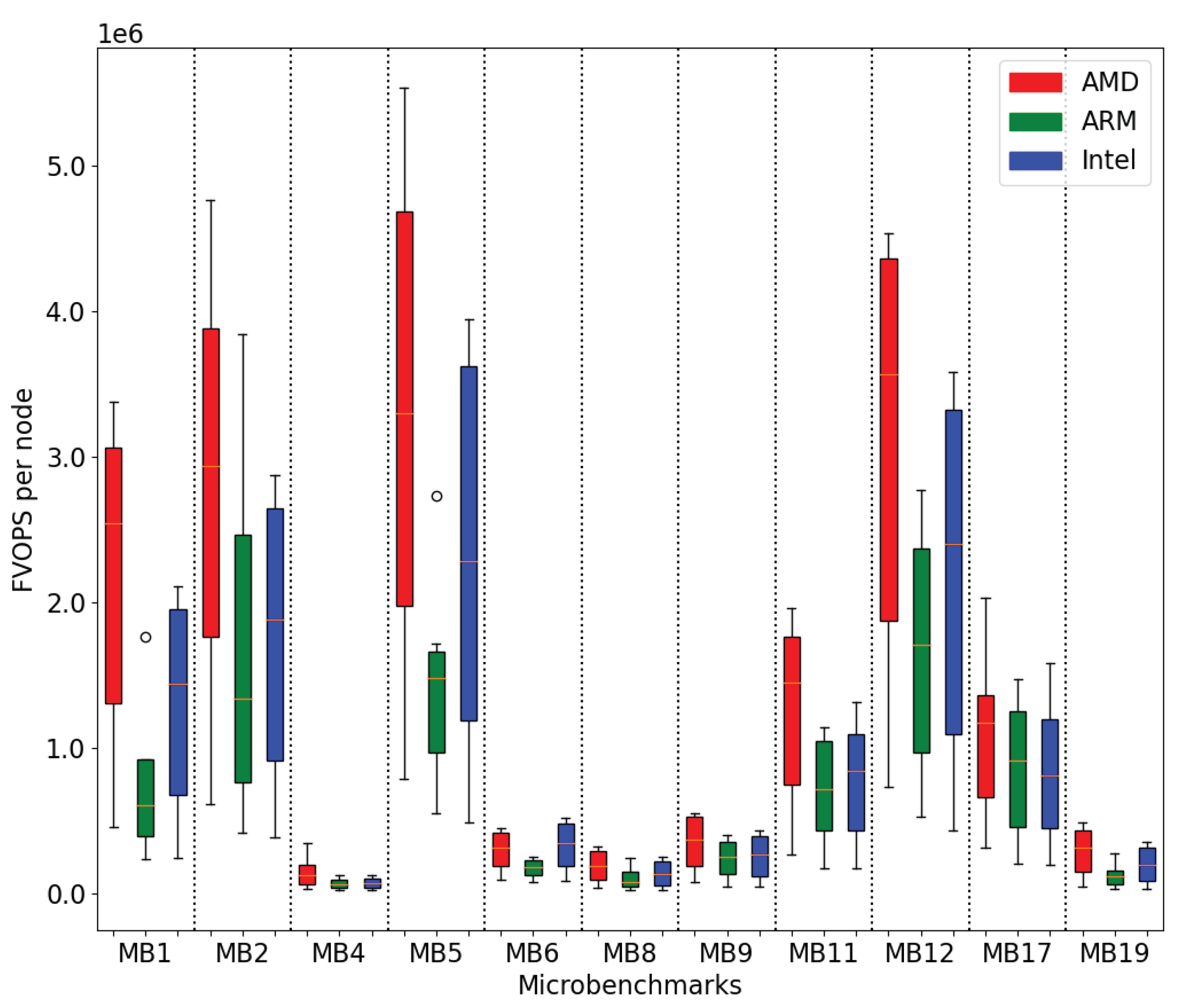

Table 1.
Summary of the architectures and processor types utilized for the tests.
| Architecture | CPU Model | Frequency | Cores/node | Memory/node |
|---|---|---|---|---|
| x86_64 | Intel(R) Xeon(R) Gold 6226R (Cascade Lake) | 2.9 GHz | 32 | 192 GB |
| x86_64 | AMD EPYC 7313 16-Core Processor (Milan) | 3.3 GHz | 32 | 256 GB |
| aarch64 | Arm Neoverse-N1 | 3.0 GHz | 256 | 512 GB |
Table 2.
Summary of the OpenFOAM MBs considered in this study. Mesh generation types are blockMesh (BM), snappyHexMesh (SHM) and cfMesh (CFM).
Table 2.
Summary of the OpenFOAM MBs considered in this study. Mesh generation types are blockMesh (BM), snappyHexMesh (SHM) and cfMesh (CFM).
| Microbenchmarks | Top-Level Solver | Mesh generation - Cell count - Cell type |
|---|---|---|
| MB1 Cavity 3D | icoFoam | BM - 8M - Hexahedra |
| MB2 Compressible starting square jet | rhoPimpleFoam | BM - 2M - Hexahedra |
| MB4 DLR-JHC burner | reactingFoam | BM - 400k - Hexahedra |
| MB5 ERCOFTAC Conical diffuser | simpleFoam | BM - 3M - Hexahedra |
| MB6 Two cylinders in line | adjointOptimisationFoam | BM - 24500 - Hexahedra |
| MB8 Rotating Wheel | pimpleFoam | SHM - 20M - Polyhedra |
| MB9 High-lift airfoil | rhoPimpleFoam | SHM - 20M - Polyhedra |
| MB11 Pitz&Daily Combustor | XiFoam | BM - 200k - Hexahedra |
| MB12 Model Wind Farm | pimpleFoam | BM - 8M - Hexahedra |
| MB17 1D Aeroacoustic Wave Train | rhoPimpleFoam 1D | BM - 0.05M - Hexahedra |
| MB19 Viscoelastic polymer melt flow | viscoelasticFluidFoam | CFM - 1M -Polyhedra |
Disclaimer/Publisher’s Note: The statements, opinions and data contained in all publications are solely those of the individual author(s) and contributor(s) and not of MDPI and/or the editor(s). MDPI and/or the editor(s) disclaim responsibility for any injury to people or property resulting from any ideas, methods, instructions or products referred to in the content. |
© 2024 by the authors. Licensee MDPI, Basel, Switzerland. This article is an open access article distributed under the terms and conditions of the Creative Commons Attribution (CC BY) license (http://creativecommons.org/licenses/by/4.0/).
Copyright: This open access article is published under a Creative Commons CC BY 4.0 license, which permit the free download, distribution, and reuse, provided that the author and preprint are cited in any reuse.


