Submitted:
03 March 2024
Posted:
05 March 2024
You are already at the latest version
Abstract
Classical Arabic poetry is a form of Arabic literature, and almost every piece of Arabic poetry follows one of the 16 meters. The rhythmic framework of the poems or the verses is called meters. The deep learning (DL) model was implemented using TensorFlow in this work using a large dataset of Arabic poetry. The character level encoding was used to convert text to integers for classifying the full-verse and half-verse data. The study evaluates the data without removing diacritics from the text. The train-test-split method with a 70-15-15 split was employed for classification. 15% of the total data was considered unseen test data for all models. The work was conducted with multiple deep learning models, including the Long Short-Term Memory (LSTM), Gated Recurrent Units (GRU), and Bidirectional LSTM (Bi-LSTM). The Bi-LSTM model shows the best accuracy of all the models specified, with 97.53% for full-verse and 95.23% for half-verse without removing diacritic data.
Keywords:
Arabic poetry
; Arabic meters
; Bi-LSTM
; Deep learning
; Machine learning
; Natural language processing
1. Introduction
Arabic prosody (Arud) has been studied for many years in morphology and phonetics. The study of meters in poetry enables us to determine whether the poetry is sound or broken [1]. Some of the terminology used most frequently in Arabic prosody are as follows: the poetry’s single line comprises two verses, each half verse called a "bayt." The first verse is "sadder," and the second is "ajuz." Classical Arabic poetry, defined by units called Meters, was analyzed by the famous lexicographer and grammarian Al-Khalil ibn Ahmad al-Farahidi in the 8th century [2]. The meter is based on the syllables part of a word and has two parts: short and long syllables. The sixteen meters are Tawiil, Basiit, Madid, Waafir, Kaamil, Hazaj, Rajaz, Ramal, Munsarih, Khafiif, Muqtadab, Mujtath, Mudaari', Sarii', Mutaqaarib and Mutadaarik. The ode may consist of 120 lines, split into two half-lines characterized by their meter, repeated for the whole verse. Al-Farahidi represented some feet provided in a rhythmic to make it easy to remember the meter (fa'uulun, mafaa'iilun).
Poetry is a way of communication, interaction, and an essential aspect of any language and literature. Communities, nations, and societies have expressed themselves through poetry for ages. Poetry is hard to understand since it has a specific pattern and underlying meanings in its words and phrases, making it different from prose. It is necessary to understand the structure to understand the poetry completely. Bahar is the meters in Arud science. Arud science helps to divide Arabic poems into 16 meters, making them easy to understand without referring to the context (Alnagdawi et al., 2013). Classical Arabic poetry can be recognized and understood using various methods and tools. Arud is the rule and regulations of poems used in many languages (Abuata & Al-Omari, 2018). Poetry is different from prose mainly because of its form and structure. Poetry consists of tone, metrical forms, rhythm, imagery, and symbolism. In Arabic poetry, each line ends with a specific tone. The field that studies rhyme and rhythm is called prosody and is complex due to many overlapping rules (Khalaf et al., 2009).
There are two vowels in modern and classical Arabic: long and short. The long vowels are explicitly written, and short vowels are also called diacritic. Various attempts have been carried out to implement Arabic text. A proposal was made to use Arabic diacritics or 'harakat' for text hiding for security purposes (Ahmadoh & Gutub, 2015). The diacritics in Arabic are split into three parts, as shown in Table 1. Most works in this field use a deep learning method to diacritized the Arabic text before loading it into the model [3,4].
Artificial Intelligence (AI) has become exponentially more practical and significant over the last few years. The AI-enabled state-of-the-art technologies have expanded substantially and shown effective results in almost every industry, such as security [5], surveillance, health [6], automobiles [7], fitness tracking [8] and smart homes [9], etc. In general, AI and machine learning (ML) are correlated. They are primarily used to develop intelligent systems [10]. Deep Learning (DL) is a type of ML that allows computers to learn from data representation with more neural levels. Convolutional neural networks (CNN) have revolutionized image, video, and audio processing, and Recurrent neural networks (RNN) have gained insight into text and speech sequential data [11]. Any deep learning model's design must consider the choice of algorithm. Most sequential applications follow the RNN model [12], and it has the context of previous input but not the future context of the speech or text data. Bidirectional recurrent neural networks (Bi-RNN) extract the data's context in both forward and backward directions [13].
This study employed Arabic text without removing diacritics from the poetry dataset. We considered 14 meters and removed two meters with very little data compared to other meters. The RNN models like GRU and LSTM and Bi-RNN models like Bi-LSTM are used to implement the proposed work. We achieved better performance than previous studies on full-verse and half-verse meter classification. The research question for this study is as follows:
RQ: How does the choice of the number of hidden layers impact the performance of the Arabic meter classification model using DL models?
The remaining section of this paper is organized into six sections. The literature review, including Arabic meter and DL models, is explained in section two. Section three describes the methodology used and the model algorithm. The results are presented in detail in section four, with a discussion in section five. The conclusion with future work is described in section six.
2. Literature Review
Alnagdawi [2] used Another Tool for Language Recognition to find the meter of Arabic poems. This tool works in three steps: first, it converts poetry into Arud form. The second step is the segmentation of the Arud form. In this phase, the Arud state is divided into sounds, such as short sounds, vowel or long sounds, and consonants. The sound string was sent to the final stage at the end of the second step, and the poetry meter was detected. It is compared with grammar to check its validity. If the grammar is valid, the verse belongs to sixteen meters. The meter patterns match the poem's words, identifying the meter's name.
A considerable body of literature is on recognizing Arabic poetry using deep learning algorithms. Baina and Moutassaref [14] developed an algorithm that accurately identifies the poem's meter and outputs the 'Arud' writing in addition to the meter. The algorithm follows five phases. First, it adds diacritics to the verse. This step is significant as it might impede moving to the next step. Second, it transforms the diacritics into 'Arud' writing. Third, it utilizes binary representation to convert the 'Arud' writing, where 1 represents a 'haraka,' and 0 illustrates a 'sukon.' Fourth, the algorithm identifies the meter based on the binary representation. The fifth and final step includes detecting the errors and ensuring the meter matches the poem.
Furthermore, [15] proposed a narrow, deep neural network with significantly high accuracy. The proposed network consists of an embedding layer at its input, BiLSTM layers that counted to be five, a concentration layer, and an output layer provided with softmax activation. Similarly, [4] suggested improving the recognition of diacritics via a specific neural network. This strategy tries to enhance readability and recognition accuracy. Moreover, identifying the meter of an Arabic poem may be a long and complicated process that involves a few steps [16]. A study by [17] utilizes machine learning algorithms to identify and classify Arabic texts. The study supports linear vector classification and naïve Bayes classification, which have the highest precision. Many studies have been conducted on analyzing Arabic poetry. Formulating one system or technique to identify meters in Arabic poetry is challenging. A study on identifying Arabic poetic meter [18] suggested a method that produces coded Al-Khalyli transcriptions of Arabic.
Abuata and Asama Al-Omari [19] electronically analyze the Arud meter of Arabic poetry. They introduce an algorithm to determine the meter of Arud for any Arabic poetry. The algorithm works on well-defined rules applied only to the first part of the poem verse. Moreover, some of the most outstanding works in Arabic poetry are the computerization of Arabic poetry meters [20]. It focuses on computerizing El- Katib's method for analyzing Arabic poetry. The linguist El-katib proposed a study in which poetry is converted into binary bits and given decimal codes. This system was helpful for educational purposes. Many students and teachers use it to understand prosody. The computerized and systematic analysis of prosody also minimizes the chance of error.
Attempts have been made to develop Algorithms that recognize modern Arabic poetry meters [3,4,16]. For instance, an algorithm has been introduced to identify standard features of classical Arabic poems [21]. These features include rhyme, rhythm, punctuation, and text alignment. This algorithm can only recognize whether the Arabic piece is poetic or non-poetic but cannot acknowledge its meter. Furthermore, an algorithm has been developed to detect the Arabic meter of certain poetry and convert the verse into 'Arud' writing [22]. It uses meters or 'Bahr' to classify Arabic poetry. It investigates the methods of detecting Arabic poems in rhythm, rhyme, and meter. It utilizes time and non-time series representation of the MFCC (Mel Frequency Cepstral Coefficients) and LPCC (Linear Predictive Cepstral Coefficients) features to recognize automated 'Arud' meters. Arabic 'Arud' meters seem to possess a time-series nature; however, the non-time series representation performs better.
Another detection method includes a comparison that has been conducted between modern and classical Arabic poetry [23]. Results reveal that contemporary Arabic poetry lacks more distinctive features than classical poetry. For instance, modern Arabic poetry is characterized by partial meter, the uneven lining of verses, word repetition, usage of punctuation, and irregular rhyming. At the same time, classical Arabic poetry is characterized by a regular rhyme, a single meter, even lining of verses, and self-contained lines. Similarly, [24] assert that extracting the poem's meter using automatic meter detection methods requires challenging data collection and processing efforts. Syllable segmentation and similarity checks are performed. This method has further proven the high accuracy of meter detection. Finally, creating detecting algorithms may considerably improve the efficiency and accuracy of Arabic poetry identification methods.
The LSTM model is one of the most widely used RNN systems for vanishing gradients [25]. In addition, these networks have several advantages compared to conventional RNN systems, including the ability to sustain prolonged interrelationships and exhibit stochastic nature when dealing with time-series input data. With RNN or LSTM, the uniform weight is retained across all layers, limiting the number of parameters the network must learn. There were more parameters in LSTM, which made it slower.
Later, GRUs were proposed as a better alternative to LSTMs and have gained significant recognition [26]. In addition, GRUs have been recognized to be effective in numerous applications using sequential or time-series input [27]. For instance, they have been incorporated in diverse areas such as speech synthesis, NLP, and signal processing. Furthermore, LSTM, RNNs, and GRUs have been exhibited to operate better in long-sequence applications. In GRUs, gating network signaling plays a significant role since it controls how inputs and memory are used to update current activations. Each gate has weights that are adapted and modified in the learning phase. However, these systems enable effective learning in RNNs, increasing parameterization. It leads to a simpler RNN model with a higher computational cost. The LSTM and GRU differ because the former utilize three novel gate networks, whereas the latter uses only 2.
The Bi-LSTM neural network comprises LSTM units that operate in both directions to exploit contextual information from the past and future [28]. In addition, with Bi-LSTM, long-term dependencies can be learned without maintaining redundant background information. Thus, it has projected significant performance for sequential modeling issues and is generally used for text classification [29]. Bi-LSTM networks transmit forward and reverse phases in both directions, unlike LSTM networks, which communicate only in one direction.
3. Materials and Method
Neural networks were the foundation for the classification model that was used. DL is preferred because the data size has a large amount of volume. The experiment is conducted using the guidelines outlined in Table 2.
The methodology of the work is shown in Figure 1. Fetching the data set, preprocessing, and splitting the data, and developing and applying the DL models are the key phases of the work. A combination of accuracy, precision, recall, and the F1_score was used to evaluate the results.
3.1. Dataset and Preprocessing
The dataset contains 1,862,046 verses with 22 meters [37]. The data is in a well-structured format. The central 16 meters consists of a data size of 1,647,854. Two meters with fewer verses are avoided when classifying the meters. After eliminating the empty cells, the total number of verses in the 14 meters of data, which include both right and left verses, is 1,646,771. The count of each meter label with a full-verse is depicted in Figure 2. The minimum count is for the Mutadarik meter, 4507 verses, and the maximum is for the Tawil meter, 398239 verses. Half-verse data is doubled for training since each meter's left and right verses are considered separate.
The datasets are cleaned by removing symbols and other non-Arabic characters. The methodology of [16] is followed here. The vocabulary is created according to the characters in the dataset, and each character is labeled an index value. Character level encoding uses the index value for each cleaned text and uses DL models for implementation. The parameters are tuned for each model. The data is split into 70% training and 15% validation; the remaining 15% is set as unseen data for testing.
3.2. Deep Learning Models
This study uses the deep neural network (DNN) architecture. The two main architectures of DNN are RNN and CNN [31]. LSTM, GRU, Bi-LSTM are models under RNN [38]. The base model for LSTM is shown in Figure 3 (a). The first layer of the sequential model is the input layer with the size of the padded sequence, which is then given to the embedding layer with the output dimension kept as 64. The embedding layer will learn the mapping of the characters to vectors. The output from the embedding layer is fed into the LSTM layer with units 256, recurrent, and the activation function is set as the default. The LSTM layer is added accordingly to increase the hidden layers. At this moment, the return sequence parameter should be set as 'True.' The GRU model, Figure 3 (b), is like the LSTM model. In both models, sentence processing is only in one direction.
The LSTM layer is depicted in Figure 4. It allows the model to store the information for future access and has a hidden state: short-term memory. There are three gates for LSTM such as input (it), output (Ot), and forget gate (ft). A time step is indicated by the subscript 't.' The LSTM has three inputs: an input vector at the current time stamp (Xt), a cell or memory state vector (Ct-1), and a hidden state vector at the previous time stamp (ht-1). The symbol '×' denotes the element-wise product or the Hadamard product. is the cell state activation vector or the candidate memory vector [39].
As a first step, determine what information the cell state should discard. It is accomplished by the sigmoid activation function (σ) in the forget gate and applies the sigmoid function to the current input vector Xt and the past hidden state vector ht-1. Input activations activate memory cells through input gates.
where ft = forget gate, wf, and uf are the forget gate's weight matrix, Xt is the actual input, bf is the bias vector, and ht-1 is the hidden state output from the previous time stamp. The result from Eq 1 is in the range of 0 and 1. The element-wise product of Ct-1 and ft decides what information to retain and forget.
The second step is to update the memory cell with an input gate. The sigmoid function indicates two values; if it is one, the actual data is unchanged, and if it is zero, it will be dropped. A tanh function is applied to the selected input values, which indicates a range from -1 to +1. It creates a new vector of values, a candidate memory cell.
where it = input gate, wi, and ui are the input gate's weight matrix, and bi is the bias vector.
where = candidate memory cell, wc, and uc are the weight matrix, and bc is the bias vector.
The following step involves updating and converting the previous cell state Ct-1 to the new Ct. The equation is defined as
where ft = forget gate calculated from Eq 1, Ct-1 is the memory state vector of the previous time stamp, it = input gate calculated from Eq 2, and is candidate memory cell from Eq 3.
The final stage is to decide what portion of the output will be selected. It is done in two steps. First, the sigmoid function is performed with the input to determine the quantity of cell state to transmit as the output. The tanh operation is then applied to the new cell state Ct, and the sigmoid result is multiplied by the result. Thus, the outcome is based only on the selected portions.
where Ot = output gate, wo, and uo are the output gate's weight matrix, and bo is the bias vector.
where Ot = output gate calculated from Eq 5, and new cell state Ct calculated from Eq 4.
The GRU layer is illustrated in Figure 5. A reset gate and an update gate are two gates. But the GRU requires fewer parameters to train than the LSTM model, which runs faster. The reset gate (Rt) regulates the amount of the initial state that needs to be remembered. Similarly, an update gate (Zt) enables us to assess how much the new form replicates the previous one. As each hidden unit reads/generates a sequence, these two gates control how much of it is remembered or forgotten [39].
The reset gate performs similar functions to LSTM's forgotten gate. It manages a network's short-term memory. A decision is made regarding what information should be forgotten.
where Rt = reset gate, wr, and ur are the reset gate's weight matrix, br is the bias vector, Xt is the actual input, and ht-1 is the hidden state output from the previous time stamp.
The update gate manages the network's long-term memory. It accomplishes a similar task as the forget and input gate of an LSTM. It determines what data should be removed and what new data should be added.
where Zt = update gate, wz, and uz are the update gate's weight matrix, and bz is the bias vector.
The candidate's hidden state () is also called an intermediate memory unit, which combines the previously hidden state vector in the reset gate with the input vector.
where = candidate hidden state vector, wh, and uh are the weight matrix, bh is the bias vector, and Rt = reset gate calculated from Eq 7.
The final hidden state is determined based on the update gate and candidate hidden state. The update gate is multiplied element-wise and summed with the candidate vector.
where ht is the hidden state output, Zt = update gate calculated from Eq 8, and = candidate hidden state vector calculated from Eq 9.
The BiLSTM model processes the sequence in both directions of a text. One hidden layer is in the forward movement, and the other is backward. These LSTM layers are concatenated for the final output of the BiLSTM layer. So, unit 256 is doubled in this model. LSTM's return sequence parameter is set to 'True' if two or more layers need to be added. The baseline model for BiLSTM is shown in Figure 6. The Dropout parameter in the BiLSTM layer is set to 0.2, which helps to prevent the training model from overfitting. The hidden layers are tuned from 1 to 3 in all three models.
A better iteration of LSTM is the BiLSTM layer, which processes the sequence in forwarding and backward directions, as shown in Figure 7. The BiLSTM can understand the context better than the LSTM and GRU models [40]. It contains the LSTM model architecture as described in Figure 4. Xt and Xt+1 are the input vectors at time frame t.
While calculating the forward output sequence (), the positive sequence is used, and when calculating the backward output sequence, (), the reverse inputs are used. The output vector, yt, is obtained by combining the forward and backward output sequences.
where is the forward output sequence, is the backward output sequence. The symbol 'ʃ' can have different operations such as summation, multiplication, concatenation, and average function. The default function in TensorFlow is concatenation.
The optimizer used for the compilation is adaptive moment estimation (Adam). This memory-light optimization algorithm works well with large datasets [41]. Since the method label_encoder provides a sparse array of targets, the loss function uses a sparse_categorical cross-entropy.
3.2.1. Hyper-Parameter Tuning
The tuned parameters are the hidden layer and learning rate for the above models. The hidden layers are tuned from one to three in all the 3 DL models. EarlyStopping is used in the TensorFlow model's callback application programming interface (API) to stop overfitting the models. In this, the parameter 'patience' is set to 6, so the training will terminate if the validation loss function does not decrease after six epochs. Another function used is ReduceLROnPlateau. This function's monitoring parameter is set to validity loss, patience is 3, and the minimum learning rate is 1.0*10-6. It indicates that if the loss value does not change after two epochs, the learning rate value decreases by 0.1. So, the new rate for the next epoch will be 0.1 times the previous rate. The most accurate model is chosen based on the accuracy of the validation set, and it is then applied to the test set.
3.3. Evaluation Metrics
Accuracy, precision, recall, and f1-score are the metrics used to assess the classification model on the test data. For each technique, the confusion matrix is also considered. Accuracy might not be a complete metric for unbalanced data [42]. So precision, recall, and f1-score are also used [43,44]. Accuracy is the total sample count that was successfully predicted. Precision determines how many predicted samples are relevant. Recall computes how many relevant samples are predicted. Calculating the harmonic mean of recall and precision yields an f1-score.
Precision is also called a positive predictive rate (PPR), and recall is known as Sensitivity. Three performance measures are calculated using the following formulas.
where TruePose is a true positive, TrueNega is a true negative, FalsePose is a false positive, and FalseNega is a false negative. When the model correctly predicted the positive label, the result was considered TruePose. Similarly, if the model predicts a negative label correctly, the outcome is TrueNega. On the other hand, FalsePose is calculated based on the incorrectly predicted positive label, and FalseNega is based on the incorrectly predicted negative label.
4. Results
This paper considers the classification of Arabic meters using three DL methods. The GPU was used for running the model. These models were developed using the Python language and Tensorflow DL libraries [45]. The diacritics are not removed for both the full and half-verse data.
4.1. Training and Testing Using Full-Verse
The full-verse data is split according to 70% for training, 15% for validation, and 15% for testing. The validation accuracy according to the hidden layers is tabulated in Table 3 for the full-verse data. Also, the number of parameters the model uses for training is specified (in millions). The trainable parameter also increases; hence, the time taken to complete the execution also increases. The training epochs are set to 60 for all the models. Callback applications like EarlyStopping and ReduceLROnPlateau evaluate whether the model overfits. The validation loss is the parameter to check in the ReduceLROnPlateau function. If the loss value is found stable for three epochs, then the learning parameter is increased. For the EarlyStopping function, the program stops where it finds the loss value increases from the previous value or is stable for around six epochs. The training epochs in Table 3 show the number of epochs each model took without overfitting the data. The LSTM, GRU, and BiLSTM models perform better at three layers. And compared to the three models, the BiLSTM shows an accuracy of 97.53%.
The training and validation loss and accuracy of the BiLSTM with three layers are depicted in Figure 8. The training loss indicates how well a DL model fits the training set. Validation loss measures the performance of the validation set. Accuracy increases as the loss value decreases.
The confusion matrix of the BiLSTM 3-layer model is shown in Figure 9. The model was tested with the remaining 15% of unseen data. All the labels show good model fitting, and there was no overfitting or underfitting problem with the model performance.
The complete details of the model performance are depicted in Table 4. Each meter or label's precision, recall, accuracy, and f1-score are evaluated. The basit and tawil meters show the highest accuracy of 99%. The low performance is demonstrated by the hazaj meter with 80% accuracy.
4.2. Training and Testing Using Half-Verse
The study also implemented the model based on the half-verse data without removing diacritics. The half-verse data count is double the number of full-verse data, and the data is split into 70% training, 15% validation, and 15% testing. The hidden layers are tuned from one to three, as shown in Table 5. Increasing the layers increases the parameters to train the model. Also, the time to complete the training increases according to hidden layers. Even though the BiLSTM model exists in 31 epochs, it took approximately 11 hours to complete the execution.
The best model is BiLSTM, with 95.23% accuracy. The training and validation accuracy and loss values are depicted in Figure 10. Both the loss and accuracy are inversely proportional to each other. The model exits from the iteration if the loss value is stable for six epochs.
The confusion matrix and the complete details of the target meters results are shown in Figure 11 and Table 6, respectively.
The model shows better performance, as seen in Table 6. The highest-class accuracy is demonstrated by basit and tawil meter with 98% accuracy. The lowest performance is shown by the hazaj meter, which has 74% accuracy.
5. Discussions
The BiLSTM model predicts the data better when compared with LSTM and GRU. This model's sequence learning is in both directions, from left to right and right to left. GRU trains faster than LSTM, with fewer training parameters than LSTM [46]. Few works are done on Arabic poetry, including the diacritization of the text data. The work of [3] shows a BiLSTM model with automatic diacritization. The results show a 42% improvement in the error rate of diacritization. The study of [36] was based on machine learning algorithms and a diacritic text. An accuracy of 96.34% was achieved using support vector machines (SVM).
The proposed work can be compared with the studies of [4,16]. With five hidden layers, [16] study reached an accuracy of 94.32% with the bi-directional GRU (BiGRU) model and 14 target meters. The model also attains 88.8% accuracy for half-verse data. With four hidden layers, the BiLSTM model of [4] study achieved an accuracy of 97% without removing diacritics and 97.27% with removed diacritics. They use 16 meters as target classes. The work done by [37] uses seven hidden layers for the BiLSTM model and achieved an accuracy of 96.38%. In our proposed research, the number of verses is much higher than in the study done by [16]. Also, the number of hidden layers is less than in all three studies. The comparison of Arabic meter studies is mentioned in Table 7.
In the proposed study, the BiLSTM model with three hidden layers performs better than one or two hidden layers without removing diacritical text. Also, it better predicts than the LSTM and GRU models for both full-verse and half-verse data. LSTM cannot use future tokens, nor can local contextual information be extracted. This problem can be resolved using BiLSTM, which learns the sequence in forward and backward directions. GRUs are faster to train than the LSTM model but lack the output gate. We achieved an accuracy of 97.53% for the full-verse data and 95.23% for the half-verse data.
The study's results suggest that the number of hidden layers significantly impacts the performance of the Arabic meter classification model using Bi-LSTM. Our study achieved better accuracy in Arabic meter classification using Bi-LSTM models with three hidden layers compared to previous studies that used Bi-LSTM models with 4 and 7 hidden layers. It suggests that increasing the number of hidden layers beyond a certain point may not always lead to better performance and that optimizing the number of hidden layers can be a crucial factor in achieving high accuracy.
6. Conclusion
For many years, morphology and phonetics have studied Arabic prosody. Prosody is the study of meters in poetry, determining whether the poem's lines have a sound or a broken meter. The phonetic location of stress in Arabic has been investigated. On the other hand, pressure could be a cognitive phenomenon involving linguistic rhythm manifested in various physical forms. Since the data is enormous, this study predicts 14 Arabic meters with different DL models. The diacritics are not removed from the text and are used for classifying the meters. The BiLSTM model shows higher accuracy with three hidden layers. The model achieved 97.53% accuracy and 95.23% for full-verse and half-verse data, respectively. The detection of Arabic meters will continue to be a focus of our future work, which includes balancing the data, diacritizing Arabic text, and integrating deep learning models into the existing model.
Author Contributions
Conceptualization, methodology, supervision, and writing—review and editing, A.M.; data acquisition, methodology, experiment, and writing— original draft preparation, AA. All authors read and approved the submitted version of the manuscript.
Funding
This research received no external funding.
Data Availability Statement
The data presented in this study are openly available [37].
Conflicts of Interest
The authors declare no conflicts of interest.
References
- Jones, A. Early Arabic Poetry: Select Poems. Available online: https://api.pageplace.de/preview/DT0400.9780863725555_A25858721/preview-9780863725555_A25858721.pdf (accessed on 9 September 2022).
- Alnagdawi, M.; Rashaideh, H.; Aburumman, A. Finding Arabic Poem Meter using Context Free Grammar. Journal of Communications and Computer Engineering 2013, 3, 52–59. [Google Scholar] [CrossRef]
- Abandah, G.A.; Suyyagh, A.E.; Abdel-Majeed, M.R. Transfer learning and multi-phase training for accurate diacritization of Arabic poetry. Journal of King Saud University-Computer and Information Sciences 2022, 34, 3744–3757. [Google Scholar] [CrossRef]
- Abandah, G.A.; Khedher, M.Z.; Abdel-Majeed, M.R.; Mansour, H.M.; Hulliel, S.F.; Bisharat, L.M. Classifying and diacritizing Arabic poems using deep recurrent neural networks. Journal of King Saud University-Computer and Information Sciences 2020, 34, 3775–3788. [Google Scholar] [CrossRef]
- Wu, H.; Han, H.; Wang, X.; Sun, S. Research on artificial intelligence enhancing internet of things security: A survey. IEEE Access 2020, 8, 153826–153848. [Google Scholar] [CrossRef]
- Davenport, T.; Kalakota, R. The potential for artificial intelligence in healthcare. Future healthcare journal 2019, 6, 94. [Google Scholar] [CrossRef] [PubMed]
- Manoharan, S. An improved safety algorithm for artificial intelligence enabled processors in self driving cars. Journal of artificial intelligence 2019, 1, 95–104. [Google Scholar]
- Fietkiewicz, K.; Ilhan, A. Fitness tracking technologies: Data privacy doesn’t matter? The (un) concerns of users, former users, and non-users. Proceedings of the 53rd Hawaii International Conference on System Sciences 2020. [Google Scholar] [CrossRef]
- Gochoo, M.; Tahir, S.B.U.D.; Jalal, A.; Kim, K. Monitoring Real-time Personal Locomotion Behaviors over Smart Indoor-outdoor Environments via Body-Worn Sensors. IEEE Access 2021, 9, 70556–70570. [Google Scholar] [CrossRef]
- Das, S.; Dey, A.; Pal, A.; Roy, N. Applications of artificial intelligence in machine learning: review and prospect. International Journal of Computer Applications 2015, 115, 31–41. [Google Scholar] [CrossRef]
- LeCun, Y.; Bengio, Y.; Hinton, G. Deep learning. nature 2015, 521, 436–444. [Google Scholar] [CrossRef]
- Iqbal, T.; Qureshi, S. The survey: Text generation models in deep learning. Journal of King Saud University - Computer and Information Sciences 2022, 34, 2515–2528. [Google Scholar] [CrossRef]
- Schuster, M.; Paliwal, K.K. Bidirectional recurrent neural networks. IEEE transactions on Signal Processing 1997, 45, 2673–2681. [Google Scholar] [CrossRef]
- Baïna, K.; Moutassaref, H. An Efficient Lightweight Algorithm for Automatic Meters Identification and Error Management in Arabic Poetry. Proceedings of the 13th International Conference on Intelligent Systems: Theories and Applications 2020, 1–6. [Google Scholar] [CrossRef]
- Albaddawi, M.M.; Abandah, G.A. Pattern and Poet Recognition of Arabic Poems Using BiLSTM Networks. 2021 IEEE Jordan International Joint Conference on Electrical Engineering and Information Technology (JEEIT) 2021, 72–77. [Google Scholar] [CrossRef]
- Al-shaibani, M.S.; Alyafeai, Z.; Ahmad, I. Meter classification of Arabic poems using deep bidirectional recurrent neural networks. Pattern Recognition Letters 2020, 136, 1–7. [Google Scholar] [CrossRef]
- Ahmed, M.A.; Hasan, R.A.; Ali, A.H.; Mohammed, M.A. The classification of the modern arabic poetry using machine learning. Telkomnika 2019, 17, 2667–2674. [Google Scholar] [CrossRef]
- Saleh, A.-Z.A.K.; Elshafei, M. Arabic poetry meter identification system and method. US Patent US Patent No. 8,219,386, 2012. [Google Scholar]
- Abuata, B.; Al-Omari, A. A rule-based algorithm for the detection of arud meter in CLASSICAL Arabic poetry. International Arab Journal of Information Technology 2018, 15, 1–5. [Google Scholar]
- Khalaf, Z.; Alabbas, M.; Ali, S. Computerization of Arabic poetry meters. UOS Journal of Pure & Applied Science 2009, 6, 41–62. [Google Scholar]
- Zeyada, S.; Eladawy, M.; Ismail, M.; Keshk, H. A Proposed System for the Identification of Modem Arabic Poetry Meters (IMAP). 2020 15th International Conference on Computer Engineering and Systems (ICCES) 2020, 1–5. [Google Scholar] [CrossRef]
- Al-Talabani, A.K. Automatic recognition of Arabic poetry meter from speech signal using long short-term memory and support vector machine. ARO-The Scientific Journal of Koya University 2020, 8, 50–54. [Google Scholar] [CrossRef]
- Almuhareb, A.; Almutairi, W.A.; Al-Tuwaijri, H.; Almubarak, A.; Khan, M. Recognition of Modern Arabic Poems. Journal of Software. 2015, 10, 454–464. [Google Scholar] [CrossRef]
- Berkani, A.; Holzer, A.; Stoffel, K. Pattern matching in meter detection of Arabic classical poetry. 2020 IEEE/ACS 17th International Conference on Computer Systems and Applications (AICCSA) 2020, -8, 1–8. [Google Scholar] [CrossRef]
- Hochreiter, S.; Schmidhuber, J. Long short-term memory. Neural computation 1997, 9, 1735–1780. [Google Scholar] [CrossRef]
- Cho, K.; Van Merriënboer, B.; Gulcehre, C.; Bahdanau, D.; Bougares, F.; Schwenk, H.; Bengio, Y. Learning phrase representations using RNN encoder-decoder for statistical machine translation. Proceedings of the 2014 Conference on Empirical Methods in Natural Language Processing (EMNLP) 2014, 1724–1734. [Google Scholar]
- Dey, R.; Salem, F.M. Gate-variants of gated recurrent unit (GRU) neural networks. 2017 IEEE 60th international midwest symposium on circuits and systems (MWSCAS) 2017, 1597–1600. [Google Scholar] [CrossRef]
- Liang, D.; Zhang, Y. AC-BLSTM: asymmetric convolutional bidirectional LSTM networks for text classification. arXiv preprint 2016, arXiv:1611.01884. [Google Scholar]
- Huang, Z.; Xu, W.; Yu, K. Bidirectional LSTM-CRF models for sequence tagging. arXiv preprint 2015, arXiv:1508.01991 2015. [Google Scholar]
- Wazery, Y.M.; Saleh, M.E.; Alharbi, A.; Ali, A.A. Abstractive Arabic Text Summarization Based on Deep Learning. Computational Intelligence and Neuroscience 2022, 2022. [Google Scholar] [CrossRef]
- Yin, W.; Kann, K.; Yu, M.; Schütze, H. Comparative study of CNN and RNN for natural language processing. arXiv preprint 2017, arXiv:1702.01923 2017. [Google Scholar]
- Huang, Z.; Xu, W.; Yu, K. Bidirectional LSTM-CRF models for sequence tagging. arXiv preprint 2015, arXiv:1508.01991. [Google Scholar] [CrossRef]
- El Rifai, H.; Al Qadi, L.; Elnagar, A. Arabic text classification: the need for multi-labeling systems. Neural Computing and Applications 2022, 34, 1135–1159. [Google Scholar] [CrossRef]
- Chen, H.; Wu, L.; Chen, J.; Lu, W.; Ding, J. A comparative study of automated legal text classification using random forests and deep learning. Information Processing & Management 2022, 59, 102798. [Google Scholar] [CrossRef]
- Abdulghani, F.A.; Abdullah, N.A. A Survey on Arabic Text Classification Using Deep and Machine Learning Algorithms. Iraqi Journal of Science 2022, 409–419. [Google Scholar] [CrossRef]
- Alqasemi, F.; Salah, A.-H.; Abdu, N.A.A.; Al-Helali, B.; Al-Gaphari, G. Arabic Poetry Meter Categorization Using Machine Learning Based on Customized Feature Extraction. 2021 International Conference on Intelligent Technology, System and Service for Internet of Everything (ITSS-IoE) 2021, -4, 1–4. [Google Scholar] [CrossRef]
- Yousef, W.A.; Ibrahime, O.M.; Madbouly, T.M.; Mahmoud, M.A. Learning meters of Arabic and English poems with Recurrent Neural Networks: a step forward for language understanding and synthesis. arXiv preprint 2019, arXiv:1905.05700 2019. [Google Scholar]
- Sherstinsky, A. Fundamentals of recurrent neural network (RNN) and long short-term memory (LSTM) network. Physica D: Nonlinear Phenomena 2020, 404, 132306. [Google Scholar] [CrossRef]
- Harrou, F.; Sun, Y.; Hering, A.S.; Madakyaru, M.; Dairi, A. Chapter 7 - Unsupervised recurrent deep learning scheme for process monitoring. In Statistical Process Monitoring Using Advanced Data-Driven and Deep Learning Approaches; Harrou, F., Sun, Y., Hering, A.S., Madakyaru, M., Dairi, A., Eds.; Elsevier, 2021; pp. 225–253. [Google Scholar]
- Li, Y.; Harfiya, L.N.; Purwandari, K.; Lin, Y.-D. Real-Time Cuffless Continuous Blood Pressure Estimation Using Deep Learning Model. Sensors 2020, 20. [Google Scholar] [CrossRef]
- Kingma, D.P.; Ba, J. Adam: A method for stochastic optimization. arXiv preprint 2014, arXiv:1412.6980. [Google Scholar]
- Sturm, B.L. Classification accuracy is not enough. Journal of Intelligent Information Systems 2013, 41, 371–406. [Google Scholar] [CrossRef]
- Grandini, M.; Bagli, E.; Visani, G. Metrics for multi-class classification: an overview. arXiv preprint 2020, arXiv:2008.05756 2020. [Google Scholar]
- Tharwat, A. Classification assessment methods. Applied Computing and Informatics 2020, 17, 168–192. [Google Scholar] [CrossRef]
- Abadi, M.; Barham, P.; Chen, J.; Chen, Z.; Davis, A.; Dean, J.; Devin, M.; Ghemawat, S.; Irving, G.; Isard, M.; et al. TensorFlow: A system for large-scale machine learning. arXiv 2016, 16, 265–283. [Google Scholar] [CrossRef]
- Atassi, A.; El Azami, I. Comparison and generation of a poem in Arabic language using the LSTM, BILSTM and GRU. Journal of Management Information & Decision Sciences 2022, 25, 1–8. [Google Scholar]
Figure 1.
An overview of the research methodology.
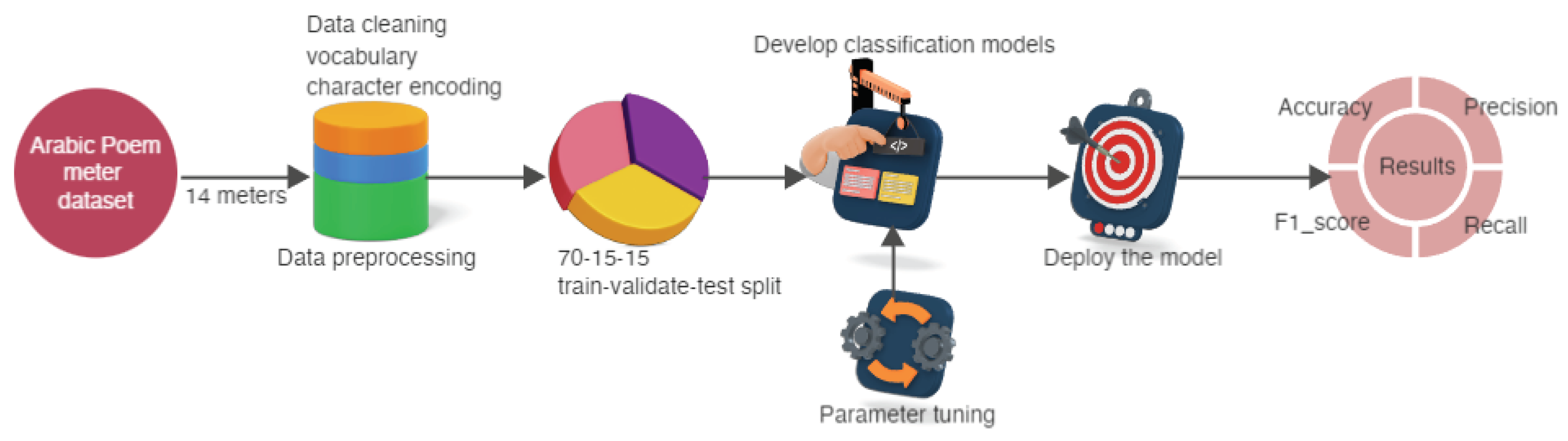
Figure 2.
The full-verse count of the 14 meters in the dataset.
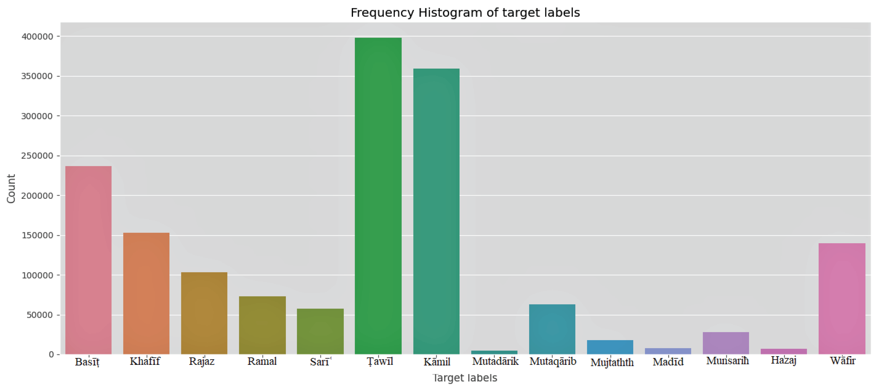
Figure 3.
Base Model with one layer. (a) LSTM model. (b) GRU model.
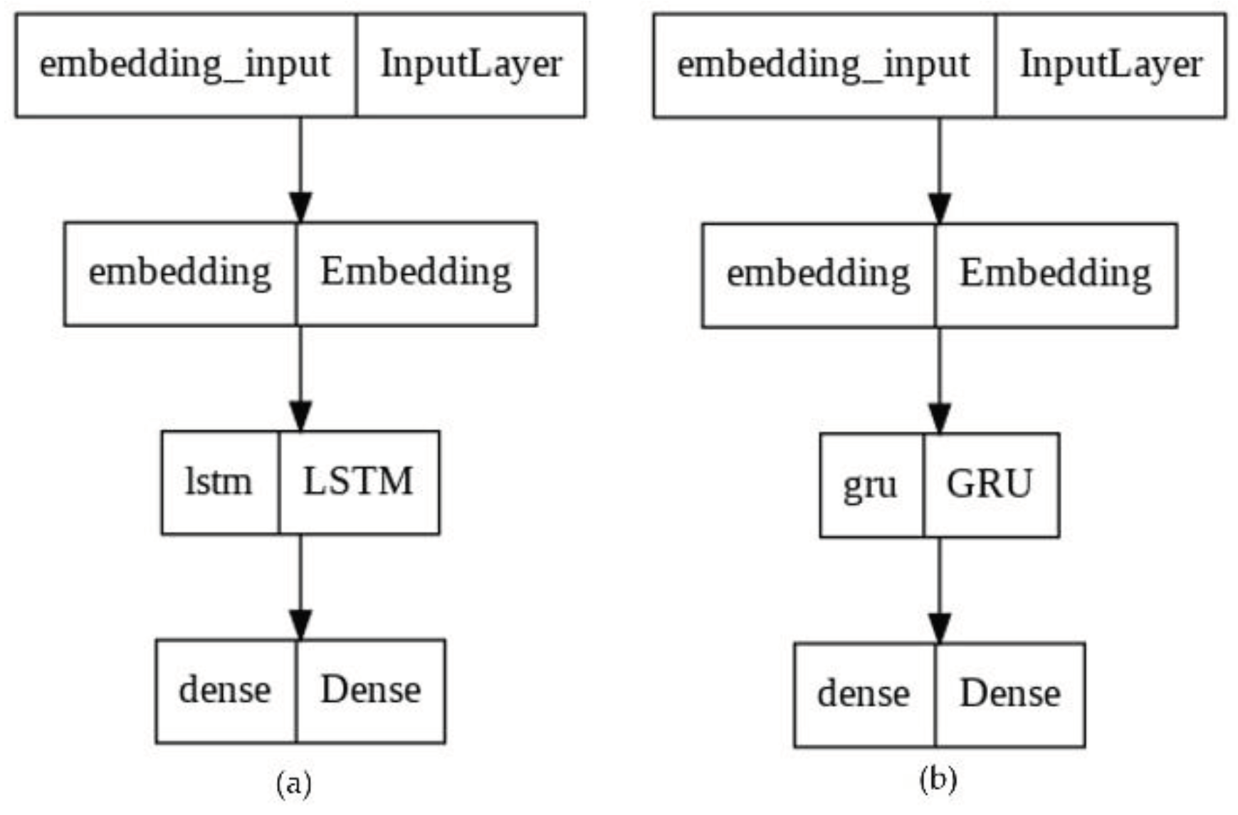
Figure 4.
The internal architecture of the LSTM layer
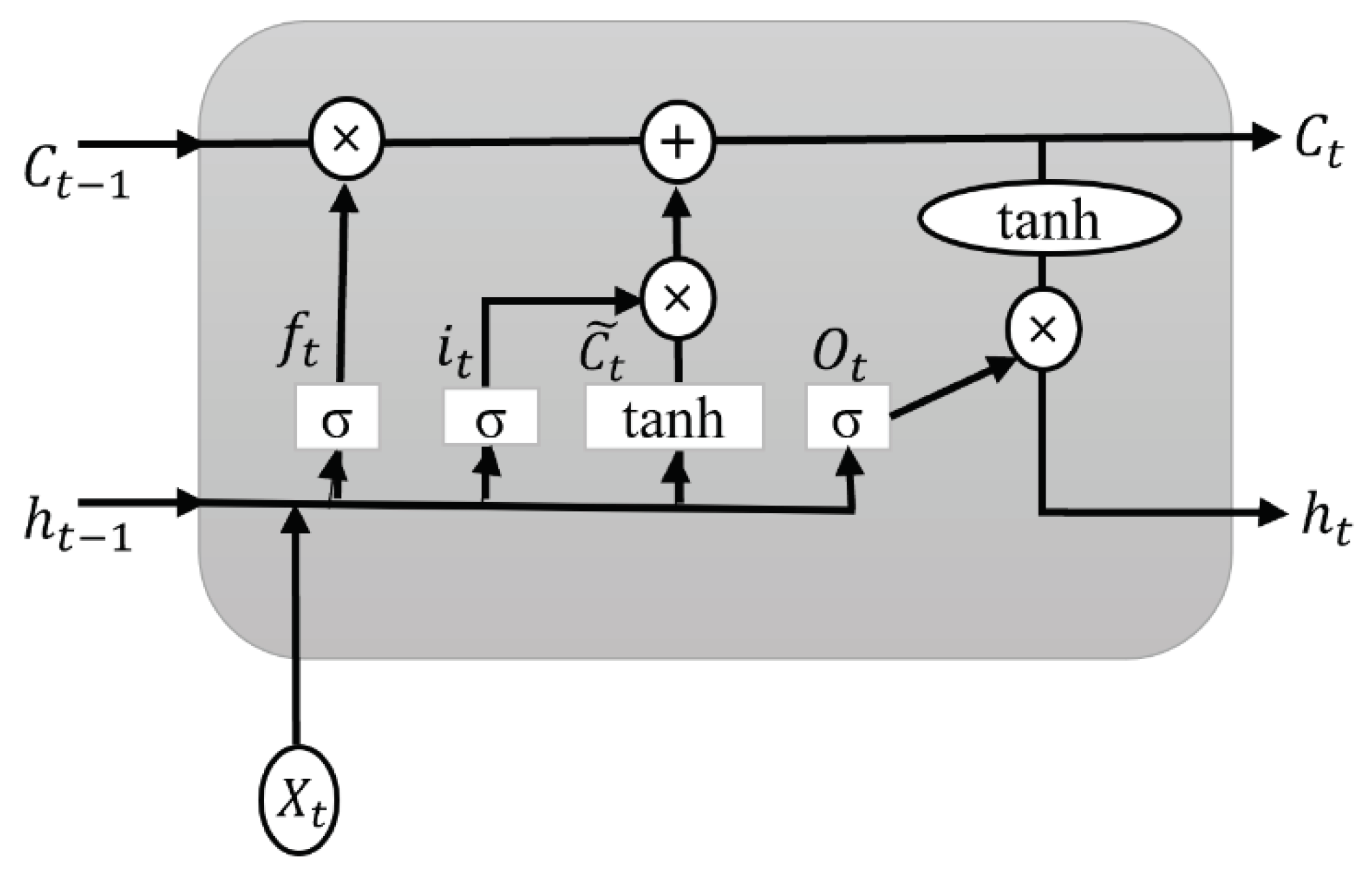
Figure 5.
The GRU layer's internal structure.
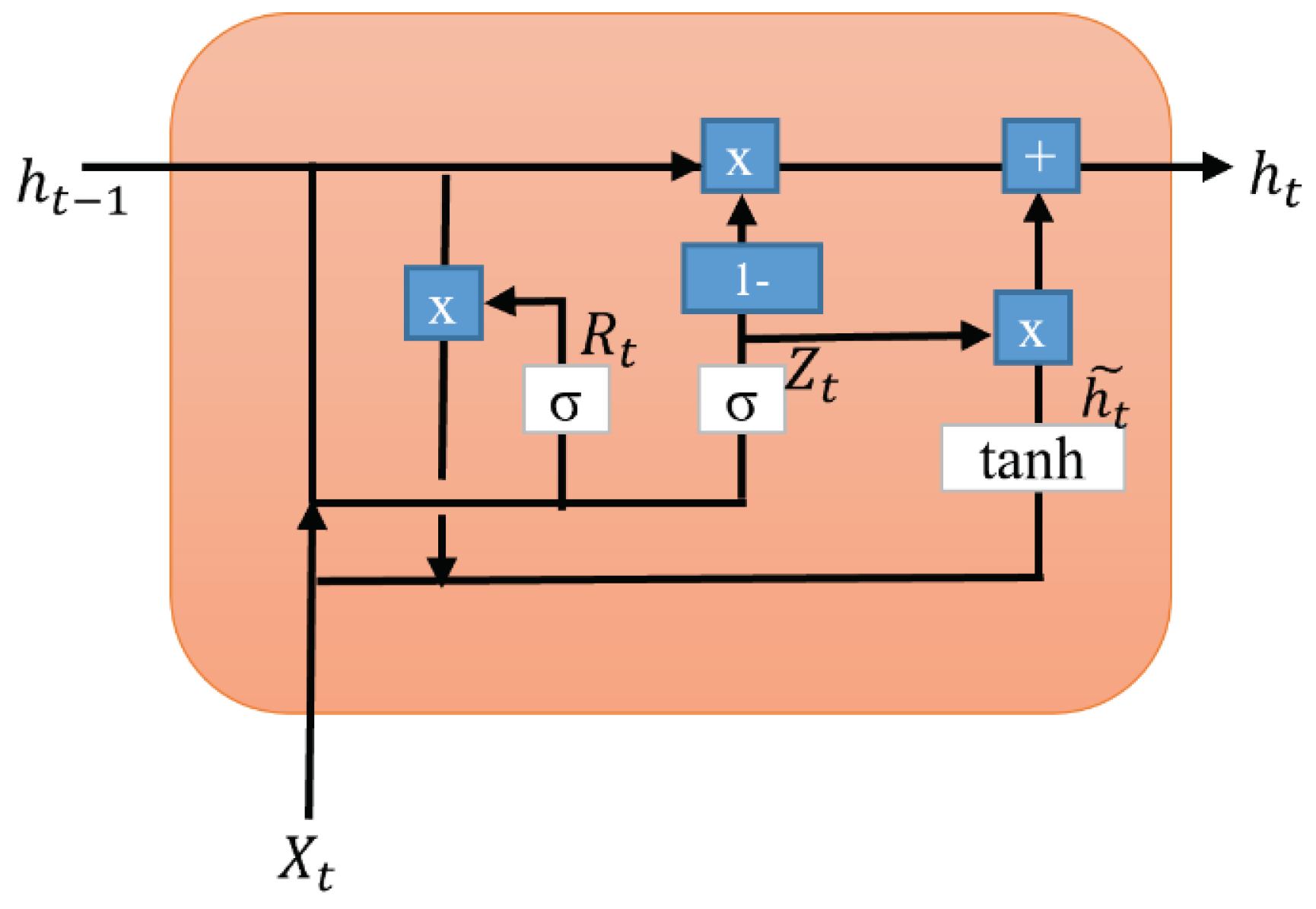
Figure 6.
Base model with one layer of BiLSTM.
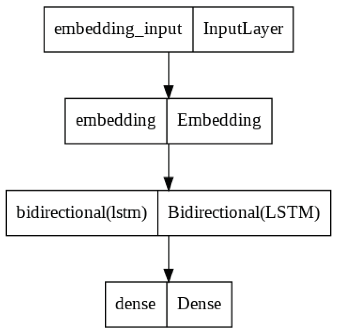
Figure 7.
The BiLSTM model architecture with two consecutive timeframes.
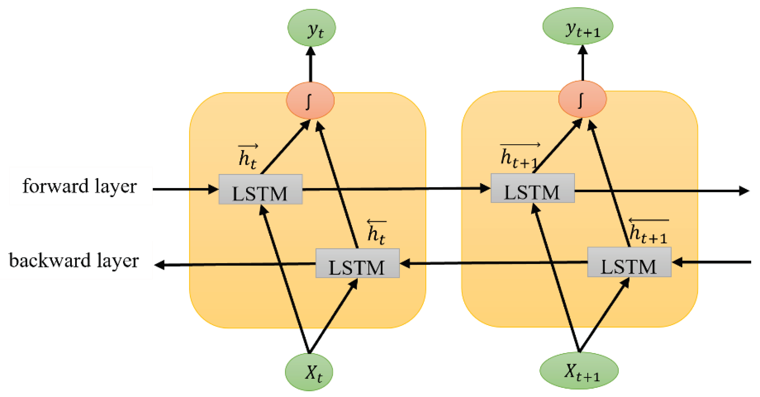
Figure 8.
Training and validation plot of BiLSTM with three layers. The left side shows the accuracy, and the right shows the loss values for each epoch.
Figure 8.
Training and validation plot of BiLSTM with three layers. The left side shows the accuracy, and the right shows the loss values for each epoch.
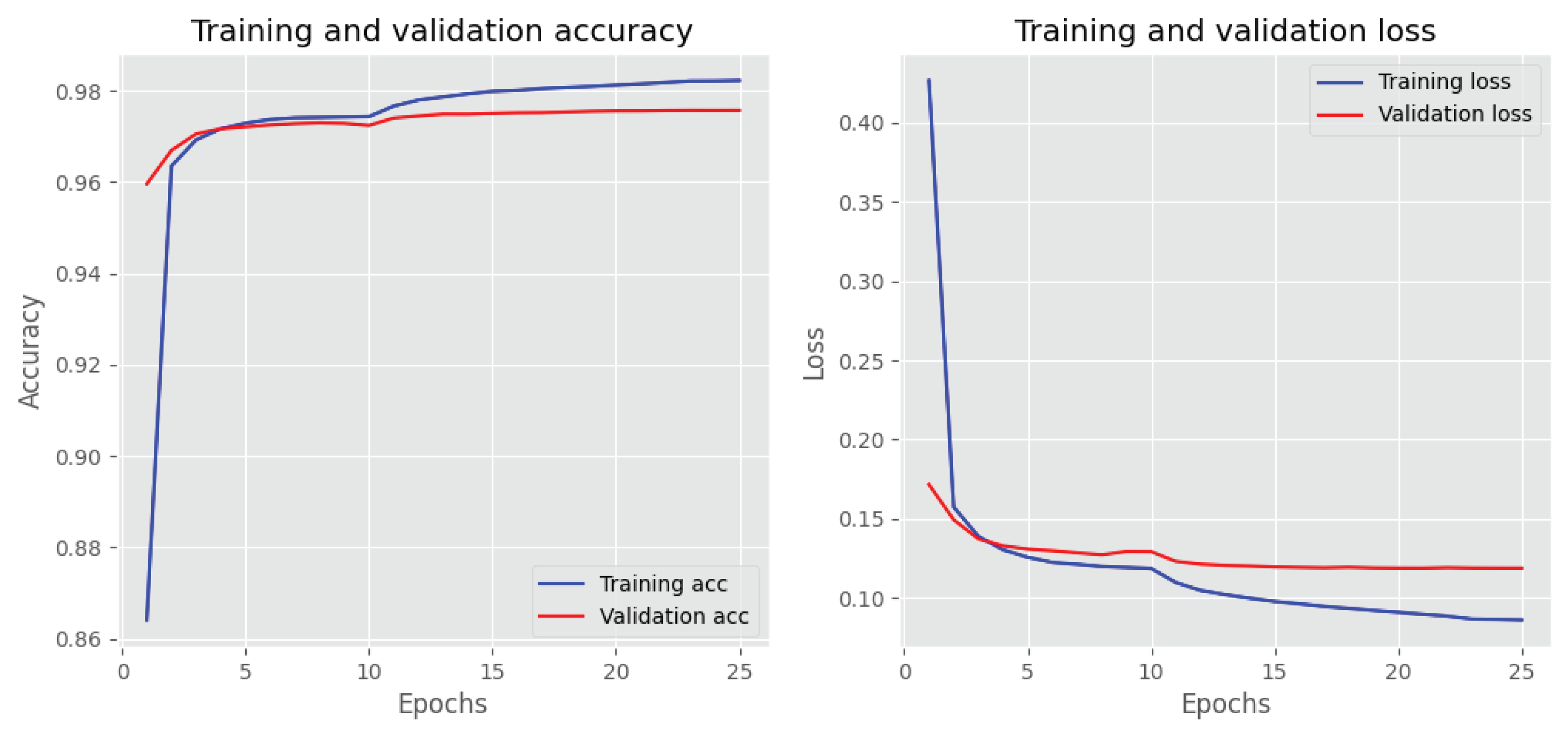
Figure 9.
Confusion matrix of three hidden layers BiLSTM model.
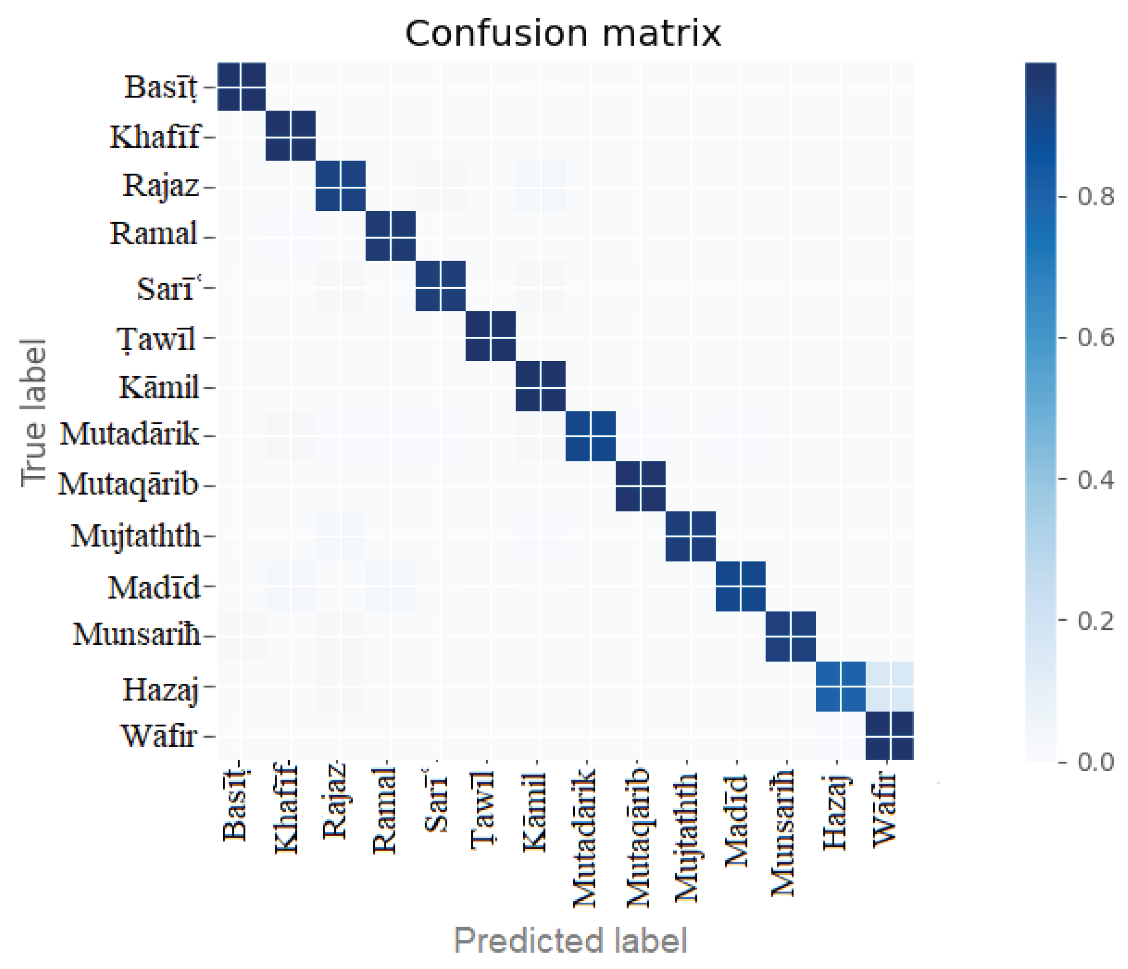
Figure 10.
Training and validation plot of BiLSTM with three layers in half-verse. The left side shows the accuracy, and the right shows the loss values for each epoch.
Figure 10.
Training and validation plot of BiLSTM with three layers in half-verse. The left side shows the accuracy, and the right shows the loss values for each epoch.
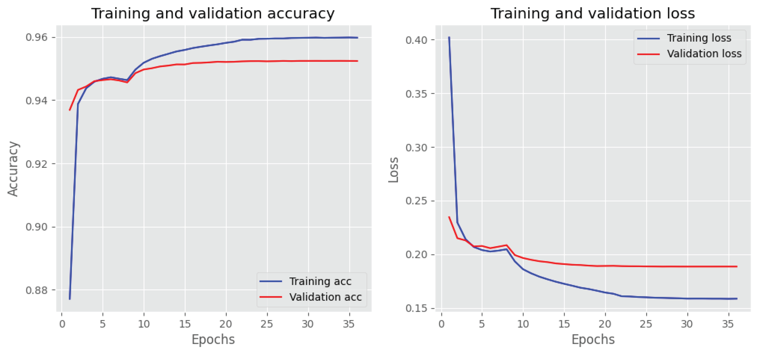
Figure 11.
Confusion matrix of half-verse BiLSTM model.
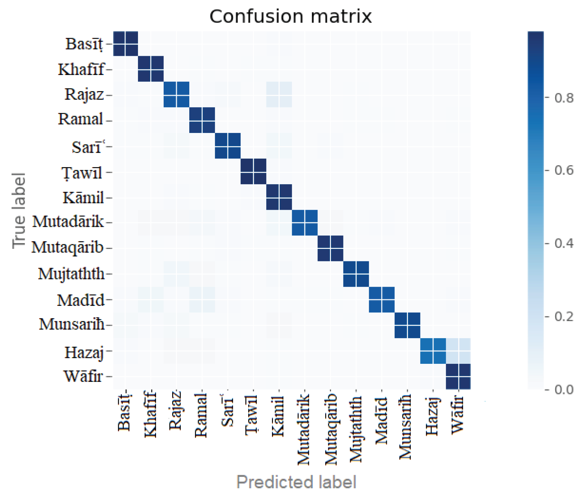

Table 1.
Arabic Diacritic types.
| Diacritic | Types | Example |
|---|---|---|
| Harakat | “fatha” “dahmmah” “kasrah” “sukon” | شَرِب الطفْلُ الحليبَ |
| Tanween | Tanween fateh, tanween dham and tanween kasr | بارداً , باردٌ , باردٍ |
| Dhawabet | Shad, mad | الشَّمس , آية |
Table 2.
Specification of the experimental setup.
| Resource | Specification |
|---|---|
| OS | Windows 10, 64-bit |
| RAM | 16 GB |
| CPU | Intel(R) Core (TM) i7-4770K @ 3.50GHz |
| GPU | Nvidia GeForce GTX 1080 Ti, Nvidia Titan V |
| Libraries with version | Python 3.9, Tensorflow 2.7, Scikit-learn 1.0, PyArabic 0.6.14 |
Table 3.
The result of increasing the layers of each model on the test accuracy of full-verse data.
| Models | Hidden layers | Parameters (in millions) | Accuracy | Training Epochs | Training Time (in hours) |
|---|---|---|---|---|---|
| LSTM | 1 | 0.34 | 0.9720 | 28 | 89.95 |
| 2 | 0.86 | 0.9733 | 26 | 148.17 | |
| 3 | 1.38 | 0.9737 | 35 | 286.15 | |
| GRU | 1 | 0.26 | 0.9710 | 28 | 166.93 |
| 2 | 0.65 | 0.9723 | 37 | 212.63 | |
| 3 | 1.05 | 0.9726 | 60 | 455.93 | |
| BiLSTM | 1 | 0.67 | 0.9698 | 19 | 110.02 |
| 2 | 2.24 | 0.9744 | 26 | 249.97 | |
| 3 | 3.82 | 0.9753 | 25 | 442.50 |
Table 4.
Performance measure of the BiLSTM model with test data.
| Meter | Precision | Recall | f1-score | Accuracy |
|---|---|---|---|---|
| Basit | 0.98 | 0.99 | 0.99 | 0.99 |
| Khafif | 0.98 | 0.98 | 0.98 | 0.98 |
| Rajaz | 0.94 | 0.93 | 0.94 | 0.93 |
| Ramal | 0.96 | 0.96 | 0.96 | 0.96 |
| Sari | 0.95 | 0.95 | 0.95 | 0.95 |
| Tawil | 0.99 | 0.99 | 0.99 | 0.99 |
| Kamil | 0.97 | 0.98 | 0.98 | 0.98 |
| Mutadarik | 0.91 | 0.90 | 0.91 | 0.90 |
| Mutaqarib | 0.98 | 0.97 | 0.98 | 0.97 |
| Mujtathth | 0.91 | 0.95 | 0.93 | 0.95 |
| Madid | 0.91 | 0.90 | 0.91 | 0.90 |
| Munsarih | 0.96 | 0.94 | 0.95 | 0.94 |
| Hazaj | 0.80 | 0.80 | 0.80 | 0.80 |
| Wafir | 0.98 | 0.98 | 0.98 | 0.98 |
Table 5.
The result of increasing the layers of each model on the test accuracy of half-verse data.
| Models | Hidden layers | Parameters (in millions) | Accuracy | Training Epochs | Training Time (in hours) |
|---|---|---|---|---|---|
| LSTM | 1 | 0.34 | 0.9465 | 34 | 153.23 |
| 2 | 0.86 | 0.9494 | 24 | 166.08 | |
| 3 | 1.39 | 0.9509 | 28 | 283.33 | |
| GRU | 1 | 0.26 | 0.9455 | 34 | 305.82 |
| 2 | 0.65 | 0.9470 | 34 | 238.78 | |
| 3 | 1.05 | 0.9459 | 60 | 667.97 | |
| BiLSTM | 1 | 0.67 | 0.9446 | 18 | 153.98 |
| 2 | 2.24 | 0.9496 | 33 | 510.00 | |
| 3 | 3.82 | 0.9523 | 36 | 711.05 |
Table 6.
Performance measure of the BiLSTM model with test data.
| Meter | Precision | Recall | f1_score | Accuracy |
|---|---|---|---|---|
| Basit | 0.98 | 0.98 | 0.98 | 0.98 |
| Khafif | 0.96 | 0.96 | 0.96 | 0.96 |
| Rajaz | 0.88 | 0.83 | 0.85 | 0.83 |
| Ramal | 0.92 | 0.93 | 0.92 | 0.93 |
| Sari | 0.91 | 0.90 | 0.90 | 0.90 |
| Tawil | 0.99 | 0.98 | 0.98 | 0.98 |
| Kamil | 0.94 | 0.96 | 0.95 | 0.96 |
| Mutadarik | 0.84 | 0.83 | 0.83 | 0.83 |
| Mutaqarib | 0.95 | 0.96 | 0.95 | 0.96 |
| Mujtathth | 0.86 | 0.89 | 0.87 | 0.89 |
| Madid | 0.84 | 0.82 | 0.83 | 0.82 |
| Munsarih | 0.93 | 0.89 | 0.91 | 0.89 |
| Hazaj | 0.71 | 0.74 | 0.73 | 0.74 |
| Wafir | 0.97 | 0.96 | 0.97 | 0.96 |
Table 7.
Comparison of related work with our study.
| Reference | Technique used | Dataset size | Accuracy |
|---|---|---|---|
| [16] | BiGRU-5 | 55,400 verses | 94.32% (full-verse), 88.80% (half-verse) |
| [4] | BiLSTM-4 | 1,657,003 verses | 97.00% (full-verse) |
| [37] | BiLSTM-7 | 1,722,321 verses | 96.38% (full-verse) |
| Our Proposed work | BiLSTM-3 | 1,646,771 verses | 97.53% (full-verse), 95.23% (half-verse) |
Disclaimer/Publisher’s Note: The statements, opinions and data contained in all publications are solely those of the individual author(s) and contributor(s) and not of MDPI and/or the editor(s). MDPI and/or the editor(s) disclaim responsibility for any injury to people or property resulting from any ideas, methods, instructions or products referred to in the content. |
© 2024 by the authors. Licensee MDPI, Basel, Switzerland. This article is an open access article distributed under the terms and conditions of the Creative Commons Attribution (CC BY) license (http://creativecommons.org/licenses/by/4.0/).
Copyright: This open access article is published under a Creative Commons CC BY 4.0 license, which permit the free download, distribution, and reuse, provided that the author and preprint are cited in any reuse.


