5th Order Multivariate Edgeworth Expansions for Parametric Estimates

1. Introduction and summary

Suppose that $\widehat{w}$ is a standard or Type A estimate of an unknown $w\in R^p$ with respect to a given parameter n. That is, $E \widehat{w}\to w$ as $n\to \infty$ and for $r\ge 1,$ its rth order cumulants have magnitude $n^{1-r}$ and can be expanded as

$$\begin{array}{c}\hfill {\overline{k}}^{1-r}=\kappa ({\widehat{w}}^{i_1},\dots ,{\widehat{w}}^{i_r})=\sum _{e=r-1}^{\infty }{n}^{-e} {\overline{k}}_e^{1-r}for1\le i_1, \dots , i_r\le p,\end{array}$$

(1)

where the cumulant coefficients ${\overline{k}}_e^{1-r}=k_e^{j_1-j_r}$ do not depend on n, or at least are bounded as $n\to \infty$. So ${\overline{k}}_0^1=w^{i_1}.$ For example (1) holds for $\widehat{w}$ a function of a sample mean. We show that if $t\left(\widehat{w}\right)$ is a smooth function of a standard estimate $\widehat{w}$, then it is a standard estimate of $t\left(w\right)$. This is done for $\widehat{w}$ unbiased in Theorem 3.1, and for $\widehat{w}$ biased in Theorem 4.1. More generally we call $\widehat{w}$ a Type B estimate if $E \widehat{w}\to w$ as $n\to \infty ,$ and for $r\ge 1$,

$$\begin{array}{c}\hfill {\overline{k}}^{1-r}=\sum _{d=2r-2}^{\infty }{n}^{-d/2} {\overline{b}}_d^{1-r}for1\le i_1, \dots , i_r\le p, {\overline{b}}_d^{1-r}=b_d^{i_1\cdots i_r}.\end{array}$$

For example this type arises when considering 1-sided confidence regions. If $t\left(\widehat{w}\right)$ is a smooth function of a Type B estimate, then it is a Type B estimate of $t\left(w\right)$. So for a Type A estimate, ${\overline{b}}_d^{1-r}$ is ${\overline{k}}_e^{1-r}$ for $d=2e$ and 0 for d odd. n is typically the sample size or the minimum sample size if there is more than one sample.

§3 and §4 show that a smooth function of $\widehat{w}$, say $t\left(\widehat{w}\right)$, is a standard estimate of $t=t\left(w\right)$. They give the cumulant coefficients of $t\left(\widehat{w}\right)$ in terms of those of $\widehat{w}$ and the derivatives of $t\left(w\right)$. §3 does this for $\widehat{w}$ unbiased and §4 for $\widehat{w}$ biased. So they can be thought of as chain rules for obtaining the cumulant coefficients for $t\left(\widehat{w}\right)$ from those of $\widehat{w}$. We give the cumulant coefficients needed for Edgeworth expansions of $\widehat{t}$ to $O\left(n^{-5/2}\right)$. Those to $O\left(n^{-1}\right)$ were given in Withers and Nadarajah (2022). Those to $O\left(n^{-r/2}\right)$ use the rth derivatives of $t\left(w\right)$. §5 specialises to univariate $t\left(w\right)$ with examples. Theorem 4.1 and Corollary 5.4 correct ${\overline{a}}_2^{12}=K_2^{j_1{j}_2}$ and $a_{22}$ on p67 and p59 of Withers (1982). §2 extends the shorthand bar notation above and gives the foundation theorem.

We now summarise the expressions for Edgeworth expansions of $\widehat{w}$ for standard and Type B estimates in terms of the cumulant coefficients ${\overline{k}}_e^{1-r}$ and ${\overline{b}}_d^{1-r}$ given in Withers and Nadarajah (2010b, 2012a, 2014a):

$$\begin{array}{cc}& Prob.(Y_{nw}\le x)=\sum _{r=0}^{\infty }{n}^{-r/2}{P}_r\left(x\right), p_{Y_{nw}}\left(x\right)=\sum _{r=0}^{\infty }{n}^{-r/2}{p}_r\left(x\right),\hfill \end{array}$$

(2)

$$\begin{array}{cc}& \mathrm{where}{Y}_{nw}=n^{1/2}(\widehat{w}-w-b_1{n}^{-1/2}), {\left(b_1\right)}_i=b_1^i, P_0\left(x\right)={\mathsf{\Phi }}_V\left(x\right),\hfill \end{array}$$

(3)

$$\begin{array}{cc}& P_r\left(x\right)={\tilde{B}}_r\left(e(-\partial /\partial x)\right) {\mathsf{\Phi }}_V\left(x\right)\mathrm{for}r\ge 1,\hfill \end{array}$$

(4)

$$\begin{array}{cc}& e_j\left(t\right)=\sum _{r=1}^{j+2} {\overline{b}}_{r+j}^{1\cdots r} t_{i_1}\cdots t_{i_r}/r!, {\overline{b}}_{r+j}^{1\cdots r}=b_{r+j}^{i_1\cdots i_r},\hfill \end{array}$$

(5)

${\mathsf{\Phi }}_V\left(x\right)$ is the multivariate normal distribution with zero mean and covariance $V=\left({\overline{b}}_2^{12}\right)$, ${\tilde{B}}_r\left(e\right)$ is the complete ordinary Bell polynomial of Comtet (1974):

$$\begin{array}{cc}& {\tilde{B}}_1\left(e\right)=e_1, {\tilde{B}}_2\left(e\right)=e_2+e_1^2, {\tilde{B}}_3\left(e\right)=e_3+2e_1{e}_2+e_1^3,\hfill \\ & {\tilde{B}}_4\left(e\right)=e_4+2e_1{e}_3+e_2^2+3e_1^2{e}_2+e_1^4.\hfill \end{array}$$

This gives the 5th order Edgeworth expansion for the distribution of $Y_{nw}$, that is, it gives (2) to $O\left(n^{-5/2}\right)$. Note that (5) uses the tensor summation convention of implicitly summing $i_1,\cdots ,i_r$ over their range $1,\cdots ,p$. For example

$$\begin{array}{cc}& \mathrm{for}{\partial }_i=\partial /\partial x_i\mathrm{and}{\overline{\partial }}_k={\partial }_{i_k},\hfill \\ & P_1\left(x\right)=e_1(-\partial /\partial x)) {\mathsf{\Phi }}_V\left(x\right)=\sum _{r=1}^3{\overline{b}}_{r+1}^{1\cdots r} (-{\overline{\partial }}_1)\cdots (-{\overline{\partial }}_r) {\mathsf{\Phi }}_V\left(x\right)\hfill \\ & ={\overline{k}}_1^1 (-{\overline{\partial }}_1) {\mathsf{\Phi }}_V\left(x\right)+{\overline{k}}_2^{1-3} (-{\overline{\partial }}_1)(-{\overline{\partial }}_2)(-{\overline{\partial }}_3) {\mathsf{\Phi }}_V\left(x\right)\hfill \end{array}$$

for a standard estimate. For a standard estimate, $b_1=0$ in (3) and the cumulant coefficients needed for $P_r\left(x\right),p_r\left(x\right)$ of (2) are ${\overline{k}}_0^1=w^{i_1}$,

$$\begin{array}{cc}& \mathrm{for}r=0: {\overline{k}}_1^{12}; \mathrm{for}r=1: {\overline{k}}_1^1, {\overline{k}}_2^{1-3}; \mathrm{for}r=2: {\overline{k}}_2^{12}, {\overline{k}}_3^{1-4};\hfill \end{array}$$

(6)

(7)

So to obtain the 5th order Edgeworth expansion for the distribution of $n^{1/2}(t\left(\widehat{w}\right)-t\left(w\right))$ for $\widehat{w}$ a standard estimate, we just need to replace the coefficients in (6) and (7) where they appear in $P_r\left(x\right), r\le 4$, by those of $t\left(\widehat{w}\right)$ given in §3-§5.

(9) of Withers and Nadarajah (2010b) gives $P_r\left(x\right)$ for the more general case where $P_0\left(x\right)$ is the distribution function of $Y\in R^p$ which depends on n but is asymptotic to ${\mathsf{\Phi }}_V\left(x\right)$ and has a Type B expansion. One can choose $P_0\left(x\right)$ so that the number of terms in each $P_r\left(x\right)$ greatly reduces: see Withers and Nadarajah (2012d, 2014c, 2015). When $\widehat{w}$ is lattice, further terms need to be added: see for example Chapter 5 of Bhattacharya and Rao (1976), Cai (2005), and for the density of $Y_{nw}$, p211 of Barndoff-Nielsen and Cox (1989), §5 of Daniels (1983), and §6 of Daniels (1987). Corollary 1 of Withers and Nadarajah (2010b) gives the tilted Edgeworth expansion for $t\left(\widehat{w}\right)$, sometimes called the saddlepoint approximation, or the small sample expansion as it is a series in $n^{-1}$ not just $n^{-1/2}$. It is very useful for the tails of the distribution where Edgeworth expansions perform poorly. Cumulant coefficients are also needed for bias reduction, Bayesian inference, confidence regions and power. See Withers (1984) and Withers and Nadarajah (2008, 2010a, 2011b, 2011c, 2012b, 2012f, 2014b, 2014c, 2015) for examples. For a history of Edgeworth expansions, see §7.

In summary, this paper gives high order expansions for the distribution of a vast range of estimates, by obtaining the cumulant coefficients needed for any smooth function of a standard estimate. This provides unprecedented accuracy for these distributions and avoids the need for simulation methods.

2. Foundations

Given $w=(w^1,\cdots ,w^p)\in R^p$ and an estimate $\widehat{w},$ suppose that $E \widehat{w}\to w$ as $n\to \infty$ and that for $r\ge 1,$ its rth order cumulants have magnitude $n^{1-r}$. Given $i_1,\cdots ,i_r$ in $1,2,\cdots ,p$, we write these cumulants in shorthand as

$$\begin{array}{c}\hfill {\overline{k}}^{1-r}=k^{i_1\cdots i_r}=\kappa ({\widehat{w}}^{i_1},\dots ,{\widehat{w}}^{i_r})=O\left(n^{1-r}\right)\mathrm{as}n\to \infty .\end{array}$$

(1)

For example if $\widehat{w}=\overline{X}$ is the mean of a random sample of size n, then (1) holds since ${\overline{k}}^{1-r}=n^{1-r}\kappa (X^{i_1},\dots ,X^{i_r})$ where $X^i$ is the ith component of X. By Theorem 2.1, (1) holds if $\widehat{w}$ is a smooth function of one or more sample means. Let $t:R^p\to R^q$ be a smooth function in a neighbourhood of w with jth component $t^j=t^j\left(w\right), j=1,\cdots ,q$ and finite partial derivatives

$${\overline{t}}_{sr\cdots }^k=t_{\cdot i_s{i}_r\cdots }^{j_k}={\partial }_{i_s}{\partial }_{i_r}\cdots t^{j_k}\left(w\right), {\overline{t}}_{s-r}^k=t_{\cdot i_s\cdots i_r}^{j_k}fors\le r$$

where ${\partial }_i=\partial /\partial w^i.$ We reserve i’s as superscripts for the cumulants of $\widehat{w}$ and subscripts for partial derivatives of $t\left(w\right)$. We reserve j’s as superscripts for the components of $t\left(w\right)$ and for the joint cumulants of $\widehat{t}=t\left(\widehat{w}\right)$. This bar shorthand allows us to shorten expressions by suppressing the i’s and j’s. We write the cumulants of $\widehat{t}=t\left(\widehat{w}\right)$ as

$$\begin{array}{c}\hfill {\overline{K}}^{1-r}=K^{j_1\cdots j_r}=\kappa ({\widehat{t}}^{j_1},\dots ,{\widehat{t}}^{j_r})\mathrm{where}\widehat{t}=t\left(\widehat{w}\right), {\widehat{t}}^j=t^j\left(\widehat{w}\right).\end{array}$$

(2)

For example

$$\begin{array}{cc}& {\overline{k}}^{12}=k^{i_1{i}_2}, {\overline{K}}^{12}=K^{j_1{j}_2}\Rightarrow covar\left(\widehat{w}\right)=\left({\overline{k}}^{12}\right),\mathrm{and}covar\left(\widehat{t}\right)=\left({\overline{K}}^{12}\right).\hfill \end{array}$$

are $O\left(n^{-1}\right)$. We now show that

$$\begin{array}{cc}& {\overline{K}}^{12}={ }_1{\overline{K}}^{12}+O\left(n^{-2}\right){where}_1{\overline{K}}^{12}={\overline{t}}_1^1{\overline{t}}_2^2 {\overline{k}}^{12},{thatis,}_1{K}^{j_1{j}_2}=t_{\cdot i_1}^{j_1}{t}_{\cdot i_2}^{j_2}{k}^{i_1{i}_2},\hfill \end{array}$$

using the tensor sum convention. The rest of this section and all proofs can be skipped on a 1st reading. Theorem 2.1 gives the cumulants of $\widehat{t}=t\left(\widehat{w}\right)$ when $\widehat{w}$ is unbiased.

We shall use the notation ${\sum }^N{f}^{j_1{j}_2\cdots }$ to mean summing over all N permutations of $j_1,j_2,\cdots$ giving distinct terms.

Theorem 1. 

Suppose that $E \widehat{w}=w$ and that (1) holds. Then for $r\ge 1$ and $1\le j_1, \dots , j_r\le q, {\overline{K}}^{1-r}$ of (2) satisfies

$$\begin{array}{cc}& {\overline{K}}^{1-r}=\sum _{e=r-1}^{\infty }{ }_e{\overline{K}}^{1-r}where{ }_e{\overline{K}}^{1-r}={ }_e{K}^{j_1\cdots j_r}=O\left(n^{-e}\right)asn\to \infty ,\hfill \end{array}$$

(3)

and the leading ${ }_e{\overline{K}}^{1-r}$ are as follows.

$$\begin{array}{cc}& { }_0{\overline{K}}^1={\overline{t}}^1,{thatis,}_0{K}^{j_1}=t^{j_1},\hfill \\ & { }_1{\overline{K}}^1={\overline{t}}_{12}^1{\overline{k}}^{12}/2,thatis,{ }_1{K}^{j_1}=t_{\cdot i_1{i}_2}^{j_1} k^{i_1{i}_2}/2=\sum _{i_1,i_2=1}^p{t}_{\cdot i_1{i}_2}^{j_1} k^{i_1{i}_2}/2,\hfill \\ & { }_2{\overline{K}}^1={\overline{t}}_{1-3}^1 {\overline{k}}^{1-3}/6+{\overline{t}}_{1-4}^1 {\overline{k}}^{12}{\overline{k}}^{34}/8,\hfill & \\ & {thatis,}_2{K}^{j_1}=t_{\cdot i_1{i}_2{i}_3}^{j_1}{k}^{i_1{i}_2{i}_3}/6+t_{\cdot i_1-i_4}^{j_1}{\overline{k}}^{i_1{i}_2}{\overline{k}}^{i_3{i}_4}/8,\hfill \\ & { }_3{\overline{K}}^1={\overline{t}}_{1-4}^1{\overline{k}}^{1-4}/24+{\overline{t}}_{1-5}^1{\overline{k}}^{1-3}{\overline{k}}^{45}/12+{\overline{t}}_{1-6}^1 {\overline{k}}^{12}{\overline{k}}^{34}{\overline{k}}^{56}/48,\hfill \\ & { }_4{\overline{K}}^1={\overline{t}}_{1-5}^1{\overline{k}}^{1-5}/120+{\overline{t}}_{1-6}^1 ({\overline{k}}^{1-4}{\overline{k}}^{56}/48+{\overline{k}}^{1-3}{\overline{k}}^{4-6}/72)+{\overline{t}}_{1-7}^1 {\overline{k}}^{1-3}{\overline{k}}^{45}{\overline{k}}^{67}/48\hfill \\ & +{\overline{t}}_{1-8}^1 {\overline{k}}^{12}{\overline{k}}^{34}{\overline{k}}^{56}{\overline{k}}^{78}/384,\hfill \end{array}$$

$$\begin{array}{cc}& { }_1{\overline{K}}^{12}={\overline{t}}_1^1{\overline{t}}_2^2 {\overline{k}}^{12},{ }_2{\overline{K}}^{12}=T_{1-3}^{12} {\overline{k}}^{1-3}/2+T_{1-4}^{12} {\overline{k}}^{12}{\overline{k}}^{34}/2where\hfill \\ & T_{1-3}^{12}=\sum ^2{\overline{t}}_{12}^1{\overline{t}}_3^2, T_{1-4}^{12}=\sum ^2{\overline{t}}_{1-3}^1{\overline{t}}_4^2+{\overline{t}}_{13}^1{\overline{t}}_{24}^2, \sum ^2{\overline{t}}_{a-b}^1{\overline{t}}_{c-d}^2={\overline{t}}_{a-b}^1{\overline{t}}_{c-d}^2+{\overline{t}}_{a-b}^2{\overline{t}}_{c-d}^1,\hfill \\ & { }_3{\overline{K}}^{12}=U_{1-4}^{12} {\overline{k}}^{1-4}+T_{1-5}^{12} {\overline{k}}^{1-3}{\overline{k}}^{45}+T_{1-6}^{12} {\overline{k}}^{12}{\overline{k}}^{34}{\overline{k}}^{56}/4where\hfill \\ & U_{1-4}^{12}=\sum ^2{\overline{t}}_{1-3}^1{\overline{t}}_4^2/6+{\overline{t}}_{12}^1{\overline{t}}_{34}^2/4,\hfill \\ & T_{1-5}^{12}=\sum ^2({\overline{t}}_{1-4}^1{\overline{t}}_5^2/6+{\overline{t}}_{1245}^1{\overline{t}}_3^2/4+{\overline{t}}_{124}^1{\overline{t}}_{35}^2/2+{\overline{t}}_{1455}^1{\overline{t}}_{23}^2/4),\hfill \\ & T_{1-6}^{12}=\sum ^2{\overline{t}}_{1-5}^1{\overline{t}}_6^2/2+\sum ^2{\overline{t}}_{1235}^1{\overline{t}}_{46}^2+{\overline{t}}_{1-3}^1{\overline{t}}_{4-6}^2+2{\overline{t}}_{1355}^1{\overline{t}}_{246}^1/3,\hfill \\ & { }_2{\overline{K}}^{1-3}={\overline{t}}_1^1{\overline{t}}_2^2{\overline{t}}_3^3 {\overline{k}}^{1-3}+T_{1-4}^{1-3} {\overline{k}}^{12}{\overline{k}}^{34}where{T}_{1-4}^{1-3}=\sum ^3{\overline{t}}_{13}^1{\overline{t}}_2^2{\overline{t}}_4^3,\hfill \\ & { }_3{\overline{K}}^{1-3}=T_{1-4}^{1-3} {\overline{k}}^{1-4}/2+T_{1-5}^{1-3} {\overline{k}}^{1-3}{\overline{k}}^{45}+T_{1-6}^{1-3} {\overline{k}}^{12}{\overline{k}}^{34}{\overline{k}}^{56}where\hfill \\ & T_{1-5}^{1-3}=\sum ^6{\overline{t}}_{124}^1{\overline{t}}_3^2{\overline{t}}_5^3/2+\sum ^3{\overline{t}}_{145}^1{\overline{t}}_2^2{\overline{t}}_3^3/2+\sum ^6{\overline{t}}_{12}^1{\overline{t}}_{34}^2{\overline{t}}_5^3/2+\sum ^3{\overline{t}}_{14}^1{\overline{t}}_{25}^2{\overline{t}}_3^3,\hfill \\ & T_{1-6}^{1-3}=\sum ^3{\overline{t}}_{1235}^1{\overline{t}}_4^2{\overline{t}}_6^3/2+\sum ^6{\overline{t}}_{1-3}^1{\overline{t}}_{45}^2{\overline{t}}_6^3+\sum ^6{\overline{t}}_{135}^1{\overline{t}}_{24}^2{\overline{t}}_6^3/2+{\overline{t}}_{13}^1{\overline{t}}_{25}^2{\overline{t}}_{46}^3,\hfill \\ & { }_3{\overline{K}}^{1-4}={\overline{t}}_1^1\cdots {\overline{t}}_4^4 {\overline{k}}^{1-4}+T_{1-5}^{1-4} {\overline{k}}^{1-3}{\overline{k}}^{45}+T_{1-6}^{1-4} {\overline{k}}^{12}{\overline{k}}^{34}{\overline{k}}^{56}where\hfill \\ & T_{1-5}^{1-4}=\sum ^{12}{\overline{t}}_{14}^1{\overline{t}}_2^2{\overline{t}}_3^3{\overline{t}}_5^4, T_{1-6}^{1-4}=\sum ^4{\overline{t}}_{135}^1{\overline{t}}_2^2{\overline{t}}_4^3{\overline{t}}_6^4+\sum ^{12}{\overline{t}}_{13}^1{\overline{t}}_{25}^2{\overline{t}}_4^3{\overline{t}}_6^4,\hfill \\ & { }_4{\overline{K}}^{1-4}=U_{1-5}^{1-4} {\overline{k}}^{1-5}/2+U_{1-6}^{1-4} {\overline{k}}^{1-4}{\overline{k}}^{56}+V_{1-6}^{1-4} {\overline{k}}^{1-3}{\overline{k}}^{4-6}+T_{1-7}^{1-4} {\overline{k}}^{1-3}{\overline{k}}^{45}{\overline{k}}^{67}\hfill \\ & +T_{1-8}^{1-4} {\overline{k}}^{12}{\overline{k}}^{34}{\overline{k}}^{56}{\overline{k}}^{78}where{U}_{1-5}^{1-4}=\sum ^4{\overline{t}}_{12}^1{\overline{t}}_3^2{\overline{t}}_4^3{\overline{t}}_5^4,\hfill \\ & U_{1-6}^{1-4}=\sum ^{12}{\overline{t}}_{125}^1{\overline{t}}_3^2{\overline{t}}_4^3{\overline{t}}_6^4/2+\sum ^4{\overline{t}}_{156}^1{\overline{t}}_2^2{\overline{t}}_3^3{\overline{t}}_4^4/2+\sum ^{24}{\overline{t}}_{12}^1{\overline{t}}_{35}^2{\overline{t}}_4^3{\overline{t}}_6^4/2+\sum ^6{\overline{t}}_{15}^1{\overline{t}}_{26}^2{\overline{t}}_3^3{\overline{t}}_4^4),\hfill \\ & V_{1-6}^{1-4}=\sum ^{12}{\overline{t}}_{124}^1{\overline{t}}_3^2{\overline{t}}_5^3{\overline{t}}_6^4/2+\sum ^{12}{\overline{t}}_{12}^1{\overline{t}}_{34}^2{\overline{t}}_5^3{\overline{t}}_6^4/2+\sum ^6{\overline{t}}_{14}^1{\overline{t}}_{25}^2{\overline{t}}_3^3{\overline{t}}_6^4,\hfill \\ & T_{1-7}^{1-4}=\sum ^{12}{\overline{t}}_{1246}^1{\overline{t}}_3^2{\overline{t}}_5^3{\overline{t}}_7^4/2+\sum ^{12}{\overline{t}}_{1456}^1{\overline{t}}_2^2{\overline{t}}_3^3{\overline{t}}_7^4/2+\sum ^{24}{\overline{t}}_{124}^1{\overline{t}}_{36}^2{\overline{t}}_5^3{\overline{t}}_7^4/2+\sum ^{24}{\overline{t}}_{124}^1{\overline{t}}_{56}^2{\overline{t}}_3^3{\overline{t}}_7^4/2\hfill \\ & +\sum ^{24}{\overline{t}}_{145}^1{\overline{t}}_{26}^2{\overline{t}}_3^3{\overline{t}}_7^4/2+\sum ^{12}{\overline{t}}_{146}^1{\overline{t}}_{23}^2{\overline{t}}_5^3{\overline{t}}_7^4+\sum ^{24}{\overline{t}}_{146}^1{\overline{t}}_{25}^2{\overline{t}}_3^3{\overline{t}}_7^4+\sum ^{12}{\overline{t}}_{146}^1{\overline{t}}_{57}^2{\overline{t}}_2^3{\overline{t}}_3^4/2\hfill \\ & +\sum ^{12}{\overline{t}}_{456}^1{\overline{t}}_{17}^2{\overline{t}}_2^3{\overline{t}}_3^4+\sum ^{24}{\overline{t}}_{12}^1{\overline{t}}_{34}^2{\overline{t}}_{56}^3{\overline{t}}_7^4/2+\sum ^{12}{\overline{t}}_{14}^1{\overline{t}}_{25}^2{\overline{t}}_{36}^3{\overline{t}}_7^4+\sum ^{12}{\overline{t}}_{14}^1{\overline{t}}_{26}^2{\overline{t}}_{57}^3{\overline{t}}_3^4),,\hfill \\ & T_{1-8}^{1-4}=\sum ^4{\overline{t}}_{12357}^1{\overline{t}}_4^2{\overline{t}}_6^3{\overline{t}}_8^4/2+\sum ^{24}{\overline{t}}_{1235}^1{\overline{t}}_{47}^2{\overline{t}}_6^3{\overline{t}}_8^4/2+\sum ^{12}{\overline{t}}_{1357}^1{\overline{t}}_{24}^2{\overline{t}}_6^3{\overline{t}}_8^4/2\hfill \\ & +\sum ^{12}{\overline{t}}_{123}^1{\overline{t}}_{457}^2{\overline{t}}_6^3{\overline{t}}_8^4/2+\sum ^{12}{\overline{t}}_{135}^1{\overline{t}}_{247}^2{\overline{t}}_6^3{\overline{t}}_8^4/2+\sum ^{24}{\overline{t}}_{123}^1{\overline{t}}_{45}^2{\overline{t}}_{67}^3{\overline{t}}_8^4/2+\sum ^{24}{\overline{t}}_{135}^1{\overline{t}}_{24}^2{\overline{t}}_{67}^3{\overline{t}}_8^4\hfill \end{array}$$

$$\begin{array}{cc}& +\sum ^{12}{\overline{t}}_{135}^1{\overline{t}}_{27}^2{\overline{t}}_{48}^3{\overline{t}}_6^4/2+\sum ^3{\overline{t}}_{13}^1{\overline{t}}_{25}^2{\overline{t}}_{47}^3{\overline{t}}_{68}^4,\hfill \\ & { }_4{\overline{K}}^{1-5}={\overline{t}}_1^1\cdots {\overline{t}}_5^5 {\overline{k}}^{1-5}+T_{1-6}^{1-5} {\overline{k}}^{1-4}{\overline{k}}^{56}+U_{1-6}^{1-5} {\overline{k}}^{1-3}{\overline{k}}^{4-6}+T_{1-7}^{1-5} {\overline{k}}^{1-3}{\overline{k}}^{45}{\overline{k}}^{67}\hfill \\ & +T_{1-8}^{1-5} {\overline{k}}^{12}{\overline{k}}^{34}{\overline{k}}^{56}{\overline{k}}^{78}where\hfill \\ & T_{1-6}^{1-5}=\sum ^{20}{\overline{t}}_{15}^1{\overline{t}}_2^2{\overline{t}}_3^3{\overline{t}}_4^4{\overline{t}}_6^5, U_{1-6}^{1-5}=\sum ^{15}{\overline{t}}_{14}^1{\overline{t}}_2^2{\overline{t}}_3^3{\overline{t}}_5^4{\overline{t}}_6^5,\hfill \\ & T_{1-7}^{1-5}=\sum ^{30}{\overline{t}}_{146}^1{\overline{t}}_2^2{\overline{t}}_3^3{\overline{t}}_5^4{\overline{t}}_7^5+\sum ^{60}{\overline{t}}_{14}^1{\overline{t}}_{26}^2{\overline{t}}_3^3{\overline{t}}_5^4{\overline{t}}_7^5+\sum ^{60}{\overline{t}}_{14}^1{\overline{t}}_{56}^2{\overline{t}}_2^3{\overline{t}}_3^4{\overline{t}}_7^5,\hfill \\ & T_{1-8}^{1-5}=\sum ^5{\overline{t}}_{1357}^1{\overline{t}}_2^2{\overline{t}}_4^3{\overline{t}}_6^4{\overline{t}}_8^5/5+\sum ^{60}{\overline{t}}_{135}^1{\overline{t}}_{27}^2{\overline{t}}_4^3{\overline{t}}_6^4{\overline{t}}_8^5+\sum ^{60}{\overline{t}}_{13}^1{\overline{t}}_{25}^2{\overline{t}}_{47}^3{\overline{t}}_6^4{\overline{t}}_8^5,\hfill \\ & { }_5{\overline{K}}^{1-6}={\overline{t}}_1^1\cdots {\overline{t}}_6^5 {\overline{k}}^{1-6}+T_{1-7}^{1-6} {\overline{k}}^{1-5}{\overline{k}}^{67}+U_{1-7}^{1-6} {\overline{k}}^{1-4}{\overline{k}}^{5-7}+T_{1-8}^{1-6} {\overline{k}}^{1-4}{\overline{k}}^{56}{\overline{k}}^{78}\hfill \\ & +U_{1-8}^{1-6} {\overline{k}}^{1-3}{\overline{k}}^{4-6}{\overline{k}}^{78}+T_{1-9}^{1-6} {\overline{k}}^{1-3}{\overline{k}}^{45}{\overline{k}}^{67}{\overline{k}}^{89}+T_{1-10}^{1-6} {\overline{k}}^{12}{\overline{k}}^{34}{\overline{k}}^{56}{\overline{k}}^{78}{\overline{k}}^{9,10}where\hfill \\ & T_{1-7}^{1-6}=\sum ^{30}{\overline{t}}_{16}^1{\overline{t}}_2^2{\overline{t}}_3^3{\overline{t}}_4^4{\overline{t}}_5^5{\overline{t}}_7^6, U_{1-7}^{1-6}=\sum ^{60}{\overline{t}}_{15}^1{\overline{t}}_2^2{\overline{t}}_3^3{\overline{t}}_4^4{\overline{t}}_6^5{\overline{t}}_7^6,\hfill \\ & T_{1-8}^{1-6}=\sum ^{60}{\overline{t}}_{157}^1{\overline{t}}_2^2{\overline{t}}_3^3{\overline{t}}_4^4{\overline{t}}_6^5{\overline{t}}_8^6+\sum ^{180}{\overline{t}}_{15}^1{\overline{t}}_{27}^2{\overline{t}}_3^3{\overline{t}}_4^4{\overline{t}}_6^5{\overline{t}}_8^6+\sum ^{120}{\overline{t}}_{15}^1{\overline{t}}_{67}^2{\overline{t}}_2^3{\overline{t}}_3^4{\overline{t}}_4^5{\overline{t}}_8^6,\hfill \\ & U_{1-8}^{1-6}=\sum ^{90}{\overline{t}}_{147}^1{\overline{t}}_2^2{\overline{t}}_3^3{\overline{t}}_5^4{\overline{t}}_6^5{\overline{t}}_8^6+\sum ^{360}{\overline{t}}_{14}^1{\overline{t}}_{27}^2{\overline{t}}_3^3{\overline{t}}_5^4{\overline{t}}_6^5{\overline{t}}_8^6+\sum ^{90}{\overline{t}}_{17}^1{\overline{t}}_{48}^2{\overline{t}}_2^3{\overline{t}}_3^4{\overline{t}}_5^5{\overline{t}}_6^6,\hfill \\ & T_{1-9}^{1-6}=\sum ^{60}{\overline{t}}_{1468}^1{\overline{t}}_2^2{\overline{t}}_3^3{\overline{t}}_5^4{\overline{t}}_7^5{\overline{t}}_9^6+\sum ^{360}{\overline{t}}_{146}^1{\overline{t}}_{28}^2{\overline{t}}_3^3{\overline{t}}_5^4{\overline{t}}_7^5{\overline{t}}_9^6+\sum ^{360}{\overline{t}}_{146}^1{\overline{t}}_{58}^2{\overline{t}}_2^3{\overline{t}}_3^4{\overline{t}}_7^5{\overline{t}}_9^6\hfill \\ & +\sum ^{180}{\overline{t}}_{468}^1{\overline{t}}_{15}^2{\overline{t}}_2^3{\overline{t}}_3^4{\overline{t}}_7^5{\overline{t}}_9^6+\sum ^{120}{\overline{t}}_{14}^1{\overline{t}}_{26}^2{\overline{t}}_{38}^3{\overline{t}}_5^4{\overline{t}}_7^5{\overline{t}}_9^6+\sum ^{720}{\overline{t}}_{14}^1{\overline{t}}_{26}^2{\overline{t}}_{58}^3{\overline{t}}_3^4{\overline{t}}_7^5{\overline{t}}_9^6\hfill \\ & +\sum ^{360}{\overline{t}}_{14}^1{\overline{t}}_{56}^2{\overline{t}}_{78}^3{\overline{t}}_2^4{\overline{t}}_3^5{\overline{t}}_9^6,\hfill \\ & T_{1-10}^{1-6}=\sum ^6{\overline{t}}_{13579}^1{\overline{t}}_2^2{\overline{t}}_4^3{\overline{t}}_6^4{\overline{t}}_8^5{\overline{t}}_{10}^6+\sum ^{120}{\overline{t}}_{1357}^1{\overline{t}}_{29}^2{\overline{t}}_4^3{\overline{t}}_6^4{\overline{t}}_8^5{\overline{t}}_{10}^6+\sum ^{90}{\overline{t}}_{135}^1{\overline{t}}_{279}^2{\overline{t}}_4^3{\overline{t}}_6^4{\overline{t}}_8^5{\overline{t}}_{10}^6\hfill \\ & +\sum ^{360}{\overline{t}}_{135}^1{\overline{t}}_{27}^2{\overline{t}}_{49}^3{\overline{t}}_6^4{\overline{t}}_8^5{\overline{t}}_{10}^6+\sum ^{360}{\overline{t}}_{135}^1{\overline{t}}_{27}^2{\overline{t}}_{89}^3{\overline{t}}_4^4{\overline{t}}_6^5{\overline{t}}_{10}^6+\sum ^{360}{\overline{t}}_{13}^1{\overline{t}}_{25}^2{\overline{t}}_{47}^3{\overline{t}}_{69}^4{\overline{t}}_8^5{\overline{t}}_{10}^6.\hfill \end{array}$$

NOTE 2.1. 

For N in ${\sum }^N$, see p48 of James and Mayne (1962). The understanding here is that ${\sum }^N$ in terms like $T_{1-s}^{1-r}$ only make sense for $N<r!$ in the context where they occur. For example, writing $\left(abc\right)={\overline{t}}_{13}^a{\overline{t}}_2^b{\overline{t}}_4^c$ and recalling that ${\sum }^N$ only permutes superscripts but leaves subscripts alone, we have

$$\begin{array}{c}\hfill T_{1-4}^{1-3}=\sum ^N\left(123\right)=\left(123\right)+\left(213\right)+\left(321\right)\end{array}$$

(4)

with $N=3$ not $3!$ since

$$\sum ^{3!}\left(123\right)=\left(123\right)+\left(132\right)+\left(213\right)+\left(231\right)+\left(321\right)+\left(312\right)=\sum _{k=1}^6{S}_k$$

say, when multiplied by ${\overline{k}}^{12}{\overline{k}}^{34}$, as in ${ }_2{\overline{K}}^{1-3}$, gives ${\sum }_{k=1}^6{S}_k^{\prime }$ say, where for $k=1,2,3, S_{2k}^{\prime }=S_{2k-1}^{\prime }$. For example $T_{1-4}^{1-3} {\overline{k}}^{12}{\overline{k}}^{34}$ in ${ }_2{\overline{K}}^{1-3}$ above is shorthand for ${\sum }^3{\overline{t}}_{13}^1{\overline{t}}_2^2{\overline{t}}_4^3 {\overline{k}}^{12}{\overline{k}}^{34}$. For,

$$S_2^{\prime }={\overline{t}}_4^2{\overline{k}}^{43}{\overline{t}}_{31}^1{\overline{k}}^{12}{\overline{t}}_2^3={\overline{t}}_1^2{\overline{k}}^{12}{\overline{t}}_{13}^1{\overline{k}}^{34}{\overline{t}}_4^3=S_1^{\prime }\Rightarrow T_{1-4}^{1-3} {\overline{k}}^{12}{\overline{k}}^{34}=S_1^{\prime }+S_3^{\prime }+S_5^{\prime }.$$

PROOF This follows by replacing ${\overline{A}}_{1-r}^j=A_{i_1\cdots i_r}^j$ by ${\overline{t}}_{1-r}^1/r!=t_{.i_1\cdots i_r}^{j_1}/r!$ in James and Mayne (1962). □

Similarly one may easily obtain ${ }_4{\overline{K}}^{12},{ }_4{\overline{K}}^{1-3}$ from p51–53 of James and Mayne (1962). The tensor form $2{\overline{K}}_1^1={\overline{t}}_{12}^1{\overline{k}}_1^{12}$ can be viewed as a molecule or molecular form of 2 atoms, ${\overline{t}}_{12}^1$ and ${\overline{k}}_1^{12}$, linked by the double bond 1,2, that is, $i_1,i_2$. ${ }_2{\overline{K}}^1$ is a linear combination of ${\overline{t}}_{1-3}^1 {\overline{k}}^{1-3}$, 2 atoms linked by the triple bond 1,2,3, and secondly ${\overline{k}}^{12} {\overline{t}}_{1-4}^1 {\overline{k}}^{34}$. The last expression has the structure of $C{O}_2$, with 2 identical atoms each linked by a double bond to a central atom. Just as such bonds are depicted in chemistry to illustrate the structure of a molecule, they can be very useful here to illustrate the difference in structure of similar mathematical expressions. $S_1^{\prime }$ of Note 2.1 is a linear molecular form with the 4 single bonds 1,2,3,4 and 4 distinct atoms, ${\overline{t}}_1^2, {\overline{t}}_1^1, {\overline{t}}_{12}^1,$ and ${\overline{k}}^{12}.$ Other expressions have more complex structures. Twice the last term in ${ }_2{\overline{K}}^{12}$ is $T_{1-4}^{12} {\overline{k}}^{12}{\overline{k}}^{34}=S^{12}+S^{21}+S$ where $S^{12}={\overline{k}}^{12} {\overline{t}}_{1-3}^1 {\overline{k}}^{34} {\overline{t}}_4^2$ is linear with a double bond, 1 and 2, then 2 single bonds, 3 and 4; $S={\overline{t}}_{31}^1 {\overline{k}}^{12} {\overline{t}}_{24}^2 {\overline{k}}^{43}$ forms a square or rectangle with 4 single bonds 1,2,4,3 on successive edges of the square. These pictorial forms are a very useful way to distinguish similar expressions in ${\sum }^N{f}^{j_1{j}_2\cdots }$.

§6 provides the ’more complicated’ terms referred to (but not given) on p49 of James and Mayne (1962) when $\widehat{w}$ is biased. It can be used for an alternative proof of Theorem 4.1 below. From Theorem 2.1, Edgeworth expansions can be obtained for the distribution and density of the standardized form of $t\left(\widehat{w}\right)$,

$$\begin{array}{cc}& Y_{nt}=n^{1/2}(\widehat{t}-t)=n^{1/2}(t\left(\widehat{w}\right)-t\left(w\right)),\hfill \end{array}$$

(5)

of the form

$$\begin{array}{cc}& Prob.(Y_{nt}\le x)=\sum _{r=0}^{\infty }{P}_{rn}\left(x\right), p_{Y_{nt}}\left(x\right)=\sum _{r=0}^{\infty }{p}_{rn}\left(x\right),\hfill \end{array}$$

(6)

where $P_{rn}\left(x\right),p_{rn}\left(x\right)$ are $O\left(n^{-r/2}\right).$ The ${ }_e{\overline{K}}^{1-r}$ of Theorem 2.1 needed for $P_{rn}\left(x\right),p_{rn}\left(x\right)$ are as follows.

$$\begin{array}{cc}& \mathrm{For}{P}_{0n}\left(x\right),p_{0n}\left(x\right): { }_0{\overline{K}}^1={\overline{t}}^1,{ }_1{\overline{K}}^{12}. \mathrm{For}{P}_{1n}\left(x\right),p_{1n}\left(x\right): { }_1{\overline{K}}^1,{ }_2{\overline{K}}^{1-3}.\hfill \\ & \mathrm{For}{P}_{2n}\left(x\right),p_{2n}\left(x\right): { }_2{\overline{K}}^{12},{ }_3{\overline{K}}^{1-4}. \mathrm{For}{P}_{3n}\left(x\right),p_{3n}\left(x\right): { }_2{\overline{K}}^1, { }_3{\overline{K}}^{1-3},{ }_4{\overline{K}}^{1-5}.\hfill \\ & \mathrm{For}{P}_{4n}\left(x\right),p_{4n}\left(x\right): { }_3{\overline{K}}^{1-2}, { }_4{\overline{K}}^{1-4},{ }_5{\overline{K}}^{1-6}.\hfill \end{array}$$

3. Cumulant Coefficients for $t\left(\widehat{w}\right)$ when $E \widehat{w}=w$

We now show that for $r\ge 1, 1\le j_1, \dots , j_r\le q$, ${\overline{K}}^{1-r}$ of (3) can be expanded as

$$\begin{array}{cc}& {\overline{K}}^{1-r}=K^{j_1-j_r}=\kappa ({\widehat{t}}^{j_1},\dots ,{\widehat{t}}^{j_r})=\sum _{e=r-1}^{\infty } n^{-e}{\overline{K}}_e^{1-r}\hfill \end{array}$$

(1)

Replacing $\left\{{\overline{k}}^{1-r}\right\}$ by $\left\{{\overline{K}}^{1-r}\right\}$ in the righthand side of (4), written RHS(4), gives the Edgeworth expansion for $Y_{nt}$ of (5). For $\pi$ a product of cumulants of type (1), let ${\left(\pi \right)}_e$ be the coefficient of $n^{-e}$ in the expansion of $\pi$. For example ${\left({\overline{k}}^{1-r}\right)}_e={\overline{k}}_e^{1-r},$

(2)

We now give the elements of the expansion (1) when $E \widehat{w}=w$.

Theorem 2. 

Suppose that $\widehat{w}$ is anunbiasedestimate of w satisfying (1) and that $t\left(w\right)$ has finite derivatives. Then (1) holds with bounded cumulant coefficients

$$\begin{array}{cc}& {\overline{K}}_e^{1-r}=K_e^{j_1-j_r}=\sum _{k=r-1}^e{ }_k{\overline{K}}_e^{1-r}:\hfill \\ & {\overline{K}}_{r-1}^{1-r}={ }_{r-1}{\overline{K}}_{r-1}^{1-r}, {\overline{K}}_r^{1-r}={ }_{r-1}{\overline{K}}_r^{1-r}+{ }_r{\overline{K}}_r^{1-r}, \cdots \hfill \end{array}$$

(3)

The leading coefficients needed for $P_r\left(x\right),p_r\left(x\right)$ of () for the distribution of $Y_{nt}$ of (5) are given in the $T,U,V$ notation of Theorem 2.1 as follows.

$$\begin{array}{cc}& {\overline{K}}_0^1={\overline{t}}^1,thatis,K_0^{j_1}=t^{j_1}=t^{j_1}\left(w\right). { }_0{\overline{K}}_e^1=0fore\ge 1.\hfill \\ & For{P}_0\left(x\right): {\overline{K}}_1^{12}={ }_1{\overline{K}}_1^{12}={\overline{t}}_1^1{\overline{t}}_2^2 {\overline{k}}_1^{12},thatis,K_1^{j_1{j}_2}=t_{\cdot i_1}^{j_1}{t}_{\cdot i_2}^{j_2}{k}_1^{i_1{i}_2}.\hfill \\ & For{P}_1\left(x\right): {\overline{K}}_1^1={ }_1{\overline{K}}_1^1={\overline{t}}_{12}^1{\overline{k}}_1^{12}/2,thatis,K_1^{j_1}=t_{\cdot i_1{i}_2}^{j_1}{k}_1^{i_1{i}_2}/2,\hfill \\ & {\overline{K}}_2^{1-3}={ }_2{\overline{K}}_2^{1-3}={\overline{t}}_1^1{\overline{t}}_2^2{\overline{t}}_3^3 {\overline{k}}_2^{1-3}+T_{1-4}^{1-3} {\overline{k}}_1^{12}{\overline{k}}_1^{34}.\hfill \\ & For{P}_2\left(x\right): {\overline{K}}_2^{12}={ }_1{\overline{K}}_2^{12}+{ }_2{\overline{K}}_2^{12}for{ }_1{\overline{K}}_2^{12}={\overline{t}}_1^1{\overline{t}}_2^2 {\overline{k}}_2^{12},\hfill \\ & { }_2{\overline{K}}_2^{12}=T_{1-3}^{12} {\overline{k}}_2^{1-3}/2+T_{1-4}^{12} {\overline{k}}_1^{12}{\overline{k}}_1^{34}/2,\hfill \\ & {\overline{K}}_3^{1-4}={ }_3{\overline{K}}_3^{1-4}=({\overline{t}}_1^1\cdots {\overline{t}}_4^4) {\overline{k}}_3^{1-4}+T_{1-5}^{1-4} {\overline{k}}_2^{1-3}{\overline{k}}_1^{45}+T_{1-6}^{1-4} {\overline{k}}_1^{12}{\overline{k}}_1^{34}{\overline{k}}_1^{56}.\hfill \\ & For{P}_3\left(x\right): {\overline{K}}_2^1={ }_1{\overline{K}}_2^1+{ }_2{\overline{K}}_2^{1}for{ }_1{\overline{K}}_2^1={\overline{t}}_{12}^1{\overline{k}}_2^{12}/2, { }_2{\overline{K}}_2^1={\overline{t}}_{1-3}^1{\overline{k}}_2^{1-3}/6\hfill \\ & +{\overline{t}}_{1-4}^1 {\overline{k}}_1^{12}{\overline{k}}_1^{34}/8, thatis,K_2^{j_1}=t_{\cdot i_1{i}_2}^{j_1}{k}_2^{i_1{i}_2}/2+t_{\cdot i_1{i}_2{i}_3}^{j_1}{k}_2^{i_1{i}_2{i}_3}/6+t_{\cdot i_1-i_4}^{j_1}{k}_1^{i_1{i}_2}{k}_1^{i_3{i}_4}/8,\hfill \\ & {\overline{K}}_3^{1-3}=\sum _{k=2}^3{ }_k{\overline{K}}_3^{1-3}for{ }_2{\overline{K}}_3^{1-3}={\overline{t}}_1^1{\overline{t}}_2^2{\overline{t}}_3^3 {\overline{k}}_3^{1-3}+T_{1-4}^{1-3} {\left({\overline{k}}^{12}{\overline{k}}^{34}\right)}_3,\hfill \\ & { }_3{\overline{K}}_3^{1-3}=T_{1-4}^{1-3} {\overline{k}}_3^{1-4}/2+T_{1-5}^{1-3} {\overline{k}}_2^{1-3}{\overline{k}}_1^{45}+T_{1-6}^{1-3} {\overline{k}}_1^{12}{\overline{k}}_1^{34}{\overline{k}}_1^{56},\hfill \\ & {\overline{K}}_4^{1-5}={ }_4{\overline{K}}_4^{1-5}={\overline{t}}_1^1\cdots {\overline{t}}_5^5 {\overline{k}}_4^{1-5}+T_{1-6}^{1-5} {\overline{k}}_3^{1-4}{\overline{k}}_1^{56}+U_{1-6}^{1-5} {\overline{k}}_2^{1-3}{\overline{k}}_2^{4-6}\hfill \\ & +T_{1-7}^{1-5} {\overline{k}}_2^{1-3}{\overline{k}}_1^{45}{\overline{k}}_1^{67}+T_{1-8}^{1-5} {\overline{k}}_1^{12}{\overline{k}}_1^{34}{\overline{k}}_1^{56}{\overline{k}}_1^{78}.\hfill \\ & For{P}_4\left(x\right): {\overline{K}}_3^{12}=\sum _{k=1}^3{ }_k{\overline{K}}_3^{12}for{ }_1{\overline{K}}_3^{12}={\overline{t}}_1^1{\overline{t}}_2^2 {\overline{k}}_3^{12},\hfill \\ & { }_2{\overline{K}}_3^{12}=T_{1-3}^{12} {\overline{k}}_3^{1-3}/2+T_{1-4}^{12} {\left({\overline{k}}^{12}{\overline{k}}^{34}\right)}_3/2,\hfill \\ & { }_3{\overline{K}}_3^{12}=U_{1-4}^{12} {\overline{k}}_3^{1-4}+T_{1-5}^{12} {\overline{k}}_2^{1-3}{\overline{k}}_1^{45}+T_{1-6}^{12} {\overline{k}}_1^{12}{\overline{k}}_1^{34}{\overline{k}}_1^{56}/4,\hfill \\ & {\overline{K}}_4^{1-4}=\sum _{k=3}^4{ }_k{\overline{K}}_4^{1-4}for{ }_3{\overline{K}}_4^{1-4}=({\overline{t}}_1^1\cdots {\overline{t}}_4^4) {\overline{k}}_4^{1-4}+T_{1-5}^{1-4} {\left({\overline{k}}^{1-3}{\overline{k}}^{45}\right)}_4\hfill \\ & +T_{1-6}^{1-4} {\left({\overline{k}}^{12}{\overline{k}}^{34}{\overline{k}}^{56}\right)}_4, { }_4{\overline{K}}_4^{1-4}=U_{1-5}^{1-4} {\overline{k}}_4^{1-5}/2+U_{1-6}^{1-4} {\overline{k}}_3^{1-4}{\overline{k}}_1^{56}\hfill \\ & +V_{1-6}^{1-4} {\overline{k}}_2^{1-3}{\overline{k}}_2^{4-6}+T_{1-7}^{1-4} {\overline{k}}_2^{1-3}{\overline{k}}_1^{45}{\overline{k}}_1^{67}+T_{1-8}^{1-4} {\overline{k}}_1^{12}{\overline{k}}_1^{34}{\overline{k}}_1^{56}{\overline{k}}_1^{78},\hfill \\ & {\overline{K}}_5^{1-6}={ }_5{\overline{K}}_5^{1-6}={\overline{t}}_1^1\cdots {\overline{t}}_6^5 {\overline{k}}_5^{1-6}+T_{1-7}^{1-6} {\overline{k}}_4^{1-5}{\overline{k}}_1^{67}+U_{1-7}^{1-6} {\overline{k}}_3^{1-4}{\overline{k}}_2^{5-7}+T_{1-8}^{1-6} {\overline{k}}_3^{1-4}{\overline{k}}_1^{56}{\overline{k}}_1^{78}\hfill \\ & +U_{1-8}^{1-6} {\overline{k}}_2^{1-3}{\overline{k}}_2^{4-6}{\overline{k}}_2^{78}+T_{1-9}^{1-6} {\overline{k}}_2^{1-3}{\overline{k}}_1^{45}{\overline{k}}_1^{67}{\overline{k}}_1^{89}+T_{1-10}^{1-6} {\overline{k}}_1^{12}{\overline{k}}_1^{34}{\overline{k}}_1^{56}{\overline{k}}_1^{78}{\overline{k}}_1^{9,10}.\hfill \\ & Also,for{\overline{K}}_0^1,{\overline{K}}_1^1,{\overline{K}}_2^{1}above,E t^{j_1}\left(\widehat{w}\right)=\sum _{e=0}^4{n}^{-e}{\overline{K}}_e^1+O\left(n^{-5}\right)where\hfill \end{array}$$

$$\begin{array}{cc}& {\overline{K}}_3^1=\sum _{k=1}^3{ }_k{\overline{K}}_3^{1}for{ }_1{\overline{K}}_3^1={\overline{t}}_{12}^1 {\overline{k}}_3^{12}/2, { }_2{\overline{K}}_3^1={\overline{t}}_{1-3}^1 {\overline{k}}_3^{1-3}/6+{\overline{t}}_{1-4}^1 {\overline{k}}_1^{12}{\overline{k}}_2^{34}/4,\hfill \\ & { }_3{\overline{K}}_3^1={\overline{t}}_{1-4}^1 {\overline{k}}_3^{1-4}/24+{\overline{t}}_{1-5}^1 {\overline{k}}_2^{1-3}{\overline{k}}_1^{45}/12+{\overline{t}}_{1-6}^1 {\overline{k}}_1^{12}{\overline{k}}_1^{34}{\overline{k}}_1^{56}/48,\hfill \\ & {\overline{K}}_4^1=\sum _{k=1}^4{ }_k{\overline{K}}_4^{1}for{ }_1{\overline{K}}_4^1={\overline{t}}_{12}^1{\overline{k}}_4^{12}/2,\hfill \\ & { }_2{\overline{K}}_4^1={\overline{t}}_{1-3}^1{\overline{k}}_4^{1-3}/6+{\overline{t}}_{1-4}^1 (2{\overline{k}}_1^{12}{\overline{k}}_3^{34}+{\overline{k}}_2^{12}{\overline{k}}_2^{34})/8,\hfill \\ & { }_3{\overline{K}}_4^1={\overline{t}}_{1-4}^1 {\overline{k}}_4^{1-4}/24+{\overline{t}}_{1-5}^1 ({\overline{k}}_2^{1-3}{\overline{k}}_2^{45}+{\overline{k}}_3^{1-3}{\overline{k}}_1^{45})/12+{\overline{t}}_{1-6}^1 {\overline{k}}_1^{12}{\overline{k}}_1^{34}{\overline{k}}_2^{56}/16,\hfill \\ & { }_4{\overline{K}}_4^1={\overline{t}}_{1-5}^1 {\overline{k}}_4^{1-5}/120+{\overline{t}}_{1-6}^1 ({\overline{k}}_3^{1-4}{\overline{k}}_1^{56}/48+{\overline{k}}_2^{1-3}{\overline{k}}_2^{4-6}/72)+{\overline{t}}_{1-7}^1 {\overline{k}}_2^{1-3}{\overline{k}}_1^{45}{\overline{k}}_1^{67}/48\hfill \\ & +{\overline{t}}_{1-8}^1 {\overline{k}}_1^{12}{\overline{k}}_1^{34}{\overline{k}}_1^{56}{\overline{k}}_1^{78}/384.\hfill \end{array}$$

PROOF Substituting (1) into ${ }_k{\overline{K}}^{1-r}$ of Theorem 2.1 gives

${ }_k{\overline{K}}^{1-r}={\sum }_{e=k}^{\infty }{ }_k{\overline{K}}_e^{1-r}{n}^{-e}$ say. So by (3), (1) and (3) hold. □

${ }_k{\overline{K}}_e^{1-r}={ }_k{K}_e^{j_1\cdots j_r}$ is ${ }_k{\tilde{V}}_e^{j_1\cdots j_r}$ of Withers (1982).

NOTE 3.1.(4) made explicit the 3 terms needed in $T_{1-4}^{1-3}$ needed for $P_1\left(x\right)$ of Theorem 3.1. Similarly $P_2\left(x\right)$ needs the 12 terms

$$\begin{array}{cc}& T_{1-5}^{1-4}=\sum ^{12}\left(1234\right)=\left(1234\right)+\left(1243\right)+\left(2413\right)+\left(2431\right)+\left(3124\right)+\left(3142\right)\hfill \\ & +\left(3241\right)+\left(3412\right)+\left(4123\right)+\left(4132\right)+\left(4231\right)+\left(4321\right)\hfill \end{array}$$

where $\left(abcd\right)={\overline{t}}_{14}^a{\overline{t}}_2^b{\overline{t}}_3^c{\overline{t}}_5^d.$ It also needs the $4+12$ terms $T_{1-6}^{1-4}=A+B$ where

$$\begin{array}{cc}& A=\sum ^4\left(1234\right)=\left(1234\right)+\left(2134\right)+\left(3124\right)+\left(4123\right)for\left(abcd\right)={\overline{t}}_{135}^a{\overline{t}}_2^b{\overline{t}}_4^c{\overline{t}}_6^d,\hfill \\ & B=\sum ^{12}\left(1234\right)=\left(1234\right)+\left(1423\right)+\left(1432\right)+\left(1324\right)+\left(2134\right)+\left(2314\right)+\left(2413\right)\hfill \\ & +\left(3124\right)+\left(3214\right)+\left(3412\right)+\left(4213\right)+\left(4312\right)for\left(abcd\right)={\overline{t}}_{13}^a{\overline{t}}_{25}^b{\overline{t}}_4^c{\overline{t}}_6^d.\hfill \end{array}$$

4. Cumulant Coefficients for $t\left(\widehat{w}\right)$ when $E \widehat{w}\ne w$

We now remove the assumption that $\widehat{w}$ is unbiased. We use ${\overline{K}}_e^{1-r}$ of Theorem 3.1, and the shorthand ${\overline{f}}_{\cdot m}={\partial }_{i_m}f$ where again ${\partial }_i=\partial /\partial w^i.$ There is a key difference with Theorem 3.1: there ${\overline{k}}_e^{1-r}$ was treated as an algebraic expression. But now we must view each of them as a function of w. So we assume that the distribution of $\widehat{w}$ is determined by w. This is needed to obtain higher order confidence intervals for $t\left(w\right)$ when $q=1$: see Withers (1989). We show that for $Y_{nt}$ of (5), $P_2\left(x\right),p_2\left(x\right)$ need the 1st derivatives ${\overline{k}}_{1\cdot i}^{12}={\partial }_i{\overline{k}}_1^{12}$ for ${\partial }_i=\partial /\partial w^i$, $P_3\left(x\right),p_3\left(x\right)$ need the 1st derivatives ${\overline{k}}_{2\cdot 4}^{1-3}$, and so on. The derivatives of ${\overline{K}}_e^{1-r}$ are given by Leibniz’s rule for the derivatives of a product. For example

$$\begin{array}{cc}& {\overline{K}}_{1\cdot 3}^{12}={({\overline{t}}_1^1{\overline{t}}_2^2 {\overline{k}}_1^{12})}_{\cdot 3}=\left(\sum _{12}^2{\overline{t}}_1^1{\overline{t}}_{23}^2\right) {\overline{k}}_1^{12}+{\overline{t}}_1^1{\overline{t}}_2^2 {\overline{k}}_{1\cdot 3}^{12}for\sum _{12}^2{\overline{t}}_1^1{\overline{t}}_{23}^2={\overline{t}}_{13}^1{\overline{t}}_2^2+{\overline{t}}_1^1{\overline{t}}_{23}^2,\hfill \\ & {\overline{K}}_{1\cdot 3}^1={\left({\overline{t}}_{12}^1{\overline{k}}_1^{12}\right)}_{\cdot 3}/2={\overline{t}}_{1-3}^1{\overline{k}}_1^{12}/2+{\overline{t}}_{12}^1{\overline{k}}_{1\cdot 3}^{12}/2,\hfill \\ & {\overline{K}}_{1\cdot 34}^{12}=\sum _{12}^2[({\overline{t}}_{14}^1{\overline{t}}_{23}^2+{\overline{t}}_1^1{\overline{t}}_{2-4}^2){\overline{k}}_1^{12}+{\overline{t}}_1^1{\overline{t}}_{23}^2{\overline{k}}_{1\cdot 4}^{12}+{\overline{t}}_{14}^1{\overline{t}}_2^2{\overline{k}}_{1\cdot 3}^{12}]+{\overline{t}}_1^1{\overline{t}}_2^2{\overline{k}}_{1\cdot 34}^{12},\hfill \\ & {({\overline{t}}_1^1{\overline{t}}_2^2{\overline{t}}_3^3 {\overline{k}}_2^{1-3})}_{\cdot 4}={\left({\overline{t}}_1^1{\overline{t}}_2^2{\overline{t}}_3^3\right)}_{\cdot 4}{\overline{k}}_2^{1-3}+{\overline{t}}_1^1{\overline{t}}_2^2{\overline{t}}_3^3 {\overline{k}}_{2\cdot 4}^{1-3}, {\left({\overline{t}}_1^1{\overline{t}}_2^2{\overline{t}}_3^3\right)}_{\cdot 4}={\overline{t}}_1^1{\overline{t}}_2^2{\overline{t}}_{34}^3+{\overline{t}}_1^1{\overline{t}}_{24}^2{\overline{t}}_3^3+{\overline{t}}_{14}^1{\overline{t}}_2^2{\overline{t}}_3^3,\hfill \\ & {(T_{1-4}^{1-3} {\overline{k}}_1^{12}{\overline{k}}_1^{34})}_{\cdot 5}=T_{1-4\cdot 5}^{1-3} {\overline{k}}_1^{12}{\overline{k}}_1^{34}+T_{1-4}^{1-3} {\left({\overline{k}}_1^{12}{\overline{k}}_1^{34}\right)}_{\cdot 5},\hfill \\ & T_{1-4\cdot 5}^{1-3}=\sum ^3({\overline{t}}_{135}^1{\overline{t}}_2^2{\overline{t}}_4^3+{\overline{t}}_{13}^1{\overline{t}}_{25}^2{\overline{t}}_4^3+{\overline{t}}_{13}^1{\overline{t}}_2^2{\overline{t}}_{45}^3), {\left({\overline{k}}_1^{12}{\overline{k}}_1^{34}\right)}_{\cdot 5}={\overline{k}}_{1\cdot 5}^{12}{\overline{k}}_1^{34}+{\overline{k}}_1^{12}{\overline{k}}_{1\cdot 5}^{34}.\hfill \end{array}$$

Theorem 3. 

Let $\widehat{w}\in R^p$ be abiasedstandard estimate of w satisfying (1) where ${\overline{k}}_e^{1-r}$ depend on w. Then $\widehat{t}=t\left(\widehat{w}\right)\in R^q$ is a standard estimate of $t\left(w\right)$:

$$\begin{array}{cc}& \kappa ({\widehat{t}}^{j_1},\dots ,{\widehat{t}}^{j_r})=\sum _{e=r-1}^{\infty }{n}^{-e} {\overline{a}}_e^{1-r}forr\ge 1, 1\le j_1, \dots , j_r\le q,\hfill \end{array}$$

(1)

(2)

for ${\overline{K}}_e^{1-r}$ of Theorem 3.1, and the other ${\overline{D}}_e^{1-r}=D_e^{j_1\dots j_r}$ needed for $P_r\left(x\right),p_r\left(x\right)$ of (4) for $Y_{nt}$ of (5) are as follows.

$$\begin{array}{cc}& For{P}_0\left(x\right): {\overline{D}}_1^{12}=0\Rightarrow {\overline{a}}_1^{12}={\overline{K}}_1^{12}=K_1^{j_1{j}_2}={\overline{t}}_1^1{\overline{t}}_2^2 {\overline{k}}_1^{12},\hfill \\ & For{P}_1\left(x\right):{\overline{D}}_1^1={\overline{t}}_1^1{\overline{k}}_1^1\Rightarrow {\overline{a}}_1^1={\overline{K}}_1^1+{\overline{D}}_1^1={\overline{t}}_1^1{\overline{k}}_1^1+{\overline{t}}_{12}^1{\overline{k}}_1^{12}/2,\hfill \\ & For{P}_2\left(x\right): {\overline{D}}_2^{12}={\overline{K}}_{1\cdot 3}^{12} {\overline{k}}_1^3=[({\overline{t}}_{13}^1{\overline{t}}_2^2+{\overline{t}}_1^1{\overline{t}}_{23}^2) {\overline{k}}_1^{12}+{\overline{t}}_1^1{\overline{t}}_2^2 {\overline{k}}_{1\cdot 3}^{12}] {\overline{k}}_1^3\hfill \\ & \Rightarrow {\overline{a}}_2^{12}={\overline{t}}_1^1{\overline{t}}_2^2 {\overline{k}}_2^{12}+T_{1-3}^{12} {\overline{k}}_2^{1-3}/2+T_{1-4}^{12} {\overline{k}}_1^{12}{\overline{k}}_1^{34}/2\hfill \\ & +[({\overline{t}}_{13}^1{\overline{t}}_2^2+{\overline{t}}_1^1{\overline{t}}_{23}^2) {\overline{k}}_1^{12}+{\overline{t}}_1^1{\overline{t}}_2^2 {\overline{k}}_{1\cdot 3}^{12}] {\overline{k}}_1^3.\hfill \\ & For{P}_3\left(x\right): {\overline{D}}_2^1={\overline{K}}_{1,1}^1+{\overline{K}}_{0,2}^1, {\overline{K}}_{1,1}^1={\overline{K}}_{1\cdot 3}^1 {\overline{k}}_1^3, {\overline{K}}_{0,2}^1={\overline{t}}_1^1{\overline{k}}_2^1+{\overline{t}}_{12}^1{\overline{k}}_1^1{\overline{k}}_1^2/2\Rightarrow \hfill \\ & {\overline{a}}_2^1={\overline{t}}_1^1{\overline{k}}_2^1+{\overline{t}}_{12}^1({\overline{k}}_2^{12}+{\overline{k}}_1^1{\overline{k}}_1^2+{\overline{k}}_{1\cdot 3}^{12}{\overline{k}}_1^3)/2+{\overline{t}}_{1-3}^1({\overline{k}}_2^{1-3}/6+{\overline{k}}_1^1{\overline{k}}_1^{23}/2)+{\overline{t}}_{1-4}^1{\overline{k}}_1^{12}{\overline{k}}_1^{34}/8,\hfill \\ & {\overline{D}}_3^{1-3}={\overline{K}}_{2\cdot 4}^{1-3} {\overline{k}}_1^4={({\overline{t}}_1^1{\overline{t}}_2^2{\overline{t}}_3^3 {\overline{k}}_2^{1-3})}_{\cdot 4} {\overline{k}}_1^4+{(T_{1-4}^{1-3} {\overline{k}}_1^{12}{\overline{k}}_1^{34})}_{\cdot 5} {\overline{k}}_1^5.\hfill \end{array}$$

$$\begin{array}{cc}& For{P}_4\left(x\right): {\overline{D}}_3^{12}={\overline{K}}_{2,1}^{12}+{\overline{K}}_{1,2}^{12}, {\overline{K}}_{2,1}^{12}={\overline{K}}_{2\cdot 3}^{12} {\overline{k}}_1^3, {\overline{K}}_{1,2}^{12}={\overline{K}}_{1\cdot 3}^{12} {\overline{k}}_2^3/2+{\overline{K}}_{1\cdot 34}^{12} {\overline{k}}_1^3{\overline{k}}_1^4,\hfill \\ & {\overline{D}}_4^{1-4}={\overline{K}}_{3\cdot 5}^{1-4} {\overline{k}}_1^5, {\overline{D}}_5^{1-6}=0.\hfill \end{array}$$

For $E t^{j_1}\left(\widehat{w}\right)$ to $O\left(n^{-5}\right)$ we also need ${\overline{D}}_j={\overline{D}}_j^1,j=3,4,$ given by

$$\begin{array}{cc}& {\overline{D}}_3={\overline{K}}_{2,1}+{\overline{K}}_{1,2}+{\overline{K}}_{0,3}, {\overline{K}}_{2,1}={\overline{K}}_{2\cdot 1}{\overline{k}}_1^1,\hfill \\ & {\overline{K}}_{2\cdot 1}=({\overline{t}}_{1-3}{\overline{k}}_2^{23}+{\overline{t}}_{23}{\overline{k}}_{2\cdot 1}^{23})/2+({\overline{t}}_{1-4}{\overline{k}}_2^{2-4}+{\overline{t}}_{2-4}{\overline{k}}_{2\cdot 1}^{2-4})/6+{\overline{t}}_{1-5}{\overline{k}}_1^{23}{\overline{k}}_1^{45}/8+{\overline{t}}_{2-5}{\overline{k}}_1^{23}{\overline{k}}_{1\cdot 1}^{45}/4,\hfill \\ & {\overline{K}}_{1,2}={\overline{K}}_{1\cdot 1}{\overline{k}}_2^1+{\overline{K}}_{1\cdot 12}{\overline{k}}_1^1{\overline{k}}_1^2/2,\hfill \\ & 2{\overline{K}}_{1\cdot 1}={\overline{t}}_{1-3}{\overline{k}}_1^{23}+{\overline{t}}_{23}{\overline{k}}_{1\cdot 1}^{23}, 2{\overline{K}}_{1\cdot 12}={\overline{t}}_{1-4}{\overline{k}}_1^{34}+\sum _{12}^2{\overline{t}}_{2-4}{\overline{k}}_{1\cdot 1}^{34}+{\overline{t}}_{34}{\overline{k}}_{1\cdot 12}^{34},\hfill \\ & {\overline{K}}_{0,3}={\overline{t}}_1{\overline{k}}_3^1+{\overline{t}}_{12}{\overline{k}}_1^1{\overline{k}}_2^2+{\overline{t}}_{1-3}{\overline{k}}_1^1{\overline{k}}_1^2{\overline{k}}_1^3/6,\hfill \\ & {\overline{D}}_4={\overline{K}}_{3,1}+{\overline{K}}_{2,2}+{\overline{K}}_{1,3}+{\overline{K}}_{0,4}, {\overline{K}}_{3,1}={\overline{K}}_{3\cdot 1}{\overline{k}}_1^1,\hfill \\ & {\overline{K}}_{3\cdot 1}={\overline{t}}_{1-3}{\overline{k}}_3^{23}/2+{\overline{t}}_{23}{\overline{k}}_{3\cdot 1}^{23}/2+{\overline{t}}_{1-4}{\overline{k}}_3^{2-4}/6+{\overline{t}}_{2-4}{\overline{k}}_{3\cdot 1}^{2-4}/6+{\overline{t}}_{1-5}{\overline{k}}_1^{23}{\overline{k}}_2^{45}/4\hfill \\ & +{\overline{t}}_{2-5}{\overline{k}}_1^{23}{\overline{k}}_{2\cdot 1}^{45}/2+({\overline{t}}_{1-5}{\overline{k}}_3^{2-5}+{\overline{t}}_{2-5}{\overline{k}}_{3\cdot 1}^{2-5})/24+({\overline{t}}_{1-6}{\overline{k}}_2^{2-4}{\overline{k}}_1^{56}+{\overline{t}}_{2-6}{\overline{k}}_{2\cdot 1}^{2-4}{\overline{k}}_1^{56}\hfill \\ & +{\overline{t}}_{2-6}{\overline{k}}_2^{2-4}{\overline{k}}_{1\cdot 1}^{56})/12+{\overline{k}}_1^{23}{\overline{k}}_1^{45}({\overline{t}}_{1-7}{\overline{k}}_1^{67}/48+{\overline{t}}_{2-7}{\overline{k}}_{1\cdot 1}^{67}/16),\hfill \\ & {\overline{K}}_{2,2}={\overline{K}}_{2\cdot 1}{\overline{k}}_2^1+{\overline{K}}_{2\cdot 12}{\overline{k}}_1^1{\overline{k}}_1^2/2,\hfill \\ & {\overline{K}}_{2\cdot 1}={\overline{t}}_{1-3}{\overline{k}}_2^{23}/2+{\overline{t}}_{23}{\overline{k}}_{2\cdot 1}^{23}/2+{\overline{t}}_{1-4}{\overline{k}}_2^{2-4}/6+{\overline{t}}_{2-4}{\overline{k}}_{2\cdot 1}^{2-4}/6+{\overline{t}}_{1-5}{\overline{k}}_1^{23}{\overline{k}}_1^{45}/8+{\overline{t}}_{2-5}{\overline{k}}_1^{23}{\overline{k}}_{1\cdot 1}^{45}/4,\hfill \\ & 2{\overline{K}}_{2\cdot 12}={\overline{t}}_{1-4}{\overline{k}}_2^{34}+\sum _{12}^2{\overline{t}}_{2-4}{\overline{k}}_{2\cdot 1}^{34}+{\overline{t}}_{34}{\overline{k}}_{2\cdot 12}^{34}+({\overline{t}}_{1-5}{\overline{k}}_2^{3-5}+\sum _{12}^2{\overline{t}}_{13-5}{\overline{k}}_{2\cdot 2}^{3-5}+{\overline{t}}_{3-5}{\overline{k}}_{2\cdot 12}^{3-5})/3\hfill \\ & +{\overline{t}}_{1-6}{\overline{k}}_1^{34}{\overline{k}}_1^{56}/4+\sum _{12}^2{\overline{t}}_{13-6}{\overline{k}}_1^{34}{\overline{k}}_{1\cdot 2}^{56}/2+{\overline{t}}_{3-6}({\overline{k}}_{1\cdot 2}^{34}{\overline{k}}_{1\cdot 1}^{56}+{\overline{k}}_1^{34}{\overline{k}}_{1\cdot 12}^{56})/2,\hfill \\ & {\overline{K}}_{1,3}={\overline{K}}_{1\cdot 1}{\overline{k}}_3^1+{\overline{K}}_{1\cdot 12}{\overline{k}}_1^1{\overline{k}}_2^2+{\overline{K}}_{1\cdot 123}{\overline{k}}_1^1{\overline{k}}_1^2{\overline{k}}_1^3/6,\hfill \\ & 2{\overline{K}}_{1\cdot 1}={\overline{t}}_{1-3}{\overline{k}}_1^{23}+{\overline{t}}_{23}{\overline{k}}_{1\cdot 1}^{23}, 2{\overline{K}}_{1\cdot 12}={\overline{t}}_{1-4}{\overline{k}}_1^{34}+\sum _{12}^2{\overline{t}}_{134}{\overline{k}}_{1\cdot 2}^{34}+{\overline{t}}_{34}{\overline{k}}_{1\cdot 12}^{34},\hfill \\ & 2{\overline{K}}_{1\cdot 123}={\overline{t}}_{1-5}{\overline{k}}_1^{45}+\sum _{1-3}^3({\overline{t}}_{1345}{\overline{k}}_{1\cdot 2}^{45}+{\overline{t}}_{3-5}{\overline{k}}_{1\cdot 12}^{45})+{\overline{t}}_{45}{\overline{k}}_{1\cdot 1-3}^{45},\hfill \\ & {\overline{K}}_{0,4}={\overline{t}}_1{\overline{k}}_4^1+{\overline{t}}_{12}({\overline{k}}_1^1{\overline{k}}_3^2+{\overline{k}}_2^1{\overline{k}}_2^2/2)+{\overline{t}}_{1-3}{\overline{k}}_1^1{\overline{k}}_1^2{\overline{k}}_2^3/2+{\overline{t}}_{1-4}{\overline{k}}_1^1{\overline{k}}_1^2{\overline{k}}_1^3{\overline{k}}_1^4/24.\hfill \end{array}$$

PROOF ${\overline{K}}^{1-r}\left(w\right)={\overline{K}}^{1-r}$ and ${\overline{K}}_e^{1-r}\left(w\right)={\overline{K}}_e^{1-r}$ are functions of w. By (1)

$$\begin{array}{cc}& {\overline{K}}^{1-r}\left(w_n\right)=\sum _{e=r-1}^{\infty } n^{-e}{\overline{K}}_e^{1-r}\left(w_n\right)for{w}_n=E \widehat{w}=w+d_n,\hfill \end{array}$$

where by (1), $d_n$ has $i_1$th component ${\overline{d}}_n^1=d_n^{i_1}={\sum }_{e=1}^{\infty }{n}^{-e}{\overline{k}}_e^1.$ Consider the Taylor series expansion

$$\begin{array}{cc}& {\overline{K}}_k^{1-r}(w+d_n)={\overline{K}}_k^{1-r}+{\overline{K}}_{k\cdot 1}^{1-r} {\overline{d}}_n^1+{\overline{K}}_{k\cdot 12}^{1-r} {\overline{d}}_n^1{\overline{d}}_n^2/2!+\cdots =\sum _{e=0}^{\infty }{\overline{K}}_{k,e}^{1-r} n^{-e}\hfill \end{array}$$

say. Substituting into (1) gives (1) with

$$\begin{array}{c}\hfill {\overline{a}}_c^{1-r}=\sum _{k+e=c}{\overline{K}}_{k,e}^{1-r}=\sum _{e=0}^{c-r+1}{\overline{K}}_{c-e,e}^{1-r}.\end{array}$$

(3)

Also ${\overline{K}}_{k,0}^{1-r}={\overline{K}}_k^{1-r}$ so that (2) holds with

$$\begin{array}{cc}\hfill {\overline{D}}_c^{1-r}& =\sum _{e=1}^{c-r+1}{\overline{K}}_{c-e,e}^{1-r}:\hfill \\ \hfill {\overline{D}}_r^{1-r}& ={\overline{K}}_{r-1,1}^{1-r}, {\overline{D}}_{r+1}^{1-r}=\sum _{e=1}^2{\overline{K}}_{r+1-e,e}^{1-r}, \cdots \square \hfill \end{array}$$

(4)

An alternative proof can be obtained using §6. This corrects $C_e={\overline{a}}_e^1$ given in Appendix B of Withers (1987). Withers (1982) uses $K_k^{j_1\cdots j_r}={\overline{K}}_k^{1-r}$ for ${\overline{a}}_k^{1-r}$ but the expression for $K_2^{ab}$ on p67, lines 2-3 omitted the term $A_i^a{A}_j^b{k}_{1,k}^{ij}{k}_1^k$. That is, the last term in ${\overline{a}}_2^{12}$ of Theorem 4.1 was omitted. Similarly the results on p67 for $r=3,4$ are only true when the $\widehat{w}$ is unbiased or the cumulant coefficients of $\widehat{w}$ do not depend on w, as they omit the derivatives of ${\overline{k}}_e^{1-r}$. The examples given there are not affected as $\widehat{w}$ is unbiased. Nor are the nonparametric examples of Withers (1983, 1988) affected, as the empirical distribution is an unbiased estimate of a distribution. Likewise $\widehat{w}$ is unbiased for the examples of Withers (1989). M-estimates are biased but the results of Withers and Nadarajah (2010a) are not affected as only $K_1^{j_1{j}_2}, K_1^{j_1}, K_2^{j_1{j}_2{j}_3}$ are given. No changes are needed for Withers and Nadarajah (2010b, 2011a, 2011b, 2012a, 2012b, 2014b). Applications to non-parametric and parametric confidence intervals were given in Withers (1983, 1988, 1989) and to ellipsoidal confidence regions and power in Withers and Nadarajah (2012a) and Kakizawa (2015). For nonparametric problems, $F\left(x\right)$ and its empirical distribution $F_n\left(x\right)$ play the role of w and $\widehat{w}$; since it is unbiased, no corrections are needed. For $q=1, a_{ri}={\overline{a}}_i^{1-r}$ were given for parametric and non-parametric problems in Withers (1982, 1983, 1988), and expressions for the classic Edgeworth expansion of $Y_{nw}$ in terms of $a_{ri}$ were given in Withers (1984). For $q\ge 1$, ${\overline{a}}_i^{1-r}$ for parametric problems were given in Withers (1982), and can be obtained easily from $a_{ri}$ given when $q=1$ for 1 sample and multi sample non-parametric problems in Withers (1983, 1988), and for semi-parametric problems in Withers and Nadarajah (2010a, 2011a, 2014b). All these results can be extended to samples with independent non-identically distributed residuals, as done in Withers and Nadarajah (2010 §6, 2011b, 2012b). The extension to matrix $\widehat{w}$ just needs a slight change in notation. For example in Withers and Nadarajah (2011b, 2011c, 2012b), $\widehat{w}$ can be viewed as a function of the mean of n independent complex random matrices, although n is actually the number of transmitters or receivers. Extensions to dependent random variables are also possible: see Withers and Nadarajah (2012c).

5. Cumulant Coefficients for Univariate $t\left(\widehat{w}\right)$

Now suppose that $q=1$. Let ${ }_k{K}_{re}$ be the coefficient of $n^{-e}$ in ${ }_k{K}^{1-r}$. We write ${\overline{K}}_e^{1-r}$ as $K_{re}$. For $E \widehat{w}=w$, (1), (3) and (4) become

$$\begin{array}{cc}& K^r={\kappa }_r\left(\widehat{t}\right)=\sum _{e=r-1}^{\infty } n^{-e}{K}_{re}, r\ge 1; K_{re}=\sum _{k=r-1}^e{ }_k{K}_{re}:\hfill \\ & K_{r,r-1}={ }_{r-1}{K}_{r,r-1}, K_{rr}=\sum _{k=r-1}^r{ }_k{K}_{rr}, K_{r,r+1}=\sum _{k=r-1}^{r+1}{ }_k{K}_{r,r+1}, \cdots \hfill \end{array}$$

(1)

For $E \widehat{w}\ne w$, (1), (2) and (3) become

$$\begin{array}{cc}& K^r={\kappa }_r\left(\widehat{t}\right)=\sum _{e=r-1}^{\infty } n^{-e}{a}_{re}, r\ge 1; a_{re}=K_{re}+D_{re}, D_{rc}=\sum _{e=1}^{c-r+1}{K}_{r,c-e,e}:\hfill \\ & D_{r,r-1}=0, D_{rr}=K_{r,r-1,1}, D_{r,r+1}=\sum _{e=1}^2{K}_{r,r+1-e,e}, \cdots \hfill \end{array}$$

Here we give the cumulant coefficients $K_{re}$ needed for the Edgeworth expansion of $Y_{nt}$ of (5) for $P_r\left(x\right), r\le 4$. We do this when $E \widehat{w}=w$ in Corollary 5.1 and when $E \widehat{w}\ne w$ in Corollaries 5.3 and 5.4. To show more clearly the expressions we need in molecular form, we introduce the following ions, (expressions with unpaired suffixes),

(2)

Where a suffix does not have a match then summation does not occur. For example the RHS of ${\overline{s}}^1={\overline{k}}_1^{12}{\overline{t}}_2$ sums over $i_2$ but not $i_1$. Let $v,c_{01},c_{02},c_{21},c_{22},c_{23},$ $c_{11},\cdots ,c_{1,10},c_{31},\cdots ,c_{3,11}$ be the 27 functions of $\omega$ given on p4234–4235 of Withers (1989), labelled there as $I_2\left(\genfrac{}{}{0pt}{}{2}{0}\right),I_1\left(\genfrac{}{}{0pt}{}{1}{0}\right),\cdots ,I_{301}\left(\genfrac{}{}{0pt}{}{222}{000}\right)$. By Corollaries 5.1, 5.3 below, those needed for $P_r\left(x\right), r\le 2$, of (4), that is, for the Edgeworth expansion of $Y_{nt}$ of (5) to $O\left(n^{-3/2}\right)$, are the following molecules.

$$\begin{array}{cc}& \mathbf{For}{P}_0\left(x\right): v=K_{21}={\overline{t}}_1{\overline{k}}_1^{12}{\overline{t}}_2.\hfill \\ & \mathbf{For}{P}_1\left(x\right), K_{11}: c_{02}={\overline{t}}_{12}{\overline{k}}_1^{12}; D_{11}: c_{01}={\overline{t}}_1{\overline{k}}_1^1;\hfill \\ & for{K}_{32}: c_{21}={\overline{t}}_1{\overline{t}}_2{\overline{t}}_3{\overline{k}}_2^{1-3}={\overline{t}}_1{\overline{y}}^1, c_{23}={\overline{s}}^1{\overline{t}}_{12}{\overline{s}}^2={\overline{s}}^1{\overline{u}}_1.\hfill \\ & \mathbf{For}{P}_2\left(x\right),K_{22}: c_{11}={\overline{t}}_1{\overline{k}}_2^{12}{\overline{t}}_2={\overline{t}}_1{\overline{S}}^1, c_{15}={\overline{t}}_1{\overline{k}}_2^{1-3}{\overline{t}}_{23}, c_{19}={\overline{t}}_{12}{\overline{X}}^{12},\hfill \\ & c_{1,10}={\overline{s}}^1{\overline{t}}_{1-3}{\overline{k}}_1^{23}={\overline{z}}_{23}{\overline{k}}_1^{23};\hfill \\ & for{D}_{22}: c_{12}={\overline{k}}_1^1{\overline{k}}_{1\cdot 1}^{23}{\overline{t}}_2{\overline{t}}_3, c_{16}={\overline{k}}_1^1{\overline{u}}_1={\overline{k}}_1^1{\overline{t}}_{.12}{\overline{k}}_1^{23}{\overline{t}}_3,\hfill \\ & for{K}_{43}: c_{31}={\overline{t}}_1{\overline{t}}_2{\overline{t}}_3{\overline{t}}_4{\overline{k}}_3^{1-4}, c_{36}={\overline{y}}^3{\overline{u}}_3, c_{3,10}={\overline{u}}_1{\overline{k}}_1^{12}{\overline{u}}_2, c_{3,11}={\overline{s}}^1{\overline{s}}^2{\overline{s}}^3{\overline{t}}_{1-3}.\hfill \end{array}$$

Each molecule can be written as a shape. For example $c_{19}$ is a rectangle. We now give the molecules $L_j,L_{ij}$ needed for the Edgeworth expansion to $O\left(n^{-5/2}\right)$, that is, for $P_r\left(x\right)$ for $r=3,4$. Note that $P_r\left(x\right)$ needs the derivatives of $t\left(w\right)$ up to order $r+1$.

$$\begin{array}{cc}& \mathbf{For}{P}_3\left(x\right), K_{12}:L_1={\overline{t}}_{12}{\overline{k}}_2^{12}, L_2={\overline{t}}_{1-3}{\overline{k}}_2^{1-3}, L_3={\overline{t}}_{1-4} {\overline{k}}_1^{12}{\overline{k}}_1^{34};\hfill \\ & for{K}_{33}:L_4={\overline{t}}_1{\overline{t}}_2{\overline{t}}_3 {\overline{k}}_3^{1-3}, L_5={\overline{u}}_1{\overline{S}}^1, L_6={\overline{t}}_{13}{\overline{t}}_2{\overline{t}}_4 {\overline{k}}_3^{1-4}, L_{71}={\overline{z}}_{12} {\overline{k}}_2^{1-3}{\overline{t}}_3,\hfill \\ & L_{72}={\overline{y}}^1{\overline{t}}_{145} {\overline{k}}_1^{45}, L_{73}={\overline{t}}_{12}{\overline{k}}_2^{1-3}{\overline{u}}_3, L_{74}={\overline{t}}_{14}{\overline{k}}_1^{45}{\overline{t}}_{52}{\overline{k}}_2^{1-3}{\overline{t}}_3,\hfill \\ & L_{81}={\overline{k}}_1^{12}{\overline{t}}_{1-4}{\overline{s}}^3{\overline{s}}^4, L_{82}={\overline{k}}_1^{12}{\overline{t}}_{1-3}{\overline{v}}^3, L_{83}={\overline{X}}^{34}{\overline{z}}_{34},\hfill \\ & L_{84}={\overline{X}}^{14}{\overline{t}}_{45}{\overline{k}}_1^{56}{\overline{t}}_{61},asexagon,\hfill \\ & for{K}_{54}:L_9={\overline{t}}_1\cdots {\overline{t}}_5 {\overline{k}}_4^{1-5}, L_{10}={\overline{u}}_1{\overline{t}}_2{\overline{t}}_3{\overline{t}}_4 {\overline{k}}_3^{1-4}, L_{11}={\overline{y}}^1{\overline{Y}}_1={\overline{y}}^1{\overline{t}}_{12}{\overline{y}}^2,\hfill \\ & L_{121}={\overline{y}}^1{\overline{t}}_{1-3}{\overline{s}}^2{\overline{s}}^3, L_{122}={\overline{t}}_1{\overline{k}}_2^{1-3}{\overline{u}}_2{\overline{u}}_3, L_{123}={\overline{Y}}_2{\overline{v}}^2,\hfill \\ & L_{131}={\overline{s}}^1\cdots {\overline{s}}^4 {\overline{t}}_{1-4}, L_{132}={\overline{s}}^1{\overline{s}}^2{\overline{t}}_{1-3}{\overline{v}}^3, L_{133}={\overline{v}}^1{\overline{t}}_{12}{\overline{v}}^2={\overline{v}}^1{\overline{x}}_1.\hfill \\ & \mathbf{For}{P}_4\left(x\right),K_{23}: L_{14}={\overline{t}}_1{\overline{t}}_2 {\overline{k}}_3^{12}, L_{15}={\overline{t}}_{12}{\overline{k}}_2^{1-3}{\overline{t}}_3, L_{161}={\overline{S}}^1{\overline{t}}_{1-3}{\overline{k}}_1^{23},\hfill \\ & L_{162}={\overline{z}}_{12}{\overline{k}}_2^{12}, L_{171}={\overline{X}}^{24}{\overline{t}}_{24}. L_{181}={\overline{t}}_{1-3}{\overline{k}}_3^{1-4}{\overline{t}}_4, L_{182}={\overline{t}}_{12}{\overline{k}}_3^{1-4}{\overline{t}}_{34}, L_{191}={\overline{k}}_2^{1-3}{\overline{t}}_{1-4}{\overline{s}}^4,\hfill \end{array}$$

$$\begin{array}{cc}& L_{192}={\overline{k}}_1^{12}{\overline{t}}_{1-4}{\overline{k}}_2^{3-5}{\overline{t}}_5, L_{193}={\overline{t}}_{1-3}{\overline{k}}_2^{2-4}{\overline{t}}_{45}{\overline{k}}_1^{51}, L_{194}={\overline{t}}_{12}{\overline{k}}_2^{1-3}{\overline{t}}_{3-5}{\overline{k}}_1^{45},\hfill \\ & L_{201}={\overline{k}}_1^{12}{\overline{k}}_1^{34}{\overline{t}}_{1-5}{\overline{s}}^5, L_{202}={\overline{k}}_1^{12}{\overline{t}}_{1-4}{\overline{X}}^{34}, L_{203}={\overline{k}}_1^{12}{\overline{t}}_{1-3}{\overline{k}}_1^{34}{\overline{t}}_{4-6}{\overline{k}}_1^{56},\hfill \\ & L_{204}={\overline{t}}_{135} \left({\overline{k}}_1^{12}{\overline{k}}_1^{34}{\overline{k}}_1^{56}\right) {\overline{t}}_{246};\hfill \\ & for{K}_{44}:L_{21}=\overline{t}\cdots {\overline{t}}_4 {\overline{k}}_4^{1-4}, L_{221}={\overline{Y}}_2{\overline{k}}_2^{23}{\overline{t}}_3, L_{222}={\overline{u}}_1{\overline{t}}_2{\overline{t}}_3 {\overline{k}}_3^{1-3},\hfill \\ & L_{231}={\overline{s}}^1{\overline{z}}_{12}{\overline{S}}^2. L_{241}={\overline{x}}_2{\overline{S}}^2, L_{242}={\overline{u}}_1{\overline{k}}_2^{12}{\overline{u}}_2.\hfill \\ & L_{25}={\overline{t}}_{12}{\overline{k}}_4^{1-5}{\overline{t}}_3{\overline{t}}_4{\overline{t}}_5, L_{261}={\overline{t}}_1{\overline{t}}_2{\overline{k}}_3^{1-4}{\overline{t}}_{3-5}{\overline{s}}^5, L_{262}={\overline{t}}_1{\overline{t}}_2{\overline{t}}_3{\overline{k}}_3^{1-4}{\overline{t}}_{4-6}{\overline{k}}_1^{56},\hfill \\ & L_{263}={\overline{t}}_{12}{\overline{k}}_3^{1-4}{\overline{t}}_3{\overline{u}}_4, L_{264}={\overline{t}}_1{\overline{t}}_2{\overline{k}}_3^{1-4}\left({\overline{t}}_{35}{\overline{t}}_{46}\right){\overline{k}}_1^{56},\hfill \\ & L_{271}={\overline{t}}_1{\overline{k}}_2^{1-3}{\overline{t}}_{2-4}{\overline{y}}^4, L_{272}={\overline{t}}_{12}{\overline{k}}_2^{1-3}{\overline{Y}}_3, L_{273}={\overline{t}}_1{\overline{k}}_2^{1-3} \left({\overline{t}}_{24}{\overline{t}}_{35}\right) {\overline{k}}_3^{4-6}{\overline{t}}_6,\hfill \\ & L_{281}={\overline{t}}_1{\overline{k}}_2^{1-3}{\overline{t}}_{2-5}{\overline{s}}^4{\overline{s}}^5, L_{282}={\overline{s}}^1{\overline{k}}_1^{23}{\overline{t}}_{1-4}{\overline{y}}^4, L_{283}={\overline{u}}_1{\overline{k}}_2^{1-3}{\overline{z}}_{23},\hfill \\ & L_{284}={\overline{t}}_1{\overline{k}}_2^{1-3}{\overline{t}}_{2-4}{\overline{v}}^4, L_{285}={\overline{Y}}_2{\overline{k}}_1^{23}{\overline{t}}_{3-5}{\overline{k}}_1^{45}, L_{286}={\overline{t}}_{12}{\overline{k}}_2^{1-3}{\overline{z}}_{34}{\overline{s}}^4,\hfill \\ & L_{287}={\overline{t}}_1{\overline{k}}_2^{1-3}{\overline{t}}_{24}{\overline{k}}_1^{45}{\overline{z}}_{53}, L_{288}={\overline{y}}^1{\overline{t}}_{1-3}{\overline{X}}^{23},\hfill \\ & L_{289}={\overline{t}}_{12}{\overline{k}}_2^{1-3}{\overline{x}}_3, L_{2810}={\overline{u}}_1{\overline{k}}_2^{1-3} \left({\overline{t}}_{24}{\overline{t}}_{35}\right) {\overline{k}}_1^{45},\hfill \\ & L_{2811}={\overline{t}}_1{\overline{k}}_2^{1-3} ({\overline{t}}_{24}{\overline{k}}_1^{45} {\overline{t}}_{36}{\overline{k}}_1^{67}) {\overline{t}}_{57}, L_{291}={\overline{k}}_1^{12}{\overline{t}}_{1-5}{\overline{s}}^3{\overline{s}}^4{\overline{s}}^5, L_{292}={\overline{k}}_1^{12}{\overline{t}}_{1-4}{\overline{v}}^3{\overline{s}}^4,\hfill \\ & L_{293}={\overline{X}}^{34}{\overline{t}}_{3-6}{\overline{s}}^5{\overline{s}}^6, L_{294}={\overline{k}}_1^{12}{\overline{t}}_{1-3}{\overline{k}}_1^{34}{\overline{t}}_{4-6}{\overline{s}}^5{\overline{s}}^6, L_{295}={\overline{k}}_1^{12}\left({\overline{z}}_{13}{\overline{z}}_{24}\right){\overline{k}}_1^{34},\hfill \\ & L_{296}={\overline{k}}_1^{12}{\overline{t}}_{1-3}{\overline{k}}_1^{34}{\overline{x}}_4, L_{297}={\overline{k}}_1^{12} {\overline{t}}_{135}{\overline{v}}^5{\overline{t}}_{24} {\overline{k}}_1^{34},\hfill \\ & L_{298}={\overline{X}}^{14}{\overline{t}}_{45}{\overline{k}}_1^{56}{\overline{z}}_{61}, L_{299}={\overline{X}}^{14}{\overline{t}}_{45}{\overline{X}}^{58};\hfill \\ & for{K}_{65}: L_{30}={\overline{t}}_1\cdots {\overline{t}}_6 k_5^{1-6}, L_{31}={\overline{u}}_1{\overline{t}}_2{\overline{t}}_3{\overline{t}}_4{\overline{t}}_5{\overline{k}}_4^{1-5}, L_{32}={\overline{t}}_1{\overline{t}}_2{\overline{t}}_3{\overline{k}}_4^{1-5}{\overline{t}}_{45},\hfill \\ & L_{331}={\overline{t}}_1{\overline{t}}_2{\overline{t}}_3{\overline{k}}_3^{1-4}{\overline{z}}_{45}{\overline{s}}^5, L_{332}={\overline{u}}_1{\overline{u}}_2{\overline{k}}_3^{1-4}{\overline{t}}_3{\overline{t}}_4, L_{333}={\overline{t}}_1{\overline{t}}_2{\overline{t}}_3{\overline{k}}_3^{1-4}{\overline{x}}_4,\hfill \\ & L_{341}={\overline{t}}_{1-3}{\overline{y}}^1{\overline{s}}^2{\overline{y}}^3, L_{342}={\overline{Y}}_2{\overline{k}}_2^{2-4}{\overline{t}}_3{\overline{u}}_4, L_{343}={\overline{Y}}_1{\overline{k}}_1^{12}{\overline{Y}}_2,\hfill \\ & L_{351}={\overline{y}}^3{\overline{t}}_{3-6}{\overline{s}}^4{\overline{s}}^5{\overline{s}}^6, L_{352}={\overline{t}}_1{\overline{u}}_2{\overline{k}}_2^{1-3}{\overline{z}}_{34}{\overline{s}}^4,\hfill \\ & L_{353}={\overline{y}}^1{\overline{t}}_{12}{\overline{v}}^2, L_{354}={\overline{Y}}_4{\overline{k}}_1^{45}{\overline{t}}_{5-7}{\overline{s}}^6{\overline{s}}^7, L_{355}={\overline{u}}_1{\overline{u}}_2{\overline{u}}_3{\overline{k}}_2^{1-3},\hfill \\ & L_{356}={\overline{t}}_1{\overline{u}}_2{\overline{k}}_2^{1-3}{\overline{x}}_3, L_{357}={\overline{t}}_{3-5}{\overline{y}}^3{\overline{v}}^4{\overline{s}}^5. L_{361}={\overline{s}}^1\cdots {\overline{s}}^5 {\overline{t}}_{1-5},\hfill \\ & L_{362}={\overline{s}}^1{\overline{s}}^2{\overline{s}}^3{\overline{t}}_{1-4}{\overline{v}}^4, L_{363}={\overline{s}}^1{\overline{z}}_{13}{\overline{k}}_1^{34}{\overline{t}}_{4-6}{\overline{s}}^5{\overline{s}}^6, L_{364}={\overline{v}}^1{\overline{z}}_{12}{\overline{v}}^2,\hfill \\ & L_{365}={\overline{s}}^1{\overline{z}}_{13}{\overline{k}}_1^{34}{\overline{x}}_4, L_{366}={\overline{x}}_1{\overline{k}}_1^{12}{\overline{x}}_2.\hfill \end{array}$$

These $c_{rs}$ and $L_j$ don’t use derivatives of ${\overline{k}}_e^{1-r}$, the cumulant coefficients of $\widehat{w}$.

Corollary 1. 

Suppose that $\widehat{w}$ is anunbiasedstandard estimate of

$w\in R^p$ with respect to n, and that $q=1$. Then the cumulants of $\widehat{t}=t\left(\widehat{w}\right)$ can be expanded as (1) with bounded cumulant coefficients $K_{re}$. The leading coefficients needed for $P_r\left(x\right)$ of (4) for the distribution of $Y_{nt}$ of (5) are as follows.

$$\begin{array}{cc}& K_{10}=\overline{t}=t\left(w\right). For{P}_0\left(x\right): K_{21}=v={\overline{t}}_1 {\overline{k}}_1^{12} {\overline{t}}_2.\hfill \\ & For{P}_1\left(x\right): K_{11}=c_{02}/2, K_{32}=c_{21}+3c_{23}.\hfill \\ & For{P}_2\left(x\right): K_{22}=\sum _{k=1}^2{ }_k{K}_{22},{ }_1{K}_{22}=c_{11}, { }_2{K}_{22}=c_{15}+c_{19}/2+c_{1,10},\hfill \\ & K_{43}=c_{31}+12c_{36}+12c_{3,10}+4c_{3,11}.\hfill \\ & For{P}_3\left(x\right): K_{12}=\sum _{k=1}^2{ }_k{K}_{12}, { }_1{K}_{12}=L_1/2, { }_2{K}_{12}=L_2/6+L_3/8;\hfill \end{array}$$

(3)

(4)

(5)

$$\begin{array}{cc}& L_{35}=\sum _{k=1}^7{d}_k{L}_{35k}, d_1=1, d_2=d_3=d_7=6, d_4=3, d_5=2, d_6=12,\hfill \\ & L_{36}=\sum _{k=1}^6{e}_k{L}_{36k}, e_1=1, e_2=20, e_3=15, e_7=6, e_4=e_5=e_6=60.\hfill \\ & Also,K_{13}={\overline{t}}_{12}{\overline{k}}_3^{12}/2+{\overline{t}}_{1-3}{\overline{k}}_3^{1-3}/6+{\overline{t}}_{1-4} {\left({\overline{k}}^{12}{\overline{k}}^{34}\right)}_3/8+{\overline{t}}_{1-4}{\overline{k}}_3^{1-4}/24\hfill \\ & +{\overline{t}}_{1-5}{\overline{k}}_2^{1-3}{\overline{k}}_1^{45}/12+{\overline{t}}_{1-6} {\overline{k}}_1^{12}{\overline{k}}_1^{34}{\overline{k}}_1^{56}/48,\hfill \\ & K_{14}={\overline{t}}_{12}{\overline{k}}_4^{12}/2+{\overline{t}}_{1-3}{\overline{k}}_4^{1-3}/6+{\overline{t}}_{1-4} [{\left({\overline{k}}^{12}{\overline{k}}^{34}\right)}_4/8+{\overline{k}}_4^{1-4}/24]+{\overline{t}}_{1-5} [{\overline{k}}_4^{1-5}/120\hfill \\ & +{\left({\overline{k}}^{1-3}{\overline{k}}^{45}\right)}_4/12]+{\overline{t}}_{1-6} [{\left({\overline{k}}^{12}{\overline{k}}^{34}{\overline{k}}^{56}\right)}_4/48+{\overline{k}}_3^{1-4}{\overline{k}}_1^{56}/48+{\overline{k}}_2^{1-3}{\overline{k}}_2^{4-6}/72]\hfill \\ & +{\overline{t}}_{1-7} {\overline{k}}_2^{1-3}{\overline{k}}_1^{45}{\overline{k}}_1^{67}/48+{\overline{t}}_{1-8} {\overline{k}}_1^{12}{\overline{k}}_1^{34}{\overline{k}}_1^{56}{\overline{k}}_1^{78}/384.\hfill \end{array}$$

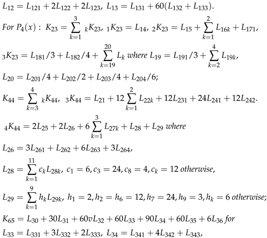
PROOF Since $q=1, {\sum }^N$ becomes N. We write $T_{1-s}^{1-r},U_{1-s}^{1-r},V_{1-s}^{1-r}$ as $T_{1-s}^r,U_{1-s}^r,V_{1-s}^r$. By Theorem 3.1 we need the following.

$$\begin{array}{cc}& T_{1-4}^3/3={\overline{t}}_{13}{\overline{t}}_2{\overline{t}}_4, T_{1-3}^2/2={\overline{t}}_{12}{\overline{t}}_3, T_{1-4}^2/2={\overline{t}}_{1-3}{\overline{t}}_4+{\overline{t}}_{13}{\overline{t}}_{24},\hfill \\ & T_{1-5}^4/12={\overline{t}}_{14}{\overline{t}}_2{\overline{t}}_3{\overline{t}}_5, T_{1-6}^4/4={\overline{t}}_{135}{\overline{t}}_2{\overline{t}}_4{\overline{t}}_6+3{\overline{t}}_{13}{\overline{t}}_{25}{\overline{t}}_4{\overline{t}}_6,\hfill \\ & T_{1-5}^3/3={\overline{t}}_{124}{\overline{t}}_3{\overline{t}}_5+3{\overline{t}}_{145}{\overline{t}}_2{\overline{t}}_3/2+3{\overline{t}}_{12}{\overline{t}}_{34}{\overline{t}}_5+3{\overline{t}}_{14}{\overline{t}}_{25}{\overline{t}}_3,\hfill \\ & T_{1-6}^3=3{\overline{t}}_{1235}{\overline{t}}_4{\overline{t}}_6/2+6{\overline{t}}_{1-3}{\overline{t}}_{45}{\overline{t}}_6+3{\overline{t}}_{135}{\overline{t}}_{24}{\overline{t}}_6+{\overline{t}}_{13}{\overline{t}}_{25}{\overline{t}}_{46},\hfill \\ & T_{1-6}^5/20={\overline{t}}_{15}{\overline{t}}_2{\overline{t}}_3{\overline{t}}_4{\overline{t}}_6, U_{1-6}^5/15={\overline{t}}_{14}{\overline{t}}_2{\overline{t}}_3{\overline{t}}_5{\overline{t}}_6,\hfill \\ & T_{1-7}^5/30={\overline{t}}_{146}{\overline{t}}_2{\overline{t}}_3{\overline{t}}_5{\overline{t}}_7+2{\overline{t}}_{14}{\overline{t}}_{26}{\overline{t}}_3{\overline{t}}_5{\overline{t}}_7+2{\overline{t}}_{14}{\overline{t}}_{56}{\overline{t}}_2{\overline{t}}_3{\overline{t}}_7,\hfill \\ & T_{1-8}^5={\overline{t}}_{1357}{\overline{t}}_2{\overline{t}}_4{\overline{t}}_6{\overline{t}}_8+60{\overline{t}}_{135}{\overline{t}}_{27}{\overline{t}}_4{\overline{t}}_6{\overline{t}}_8+60{\overline{t}}_{13}{\overline{t}}_{25}{\overline{t}}_{47}{\overline{t}}_6{\overline{t}}_8. U_{1-4}^2={\overline{t}}_{1-3}{\overline{t}}_4/3+{\overline{t}}_{12}{\overline{t}}_{34}/4,\hfill \\ & T_{1-5}^2={\overline{t}}_{1-4}{\overline{t}}_5/3+{\overline{t}}_{1245}{\overline{t}}_3/2+{\overline{t}}_{124}{\overline{t}}_{35}+{\overline{t}}_{145}{\overline{t}}_{23}/2,\hfill \\ & T_{1-6}^2={\overline{t}}_{1-5}{\overline{t}}_6+2{\overline{t}}_{1235}{\overline{t}}_{46}+{\overline{t}}_{1-3}{\overline{t}}_{4-6}+2{\overline{t}}_{135}{\overline{t}}_{246}/3,\hfill \\ & T_{1-5}^4/12={\overline{t}}_{14}{\overline{t}}_2{\overline{t}}_3{\overline{t}}_5, U_{1-5}^4/4={\overline{t}}_{12}{\overline{t}}_3{\overline{t}}_4{\overline{t}}_5,\hfill \\ & U_{1-6}^4/2=3{\overline{t}}_{125}{\overline{t}}_3{\overline{t}}_4{\overline{t}}_6+2{\overline{t}}_{156}{\overline{t}}_2{\overline{t}}_3{\overline{t}}_4+6{\overline{t}}_{12}{\overline{t}}_{35}{\overline{t}}_4{\overline{t}}_6+3{\overline{t}}_{15}{\overline{t}}_{26}{\overline{t}}_3{\overline{t}}_4,\hfill \\ & V_{1-6}^4/6={\overline{t}}_{124}{\overline{t}}_3{\overline{t}}_5{\overline{t}}_6+{\overline{t}}_{12}{\overline{t}}_{34}{\overline{t}}_5{\overline{t}}_6+{\overline{t}}_{14}{\overline{t}}_{25}{\overline{t}}_3{\overline{t}}_6,\hfill \\ & T_{1-7}^4=6{\overline{t}}_{1246}{\overline{t}}_3{\overline{t}}_5{\overline{t}}_7+3{\overline{t}}_{1456}{\overline{t}}_2{\overline{t}}_3{\overline{t}}_7+24{\overline{t}}_{124}{\overline{t}}_{36}{\overline{t}}_5{\overline{t}}_7+12{\overline{t}}_{124}{\overline{t}}_{56}{\overline{t}}_3{\overline{t}}_7\hfill \\ & +12{\overline{t}}_{145}{\overline{t}}_{26}{\overline{t}}_3{\overline{t}}_7+12{\overline{t}}_{146}{\overline{t}}_{23}{\overline{t}}_5{\overline{t}}_7+24{\overline{t}}_{146}{\overline{t}}_{25}{\overline{t}}_3{\overline{t}}_7+4{\overline{t}}_{146}{\overline{t}}_{57}{\overline{t}}_2{\overline{t}}_3\hfill \\ & +12{\overline{t}}_{456}{\overline{t}}_{17}{\overline{t}}_2{\overline{t}}_3+12{\overline{t}}_{12}{\overline{t}}_{34}{\overline{t}}_{56}{\overline{t}}_7+12{\overline{t}}_{14}{\overline{t}}_{25}{\overline{t}}_{36}{\overline{t}}_7+12{\overline{t}}_{14}{\overline{t}}_{26}{\overline{t}}_{57}{\overline{t}}_3,\hfill \\ & T_{1-8}^4=2{\overline{t}}_{12357}{\overline{t}}_4{\overline{t}}_6{\overline{t}}_8+12{\overline{t}}_{1235}{\overline{t}}_{47}{\overline{t}}_6{\overline{t}}_8+6{\overline{t}}_{1357}{\overline{t}}_{24}{\overline{t}}_6{\overline{t}}_8\hfill \\ & +6{\overline{t}}_{123}{\overline{t}}_{457}{\overline{t}}_6{\overline{t}}_8+6{\overline{t}}_{135}{\overline{t}}_{247}{\overline{t}}_6{\overline{t}}_8+12{\overline{t}}_{123}{\overline{t}}_{45}{\overline{t}}_{67}{\overline{t}}_8+24{\overline{t}}_{135}{\overline{t}}_{24}{\overline{t}}_{67}{\overline{t}}_8\hfill \\ & +6{\overline{t}}_{135}{\overline{t}}_{27}{\overline{t}}_{48}{\overline{t}}_6+3{\overline{t}}_{13}{\overline{t}}_{25}{\overline{t}}_{47}{\overline{t}}_{68}, T_{1-7}^6/30={\overline{t}}_{16}{\overline{t}}_2{\overline{t}}_3{\overline{t}}_4{\overline{t}}_5{\overline{t}}_7, U_{1-7}^6/60={\overline{t}}_{15}{\overline{t}}_2{\overline{t}}_3{\overline{t}}_4{\overline{t}}_6{\overline{t}}_7,\hfill \end{array}$$

$$\begin{array}{cc}& T_{1-8}^6/60={\overline{t}}_{157}{\overline{t}}_2{\overline{t}}_3{\overline{t}}_4{\overline{t}}_6{\overline{t}}_8+3{\overline{t}}_{15}{\overline{t}}_{27}{\overline{t}}_3{\overline{t}}_4{\overline{t}}_6{\overline{t}}_8+2{\overline{t}}_{15}{\overline{t}}_{67}{\overline{t}}_2{\overline{t}}_3{\overline{t}}_4{\overline{t}}_8,\hfill \\ & U_{1-8}^6/90={\overline{t}}_{147}{\overline{t}}_2{\overline{t}}_3{\overline{t}}_5{\overline{t}}_6{\overline{t}}_8+4{\overline{t}}_{14}{\overline{t}}_{27}{\overline{t}}_3{\overline{t}}_5{\overline{t}}_6{\overline{t}}_8+{\overline{t}}_{17}{\overline{t}}_{48}{\overline{t}}_2{\overline{t}}_3{\overline{t}}_5{\overline{t}}_6,\hfill \\ & T_{1-9}^6/60={\overline{t}}_{1468}{\overline{t}}_2{\overline{t}}_3{\overline{t}}_5{\overline{t}}_7{\overline{t}}_9+6{\overline{t}}_{146}{\overline{t}}_{28}{\overline{t}}_3{\overline{t}}_5{\overline{t}}_7{\overline{t}}_9+6{\overline{t}}_{146}{\overline{t}}_{58}{\overline{t}}_2{\overline{t}}_3{\overline{t}}_7{\overline{t}}_9\hfill \\ & +3{\overline{t}}_{468}{\overline{t}}_{15}{\overline{t}}_2{\overline{t}}_3{\overline{t}}_7{\overline{t}}_9+2{\overline{t}}_{14}{\overline{t}}_{26}{\overline{t}}_{38}{\overline{t}}_5{\overline{t}}_7{\overline{t}}_9+12{\overline{t}}_{14}{\overline{t}}_{26}{\overline{t}}_{58}{\overline{t}}_3{\overline{t}}_7{\overline{t}}_9+6{\overline{t}}_{14}{\overline{t}}_{56}{\overline{t}}_{78}{\overline{t}}_2{\overline{t}}_3{\overline{t}}_9,\hfill \\ & T_{1-10}^6/6={\overline{t}}_{13579}{\overline{t}}_2{\overline{t}}_4{\overline{t}}_6{\overline{t}}_8{\overline{t}}_{10}+20{\overline{t}}_{1357}{\overline{t}}_{29}{\overline{t}}_4{\overline{t}}_6{\overline{t}}_8{\overline{t}}_{10}\hfill \\ & +15{\overline{t}}_{135}{\overline{t}}_{279}{\overline{t}}_4{\overline{t}}_6{\overline{t}}_8{\overline{t}}_{10}+60{\overline{t}}_{135}{\overline{t}}_{27}{\overline{t}}_{49}{\overline{t}}_6{\overline{t}}_8{\overline{t}}_{10}+60{\overline{t}}_{135}{\overline{t}}_{27}{\overline{t}}_{89}{\overline{t}}_4{\overline{t}}_6{\overline{t}}_{10}+60{\overline{t}}_{13}{\overline{t}}_{25}{\overline{t}}_{47}{\overline{t}}_{69}{\overline{t}}_8{\overline{t}}_{10}.\hfill \\ & For{P}_1\left(x\right): T_{1-4}^3 {\overline{k}}_1^{12}{\overline{k}}_1^{34}=3c_{23}.\hfill \\ & For{P}_2\left(x\right): T_{1-3}^2 {\overline{k}}_2^{1-3}/2=c_{15}, T_{1-4}^2 {\overline{k}}_1^{12}{\overline{k}}_1^{34}/2=c_{19}/2+c_{1,10};\hfill \\ & K_{43}=c_{31}+g_1+g_{2}for{g}_1=T_{1-5}^4 {\overline{k}}_2^{1-3}{\overline{k}}_1^{45}=12c_{36},\hfill \\ & g_2=T_{1-6}^4 {\overline{k}}_1^{12}{\overline{k}}_1^{34}{\overline{k}}_1^{56}=4c_{3,11}+12c_{3,10}.\hfill \\ & For{P}_3\left(x\right):{ }_2{K}_{33}=L_4+3L_5^{\prime }, L_5^{\prime }=T_{1-4}^3/3 {\left({\overline{k}}^{12}{\overline{k}}^{34}\right)}_3={\overline{t}}_{13}{\overline{t}}_2{\overline{t}}_4 {\left({\overline{k}}^{12}{\overline{k}}^{34}\right)}_3=2L_5,\hfill \\ & L_6=T_{1-4}^3/3 {\overline{k}}_3^{1-4}, L_7=T_{1-5}^3/3 {\overline{k}}_2^{1-3}{\overline{k}}_1^{45},\hfill \\ & L_{71}={\overline{s}}^4{\overline{t}}_{412} {\overline{k}}_2^{1-3}{\overline{t}}_3, L_8=T_{1-6}^3 {\overline{k}}_1^{12}{\overline{k}}_1^{34}{\overline{k}}_1^{56},\hfill \\ & L_{81}={\overline{t}}_{1235}{\overline{t}}_4{\overline{t}}_6 {\overline{k}}_1^{12}{\overline{k}}_1^{34}{\overline{k}}_1^{56}, L_{82}={\overline{t}}_{1-3}{\overline{t}}_{45}{\overline{t}}_6 {\overline{k}}_1^{12}{\overline{k}}_1^{34}{\overline{k}}_1^{56}, L_{83}={\overline{t}}_{135}{\overline{t}}_{24}{\overline{t}}_6 {\overline{k}}_1^{12}{\overline{k}}_1^{34}{\overline{k}}_1^{56},\hfill \\ & L_{84}={\overline{t}}_{13}{\overline{t}}_{25}{\overline{t}}_{46} {\overline{k}}_1^{12}{\overline{k}}_1^{34}{\overline{k}}_1^{56}.\hfill \\ & K_{54}isgivenby\left(\right)with{L}_{10}=T_{1-6}^5/20 {\overline{k}}_3^{1-4}{\overline{k}}_1^{56}, L_{11}=U_{1-6}^5/15 {\overline{k}}_2^{1-3}{\overline{k}}_2^{4-6},\hfill \\ & L_{12}=T_{1-7}^5/30 {\overline{k}}_2^{1-3}{\overline{k}}_1^{45}{\overline{k}}_1^{67}, L_{121}={\overline{t}}_2{\overline{t}}_3{\overline{k}}_2^{1-3}{\overline{t}}_{146}{\overline{s}}^4{\overline{s}}^6, L_{13}=T_{1-8}^5 {\overline{k}}_1^{12}{\overline{k}}_1^{34}{\overline{k}}_1^{56}{\overline{k}}_1^{78}.\hfill \\ & For{P}_4\left(x\right):{ }_2{K}_{23}=L_{15}+L_{16}+L_{17}/2, L_{15}=T_{1-3}^2/2 {\overline{k}}_3^{1-3}, L_{16}=\sum _{k=1}^2{L}_{16k},\hfill \\ & L_{162}={\overline{s}}^2{\overline{t}}_{2-4}{\overline{k}}_2^{34}, L_{17}=T_{1-4}^2/2 {\left({\overline{k}}^{12}{\overline{k}}^{34}\right)}_3=\sum _{k=1}^2{L}_{17k}, L_{172}=L_{171};\hfill \\ & { }_3{K}_{23}=\sum _{k=18}^{20}{L}_k: L_{18}=U_{1-4}^2{\overline{k}}_3^{1-4}=L_{181}/3+L_{182}/4,\hfill \\ & L_{19}=T_{1-5}^2{\overline{k}}_2^{1-3}{\overline{k}}_1^{45}=\sum _{k=1}^4{L}_{19k}/g_{k}for{g}_1=3,g_2=g_3=g_4=1,\hfill \\ & L_{192}={\overline{t}}_3{\overline{k}}_2^{1-3}{\overline{t}}_{1245}{\overline{k}}_1^{45}, L_{193}={\overline{t}}_{412}{\overline{k}}_2^{1-3}{\overline{t}}_{35}{\overline{k}}_1^{54}, L_{194}={\overline{k}}_1^{45}{\overline{t}}_{451}{\overline{k}}_2^{1-3}{\overline{t}}_{23},\hfill \\ & L_{20}=T_{1-6}^2{\overline{k}}_1^{12}{\overline{k}}_1^{34}{\overline{k}}_1^{56}/4=L_{201}/4+L_{202}/2+L_{203}/4+L_{204}/6,\hfill \\ & L_{202}={\overline{k}}_1^{12}{\overline{t}}_{1235} \left({\overline{k}}_1^{34}{\overline{k}}_1^{56}\right) {\overline{t}}_{46}.\hfill \\ & { }_3{K}_{44}=L_{21}+12L_{22}+4L, L=T_{1-6}^4/4 {\left({\overline{k}}^{12}{\overline{k}}^{34}{\overline{k}}^{56}\right)}_4=L_{23}+3L_{24},\hfill \\ & L_{22}=T_{1-5}^4/12 {\left({\overline{k}}^{1-3}{\overline{k}}^{45}\right)}_4=(L_{221}+L_{222})by\left(\right),\hfill \end{array}$$

$$\begin{array}{cc}& L_{23}={\overline{t}}_{135}{\overline{t}}_2{\overline{t}}_4{\overline{t}}_6 {\left({\overline{k}}^{12}{\overline{k}}^{34}{\overline{k}}^{56}\right)}_4=\sum _{k=1}^3{L}_{23k}by\left(\right), L_{23k}\equiv L_{231}.By\left(\right),\hfill \\ & L_{24}={\overline{t}}_{13}{\overline{t}}_{25}{\overline{t}}_4{\overline{t}}_6 {\left({\overline{k}}^{12}{\overline{k}}^{34}{\overline{k}}^{56}\right)}_4=2L_{241}+L_{242};\hfill \\ & { }_4{K}_{44}=2L_{25}+2L_{26}+6L_{27}+L_{28}+L_{29}, L_{25}={\overline{k}}_4^{1-5}{U}_{1-5}^4/4,\hfill \\ & L_{26}=U_{1-6}^4/2 {\overline{k}}_3^{1-4}{\overline{k}}_1^{56}, L_{27}=V_{1-6}^4/6 {\overline{k}}_2^{1-3}{\overline{k}}_2^{4-6}=\sum _{k=1}^3{L}_{27k},\hfill \\ & L_{28}=T_{1-7}^4{\overline{k}}_2^{1-3}{\overline{k}}_1^{45}{\overline{k}}_1^{67}, L_{29}=T_{1-8}^4{\overline{k}}_1^{12}{\overline{k}}_1^{34}{\overline{k}}_1^{56}{\overline{k}}_1^{78};\hfill \\ & for{K}_{65}: L_{31}=T_{1-7}^6/30 k_4^{1-5}{k}_1^{67},\hfill \\ & L_{32}=U_{1-7}^6/60 k_4^{1-5}{k}_1^{67}/v, L_{33}=T_{1-8}^6/60 {\overline{k}}_3^{1-4}{\overline{k}}_1^{56}{\overline{k}}_1^{78}, L_{34}=U_{1-8}^6/90 {\overline{k}}_2^{1-3}{\overline{k}}_2^{4-6}{\overline{k}}_2^{78},\hfill \\ & L_{35}=T_{1-9}^6/60 {\overline{k}}_2^{1-3}{\overline{k}}_1^{45}{\overline{k}}_1^{67}{\overline{k}}_1^{89}, L_{36}=T_{1-10}^6/6 {\overline{k}}_1^{12}{\overline{k}}_1^{34}{\overline{k}}_1^{56}{\overline{k}}_1^{78}{\overline{k}}_1^{9,10}. \square \hfill \end{array}$$

Example 1. 

Suppose that $E \widehat{w}=w$ and $t\left(w\right)$ is linear in w. Then $K_{1e}=0$ for $e\ge 1$. For $r\le 4$, the $K_{ij}$ needed for $P_r\left(x\right)$ of () for the distribution of $Y_{nt}$ of (5) are as follows.

$$\begin{array}{cc}& K_{10}=\overline{t}=t\left(w\right). For{P}_0\left(x\right): K_{21}=v. For{P}_1\left(x\right): K_{32}=c_{21}.\hfill \\ & For{P}_2\left(x\right): K_{22}={ }_1{K}_{22}=c_{11}, K_{43}=c_{31}.\hfill \\ & For{P}_3\left(x\right): K_{33}={ }_2{K}_{33}=L_4, K_{54}=L_9.\hfill \\ & For{P}_4\left(x\right): K_{23}={ }_1{K}_{23}=L_{14}, K_{44}={ }_3{K}_{44}=L_{21}, K_{65}=L_{30}.\hfill \end{array}$$

For, ${\overline{u}}_1,{\overline{v}}^1,{\overline{x}}_1,{\overline{z}}_{12}$ are 0, as are most $c_{ij},L_k$ and ${ }_2{K}_{22},{ }_3{K}_{33},{ }_2{K}_{23},{ }_3{K}_{23},{ }_4{K}_{44}.$ So for $r=0,\cdots ,4$, for $P_r\left(x\right)$ we only need to calculate these 3 $c_{ij}$ and 5 $L_j$.

Let $G_{\gamma }$ be a gamma random variable with known mean $\gamma .$ Its rth cumulant is $(r-1)!\gamma .$

Example 2. 

Linear combinations of scale parameters.Suppose that $E \widehat{w}=w$ and $t\left(w\right)$ is linear, the components of $\widehat{w}$ are independent, and for $1\le i\le p, {\widehat{w}}^i/w^i$ has a distribution with known rth cumulant $n^{1-r}{\kappa }_{ri}$. Then $K_{re}=0$ for $e\ne r-1$ and

$$K_{r,r-1}=\sum _{i=1}^p{t}_{\cdot i}^r{\kappa }_{ri}{\left(w^i\right)}^r.$$

For example if ${\widehat{w}}_i/w_i$ is a standard exponential variable then ${\kappa }_{ri}=(r-1)!$.

For $s\le r$ and any function $f^{i_s\cdots i_r}$, set ${\sum }_{s-r}{\overline{f}}^{s-r}={\sum }_{i_s,\cdots ,i_r}{f}^{i_s\cdots i_r}$ summed over their range. In Example 5.3 their range is $1,2$; for example in $L_{123},$ ${\sum }_1{t}_{\cdot 2i_1}{\overline{v}}^1={\sum }_{i_1=1}^k{t}_{\cdot 2i_1}{\overline{v}}^1.$ In Example 5.4 their range is $1,\cdots ,k$; for example ${\overline{u}}_1={\sum }_2{\overline{t}}_{12}{\overline{s}}^2={\sum }_{i_2=1}^k{\overline{t}}_{12}{\overline{s}}^2.$

Example 3. 

Suppose that $\widehat{\mu }\sim {\mathcal{N}}_1(\mu ,V/n)$ and $\widehat{V}/V={\chi }_f^2/f=G_{\gamma }/\gamma$ are independent, where $\gamma =f/2$ has magnitude n. Set $\nu =\gamma /n$. Then

${\kappa }_r\left(\widehat{\mu }\right)=\mu {\delta }_{r1}+V{n}^{-1}{\delta }_{r2},{\kappa }_r\left(\widehat{V}\right)=k_r{n}^{1-r}$ for $k_r=(r-1)!{\nu }^{1-r}{V}^r$, and cross-cumulants of $\widehat{w}$ are zero. Take $p=2, w_1=\mu , w_2=V$. Then by Corollary 5.1, $K_{re}$ are given in terms of

$$\begin{array}{cc}\hfill s^1& =t_{\cdot 1}V, s^2=t_{\cdot 2}{k}_2, u_1=t_{\cdot 11}{t}_{\cdot 1}V+t_{\cdot 12}{t}_{\cdot 2}{k}_2, u_2=t_{\cdot 12}{t}_{\cdot 1}V+t_{\cdot 22}{t}_{\cdot 2}{k}_2,\hfill \\ \hfill v^1& =V{u}_1, v^2=k_2{u}_2,\hfill \end{array}$$

as follows.

$$\begin{array}{cc}& For{P}_0\left(x\right): K_{21}=v=t_{\cdot 1}^{2}V+t_{\cdot 2}^2{k}_2/2.\hfill \\ & For{P}_1\left(x\right): c_{02}=t_{\cdot 11}+t_{\cdot 22}{k}_2, c_{21}=t_{\cdot 2}^3{k}_3, c_{23}=\sum _{i=1}^2{t}_{\cdot ii}{\left(s^i\right)}^2.\hfill \\ & For{P}_2\left(x\right): c_{11}=0, c_{15}=t_{\cdot 22}{t}_{\cdot 2}{k}_3, c_{19}={\left(t_{\cdot 11}V\right)}^1+{\left(t_{\cdot 22}{k}_2\right)}^2+2t_{\cdot 12}V{k}_2,\hfill \\ & c_{31}=t_{\cdot 2}^4{k}_4, c_{36}=t_{\cdot 2}^2{k}_3{u}_2, c_{3,10}=u_1^{2}V+u_2^2 k_2,\hfill \\ & c_{3,11}=\sum _{i=1}^2{\left(s^i\right)}^3{t}_{\cdot iii}+3\sum _{12}^2{\left(s^1\right)}^2{s}^2{t}_{\cdot 112}where\sum _{12}^2{f}_{12}=f_{12}+f_{21}.\hfill \\ & For{P}_3\left(x\right): L_1=L_4=L_5=0, L_2=t_{\cdot 222}{k}_3,\hfill \\ & L_3=t_{\cdot 1111}{V}^2+2t_{\cdot 1122}V{k}_2+t_{\cdot 2222}{k}_2^2,\hfill \\ & L_6=t_{\cdot 22}{t}_{\cdot 2}^2{k}_4, L_{71}=z_{22}{k}_3{t}_2, L_{72}=y^2(t_{\cdot 211}V+t_{\cdot 222}{k}_3), L_{73}=t_{\cdot 22}{k}_3{u}_2,\hfill \\ & L_{74}=(V{t}_{\cdot 12}^2+k_2{t}_{\cdot 22}^2)k_3{t}_{\cdot 2}, L_{81}=(V{t}_{\cdot 1i_2{i}_3{i}_4}+k_2{t}_{\cdot 2i_2{i}_3{i}_4}){\overline{s}}^3{\overline{s}}^4,\hfill \end{array}$$

$$\begin{array}{cc}& L_{82}=\sum _1(V{t}_{\cdot 11i_1}+k_2{t}_{\cdot 22i_1})v^{i_1}, L_{83}=V^2{t}_{\cdot 11}{z}_{11}+2V{k}_2{t}_{\cdot 12}{z}_{12}+k_2^2{t}_{\cdot 22}{z}_{22},\hfill \\ & L_{84}=\sum _{1-3}{\overline{k}}_1^{11}{\overline{k}}_1^{22}{\overline{k}}_1^{33}{\overline{t}}_{12}{\overline{t}}_{23}{\overline{t}}_{31},\hfill \\ & L_9=t_{\cdot 2}^5{k}_5, L_{10}=u_2{t}_{\cdot 2}^3{k}_4, L_{11}={\left(y^2\right)}^2{t}_{\cdot 22}, L_{121}=y^2\sum _{12}{t}_{\cdot 2i_1{i}_2}{\overline{s}}^1{\overline{s}}^2,\hfill \\ & L_{122}=t_{\cdot 2}{k}_3{u}_2^2, L_{123}=y^2\sum _1{t}_{\cdot 2i_1}{\overline{v}}^1, L_{13}=\sum _{1-3}{\overline{s}}^1{\overline{s}}^2{\overline{t}}_{1-3}{\overline{k}}_1^{33}{\overline{u}}_3.\hfill \end{array}$$

Similarly one can write down the Ls needed for $P_4\left(x\right)$.

Example 4. 

Suppose that we have the summary statistics from k samples of size $n_i$ from normal populations with means and variances ${\mu }_i,V_i, 1\le i\le k$. Take $p=2k, w_i={\mu }_i, w_{i+k}=V_i, 1\le i\le k$. So we have p independent statistics, ${\widehat{\mu }}_i\sim \mathcal{N}({\mu }_i,V_i/n_i)$ and ${\widehat{V}}_i\sim V_i{\chi }_{f_i}^2/f_i=V_i{G}_{{\gamma }_i}/{\gamma }_i, 1\le i\le k$ where ${\gamma }_i=f_i/2$ has magnitude n, the total sample size. Set

$${\nu }_i={\gamma }_i/n, {\lambda }_i=n_i/n, {\tau }_i=V_i/{\lambda }_i.$$

Then ${\kappa }_r\left({\widehat{\mu }}_i\right)={\mu }_i{\delta }_{r1}+V_i{\left({\lambda }_{i}n\right)}^{-1}{\delta }_{r2},{\kappa }_r\left({\widehat{V}}_i\right)=k_{ri}{\left({\lambda }_{i}n\right)}^{1-r}$ for $k_{ri}=(r-1)!{\nu }_i^{1-r}$, and cross-cumulants of $\widehat{w}$ are zero. Suppose that $t\left(w\right)$ only depends on ${\mu }_1,\cdots ,{\mu }_k$, as in Example 3.3 of Withers (1982). (The notation there is slightly different.) Then

$${\overline{s}}^1={\overline{t}}_1{\overline{\tau }}_1, {\overline{u}}_1=\sum _2{\overline{t}}_{12}{\overline{s}}^2, {\overline{v}}^1={\overline{\tau }}_1{\overline{u}}_1, {\overline{z}}_{12}=\sum _3{\overline{t}}_{1-3}{\overline{s}}^3,$$

and by Corollary 5.1, the coefficients needed are as follows.

$$\begin{array}{cc}& For{P}_0\left(x\right): K_{21}=v={\overline{t}}_1{\overline{s}}^1=\sum _1{\overline{t}}_1^2{\overline{\tau }}_1,\hfill \\ & For{P}_1\left(x\right): c_{02}=\sum _1{\overline{t}}_{11}{\overline{\tau }}_1, c_{21}=0, c_{23}={\overline{s}}^1{\overline{t}}_{12}{\overline{s}}^2=\sum _{12}{\overline{t}}_1{\overline{\tau }}_1{\overline{t}}_{12}{\overline{t}}_2{\overline{\tau }}_2,\hfill \\ & For{P}_2\left(x\right), K_{22}: c_{11}=c_{15}=0, c_{19}=\sum _{12}{\overline{t}}_{12}^2{\overline{\tau }}_1{\overline{\tau }}_2,c_{1,10}=\sum _{12}{\overline{t}}_1{\overline{\tau }}_1{\overline{t}}_{122}{\overline{\tau }}_2;\hfill \\ & For{K}_{43}: c_{31}=c_{36}=0, c_{3,10}=\sum _1{\overline{u}}_1^2{\overline{\tau }}_1, c_{3,11}=\sum _{1-3}{\overline{s}}^1{\overline{s}}^2{\overline{s}}^3{\overline{t}}_{1-3}.\hfill \\ & For{P}_3\left(x\right), K_{12}=L_3/6=\sum _{12}{\overline{t}}_{1122}{\overline{\tau }}_1{\overline{\tau }}_2/6as{L}_1=L_2=0;\hfill \\ & for{K}_{33}: L_4=L_5=L_6=L_7=0, L_{81}=\sum _{1-3}{\overline{\tau }}_1{\overline{t}}_{1123}{\overline{s}}^2{\overline{s}}^3, L_{82}=\sum _{12}{\overline{\tau }}_1{\overline{t}}_{122}{\overline{v}}^2,\hfill \\ & L_{83}=\sum _{12}{\overline{t}}_{12}{\overline{\tau }}_1{\overline{\tau }}_2{\overline{z}}_{12}=\sum _{1-3}{\overline{\tau }}_1{\overline{\tau }}_2{\overline{\tau }}_3{\overline{t}}_{12}{\overline{t}}_{123}{\overline{t}}_3, L_{83}=\sum _{1-3}{\overline{\tau }}_1{\overline{\tau }}_2{\overline{\tau }}_3{\overline{t}}_{12}{\overline{t}}_{23}{\overline{t}}_{31};\hfill \\ & for{K}_{54}: L_k=0for10\le k\le 14.\hfill \\ & For{P}_4\left(x\right), K_{23}: L_{i,k}=0fori=15,16,18,19, L_{171}=\sum _{12}{\overline{t}}_{12}^2{\overline{\tau }}_1{\overline{\tau }}_2,\hfill \\ & L_{201}=\sum _{1-3}{\overline{\tau }}_1{\overline{\tau }}_2{\overline{t}}_{11223}{\overline{s}}^5, L_{202}=\sum _{1-3}{\overline{\tau }}_1{\overline{\tau }}_2{\overline{\tau }}_3{\overline{t}}_{1123}{\overline{t}}_{23}, L_{203}=\sum _{1-3}{\overline{\tau }}_1{\overline{\tau }}_2{\overline{\tau }}_3{\overline{t}}_{112}{\overline{t}}_{233},\hfill \\ & L_{204}=\sum _{1-3}{\overline{\tau }}_1{\overline{\tau }}_2{\overline{\tau }}_3{\overline{t}}_{123}^2;\hfill \end{array}$$

$$\begin{array}{cc}& K_{44}=L_{29}as{L}_k=0fork=21,(22,k),(23,1),(24,k),25,(26,k),(27,k),(28,k),\hfill \\ & L_{291}=\sum _{1-4}{\overline{\tau }}_1{\overline{s}}^2{\overline{s}}^3{\overline{s}}^4{\overline{t}}_{11234}, L_{292}=\sum _{1-3}{\overline{\tau }}_1{\overline{t}}_{1123}{\overline{v}}^2{\overline{s}}^3, L_{293}=\sum _{1-4}{\overline{\tau }}_1{\overline{\tau }}_2{\overline{s}}^3{\overline{s}}^4{\overline{t}}_{1234},\hfill \\ & L_{294}=\sum _{1-4}{\overline{\tau }}_1{\overline{\tau }}_2{\overline{t}}_{112}{\overline{t}}_{234}{\overline{s}}^3{\overline{s}}^4, L_{295}=\sum _{12}{\overline{\tau }}_1{\overline{z}}_{12}^2{\overline{\tau }}_2, L_{296}=\sum _{1-3}{\overline{\tau }}_1{\overline{\tau }}_2{\overline{\tau }}_3{\overline{t}}_{112}{\overline{t}}_{23},\hfill \\ & L_{297}=\sum _{12}{\overline{\tau }}_1{\overline{x}}_{12}{\overline{t}}_{12}for{\overline{x}}_{12}=\sum _3{\overline{t}}_{123}{\overline{v}}^3, L_{298}=\sum _{1-3}{\overline{\tau }}_1{\overline{\tau }}_2{\overline{\tau }}_3{\overline{t}}_{12}{\overline{t}}_{23}{\overline{z}}_{31},\hfill \\ & L_{299}=\sum _{1-4}{\overline{\tau }}_1{\overline{\tau }}_2{\overline{\tau }}_3{\overline{\tau }}_4{\overline{t}}_{12}{\overline{t}}_{23}{\overline{t}}_{34}{\overline{t}}_{41};\hfill \\ & K_{65}=6L_{36},astheothercomponentsof{K}_{65}are0.Also,\hfill \\ & K_{13}=\sum _{1-3}{\overline{\tau }}_1{\overline{\tau }}_2{\overline{\tau }}_3{\overline{t}}_{112233}/48, K_{14}=\sum _{1-4}{\overline{\tau }}_1{\overline{\tau }}_2{\overline{\tau }}_3{\overline{\tau }}_4{\overline{t}}_{11223344}/384.\hfill \end{array}$$

Corollary 2. 

Set $Y_n=v^{-1/2}{Y}_{nt}={(n/v)}^{1/2}(t\left(\widehat{w}\right)-t\left(w\right)).$ Then

$$\begin{array}{c}\hfill Prob.(Y_n\le x)=\sum _{r=0}^{\infty }{n}^{-r/2}{P}_{rv}\left(x\right)\end{array}$$

where $P_{rv}\left(x\right)$ is $P_r\left(x\right)$ of Corollary 5.1 with $K_{re}$ replaced by $K_{re}/v^{r/2}.$

PROOF This is straightforward. □

Looking at $K_{re},c_{ab},v,{\overline{s}}^2,{\overline{u}}_3$ as functions of w, we denote their partial derivatives with respect to ${\overline{w}}_3=w_{i_3}$, say. by ${\overline{K}}_{re\cdot 3},{\overline{c}}_{ab\cdot 3},{\overline{v}}_{\cdot 3},{\overline{s}}_{\cdot 3}^2,{\overline{u}}_{3\cdot 3}$ and similarly for higher derivatives. We shall give the ones we need in Lemma 5.1. When constructing confidence regions, one needs to assume that the distribution of $\widehat{w}$ is determined by w. So far we’ve not assumed this. For $\widehat{w}$ biased, we need

Corollary 3. 

Let $\widehat{w}\in R^p$ be abiasedstandard estimate of w satisfying (1) where ${\overline{k}}_e^{1-r}$ may depend on w. Then for $q=1$, $\widehat{t}=t\left(\widehat{w}\right)$ is a standard estimate of $t=t\left(w\right)\in R$:

$$\begin{array}{cc}& {\kappa }_r\left(\widehat{t}\right)=\sum _{e=r-1}^{\infty }{n}^{-e}{a}_{re}forr\ge 1,where{a}_{re}=K_{re}+D_{re}, D_{r,r-1}=0,\hfill \end{array}$$

(6)

and the other $D_{re}$ needed for $P_j\left(x\right)$ of () for the distribution of $Y_{nt}$ of (5) are as follows.

$$\begin{array}{cc}& For{P}_0\left(x\right): D_{21}=0\Rightarrow a_{21}=K_{21}=v={\overline{t}}_1{\overline{k}}_1^{12}{\overline{t}}_2.\hfill \\ & For{P}_1\left(x\right):D_{11}=c_{01}\Rightarrow a_{11}=c_{01}+c_{02}/2, a_{32}=K_{32}=c_{21}+3c_{23},\hfill \end{array}$$

$$\begin{array}{cc}& For{P}_2\left(x\right): D_{22}={\overline{v}}_{\cdot 3} {\overline{k}}_1^3=c_{12}+2c_{16}, a_{43}=K_{43}.\hfill \\ & For{P}_3\left(x\right): D_{12}=K_{11,1}+K_{10,2}, K_{11,1}={\overline{K}}_{11\cdot 3} {\overline{k}}_1^3, K_{10,2}={\overline{t}}_1{\overline{k}}_2^1+{\overline{k}}_1^1{\overline{t}}_{12}{\overline{k}}_1^2/2,\hfill \\ & D_{33}={\overline{K}}_{32\cdot 4} {\overline{k}}_1^4, a_{54}=K_{54}.\hfill \\ & For{P}_4\left(x\right): D_{23}=K_{22,1}+K_{21,2}, K_{22,1}={\overline{K}}_{22\cdot 3} {\overline{k}}_1^3, K_{21,2}={\overline{v}}_{\cdot 3} {\overline{k}}_2^3/2+{\overline{v}}_{\cdot 34} {\overline{k}}_1^3{\overline{k}}_1^4,\hfill \\ & D_{44}={\overline{K}}_{43\cdot 5} {\overline{k}}_1^5, a_{65}=K_{65}.\hfill \end{array}$$

PROOF This follows from Theorem 4.1. $D_{rc}={\sum }_{c=1}^{c-r+1}{K}_{r,c-r,e}$ where $K_{rke}$ is the coefficient of $n^{-e}$ in the expansion of $K_{rk}(E \widehat{w})$ about $K_{rk}$. □

For $r\le s$, and any ${\overline{X}}_{r-s}$, let ${\sum }_{r-s}^N{\overline{X}}_{r-s}$ sums over all N permutations of $i_r,\cdots ,i_s$ giving distinct terms. For example

$$\sum _{3-5}^3{\overline{t}}_{13}{\overline{t}}_{245}={\overline{t}}_{13}{\overline{t}}_{245}+{\overline{t}}_{14}{\overline{t}}_{235}+{\overline{t}}_{15}{\overline{t}}_{234}.$$

The derivatives of $v=K_{21}$ and $K_{re}$ needed for Corollary 5.3 are given by by

Lemma 1. 

$$\begin{array}{cc}& {\overline{v}}_{\cdot 3}=2{\overline{u}}_3+{\overline{T}}_3, {\overline{v}}_{\cdot 34}=\sum _{k=0}^2{\overline{v}}_{34k},where{\overline{T}}_3={\overline{t}}_1{\overline{t}}_2{\overline{k}}_{1\cdot 3}^{12},\hfill \\ & {\overline{v}}_{340}=2{\overline{z}}_{34}+2{\overline{t}}_{31}{\overline{k}}_1^{12}{\overline{t}}_{24}, {\overline{v}}_{341}=2{\overline{t}}_1({\overline{k}}_{1\cdot 3}^{12}{\overline{t}}_{24}+{\overline{k}}_{1\cdot 4}^{12}{\overline{t}}_{23}), {\overline{v}}_{342}={\overline{t}}_1{\overline{t}}_2{\overline{k}}_{1\cdot 34}^{12}.\hfill \end{array}$$

(7)

(8)

$$\begin{array}{cc}& {\overline{K}}_{43\cdot 5}=c_{31\cdot 5}+12c_{36\cdot 5}+12c_{3,10\cdot 5}+4c_{3,11\cdot 5}for{c}_{31\cdot 5}=4{\overline{t}}_{51} {\overline{k}}_3^{1-4}{\overline{t}}_2{\overline{t}}_3{\overline{t}}_4\hfill \\ & +{\overline{t}}_1\cdots {\overline{t}}_4 {\overline{k}}_{3\cdot 5}^{1-4}, c_{36\cdot 5}=2{\overline{t}}_{51}{\overline{k}}_2^{1-3}{\overline{t}}_2{\overline{u}}_3+{\overline{t}}_1{\overline{t}}_2{\overline{u}}_3{\overline{k}}_{2\cdot 5}^{1-3}+{\overline{y}}^3{\overline{t}}_{3-5}{\overline{s}}^4+{\overline{Y}}_4({\overline{k}}_{1\cdot 5}^{41}{\overline{t}}_1+{\overline{k}}_1^{41}{\overline{t}}_{15}).\hfill \\ & c_{3,10\cdot 3}={\overline{u}}_1{\overline{k}}_{1\cdot 3}^{12}{\overline{u}}_2+2{\overline{v}}^1{\overline{s}}^2{\overline{t}}_{1-3}+2{\overline{t}}_1{\overline{x}}_2{\overline{k}}_{1\cdot 3}^{12}+2{\overline{x}}_1{\overline{k}}_1^{12}{\overline{t}}_{23}, \hfill \\ & c_{3,11\cdot 5}=3{\overline{s}}^1{\overline{s}}^2{\overline{t}}_{1-3}{\overline{s}}_{\cdot 5}^3=3{\overline{s}}^1{\overline{s}}^2{\overline{t}}_{1-3}{\overline{t}}_4{\overline{k}}_{1\cdot 5}^{34}+3{\overline{s}}^1{\overline{s}}^2{\overline{t}}_{1-3}{\overline{k}}_1^{34}{\overline{t}}_{45}.\hfill \end{array}$$

(9)

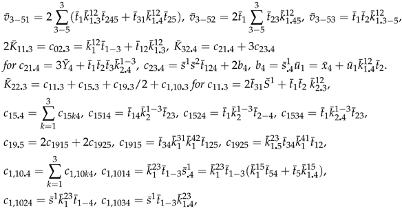
PROOF For example substitute ${\overline{u}}_{3\cdot 5}={\overline{t}}_{3-5}{\overline{s}}^4+{\overline{t}}_{34}{\overline{k}}_{1\cdot 5}^{41}{\overline{t}}_1+{\overline{t}}_{34}{\overline{k}}_1^{41}{\overline{t}}_{15}$ into

$c_{36\cdot 5}=2{\overline{t}}_1{\overline{t}}_{25}{\overline{k}}_2^{1-3}{\overline{u}}_3+{\overline{t}}_1{\overline{t}}_2({\overline{k}}_{2\cdot 5}^{1-3}{\overline{u}}_3+{\overline{k}}_2^{1-3}{\overline{u}}_{3\cdot 5}).$□

So now we can write $D_{re}$ needed for Corollary 5.3 in molecular form:

Corollary 4. 

Assume that the conditions of Corollary 5.3 hold. Then $D_{re}$ and $K_{re,j}$ given there satisfy

$$\begin{array}{cc}& D_{22}=c_{12}+2c_{16}\Rightarrow a_{22}=c_{11}+c_{15}+c_{19}/2+c_{1,10}+c_{12}+2c_{16}.\hfill \\ & For{D}_{12}, K_{11,1}=({\overline{t}}_{1-3} {\overline{k}}_1^{12}+{\overline{t}}_{12} {\overline{k}}_{1\cdot 3}^{12}){\overline{k}}_1^3/2.\hfill \\ & D_{33}=(3{\overline{y}}^3{\overline{t}}_{34}+{\overline{t}}_1{\overline{t}}_2{\overline{t}}_3{\overline{k}}_{2\cdot 4}^{1-3}+3{\overline{s}}^1{\overline{s}}^2{\overline{t}}_{124}+6{\overline{v}}^1{\overline{t}}_{14}+6{\overline{u}}_1{\overline{k}}_{1\cdot 4}^{12}{\overline{t}}_2){\overline{k}}_1^4.\hfill \\ & For{D}_{23}, K_{22,1}=(2{\overline{t}}_{31}{\overline{S}}^1+{\overline{t}}_1{\overline{t}}_2 {\overline{k}}_{2\cdot 3}^{12}){\overline{k}}_1^3+({\overline{t}}_{14}{\overline{k}}_2^{1-3}{\overline{t}}_{23}+{\overline{t}}_1{\overline{k}}_2^{1-3}{\overline{t}}_{2-4}+{\overline{t}}_1{\overline{k}}_{2\cdot 4}^{1-3}{\overline{t}}_{23}){\overline{k}}_1^4\hfill \\ & +({\overline{t}}_{125}{\overline{X}}^{12}+{\overline{k}}_{1\cdot 5}^{23}{\overline{t}}_{34}{\overline{k}}_1^{41}{\overline{t}}_{12}){\overline{k}}_1^5+[{\overline{k}}_1^{23}{\overline{t}}_{1-3}({\overline{k}}_1^{15}{\overline{t}}_{54}+{\overline{t}}_5{\overline{k}}_{1\cdot 4}^{15})+{\overline{s}}^1{\overline{k}}_1^{23}{\overline{t}}_{1-4}+{\overline{s}}^1{\overline{t}}_{1-3}{\overline{k}}_{1\cdot 4}^{23}]{\overline{k}}_1^4;\hfill \\ & K_{21,2}=(2{\overline{u}}_3+{\overline{t}}_1{\overline{t}}_2{\overline{k}}_{1\cdot 3}^{12}) {\overline{k}}_2^3/2+[4{\overline{t}}_1{\overline{k}}_{1\cdot 3}^{12}{\overline{t}}_{24}+{\overline{s}}^1{\overline{t}}_{134}+{\overline{t}}_{31}{\overline{k}}_1^{12}{\overline{t}}_{24}\hfill \\ & +{\overline{t}}_1{\overline{t}}_2{\overline{k}}_{1\cdot 34}^{12}] {\overline{k}}_1^3{\overline{k}}_1^4.\hfill \\ & D_{44}=[4{\overline{t}}_{51} {\overline{k}}_3^{1-4}{\overline{t}}_2{\overline{t}}_3{\overline{t}}_4+{\overline{t}}_1\cdots {\overline{t}}_4 {\overline{k}}_{3\cdot 5}^{1-4}+24{\overline{t}}_{51}{\overline{k}}_2^{1-3}{\overline{t}}_2{\overline{u}}_3+12{\overline{t}}_1{\overline{t}}_2{\overline{u}}_3{\overline{k}}_{2\cdot 5}^{1-3}\hfill \\ & +12{\overline{y}}^3({\overline{t}}_{3-5}{\overline{s}}^4+{\overline{t}}_{34}{\overline{k}}_{1\cdot 5}^{41}{\overline{t}}_1+{\overline{t}}_{34}{\overline{k}}_1^{41}{\overline{t}}_{15})] {\overline{k}}_1^5+12[2{\overline{v}}^2{\overline{t}}_{2-4}{\overline{s}}^4+2{\overline{t}}_1{\overline{x}}_2{\overline{k}}_{1\cdot 3}^{12}\hfill \\ & +2{\overline{x}}_1{\overline{k}}_1^{12}{\overline{t}}_{23}+12{\overline{u}}_1{\overline{k}}_{1\cdot 3}^{12}{\overline{u}}_2] {\overline{k}}_1^3+12({\overline{s}}^1{\overline{s}}^2{\overline{t}}_{1-3}{\overline{t}}_4{\overline{k}}_{1\cdot 5}^{34}+{\overline{s}}^1{\overline{s}}^2{\overline{t}}_{1-3}{\overline{k}}_1^{34}{\overline{t}}_{45}) {\overline{k}}_1^5.\hfill \end{array}$$

PROOF $a_{1e}$ were given for $i\le 4$ by Theorem 4.1. Corollaries 5.3, 5.4 agree with $a_{11},a_{32},a_{22},a_{43}$ given for $P_r\left(x\right),r\le 2$ on p59 of Withers (1982) except that $D_{22}$ in $a_{22}$ was overlooked. □

6. An Extension to Theorem 2.1

Here we remove the condition in Theorem 2.1 that $E \widehat{w}=w$ and give the extra terms referred to but not given on p49 of James and Mayne (1962). We use ${ }_e{\overline{K}}^{1-r}$ of Theorem 2.1, and the shorthand ${\overline{f}}_{\cdot m}={\partial }_{i_m}\overline{f}$ where ${\partial }_i=\partial /\partial w_i.$ Suppose that for $r\ge 1$, the rth order cumulants of (1) can be expanded as

$$\begin{array}{cc}& {\overline{k}}^{1-r}=\kappa ({\widehat{w}}^{i_1},\dots ,{\widehat{w}}^{i_r})=\sum _{e=r-1}^{\infty }{ }_e{\overline{k}}^{1-r}for1\le i_1, \dots , i_r\le p,\hfill \\ & where{ }_e{\overline{k}}^{1-r}=O\left(n^{-e}\right),andthat\widehat{w}\to wasn\to \infty ,sothat{ }_0{\overline{k}}^1={\overline{w}}^1.\hfill \end{array}$$

(1)

There is a key difference with Theorem 2.1: there, ${ }_e{\overline{k}}^{1-r}$ was treated as an algebraic expression. But now we must view each of them as a function of w. So we assume that the distribution of $\widehat{w}$ is determined by w.

The derivatives of ${ }_e{\overline{K}}^{1-r}$ of Theorem 2.1 are given by Leibniz’s rule for the derivatives of a product:

$$\begin{array}{cc}& { }_1{\overline{K}}_{\cdot 3}^{12}={({\overline{t}}_1^1{\overline{t}}_2^2 {\overline{k}}^{12})}_{\cdot 3}=({\overline{t}}_{13}^1{\overline{t}}_2^2+{\overline{t}}_1^1{\overline{t}}_{23}^2) {\overline{k}}^{12}+{\overline{t}}_1^1{\overline{t}}_2^2 {\overline{k}}_{\cdot 3}^{12},\hfill \\ & { }_1{\overline{K}}_{\cdot 3}^1={\left({\overline{t}}_{12}^1{\overline{k}}^{12}\right)}_{\cdot 3}/2={\overline{t}}_{1-3}^1{\overline{k}}^{12}/2+{\overline{t}}_{12}^1{\overline{k}}_{\cdot 3}^{12}/2,\hfill \\ & {({\overline{t}}_1^1{\overline{t}}_2^2{\overline{t}}_3^3 {\overline{k}}^{1-3})}_{\cdot 4}={\left({\overline{t}}_1^1{\overline{t}}_2^2{\overline{t}}_3^3\right)}_{\cdot 4}{\overline{k}}^{1-3}+{\overline{t}}_1^1{\overline{t}}_2^2{\overline{t}}_3^3 {\overline{k}}_{\cdot 4}^{1-3}, {\left({\overline{t}}_1^1{\overline{t}}_2^2{\overline{t}}_3^3\right)}_{\cdot 4}={\overline{t}}_1^1{\overline{t}}_2^2{\overline{t}}_{34}^3+{\overline{t}}_1^1{\overline{t}}_{24}^2{\overline{t}}_3^3+{\overline{t}}_{14}^1{\overline{t}}_2^2{\overline{t}}_3^3,\hfill \\ & {(T_{1-4}^{1-3} {\overline{k}}^{12}{\overline{k}}^{34})}_{\cdot 5}={\left(T_{1-4}^{1-3}\right)}_{\cdot 5} {\overline{k}}^{12}{\overline{k}}_1^{34}+T_{1-4}^{1-3} {\left({\overline{k}}^{12}{\overline{k}}^{34}\right)}_{\cdot 5},\hfill \\ & {\left(T_{1-4}^{1-3}\right)}_{\cdot 5}=\sum ^3({\overline{t}}_{135}^1{\overline{t}}_2^2{\overline{t}}_4^3+{\overline{t}}_{13}^1{\overline{t}}_{25}^2{\overline{t}}_4^3+{\overline{t}}_{13}^1{\overline{t}}_2^2{\overline{t}}_{45}^3), {\left({\overline{k}}^{12}{\overline{k}}^{34}\right)}_{\cdot 5}={\overline{k}}_{\cdot 5}^{12}{\overline{k}}^{34}+{\overline{k}}^{12}{\overline{k}}_{\cdot 5}^{34}.\hfill \end{array}$$

Theorem 4. 

Let $\widehat{w}\in R^p$ be a biased standard estimate of w satisfying (1). Then $\widehat{t}=t\left(\widehat{w}\right)\in R^p$ is a standard estimate of $t=t\left(w\right)$:

$$\begin{array}{cc}& \kappa ({\widehat{t}}^{j_1},\dots ,{\widehat{t}}^{j_r})=\sum _{e=r-1}^{\infty }{ }_e{\overline{a}}^{1-r}forr\ge 1, 1\le j_1, \dots , j_r\le q,\hfill \end{array}$$

(2)

(3)

and the other ${ }_e{\overline{D}}^{1-r}={ }_e{D}^{j_1\dots j_r}$ needed for $P_{rn}\left(x\right)$ of (6) for the distribution of $Y_{nt}$ of (5) are as follows.

$$\begin{array}{cc}& For{P}_0\left(x\right): { }_1{\overline{D}}^{12}=0\Rightarrow { }_1{\overline{a}}^{12}={ }_1{\overline{K}}^{12}={ }_1{K}^{j_1{j}_2}={\overline{t}}_1^1{\overline{t}}_2^2{ }_1{\overline{k}}^{12}],\hfill \\ & For{P}_1\left(x\right):{ }_1{\overline{D}}^1={ }_1{\overline{t}}^1{\overline{k}}^1\Rightarrow { }_1{\overline{a}}^1={\overline{t}}_1^1{ }_1{\overline{k}}^1+{\overline{t}}_{12}^1{ }_1{\overline{k}}^{12}/2,\hfill \\ & For{P}_2\left(x\right): { }_2{\overline{D}}^{12}={ }_1{\overline{K}}_{\cdot 3}^{12} { }_1{\overline{k}}^3\Rightarrow {\overline{a}}_2^{12}={\overline{t}}_1^1{\overline{t}}_2^2 { }_2{\overline{k}}^{12}+T_{1-3}^{12} { }_2{\overline{k}}^{1-3}/2\hfill \\ & +T_{1-4}^{12} { }_1{\overline{k}}^{12}{ }_1{\overline{k}}^{34}/2+({\overline{t}}_{13}^1{\overline{t}}_2^2+{\overline{t}}_1^1{\overline{t}}_{23}^2) { }_1{\overline{k}}^{12}+{\overline{t}}_1^1{\overline{t}}_2^2 { }_1{\overline{k}}_{\cdot 3}^{12}{ }_1{\overline{k}}^3.\hfill \\ & For{P}_3\left(x\right): { }_2{\overline{D}}^1={ }_1{\overline{K}}_1^1+{ }_0{\overline{K}}_2^1, { }_1{\overline{K}}_1^1={\left({ }_1{\overline{K}}^1\right)}_{\cdot 3} { }_1{\overline{k}}^3,\hfill \\ & { }_0{\overline{K}}_2^1={\overline{t}}_1^1{ }_2{\overline{k}}^1+{\overline{t}}_{12}^1{ }_1{\overline{k}}^1{ }_1{\overline{k}}^2/2\Rightarrow \hfill \\ & { }_2{\overline{a}}^1={\overline{t}}_1^1{ }_2{\overline{k}}^1+{\overline{t}}_{12}^1({ }_2{\overline{k}}^{12}+{ }_1{\overline{k}}^1{ }_1{\overline{k}}^2+{ }_1{\overline{K}}_{\cdot 3}^{12}{ }_1{\overline{k}}^3)/2\hfill \\ & +{\overline{t}}_{1-3}^1({ }_2{\overline{k}}^{1-3}/6+{ }_1{\overline{k}}^1{ }_1{\overline{k}}^{23}/2)+{\overline{t}}_{1-4}^1{ }_1{\overline{k}}^{12}{ }_1{\overline{k}}^{34}/8,\hfill \end{array}$$

$$\begin{array}{cc}& { }_3{\overline{D}}^{1-3}={ }_2{\overline{K}}_{\cdot 4}^{1-3} {\overline{k}}_1^4={({\overline{t}}_1^1{\overline{t}}_2^2{\overline{t}}_3^3 { }_2{\overline{k}}^{1-3})}_{\cdot 4} { }_1{\overline{k}}^4+{(T_{1-4}^{1-3} { }_1{\overline{k}}^{12}{ }_1{\overline{k}}^{34})}_{\cdot 5} { }_1{\overline{k}}^5.\hfill \\ & For{P}_4\left(x\right): { }_3{\overline{D}}^{12}={ }_2{\overline{K}}_1^{12}+{ }_1{\overline{K}}_2^{12}, { }_2{\overline{K}}_1^{12}={ }_2{\overline{K}}_{\cdot 3}^{12} { }_1{\overline{k}}^3,\hfill \\ & { }_1{\overline{K}}_2^{12}={ }_1{\overline{K}}_{\cdot 3}^{12} { }_2{\overline{k}}^3/2+{ }_1{\overline{K}}_{\cdot 34}^{12} { }_1{\overline{k}}^3{ }_1{\overline{k}}^4, { }_4{\overline{D}}^{1-4}={ }_3{\overline{K}}_{\cdot 5}^{1-4} { }_1{\overline{k}}^5, { }_5{\overline{D}}^{1-5}=0.\hfill \end{array}$$

PROOF ${\overline{K}}^{1-r}\left(w\right)={\overline{K}}^{1-r}$ and ${ }_e{\overline{K}}^{1-r}\left(w\right)={ }_e{\overline{K}}^{1-r}$ are functions of w. By (3)

$$\begin{array}{cc}& {\overline{K}}^{1-r}\left(w_n\right)=\sum _{e=r-1}^{\infty }{ }_k{\overline{K}}^{1-r}\left(w_n\right)for{w}_n=E \widehat{w}=w+d_n,\hfill \end{array}$$

(4)

where by (1), $d_n$ has $i_1$th component ${\overline{d}}_n^1=d_n^{i_1}={\sum }_{e=1}^{\infty }{ }_e{\overline{k}}^1.$ Consider the Taylor series expansion

$$\begin{array}{cc}& { }_k{\overline{K}}^{1-r}(w+d_n)={ }_k{\overline{K}}^{1-r}+{ }_k{\overline{K}}_{\cdot 1}^{1-r} {\overline{d}}_n^1+{ }_k{\overline{K}}_{\cdot 12}^{1-r} {\overline{d}}_n^1{\overline{d}}_n^2/2!+\cdots =\sum _{e=0}^{\infty }{ }_k{\overline{K}}_e^{1-r}\hfill \end{array}$$

say. Substituting into (3) gives (2) with

$${ }_c{\overline{a}}^{1-r}=\sum _{k+e=c}{ }_k{\overline{K}}_e^{1-r}=\sum _{e=0}^{c-r+1}{ }_{c-e}{\overline{K}}_e^{1-r}.$$

Also ${ }_k{\overline{K}}_0^{1-r}={ }_k{\overline{K}}^{1-r}$ so that (4) holds with

$${ }_c{\overline{D}}^{1-r}=\sum _{e=1}^{c-r+1}{ }_{c-e}{\overline{K}}_e^{1-r}: { }_r{\overline{D}}^{1-r}={ }_{r-1}{\overline{K}}_1^{1-r}, { }_{r+1}{\overline{D}}^{1-r}=\sum _{e=1}^2{ }_{r+1-e}{\overline{K}}_e^{1-r}, \cdots \square$$

The Edgeworth expansion (6) holds if $\left\{{ }_e{\overline{K}}^{1-r}\right\}$ are replaced by $\left\{{ }_e{\overline{a}}^{1-r}\right\}$.

7. Discussion

Approximations to the distributions of estimates is of vital importance in statistical inference. Asymptotic normality uses just the 1st term of the Edgeworth expansion. That approximation can be greatly improved with further terms. When the estimate is a sample mean, basic results were given by Chebyshev, Charlier and Edgeworth in the 19th century with major advances in the 20th century by Cramer, Rao and many others. See Stuart and Ord (1987) for some historical references. For a derivation of the Edgeworth expansion for a sample mean from the Gram-Charlier expansion, see Withers and Nadarajah (2009, 2014a) for the univariate and vector cases. These showed for the 1st time that the coefficients in these expansions were Bell polynomials in the cumulants.

The first extension from a sample mean for univariate estimates was by Cornish and Fisher (1937) and Fisher and Cornish (1960). They assumed that the rth cumulant of the estimate was ${\kappa }_r\left(\widehat{w}\right)=n^{1-r}{k}_r$ where $k_r$ is a constant. However in applications they assumed that $\widehat{w}$ was a Type A estimate, and collected terms. It was not until Withers (1984) that explicit results were given a univariate Type A estimate. Major advances were made in Withers and Nadarajah (2010b). This gave explicit results for the terms in the Edgeworth expansion of a Type A or B estimate using Bell polynomials, as outlined in §1. It also allowed for expansions about asymptotically normal random variables. The advantage of this approach in greatly reducing the number of terms in each $P_r\left(x\right)$ was illustrated in Withers and Nadarajah (2012d, 2014c).

For univariate estimates, Cornish and Fisher (1937) also showed how to invert the Edgeworth expansion to obtain an expansion for the distribution quantiles. This was extended to Type A estimates in Withers (1984). For extensions to transformations of multivariate estimates, like $t\left(\widehat{w}\right)=(\widehat{w}-w){)}^{\prime }{V}^{-1}(\widehat{w}-w))$, see Hill and Davis (1968) and Withers and Nadarajah (2012a, 2012e). An application to the amplitude and phase of the mean of a complex sample is given in Withers and Nadarajah (2013b).

Turning now to smooth functions of a Type A estimate, the 1st univariate results were given by Withers (1982, 1983). These built on a deep result of James and Mayne (1962). This is why if $\widehat{w}$ is a Type A (or B) estimate of w, then a smooth function of $\widehat{w}$, say $t\left(\widehat{w}\right)$, is a Type A (or B) estimate of $t\left(w\right)$.

The extension from a vector to a matrix estimate is just a matter of relabelling: a single sum becomes a double sum. The first examples of this we know of are in Withers and Nadarajah (2011a, 2011b, 2011c, 2012b, 2020). The extension to a complex scalar or vector or matrix w was given in these same papers. The 1st of these 3 papers applied it to the multi-tone problem in electrical engineering, and the other 4 papers to channel capacity problems where $\widehat{w}$ is a weighted mean of complex matrix random variables, and n is no longer a sample size, but the number of transmitters or receivers.

A different type of extension can be obtained by identifying a sample mean $\widehat{w}=\overline{X}$ from a distribution $F\left(x\right)$ with its empirical distribution $F_n\left(x\right)$, and $t\left(w\right)$ with $T\left(F\right)$, a smooth functional of $F\left(x\right)$, such as the bivariate correlation. $T\left(F_n\right)$ is a Type A estimate of $T\left(F\right)$, and its cumulant coefficient can be read off those of $t\left(\widehat{w}\right)$. In this way one obtains the Edgeworth expansion for $n^{1/2}(T\left(F_n\right)-T\left(F\right)).$ See Withers (1983) Withers and Nadarajah (2008, 2010c, 2012c, 2013a)

A caveat on the use of an Edgeworth expansion is that including more terms makes it more inaccurate in the tails. This is where the tilted expansions, also known as saddlepoint, or small sample expansions, become essential. Results for the density of $Y_{nw}$ for a sample mean, were given in §5 of Daniels (1983) and §6 of Daniels (1987). Withers and Nadarajah (2010b) shows how the cumulant coefficients given in this paper can be used to obtain the tilted expansion for the distribution and density of any Type A estimate.

8. Conclusion

Let $\widehat{w}$ be a Type A estimate of an unknown parameter $w\in R^p$. Its cumulant coefficients are defined by (1). They are the building blocks of the Edgeworth expansion (2) in powers of $n^{-1/2}$ for its distribution of $\widehat{w}$. n is typically the sample size. Those coefficients needed for the rth term, $P_r\left(x\right)$, are given in (6) and (7). Let $t\left(\widehat{w}\right)\in R^q$ be a smooth function of $\widehat{w}$. Then it is a Type A estimate of $t\left(w\right)\in R^q$. This paper gives its cumulant coefficients in terms of those of $\widehat{w}$ and the derivatives of $\widehat{w}$. Replacing the coefficients in (2) by these coefficients provides the Edgeworth expansion of $n^{1/2}(t\left(\widehat{w}\right)-t\left(w\right))$ to $n^{-5/2}$.

The tilted Edgeworth expansion for $\widehat{w}$ needed for accuracy in the tails, was given in Withers and Nadarajah (2010b) in terms of its cumulant coefficients. Replacing these by those of $t\left(\widehat{w}\right)$ given here gives the tilted Edgeworth expansion for $t\left(\widehat{w}\right)$.

In many practical statistical estimation problems, simulations are a popular way to approximate distributions. However these generally have the severe limitation that the parameters chosen cannot represent the whole parametric landscape.

We have given a number of applications to electrical engineering. For example numerical comparisons of the 1st 3 approximations to channel capacity for multiple arrays were given in Withers and Nadarajah (2020). In that case $p=1$, so that an expansion for the percentile was possible. Thre are a host of other practical applications possible to electrical engineering and other fields.

Finally we mention some possible future research directions. Chain rules for $t\left(\widehat{w}\right)$ can be applied to obtain the cumulant coefficients of its Studentized form. This can be followed up with expansions for the coverage probability of confidence regions, and corrections making them more accurate. Cumulant coefficients can be applied to bias reduction, Bayesian inference, confidence regions and power. The Edgeworth expansion can give a negative value in the tails of a distribution. Tilted expansions avoid this. Another way to get around this, is to choose $y\in R^p$ such that ${\nabla }_{nx}=Prob.(Y_{nw}\le x+n^{-1/2}y)-{\mathsf{\Phi }}_V\left(x\right)$ is $O\left(n^{-1}\right)$. For $p>1$ such y can be chosen in an infinite number of ways, so that it may be possible to choose it so that ${\nabla }_{nx}=O\left(n^{-3/2}\right)$ or smaller. One could also replace $n^{-1/2}y$ by $y_{(}n)=n^{-1/2}{y}_0+n^{-1}{y}_1$ say, giving more choices.

References

- Barndoff-Nielsen, O.E. and Cox, D.R. (1989). Asymptotic techniques for use in statistics. Chapman & Hall, London.
- Bhattacharya, R.N. and Rao, Ranga R. (1976). Normal approximation and asymptotic expansions, Wiley, New York.
- Cai, T. (2005) One-sided confidence intervals in discrete distributions. Journal of Stat. Planning and Inference, 131, 63–88.
- Comtet,L. (1974) Advanced combinatorics. Reidel, Dordrecht.
- Cornish, E.A. and Fisher, R. A. (1937) Moments and cumulants in the specification of distributions. Rev. de l’Inst. Int. de Statist., 5, 307–322. Reproduced in The collected papers of R.A. Fisher, 4.
- Daniels, H.E. (1983) Saddlepoint approximations for estimating equations. Biometrika 70, 89–96.
- Daniels, H.E. (1987) Tail probability expansions. Intern. Statist. Review 55, 37–48.
- Fisher, R. A. and Cornish, E.A. (1960) The percentile points of distributions having known cumulants. Technometrics, 2, 209–225.
- Hill, G.W. and Davis, A.W. (1968) Generalised asymptotic expansions of Cornish-Fisher type. Ann. Math. Statist., 39, 1264–1273.
- James, G.S. and Mayne, A.J. (1962). Cumulants of functions of random variables. Sankhya A 24, 47–54.
- Stuart, A. and Ord, K. (1987). Kendall’s advanced theory of statistics, 1. 5th edition. Griffin, London.
- Withers, C.S. (1982) The distribution and quantiles of a function of parameter estimates. Annals of the Institute of Statistical Mathematics, Series A, 34 (1), 55–68. Corrigendum: http://freepages.misc.rootsweb.com/~kitwithers/research/1982a.pdf.
- Withers, CS (1983) Expansions for the distribution and quantiles of a regular functional of the empirical distribution with applications to nonparametric confidence intervals. Annals Statist., 11 (2), 577–587.
- Withers, C.S. (1984) Asymptotic expansions for distributions and quantiles with power series cumulants. J. Roy. Statist. Soc. B, 46, 389–396.
- Withers, C.S. (1987) Bias reduction by Taylor series. Commun. Statist. - Theor. Meth., 16, 2369–2383.
- Withers, CS (1988) Nonparametric confidence intervals for functions of several distributions. Annals of the Institute of Statistical Mathematics, Part A, 40 (4), 727–746.
- Withers, C.S. (1989) Accurate confidence intervals when nuisance parameters are present. Comm. Statist. - Theory and Methods, 18, 4229–4259.
- Withers, C.S. and Nadarajah, S. (2008) Edgeworth expansions for functions of weighted empirical distributions with applications to nonparametric confidence intervals, Journal of Nonparametric Statistics, 20, 751–768. http://www.informaworld.com/smpp/1162981568-85928283/content~db=all~content=a905308777.
- Withers, C.S. and Nadarajah, S. (2009) Charlier and Edgeworth expansions for distributions and densities in terms of Bell polynomials. Probab. Math. Statist. 29, 271–280.
- Withers, C.S. and Nadarajah, S. (2010a) The bias and skewness of M-estimators in regression, Electronic Journal of Statistics, 4, 1–14. http://projecteuclid.org/DPubS/Repository/1.0/Disseminate?view=body&id=pdfview_1&handle=euclid.ejs/1262876992.
- Withers, C.S. and Nadarajah, S. (2010b) Tilted Edgeworth expansions for asymptotically normal vectors. Annals of the Institute of Statistical Mathematics, 62 (6), 1113–1142. [CrossRef]
- Withers, C.S. and Nadarajah, S. (2010c) The distribution and quantiles of functionals of weighted empirical distributions when observations have different distributions. Statistics and Probability Letters, 80 (13-14), 1093–1102. [CrossRef]
- Withers, C.S. and Nadarajah, S. (2011a) Expansions for the distribution of M-estimates with applications to the multi-tone problem. ESIAM - Probability and Statistics, 15, 139–167. [CrossRef]
- Withers, C.S. and Nadarajah, S. (2011b) Channel capacity for MIMO systems with multiple frequencies and delay spread. Applied Mathematics and Information Sciences, 5 (3), 480–483.
- Withers, C.S. and Nadarajah, S. (2011c) Reciprocity for MIMO systems. European Transations on Telecommunications, 22 (6), 276–281. [CrossRef]
- Withers, CS and Nadarajah, S (2012a) Improved confidence regions based on Edgeworth expansions. Computational Statistics and Data Analysis, 56 (12), 4366–4380.
- Withers, C.S. and Nadarajah, S. (2012b) The distribution of Foschini’s lower bound for channel capacity. Advances in Applied Probability, 44 (1), 260–269. [CrossRef]
- Withers, C.S. and Nadarajah, S. (2012c) Cornish-Fisher expansions for sample autocovariances and other functions of sample moments of linear processes. Brazilian Journal of Probability and Statistics, 26 (2), 149–166. [CrossRef]
- Withers, C.S. and Nadarajah, S. (2012d) Cornish-Fisher expansions about the F-distribution. Applied Mathematics and Computation, 218 (15), 7947–7957. [CrossRef]
- Withers, C.S. and Nadarajah, S. (2012e) Transformations of multivariate Edgeworth-type expansions Statistical Methodology, 9 (3), 423–439. [CrossRef]
- Withers, CS and Nadarajah, S (2012f) Nonparametric estimates of low bias. Revstat Statistical Journal, 10 (2), 229–283.
- Withers, C. S. and Nadarajah, S. (2013a) Cornish-Fisher expansions for functionals of the partial sum empirical distribution. Statistical Methodology, 12, 1–15. [CrossRef]
- Withers, C.S. and Nadarajah, S. (2013b) The distribution of the amplitude and phase of the mean of a sample of complex random variables. Journal of Multivariate Analysis, 113, 128–152. [CrossRef]
- Withers, C.S. and Nadarajah, S. (2014a) The dual multivariate Charlier and Edgeworth expansions. Statistics and Probability Letters, 87 (1), 76–85. [CrossRef]
- Withers, C.S. and Nadarajah, S. (2014b) Asymptotic properties of M-estimators in linear and nonlinear multivariate regression models, Metrika, 77, 647–673. [CrossRef]
- Withers, C.S. and Nadarajah, S. (2014c) Expansions about the gamma for the distribution and quantiles of a standard estimate. Methodol. Comput. Appl. Probab., 16 (3), 693–713. [CrossRef]
- Withers, C.S. and Nadarajah, S. (2015) Edgeworth-Cornish-Fisher-Hill-Davis expansions for normal and non-normal limits via Bell polynomials, Stochastics An International Journal of Probability and Stochastic Processes,87 (5), 794–805. [CrossRef]
- Withers, C.S. and Nadarajah, S. (2020) The distribution and percentiles of channel capacity for multiple arrays. Sadhana, Indian Academy of Science, 45 (1), 1–25. 2020. https://www.ias.ac.in/article/fulltext/sadh/045/0155.
- Withers, C.S. and Nadarajah, S. (2022) Chain rules for multivariate cumulant coefficients. Stat. 11 (1). 2022:11:e451. [CrossRef]
Disclaimer/Publisher’s Note: The statements, opinions and data contained in all publications are solely those of the individual author(s) and contributor(s) and not of MDPI and/or the editor(s). MDPI and/or the editor(s) disclaim responsibility for any injury to people or property resulting from any ideas, methods, instructions or products referred to in the content. |
© 2024 by the authors. Licensee MDPI, Basel, Switzerland. This article is an open access article distributed under the terms and conditions of the Creative Commons Attribution (CC BY) license (http://creativecommons.org/licenses/by/4.0/).
Copyright: This open access article is published under a Creative Commons CC BY 4.0 license, which permit the free download, distribution, and reuse, provided that the author and preprint are cited in any reuse.