
Submitted:
08 March 2024
Posted:
11 March 2024
You are already at the latest version
Abstract
Microwave radiation diagnosis technology can detect thermal changes in skin tissue earlier than anatomical changes, but its detection accuracy is limited by non-target radiation interference in the measurement environment, additional measurement errors of system units, and energy scattering and transmission between skin tissues. This paper aims to address the scientific challenges of analyzing the forward and inversion modelling detection mechanism of layered accurate temperature measurement of human skin tissue based on multi-band. The study focuses on the construction of a pencil beam antenna optimization system, the optimization strategy of high-sensitivity correlated radiometer architecture, and the high-precision multi-band forward and inversion modelling detection algorithm. The key technologies include: (1) A new method of integrated modeling and multi-index optimization of antenna with high directivity and small aperture is proposed, and a priori knowledge-guided neural network of pencil beam distribution is constructed to realize the inversion model of antenna structural parameters; (2) The influence mechanism of high sensitivity correlated radiometer architecture error is analyzed, and a periodic phase shift error correction algorithm based on uniform polar circle is designed; (3) Combining deep learning theory and hyperparameter optimization framework, an iterative model is established, and the objective function modified by the penalty factor is defined to realize a new detection method combining forward and inversion. This paper presents a theoretical foundation for the industrialization of microwave radiation diagnostic technology.
Keywords:
Microwave radiation diagnosis
; accurate temperature measurement
; pencil beam
; correlated radiometer architecture
; combining forward and inversion
1. Introduction
According to the latest statistics released by the World Health Organization in 2022, approximately 18.1 million people are diagnosed with skin cancer annually [1]. Early detection of skin lesions is crucial for effective treatment and improved patient prognosis, as demonstrated by relevant studies. Pathological changes in skin tissue can be categorized into epidermal, dermal, and subcutaneous tissue lesions based on their levels [2]. Currently, the primary methods for diagnosing skin lesions include X-ray photography, CT scans, MRI scans, and ultrasonic imaging. These methods each have their own advantages and limitations. However, due to the size and cost of the equipment, the harmful effects of ionizing radiation on the human body, and the poor ability to detect early stages, they are not suitable for large-scale early detection. Microwave radiation diagnostic technology is a promising direction to overcome these shortcomings.
The pathological area of skin tissue exhibits distinct characteristics compared to the surrounding normal tissue. Specifically, it has a higher temperature, higher water content, and larger dielectric constant and conductivity. These properties make it more sensitive to microwave radiation, allowing for the detection of even minor temperature changes in the affected area. The single-band multi-angle method traditionally used for temperature inversion can only detect the temperature of a certain tissue layer, assuming that the temperature of other tissue layers is known. This results in only one real temperature parameter. Therefore, it is necessary to research the non-linear joint inversion mechanism under near-field scattering based on the multi-band method, with an aim to address the issue of accurately detecting the temperature change or distribution of skin tissues at different depths. The main principle is that microwave signals at various frequency bands can convey temperature information from skin tissues at different depths and emit it externally. To obtain the weight of the temperature contribution of each layer of skin tissue, the interaction between near-field scattering and system unit deviation is characterized. The actual temperature value of each layer of tissue detection area is then obtained by combining inversion. Since the temperature of human skin tissue is directly proportional to its microcirculation, this relationship can assist doctors in evaluating skin lesions by analyzing the temperature distribution and comparing it to an existing database to form a diagnosis. Early intervention and treatment can be facilitated through this process.
However, the practical application of microwave radiation diagnosis technology is currently limited due to its lack of accuracy in temperature measurement, which falls short of the clinical application standard. The analysis of the microwave radiation diagnosis system and its working principle, as shown in Figure 1, reveals the main factors that lead to the bottleneck of temperature measurement accuracy. Firstly, if the radiation power received by the temperature measuring antenna contains non-target radiation interference, the detection result of the temperature inversion algorithm will deteriorate or even fail to converge, since the radiation process between human skin tissues is nonlinear. So, it is necessary to solve the problem of balance between small aperture and high directivity of the temperature measuring antenna. Secondly, the working state drift and working environment change of microwave radiation meter will lead to poor temperature measurement accuracy, so it is insufficient to merely adopt an internal calibration mechanism. Therefore, it is necessary to design a temperature-varying blackbody calibration source that considers both electro-thermal characteristics and quantifies the transfer brightness temperature uncertainty of the calibration link.
This paper presents a systematic study of the multi-band closed-loop forward and inversion modeling precise detection mechanism of skin tissue temperature. A series of in-depth theoretical studies are carried out on the key technologies, and carries out a series of in-depth theoretical studies on the key technologies. The main research includes three aspects. Firstly, improving the power transmission efficiency and pointing performance of the temperature measuring antenna, and revealing the mechanism for suppressing non-target radiation interference in the measurement environment. Secondly, proposing a high-sensitivity correlated radiometer architecture and a high-precision calibration method to reduce the influence of additional measurement error factors of system units. Thirdly, researching the microwave radiation transmission model of human tissue and designing an efficient temperature inversion algorithm to solve the energy scattering transmission problem between skin tissues.
2. Current Situation and Development
2.1. Optimization of Near-Field Radiation Characteristics of Temperature Measurement Antenna and Antenna Structure Parameter Inversion Technology for Pencil-Shaped Beam Distribution
The microwave radiation diagnosis system receives radiation from sources other than the thermal radiation received by the antenna major lobe. Research conducted by Duke University, Southeast University, and our team indicates that the sensitivity and accuracy of the microwave radiation diagnosis system depend on the power transmission efficiency and main beam radiation efficiency of the antenna. When an antenna operates in the near-field and the major lobe beam is less than 15, the spatial resolution of the radiometer is approximately the size of the antenna aperture. Therefore, designing an extremely narrow pencil beam antenna for contact or non-contact measurement of human body temperature is an effective means of improving temperature measurement performance [3,4,5,6]. However, the traditional method of manually adjusting parameters is mainly based on empirical equations and parameter scanning. This method requires repeated adjustments of antenna structural parameters to take into account multiple antenna performance indicators related to beam distribution. It is not only limited but also time-consuming and labor-intensive.
Currently, researchers both domestically and internationally have utilized neural networks or deep learning to aid in antenna design [7,8,9,10,11,12,13]. In 2019, Budhu J. et al. from UCLA employed full-wave simulation in conjunction with particle swarm optimization and physical optics to design an inhomogeneous medium lens, which optimized the directivity of the lens antenna [7]. In 2020, Wu Q. from Southeast University utilized a Gaussian process regression model to predict the parameters and gain of a microstrip antenna. They established single-output, symmetric, and asymmetric multi-output Gaussian process regression models to achieve single-frequency band, broadband, and multi-band microstrip antennas [8]. In 2020, Yuan L. and colleagues from the University of Electronic Science and Technology of China connected reverse and forward neural networks in series to predict the structural parameters of super-surface elements with specific transmission amplitude. They used transfer function technology to fit the discrete electromagnetic response in this network, but this introduced additional errors [9]. Subsequently, the team used a multi-branch reverse neural network to optimize the pattern. To address the non-uniqueness of electromagnetic problems, they employed data classification technology to classify the training samples [10]. However, for pencil beam distribution antennas, it is necessary to consider multiple performance indicators simultaneously. Therefore, the machine learning method for achieving multi-objectives has also gained widespread attention. In 2018, Xiao L.Y. and colleagues from Xiamen University developed three parallel and independent forward neural networks to predict the electromagnetic parameters of Fabry-Perot Resonant Cave Antenna. They established the mapping relationship between multiple support vector machine models and the order of transfer function, which preliminarily proved its feasibility [11]. In 2021, the team utilized a reverse neural network to predict the structural parameters of a multimode resonant antenna that meets specific performance indicators. The network comprises of three reverse networks. It was found that the multi-objective evaluation by the extreme learning machine may not yield the optimal result [12]. In 2021, Naseri P. from the University of Toronto, Canada, used a forward neural network to learn the mapping relationship between the structure, phase, and amplitude of multi-layer super-surface elements. To address the challenge of representing high-dimensional structural data, a variational autoencoder was employed to fit the data to a specific distribution. The resulting distribution was then fed into a forward neural network to effectively restore the structural parameters by decoding it [13].
In summary, this research proposes a solution to the issues of excessive data demand and difficulty in describing the optimization target when solving complex electromagnetic problems. The approach involves using a reverse neural network as the main component, along with multiple forward neural networks to provide prior knowledge related to beam distribution. Additionally, equations or related parameters are defined to simplify the electromagnetic response of the optimization target, enabling the realization of the all-dielectric lens antenna multi-index optimization algorithm and antenna structure parameter inversion when the pencil beam is distributed.
2.2. Quantification of Uncertainties in Architectural Performance Bottlenecks of Microwave Radiometers and Dual-Electro-Thermal Blackbody Calibration Sources
The sensitivity of microwave radiation method is affected by the state fluctuation and additional error of each unit in the system, which in turn affects the accuracy of temperature measurement. Research on the structure of microwave radiation meters has been ongoing since 1974, with scholars both domestically and internationally contributing. Relevant research indicates that the temperature measurement performance of full-power and Dick-type radiometers has encountered bottlenecks [14,15]. In recent years, our team and other scholars have begun to research related radiometer architecture [16,17,18,19]. The architecture’s sensitivity can be disregarded when in equilibrium. However, the correlation radiometer remains susceptible to gain fluctuations during actual use, which can degrade its sensitivity. Additionally, the zero-drift issue can also impact the radiometer’s measurement accuracy. In 2023, Hu A.Y. and colleagues from Beihang University proposed a coherent radiometer structure. The structure is based on the principle of circumferential uniform polyphase modulation. This structure eliminates the influence of zero drift and reduces the impact of gain fluctuation on sensitivity [19].
The accurate diagnosis of early skin lesions requires precise temperature measurements. However, the internal calibration scheme that the system uses, which only involves cold/hot noise sources, is inadequate. Therefore, it is necessary to research a blackbody calibration source with high emissivity and temperature uniformity for external calibration correction. Currently, blackbody calibration sources mainly come in two structural forms: coated cone array type and coated cavity type. Coated cone array calibration sources have gained popularity due to their compact structure. Researchers from the National Institute of Standards and Technology in the United States and the University of Berne in Switzerland have found that the brightness temperature of a calibration source radiation is determined by the temperature and emissivity performance of its coating. The calibration accuracy cannot be greatly improved due to the lack of established benchmarks and transmission standards for microwave brightness temperature. It is impossible to accurately trace the uncertainty of transmitting the brightness temperature actually measured by the radiometer [20,21]. In recent years, scholars, including our team, have been actively studying and constructing quantitative modeling methods, including complex radiation targets and near-field receiving antennas [22,23,24,25]. In 2017, Schöder and colleagues from the University of Bern used far-field reciprocity to calculate the local absorption rate and overall reflectivity of the radiator in an inverse scattering model. They combined this with thermal analysis to calculate the temperature distribution of the radiator and proposed a directional radiation brightness temperature model for analyzing it [22]. The report suggests that researchers have analyzed and optimized radiators by considering overall radiation brightness temperature, rather than just emissivity and temperature separately. It also highlights important development trends. In 2021, Virone et al. from the Italian Institute of Electronic Information and Telecommunications modelled the radiation brightness temperature of the cone array calibration source and the transmission brightness temperature to the antenna from the perspective of circuit equivalence [23]. This report presents a method for weighting the directional radiation brightness temperature of a calibration source based on the antenna far-field pattern. It also includes the contribution of ambient brightness temperature based on specular reflection and diffuse reflection coefficients, and obtains the equivalent noise temperature of the antenna port. In 2022, Jin M. and colleagues from Beijing University of Chemical Technology proposed a cone array calibration source structure to optimize the inner cone curve with a method of thinning the top coating and thickening the bottom coating, which can improve the broadband temperature gradient and absorption performance. The overall directional radiation brightness temperature showed a comprehensive balance between emissivity and temperature gradient [24].
In summary, evaluating the mechanism and numerical value of the influence on calibration source radiation brightness temperature in the transmission process is difficult due to factors such as radiation source distribution, environmental impact, antenna efficiency, and mirror loss. This research aims to establish a scattering model of a calibration source using forward and backward modeling theory combined with the finite element method. The study will explore the boundary of the ability to take into account the electrical-thermal characteristics of the calibration source from the perspective of overall radiation brightness temperature. Additionally, the investigation will focus on the influence of different antenna beams on the transmission effect of brightness temperature and trace back the uncertainty of transmission brightness temperature. Finally, the study will aim to achieve high-precision calibration source and calibration link design.
2.3. Near-Field Temperature Contribution Weight Function Measurement of Skin Tissue and the Core Difficulty of Temperature Inversion Technology
When microwave radiation method is used to measure the temperature of human tissues (organs) in near-field, the radiation brightness temperature received by antenna is the average brightness temperature weighted by the weight function W at the entrance of antenna in volume V. When measuring the layered temperature of human skin tissue, it is necessary to know that the number of brightness temperature is more than the number of tissue temperatures, that is, the target parameters are overdetermined, so a multi-band microwave radiation meter can be used, and the antenna temperature measured at this time can be equivalent to the matrix form of weight function W and layer temperature vector T. Because the energy transmission between skin tissues is nonlinear, and the weight function is related to the dielectric characteristics of skin tissue and the radiation characteristics of temperature measuring antenna near-field, so it is difficult to measure the weight function directly. Therefore, it is necessary to use inversion algorithm to solve the matrix in order to obtain the layer temperature vector T [26,27,28,29,30]. In 2015, He F. and colleagues of Huazhong University of Science and Technology measured water with temperature gradient by using Dicke radiometer in C-band. In order to invert the water temperature of each layer by using the measured value of single frequency band, multiple measuring angles were used as auxiliary parameters to simulate multi-band temperature measurement [28]. In 2019, Qian P.C. and colleagues of Westmead Hospital in Australia simplified the solution of temperature distribution and weighted function inversion to the solution of overdetermined linear equations, and then added the numerical simulation in the anatomically realistic baby head model to quickly obtain the temperature distribution in the brain from the measured values obtained by multi-band microwave radiation meter. The algorithm can also be used for error analysis of microwave radiation measurement technology, which provides a basis for non-invasive body temperature monitoring [29]. Subsequently, the research teams from the University of Colorado, Tromso University and Huazhong University of Science and Technology adopted the least square method, model fitting method, Monte Carlo method and other inversion algorithms [30,31,32], but the results were quite different. Our team also put forward a neural network detection model optimized by evolutionary algorithm, but the result of inversion is still unsatisfactory [31].
The research above indicates that the accuracy of weight function calculation is closely linked to the near-field radiation pattern, size, measuring distance, and angle of the temperature measuring antenna when measuring skin tissue temperature under near-field conditions. Additionally, changes in the dielectric characteristics of human tissue can also affect the weight function, leading to further deterioration in inversion accuracy [33,34,35]. Furthermore, the total radiation power received by the antenna is determined by the combined radiation power of the environment, clothing, and skin tissues. The variation parameters are numerous, which greatly limits the accuracy of inverting the internal temperature of the human body [36,37]. In summary, the accuracy of temperature measurement using the microwave radiation method is closely linked to the near-field radiation characteristics of the antenna, the uncertainty of calibration link brightness temperature, and the temperature contribution weight of the inversion algorithm [38,39,40]. Currently, there is no mature or perfect scheme available, particularly as the human tissue model and inversion method require further study. Given the industry’s increasing focus on the application and theoretical research of microwave radiation diagnosis technology, it is crucial to urgently investigate a layered, accurate temperature measurement mechanism based on the multi-band method.
3. Research Content and Key Technologies
3.1. A priori Knowledge Neural Network Optimization Model Combining Multi-Node Matching with Q-Value Constraints and Multi-Objective Function Constraints
a) Analyze the reasons why the voltage standing wave ratio (VSWR) is limited for each structural segment of a temperature measuring antenna under octave conditions; improve the power transmission efficiency of the antenna by optimizing VSWR parameters; propose a Q-constrained multi-branch broadband matching method based on both Chebyshev and multi-branch matching theory.
According to Chebyshev’s waveguide matching theory, the matching node order N can be obtained by the following equation:
where is the impedance ratio of the input and output ports of the waveguide, ρ is the maximum VSWR of the waveguide. According to Equation (1), if , the maximum VSWR of the waveguide is less than 1.1 theoretically. According to Chebyshev impedance transformation theory:
Where and are the characteristic impedance of each matched branch, is the characteristic impedance at the waveguide input port and is the impedance ratio of the waveguide input and output port. and are the polynomial related to the fractional bandwidth parameter.
According to the equivalent principle of tuning loop, the fractional bandwidth of multi-branch matching loop is:
Where s the reflection coefficient, is the quality factor. and are the tuning loop coefficient.
b) Explore the limitations of manual tuning antenna optimization; adopt the optimization algorithm of swarm intelligence fused with neural networks; optimize the major lobe beam, side lobe, and transition zone simultaneously as objectives; define the constraint range of multiple sub-objective functions; reallocate weights to improve the pointing performance of the temperature measurement antenna.
By assigning different weights to each optimization objective function, the proportion of optimization objectives is set, and the main indicators and secondary indicators are defined. The definition of the objective function is shown in Equation (4):
Where is the total fitness function value of the optimization objective. , , , are the fitness function values of the major lobe beam, transition zone, side lobe and respectively. , , , are the weights of the optimization objectives.
The expressions defined by are shown in Equation (5) as follows:
Where is the target value, is the actual value, and is the th frequency point. For the major lobe beam, the optimization goal is to obtain a pencil beam distribution within the desired range. For the transition zone, , and , represent the angles corresponding to 90% and 30% of the maximum electromagnetic response on the E-plane and H-plane, respectively. The smaller the difference between the angles, the narrower the transition zone. For the side lobes, the goal is to minimize the difference between the optimized target and actual value. For the parameters, the optimization goal is to ensure that all maximum values within the operating frequency band are less than the target value.
c) To address the issue of the antenna structure’s inverse requiring excessive data, a neural network model based on prior knowledge is studied. As shown in Figure 2, multiple sub-forward neural networks (forward neural networks, FNN) are taken as the structural parameter of antenna with prior knowledge inversion and multi-indexes, and finally a multi-index optimization system with extremely narrow pencil beam temperature measuring antenna is constructed.
The input of INN is electromagnetic response: , where represents the major lobe beam, represents the transition zone, and represents the side lobes, represents the . are the number of discrete points. The output is structural parameters written as , where is the number of structural parameters. The input of FNN is structural parameters, and the output is electromagnetic response. There are three hidden layers in total. The FNN corresponding to each optimization objective has two hidden layers. The output layer’s activation function is Tanh, while the hidden layer’s activation function is Relu. The inputs of the three sub-FNN are all the same set of structural parameters . The inputs of the three sub-FNNs are the same set of structural parameters. The outputs of the three sub-FNNs are different, namely the major lobe beam, transition zone, side lobe and . The loss function uses the MSE function to train the FNN to make the predicted electromagnetic response approach the real electromagnetic response.
3.2. Channel Phase Shifting Correction Algorithm and Calibration Link Uncertainty Calibration for Measuring Radiation Brightness Temperature Errors
a) Construct an error model of microwave radiation meter architecture with key indicators such as sensitivity and accuracy; analyze the expression of the influence mechanism of phase, amplitude, offset and other errors on radiometer output data; design a periodic phase-shifting error correction algorithm based on uniform polar circle in combination with phase modulation circuit to correct the detected output data.
To calculate the sensitivity of a phase modulation correlation radiometer, it is necessary to determine the output RMSF and the change in output mean value caused by the temperature variation of the target being measured. When SNR equals to 1, the sensitivity expression is:
Where, ,, is the equivalent bandwidth of the RF front end, is the integration time of the system, and are the root mean square of the gain and phase fluctuations, respectively. Equation (6) reveals that the sensitivity is affected by the gain fluctuations of the amplifier, the phase errors of the phase modulator, and the temperature difference between the target under test and the reference load. When the correlation radiometer operates in equilibrium, that is, , the sensitivity expression is the same as that of an ideal correlation radiometer. When the radiometer operates in a non-equilibrium state, that is, , the gain fluctuations of the amplifier have a significant impact on the sensitivity. In the case of relatively small phase modulation errors, when, the impact of phase modulation errors on this radiometer is not significant.
To determine the phase error of the radiometer, the demodulated output data is corrected using a periodic phase modulation method. The radiometer r input end is modulated by a phase shift in steps. At each phase point, the sampled data of the group output channels are collected and the average is calculated through digital integration. After obtaining the original sampled data of the output channels, the quadrant in which they belong is determined based on the sign of their symbols. First, the sum of squares of the sampled data of the output channels is calculated, then the square root is taken to obtain the demodulated voltage amplitude. Finally, under a fixed phase shift, the radiometer demodulated voltage amplitude is calculated, collecting the voltage amplitude and the corresponding phase difference values. The ideal radiometer I/Q channel output data is calculated based on the ideal situation data, and the measured output data of the I/Q channels are linearly fitted separately with the ideal situation data as reference. By the linear fitting method, the intercept and slope parameters are obtained, and the correction equations for the I/Q channel data can be derived as follows:
Where and are the corrected output voltage values of the I/Q channels, is the phase modulation step size, is the amplitude coefficient, is the phase scanning times, and is the actual mean phase error of the radiometer, as shown in Equation (9).
b) A finite element method based on forward and backward modeling theory is proposed to calibrate the scattering model of the calibration source, the control strategy of the electro-thermal performance of the calibration source is studied, the structure of the calibration source is improved, the influence of antenna beam on the transmission effect of the brightness temperature is analyzed from the perspective of the overall directional radiation temperature, the uncertainty of the calibration link is traced back, and the error of the transmission brightness temperature is corrected.
Among them, the radiation brightness temperature of the coated array calibration source can be obtained by calculating the directional radiation brightness temperature model, which is based on reciprocity under the condition of far-field, and can calculate the radiation brightness temperature perpendicular to the front direction of the calibration source. Usually, the calculation of directional brightness temperature is the cross integration along the three-dimensional direction, as shown in Equation (10). However, for the coating array type calibration source, the temperature distribution and local absorption distribution inside the cone coating mainly vary along the direction. Therefore, the process of directional brightness temperature calculation can be simplified to one-dimensional integration, as shown in Equation (11).
Where, is the radiation brightness temperature perpendicular to the array surface, is the total reflectance of the cone array, is the normalized absorption ratio inside the cone coating at height, is the average temperature inside the cone coating at height , is the ambient temperature, and is the set reference temperature of the cone calibration source. Explore the boundary of the electro-thermal dual consideration characteristics of the calibration source, that is, approaching . It can be seen from Equation (11) that the radiation brightness temperature is obtained by coupling the results of electromagnetic analysis and temperature analysis through integration. The scene of directional radiation brightness temperature calculation for the calibration source is shown in Figure 3.
As shown in the above figure, when the finite cone array calibration source is operating in an open scene, assuming that the total power passing through the closed surface surrounding the entire integration area is averaged as:
Where, , are the electromagnetic field distribution on the closed surface irradiated by the antenna (single-mode excitation), is the normal vector pointing outward of the closed surface, is the incident power on the antenna port cross-section, is the backscattered power on the antenna port cross-section, is the total leakage to the surrounding space in the open scene, including antenna leakage and leakage after scattering by the calibration source.
When the antenna is excited by a single mode, the absorbed power in the target coating is:
Where, is the polarized absorption electric field in the volume element of the - calibration source coating when the antenna is excited by single mode. According to Equation (13), the key to obtaining the transfer brightness temperature is to calculate the local absorption power within each volume element of the calibration source coating.
The expression for the transfer brightness temperature received by the near-field antenna is
Where is the local temperature within the volume element, is the unit mode field power passing through the antenna port cross section under single-mode transmission. According to Equation (14), the transfer brightness temperature at the antenna port in the near-field calibration scenario is: the absorption power in the calibration source coating integrated after being weighted by the temperature distribution at the corresponding local position.
3.3. Incoherent Skin Tissue Radiation Forward Model and Objective Function Constrained Deep Learning Combined Inversion Method
a) Clarify the relationship between human skin tissue radiation brightness temperature and weight function; research the temperature distribution of human epidermis, dermis, subcutaneous tissue and muscle layer by using C, X and Ku frequency bands; obtain the mathematical representation of skin tissue heat transfer based on incoherent method; derive the estimation equation of apparent brightness temperature when human body transmissivity is 0.
The radiation brightness temperature of skin tissue is a weighted contribution of the temperatures of each layer, which can be expressed as:
Where, and are the physical temperature and weighting function of each layer of tissue, and is the depth at which the measured tissue is located below the surface.
In the absence of scattering, the weighting function can be expressed as:
Where is the transmissivity, is the absorption coefficient, and is the angle of incidence.
It can be seen from Equations (15) and (16) that brightness temperature is the sum of the vertical antenna aperture weighted skin tissue temperatures, and the weighting function directly affects the observation results. Therefore, in order to accurately describe the relationship between brightness temperature and the physical temperatures of various layers of skin tissue, it is necessary to establish a radiative transfer forward model to numerically calculate the weighting function.
Considering the scattering, the forward model of radiation transmission of incoherent skin tissue is established, as shown in Figure 4.
As shown in Figure 4(a), the microwave thermal radiation model between skin tissues includes epidermis layer, dermis layer, subcutaneous tissue layer and muscle layer. Considering the multiple reflections in the radiation transmission process of human tissues, the brightness temperature contribution of human tissues is divided into two parts: upward and downward. It is assumed that the brightness temperature emitted upward by the epidermis layer is , the brightness temperature emitted downward by the epidermis layer is , the brightness temperature emitted upward by the dermis layer is , the brightness temperature emitted downward by the dermis layer is , the brightness temperature emitted upward by the subcutaneous tissue layer is , the brightness temperature emitted downward by the subcutaneous tissue layer is , and the brightness temperature emitted upward by the muscle layer is . Therefore, the total emitted brightness temperature of the skin surface layer can be expressed as:
Assume that the brightness temperatures emitted by the epidermis layer, dermis layer, subcutaneous tissue layer, and muscle layer are , , and , respectively; the tissue loss factors of each layer are , , and ; the reflectivity at the boundaries of each tissue layer are , and respectively. Therefore, the upward and downward emitted brightness temperatures of each tissue layer can be expressed as:
Where, is the absorption coefficient of each layer of organization. It can be represented as by the attenuation constant . , , , are the physical temperatures of the epidermis, dermis, subcutaneous tissue layer, and muscle layer, respectively. The specific values can be calculated using the Pennes bioheat transfer equation:
Where, , , are the skin tissue density, specific heat capacity, and thermal conductivity, , , are the blood perfusion rate, density, and specific heat capacity, is the blood arterial temperature, is the skin tissue layer temperature, and is the tissue metabolic heat.
As shown in Figure 4(b), the apparent brightness temperature when the human body transmissivity equals 0 can be expressed as:
Where, is the skin brightness temperature of the human body, is the emissivity of the human body, is the transmissivity of the clothing, is the reflectance of the clothing, is the physical temperature of the human body, is the physical temperature of the clothing, is the ambient temperature, and is the equivalent ambient temperature.
b) Analyze the factors that affect the accuracy of temperature measurement under near-field condition; analyze the microwave radiation forward model of human skin tissue; calculate the constraint range of temperature difference between adjacent skin tissues in different areas of an individual driven by solving the contribution weight of brightness temperature of each layer of tissue; define the objective function of the penalty function correction algorithm.
When the microwave temperature measurement system is affected by the random disturbance of environment and equipment, the inversion result exceeds the reasonable distribution range of skin tissue temperature difference, so the limit value constraint objective function of temperature distribution is adopted. Assuming that for the th sample, the temperature difference between the th and (+1)th layer of tissue is , it should satisfy which and are the minimum temperature difference and maximum temperature difference between the th and (+1)th layer of tissue. The predicted temperature difference between the ith and (+1)th layer of tissue is . When it exceeds the , range, the inversion algorithm is corrected by defining an appropriate penalty function to distribute the inversion prediction values within a reasonable temperature range. If the definition oes not exceed the temperature difference distribution range, the value of the penalty function is zero; if xceeds the temperature difference range, the value of the penalty function becomes non-zero, and with the increase of the deviation degree, the value of the penalty function increases according to the square trend. According to the relationship between the zero point of the quadratic function and the solution of the equation, the penalty function is defined as follows:
Where is the penalty function coefficient whose value ranges less than 1.
Equation (27) describes the predicted temperature difference penalty function between the and (+1)th layers. For the prediction of multi-layer structures, the penalty function should be the superposition of the predicted temperature difference losses of adjacent layers, namely:
Where, () are the predicted temperatures of the th layer of tissue and is the number of layers of tissue.
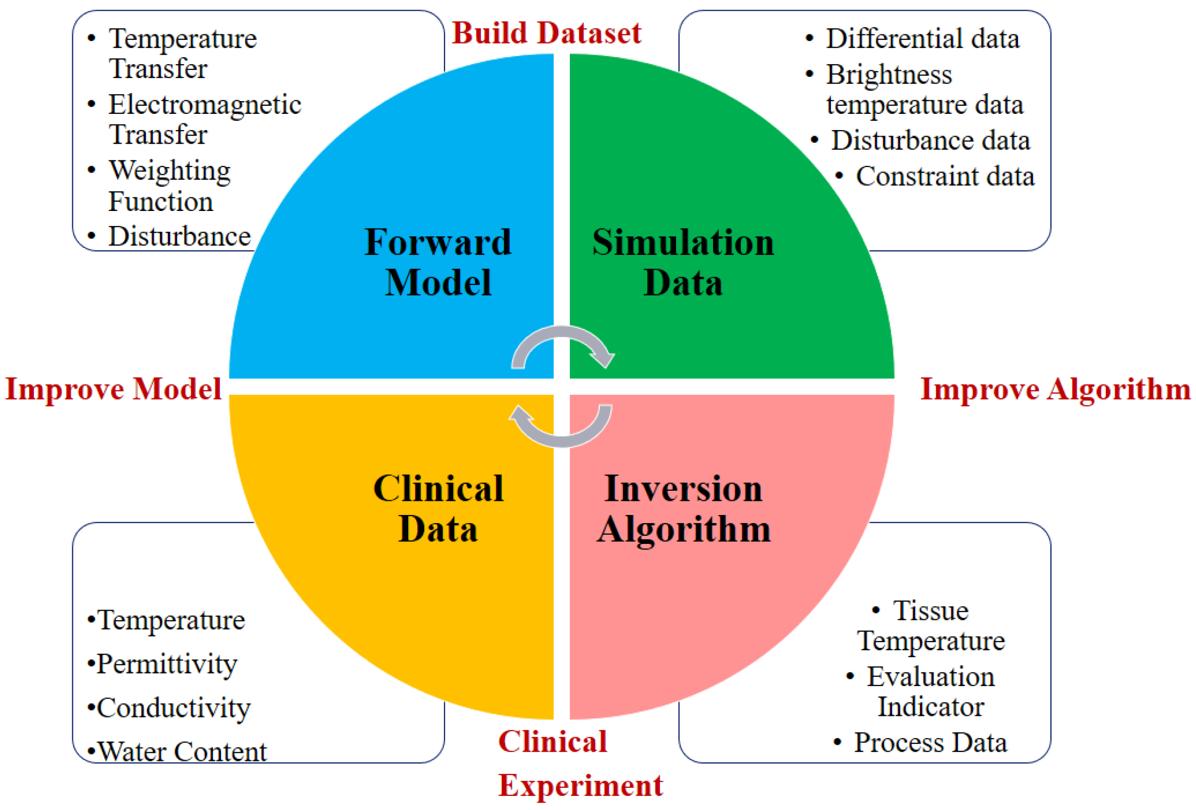
c) In order to optimize the accuracy, generalization and robustness of the inversion algorithm, a closed-loop high-precision forward and inversion modeling detection method for human tissue temperature measurement is proposed, as shown in Figure 5. Firstly, the human tissue temperature data set and constraint conditions are constructed by the forward model, then the human simulated tissue fluid, skin tissue and other samples are tested, and the clinical data are collected to verify the inversion algorithm. Finally, the clinical experiment is guided by the test results and evaluation indicators, and the mathematical and physical relationship of the forward model is improved by comparing the clinical data with the simulation data, which further enhances the scientific nature of the method.
4. Conclusion
Based on the analysis of current research, although many researchers have extensively studied the architecture of microwave radiation meters and inversion algorithms, there are still several limitations and gaps. These include inaccuracies in temperature measurement, near-field radiation characteristics of the antenna, uncertainty in brightness temperature calibration, the contribution of skin tissue temperature to weight, and a lack of research on forward and inversion modeling to detect the stratified temperature of skin tissue. This research proposes a precise temperature measurement scheme for human skin tissue using a multi-band closed-loop forward and inversion modeling approach. However, there are still some key technologies that need to be urgently addressed in the scheme. For instance, optimizing the pencil beam radiation characteristics of the temperature measuring antenna by combining the quantitative model of calibration link uncertainty, and characterizing the relationship between the key unit parameters of the system and the temperature measurement performance. Focusing on constructing the accurate temperature measurement mechanism of human skin tissue in forward and inversion modeling and solving the influence of many variable parameters and nonlinear scattering of the measured object on the temperature measurement accuracy, so as to realize a set of early diagnosis system of human skin tissue lesions that meets the clinical test standards, this research aims to enhance the theoretical framework of microwave radiation diagnosis technology and establish a solid theoretical foundation for its practical implementation.
Author Contributions
Jingtao Wu: Conceptualization, Writing-original draft, Investigation, Formal analysis. Jie Liu: Methodology, Supervision, Writing-reviewing and editing, Project administration.
Funding
This work was supported in part by the National Natural Science Foundation of China under Grant 62276009.
Conflicts of Interest
The authors declare no conflicts of interest.
References
- Organization W, H. Global Health Observatory; World Health Organization: Geneva, Switzerland, 2022. [Google Scholar]
- Pacheco, A.G.C.; Krohling, R.A. An Attention-Based Mechanism to Combine Images and Metadata in Deep Learning Models Applied to Skin Cancer Classification. IEEE J BIOMED HEALTH, 2021, 25, 3554–3563. [Google Scholar] [CrossRef]
- Al-Nuaimi, M.K.T.; Hong, W.; Zhang, Y. Design of High-Directivity Compact-Size Conical Horn Lens Antenna. In IEEE An-tennas and Wireless Propagation Letters; IEEE: Greenvile, SC, USA, 2014; Volume 13, pp. 467–470. [Google Scholar] [CrossRef]
- Rodrigues, D.B.; Maccarini, P.F.; Salahi, S.; Oliveira, T.R.; Pereira, P.J.S.; Limao-Vieira, P.; Snow, B.W.; Reudink, D.; Stauffer, P.R. Design and Optimization of an Ultra Wideband and Compact Microwave Antenna for Radiometric Monitoring of Brain Temperature. IEEE Trans. Biomed. Eng. 2014, 61, 2154–2160. [Google Scholar] [CrossRef] [PubMed]
- Sun, G.M.; Ma, P.; Liu, J. , et al. Design and Implementation of a Novel Interferometric Microwave Radiometer for Human Body Temperature Measurement. SENSORS-BASEL, 2021, 21, 1619. [Google Scholar] [PubMed]
- Ma, J.Y.; Liu, J.; Tian, Y.P. , et al. Design and Implementation of Ku-Band High Directionality Antenna. IEEE T ANTENN PROPAG, 2022, 70, 11514–11525. [Google Scholar]
- Budhu, J.; Rahmat-Samii, Y. A Novel and Systematic Approach to Inhomogeneous Dielectric Lens Design Based on Curved Ray Geometrical Optics and Particle Swarm Optimization. IEEE Trans. Antennas Propag. 2019, 67, 3657–3669. [Google Scholar] [CrossRef]
- Wu, Q.; Wang, H.; Hong, W. Multi-Stage Collaborative Machine Learning and Its Application to Antenna Modeling and Optimization. IEEE T ANTENN PROPAG, 2020, 67, 1659–1668. [Google Scholar]
- Yuan, L.; Yang, X.S.; Wang, C. , et al. Multibranch Artificial Neural Network Modeling for Inverse Estimation of Antenna Array Directivity. IEEE T ANTENN PROPAG, 2020, 68, 4417–4427. [Google Scholar]
- Yuan, L.; Wang, L.; Yang, X.S. , et al. An Efficient Artificial Neural Network Model for Inverse Design of Metasurfaces. IEEE ANTENN WIREL PR, 2021, 20, 1013–1017. [Google Scholar]
- Xiao, L.Y.; Shao, W.; Jin, F.L. , et al. Multi-Parameter Modeling with ANN for Antenna Design. IEEE T ANTENN PROPAG, 2018, 66, 3718–3723. [Google Scholar]
- Xiao, L.Y.; Shao, W.; Jin, F.L. , et al. Inverse Artificial Neural Network for Multi-Objective Antenna Design. IEEE T ANTENN PROPAG, 2021, 69, 6651–6659. [Google Scholar]
- Naseri, P.; Hum, S.V. A Generative Machine Learning-Based Approach for Inverse Design of Multilayer Metasurfaces. IEEE T ANTENN PROPAG, 2021, 69, 5725–5739. [Google Scholar] [CrossRef]
- Momenroodaki, P.; Haines, W.; Fromandi, M.; Popovic, Z. Noninvasive Internal Body Temperature Tracking With Near-Field Microwave Radiometry. IEEE Trans. Microw. Theory Tech. 2017, 66, 2535–2545. [Google Scholar] [CrossRef]
- Goryanin, I.; Karbainov, S.; Shevelev, O.; Tarakanov, A.; Redpath, K.; Vesnin, S.; Ivanov, Y. Passive microwave radiometry in biomedical studies. Drug Discov. Today 2020, 25, 757–763. [Google Scholar] [CrossRef] [PubMed]
- Chen, R.H.; Luo, J.; Hu, A.Y. , et al. Uniform Circular Multiphase Modulation Correlation Radiometer and Its Sensitivity Analysis. Journal of Beijing University of Aeronautics and Astronautics, 2023, 49, 1857–1863. [Google Scholar]
- Sun, G.M.; Liu, J.; Ma, J.Y. , et al. Design and Implementation of Multiband Noncontact Temperature-Measuring Microwave Radiometer. MICROMACHINES-BASEL, 2021, 12, 1202. [Google Scholar] [PubMed]
- Liu, J.; Zhang, R.Q.; Sun, G.M. , et al. Design and Implementation of High Sensitivity Microwave Radiometer. AEU-INT J ELECTRON C, 2023, 170, 1–10. [Google Scholar]
- Chen, R.H.; Luo, J.; Hu, A.Y. , et al. Uniform circular multiphase modulation correlation radiometer and its sensitivity analysis. Journal of Beijing University of Aeronautics and Astronautics, 3, 49, 1857-1863 (in Chinese).
- Jacob, K.; Schroder, A.; Murk, A. Design, Manufacturing, and Characterization of Conical Blackbody Targets With Optimized Profile. IEEE Trans. Terahertz Sci. Technol. 2017, 8, 76–84. [Google Scholar] [CrossRef]
- Houtz, D.A.; Emery, W.; Gu, D.; Walker, D.K. Brightness Temperature Calculation and Uncertainty Propagation for Conical Microwave Blackbody Targets. IEEE Trans. Geosci. Remote. Sens. 2018, 56, 7246–7256. [Google Scholar] [CrossRef]
- Schroder, A.; Murk, A.; Wylde, R.; Schobert, D.; Winser, M. Brightness Temperature Computation of Microwave Calibration Targets. IEEE Trans. Geosci. Remote. Sens. 2017, 55, 7104–7112. [Google Scholar] [CrossRef]
- Virone, G.; Addamo, G.; Bosisio, A.V.; Zannoni, M.; Valenziano, L.; Rizzo, D.; Radaelli, P. Thermal Vacuum Cold Target for the Metop SG MicroWave Imager. IEEE J. Sel. Top. Appl. Earth Obs. Remote. Sens. 2021, 14, 10348–10356. [Google Scholar] [CrossRef]
- Jin, M.; Yuan, R.; Li, X. , et al. Wideband Microwave Calibration Target Design for Improved Directional Brightness Temperature Radiation. IEEE GEOSCI REMOTE S, 2022, 19, 1–5. [Google Scholar]
- Liu, J.; Sun, Z.L.; Sun, G.M. , et al. Design and Implementation of a Ku-Band High- Precision Blackbody Calibration Target. MICROMACHINES-BASEL. 2023, 14, 18. [Google Scholar]
- Scheeler, R. A Microwave Radiometer for Internal Body Temperature Measurement. University of Colorado at Boulder, 2013.
- Popovic, Z.; Momenroodaki, P.; Scheeler, R. Toward wearable wireless thermometers for internal body temperature measurements. IEEE Commun. Mag. 2014, 52, 118–125. [Google Scholar] [CrossRef]
- He, F. Study of Nondestructive Retrieval Method for the Measurement of Human Internal Temperature by Microwave. Huazhong University of Science and Technology, 2015.
- Qian, P.C.; Barry, M.A.; Lu, J.T. , et al. Transcatheter Microwave Ablation Can Deliver Deep and Circumferential Perivascular Nerve Injury Without Significant Arterial Injury to Provide Effective Renal Denervation. J HYPERTENS, 2019, 37, 2083–2092. [Google Scholar] [PubMed]
- Scheeler, R.; Kuester, E.F.; Popovic, Z. Sensing Depth of Microwave Radiation for Internal Body Temperature Measurement. IEEE Trans. Antennas Propag. 2013, 62, 1293–1303. [Google Scholar] [CrossRef]
- Liu, J.; Zhang, K.; Ma, J.Y. , et al. High-Precision Temperature Inversion Algorithm for Correlative Microwave Radiometer. SENSORS-BASEL, 2021, 21, 5336. [Google Scholar] [PubMed]
- Lin, X.; Ding, Y.; Gong, Z. , et al. Hybrid Microwave Medical Imaging Approach Combining Quantitative and Qualitative Algorithms. IEEE Antennas and Wireless Propagation Letters, 2021, 20, 438–442. [Google Scholar]
- Tisdale, K.; Bringer, A.; Kiourti, A. A Core Body Temperature Retrieval Method for Microwave Radiometry When Tissue Permittivity is Unknown. IEEE J. Electromagn. Rf Microwaves Med. Biol. 2022, 6, 470–476. [Google Scholar] [CrossRef]
- Tisdale, K.; Bringer, A.; Kiourti, A. Development of a Coherent Model for Radiometric Core Body Temperature Sensing. IEEE J. Electromagn. Rf Microwaves Med. Biol. 2022, 6, 355–363. [Google Scholar] [CrossRef]
- Groumpas, E.; Koutsoupidou, M.; Karanasiou, I.S.; Papageorgiou, C.; Uzunoglu, N. Real-Time Passive Brain Monitoring System Using Near-Field Microwave Radiometry. IEEE Trans. Biomed. Eng. 2019, 67, 158–165. [Google Scholar] [CrossRef]
- Issac, J.P.; Sugumar, S.P.; Arunachalam, K. Self-Balanced Near-Field Microwave Radiometer for Passive Tissue Thermometry. IEEE Sensors J. 2022, 22, 6544–6552. [Google Scholar] [CrossRef]
- Streeter, R.; Botello, G.S.; Hall, K. , et al. Correlation Radiometry for Subcutaneous Temperature Measurements. IEEE J ELECTROMAG RF, 2022, 6, 230–237. [Google Scholar]
- Chen, C.; Zhang, J.Q.; Lu, T.Y. , et al. Secret Key Generation for IRS-Assisted Multi-Antenna Systems: A Machine Learning-Based Approach. IEEE T INF FOREN SEC, 2024, 19, 1086–1098. [Google Scholar]
- Zhu, D.; Tao, J.Y. , Su J. L., et al. BlockMFRAs: Block-Wise Multiple-Fold Redundancy Arrays for Joint Optimization of Radiometric Sensitivity and Angular Resolution in Interferometric Radiometers. IEEE T GEOSCI REMOTE, 2024, 62, 1–15. [Google Scholar]
- Einizade, A.; Sardouie, S.H. Iterative Pseudo-Sparse Partial Least Square and Its Higher Order Variant: Application to Inference From High-Dimensional Biosignals. IEEE Trans. Cogn. Dev. Syst. 2023, 16, 296–307. [Google Scholar] [CrossRef]
Figure 1.
The principle and system composition block diagram of microwave radiation diagnosis technology.
Figure 1.
The principle and system composition block diagram of microwave radiation diagnosis technology.
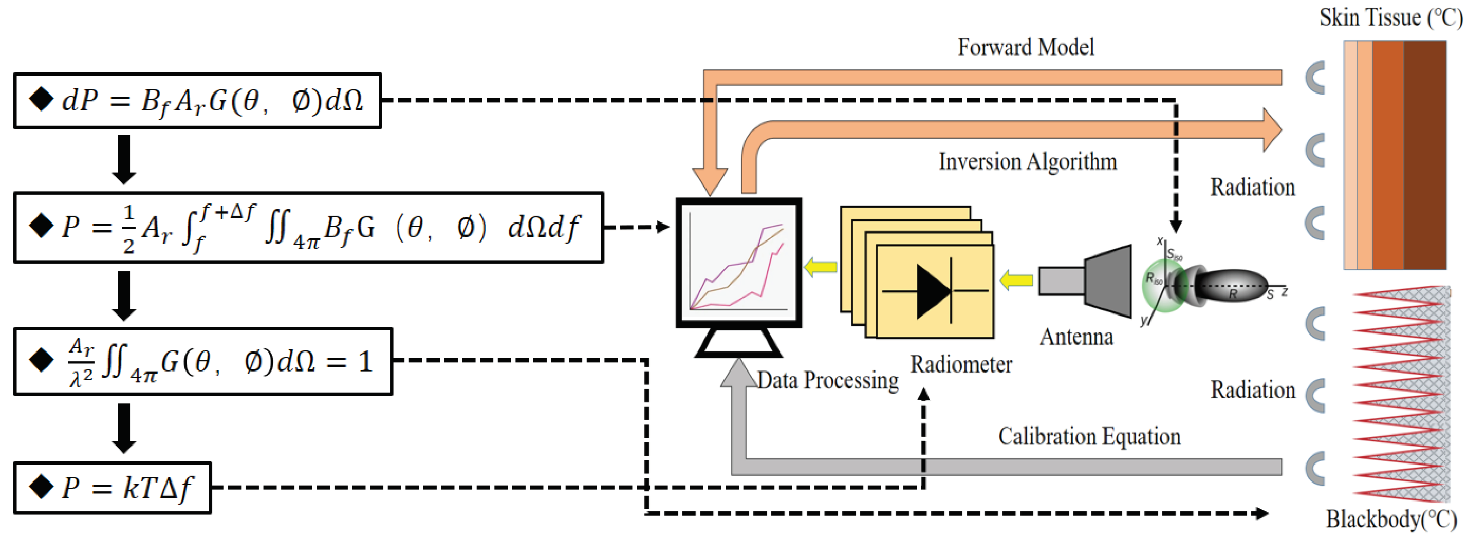
Figure 2.
Neural network model based on prior knowledge in this research.
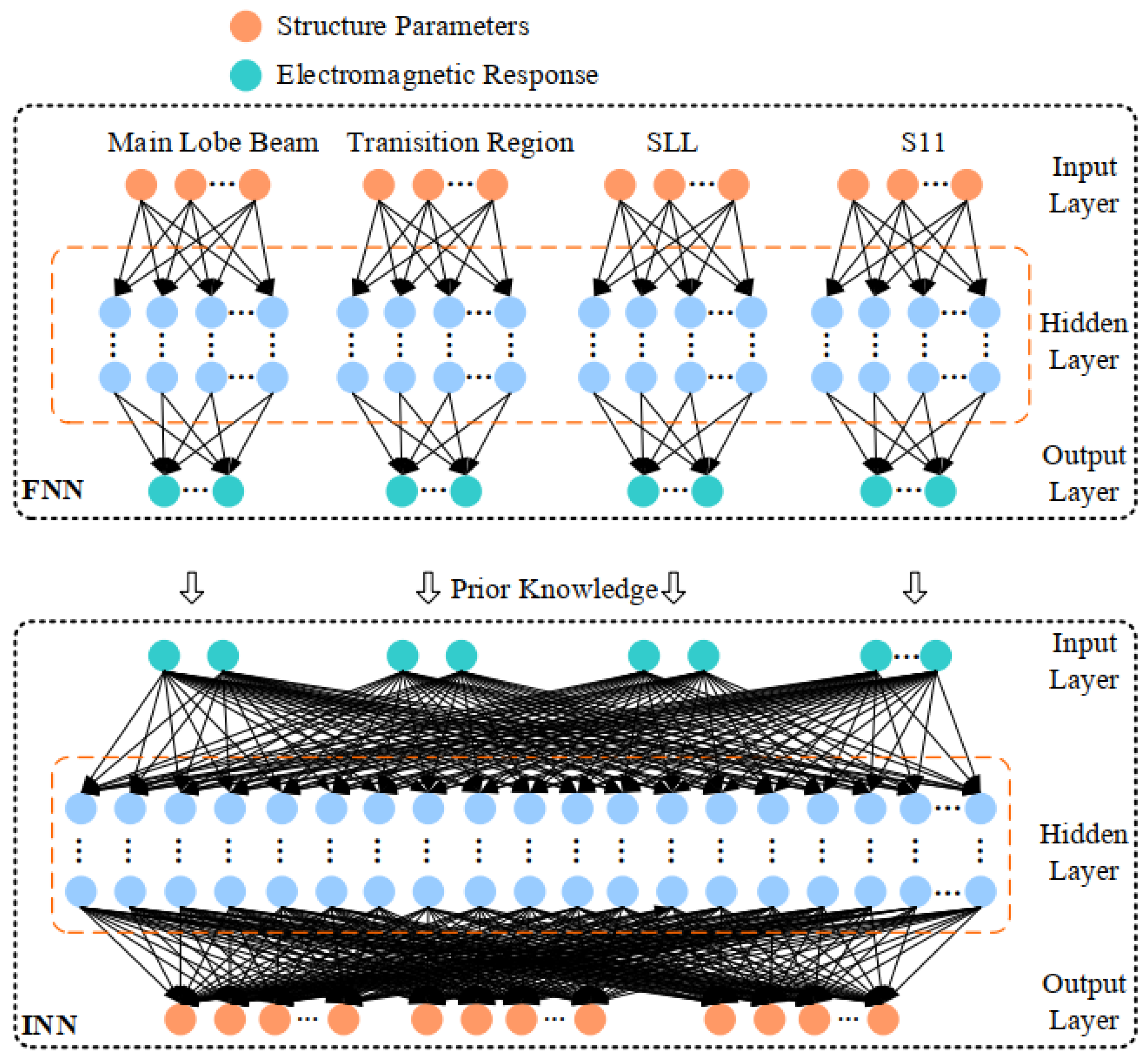
Figure 3.
Schematic diagram of the calculation of the brightness temperature of the coating array calibration source directional radiation scene.
Figure 3.
Schematic diagram of the calculation of the brightness temperature of the coating array calibration source directional radiation scene.
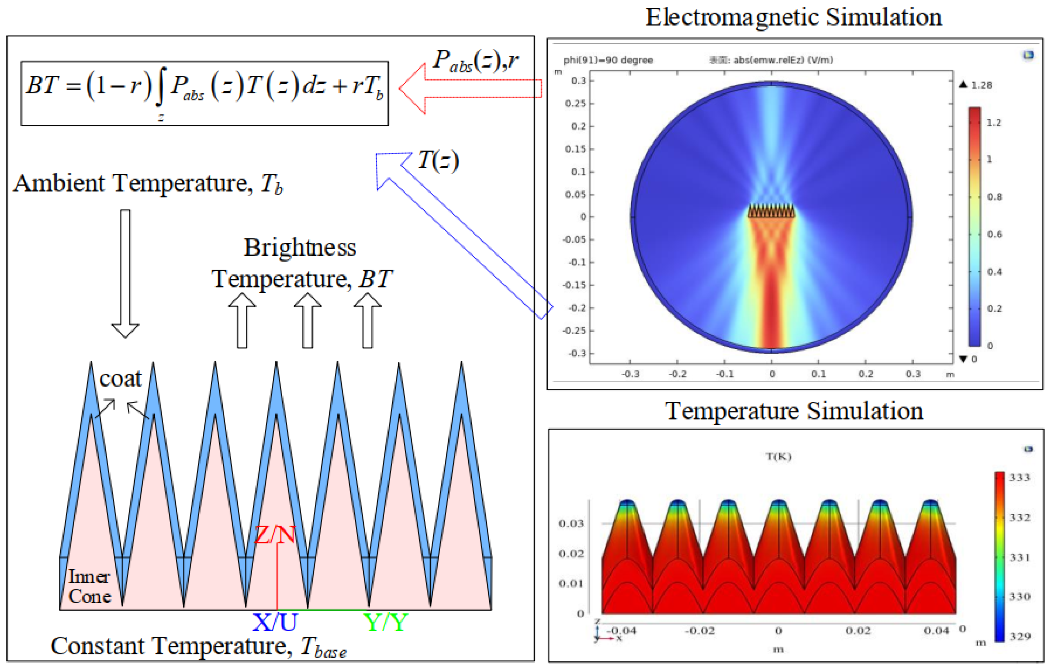
Figure 4.
(a) Incoherent model of microwave thermal radiation between human skin tissues; (b) microwave thermal radiation model of human body surface wearing clothes.
Figure 4.
(a) Incoherent model of microwave thermal radiation between human skin tissues; (b) microwave thermal radiation model of human body surface wearing clothes.
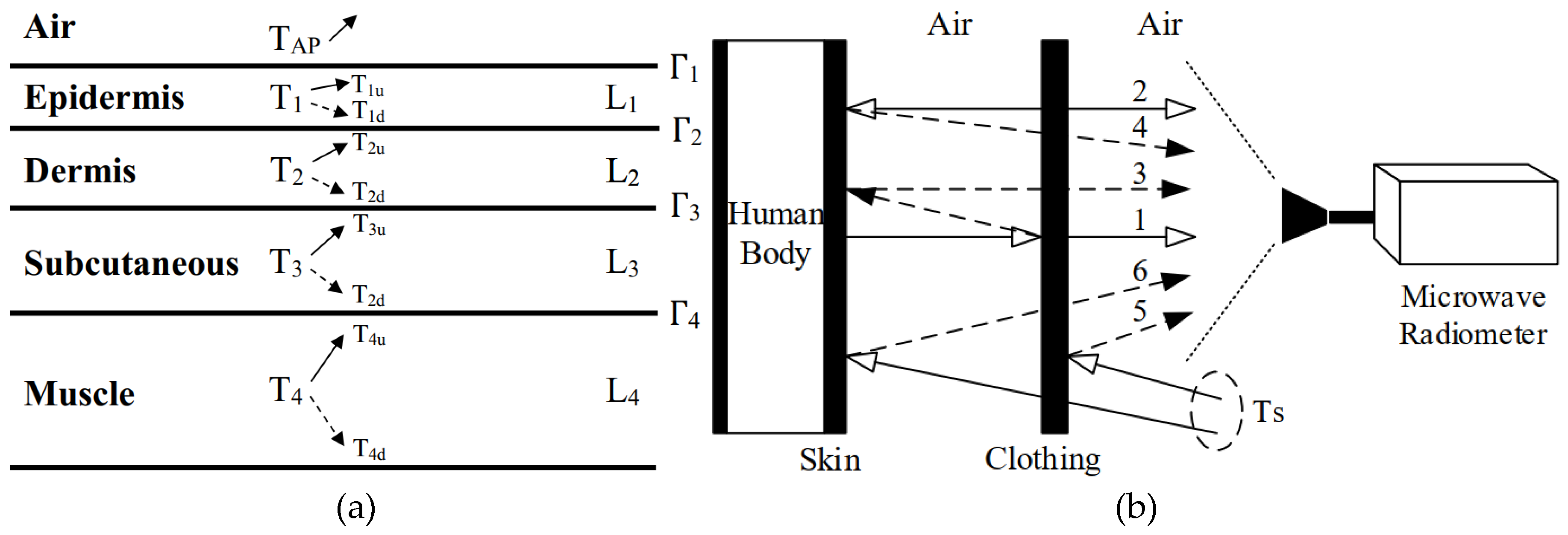
Figure 5.
Closed-loop high-precision forward and inversion modeling detection method for human tissue temperature measurement.
Figure 5.
Closed-loop high-precision forward and inversion modeling detection method for human tissue temperature measurement.
Disclaimer/Publisher’s Note: The statements, opinions and data contained in all publications are solely those of the individual author(s) and contributor(s) and not of MDPI and/or the editor(s). MDPI and/or the editor(s) disclaim responsibility for any injury to people or property resulting from any ideas, methods, instructions or products referred to in the content. |
© 2024 by the authors. Licensee MDPI, Basel, Switzerland. This article is an open access article distributed under the terms and conditions of the Creative Commons Attribution (CC BY) license (https://creativecommons.org/licenses/by/4.0/).
Copyright: This open access article is published under a Creative Commons CC BY 4.0 license, which permit the free download, distribution, and reuse, provided that the author and preprint are cited in any reuse.


