Submitted:
01 March 2024
Posted:
04 March 2024
You are already at the latest version
Abstract
Diabetic retinopathy (DR) is the primary factor leading to vision impairment and blindness in diabetic people. Uncontrolled diabetes can damage the retinal blood vessels. Initial detection and prompt medical intervention are vital in preventing progressive vision impairment. Today's growing medical field poses more significant workload and diagnostic demands on medical professionals. In the proposed study, a convolutional neural network (CNN) is employed to detect the stages of DR. This research is crucial for studying DR because of its innovative methodology incorporating two different public datasets. This strategy enhances the model's capacity to generalize unseen DR images, as each dataset encompasses unique demographics and clinical circumstances. The network can learn and capture complicated hierarchical image features with asymmetric weights. Each image undergoes preprocessing using contrast-limited adaptive histogram equalization (CLAHE) and the discrete wavelet transform (DWT). The model is trained and validated using the combined datasets of Dataset for Diabetic Retinopathy (DDR) and the Asia Pacific Tele-Ophthalmology Society (APTOS). The CNN model is tuned with different learning rates and optimizers. The CNN model with Adam optimizer achieved 70% accuracy and an area under curve (AUC) score of 0.82. The recommended study results may reduce diabetes-related vision impairment by early DR severity identification.
Keywords:
artificial intelligence
; convolutional neural networks
; diabetic retinopathy
; deep learning
; medical image analysis
1. Introduction
Diabetes is a debilitating and persistent condition characterized by insufficient production or use of insulin in the body. The count of individuals with diabetes overall is supposed to increase from 536.6 million in 2021 to 783.2 million individuals aged 20 to 79 by 2045 [1]. Type 1 and Type 2 are the two forms of diabetes. Retinopathy usually strikes 60% of type 2 diabetes patients and nearly all type 1 diabetes patients in the 20 years after diagnosis. The worldwide occurrence of diabetes has been reported to be 9.8% [2].
Diabetic retinopathy (DR) is the main underlying factor behind worldwide vision loss. It impacts around 33% of individuals who have been diagnosed with diabetes. Consequently, timely diagnosis and therapy of DR can significantly diminish the likelihood of permanent visual impairment, floaters in the eye, and eventual loss of eyesight. Within 20 years after being diagnosed, retinopathy impacts around 60% of patients with type 2 diabetes and nearly all those with type 1 diabetes. Nevertheless, DR can progress without exhibiting any symptoms until it poses a risk to vision.
Manually inspecting and determining the severity of DR requires a significant amount of time that is prone to errors. Precise evaluation of DR’s impact requires highly experienced ophthalmologists’ skills [3]. The screening approach depends on an expert’s evaluation of color fundus photographs, misdiagnosing several instances and causing a delay in treatment [4].
Medical imaging has employed deep-learning algorithms for disease screening and detection. Diverse approaches are used to identify DR at its earlier stages, with machine learning playing a significant part in this effort. Artificial intelligence employs machine learning techniques to enhance the learning process independently, eliminating the requirement for direct human interaction. Deep learning is often used in predicting medical conditions [5]. Many fields, including computer vision, medical image analysis, and fraud detection systems, offer advantages for deep learning and machine learning [6,7].
Deep learning extracts fundamental features from massive datasets utilizing feature extraction, which data mining tools assess and predict. These algorithms anticipate optimal, exact outputs, simplifying early illness forecasts and saving millions of lives [8]. Computer vision and medical image processing applications, notably CNNs [8,9,10,11,12], have extensively used deep learning techniques.
Most conventional techniques cannot reveal hidden characteristics and their relationships. Instead of learning valuable information, it retains useless features like size, brightness, and rotation, which decreases performance and accuracy [13]. Another concern is that understanding the little unnecessary information in retinal images causes the model’s ability to generalize and adapt to other datasets [14].
Non-Proliferative (NonPrDR) and Proliferative (PrDR) are the two primary stages of DR. The NonPrDR refers to the initial stages of DR and can be mild, moderate, and severe. Conversely, PrDR is the advanced stage of the illness. Many people do not get symptoms until the disease progresses to the PrDR stage [15]. Figure 1 shows several stages of retinal imaging with DR from the APTOS dataset [16].
The combination of machine learning and deep learning indicates the potential to transform the categorization of DR [17]. However, there is an increasing demand for automated technologies that can efficiently evaluate vast datasets while maintaining high levels of accuracy due to the growing volume of collected patient data. The demand for efficient and cost-effective techniques for early identification of diabetic retinopathy is of utmost importance [18]. As each dataset varies in demographics and clinical situations, this research is essential to the study of DR because it employs a unique strategy that combines two different datasets to improve the model’s capacity to generalize the unseen DR images.
Our work aimed to develop a deep learning model that successfully predicts DR images using a CNN model. The model was trained, validated, and tested on APTOS-DDR fundus datasets. The images were preprocessed using CLAHE to perform histogram equalization and then to DWT to extract the coefficients. The CNN model can extract the relevant information or features from the preprocessed images. To train the model, a multi-class classification technique categorizes DR into five stages: normal or no DR, mild, moderate, severe, and PrDR. Limited academic research evaluates CLAHE and DWT with combined datasets, focusing on their performance in categorizing DR stages.
Significant contributions to this study include:
- The study utilized two public datasets, including APTOS and DDR, to categorize each stage of DR. The APTOS and DDR datasets were merged to train, validate, and test the model. To mitigate the issue of generalizability, one can address it by blending diverse datasets and evaluating the model’s performance on an unseen test set.
- A CNN model has been constructed to predict DR stages. The learning rate is tuned during the model training, and optimizers such as Adaptive moment estimation (Adam), Root mean square propagation (RMSProp), Adamax, Adaptive gradient algorithm (Adagrad), and stochastic gradient descent (SGD) are evaluated on the model. Data augmentation is used in the training set to mitigate the issue of overfitting.
- We provide a novel image classification framework that carefully blends many effective processing algorithms to improve classification performance. Each image undergoes preprocessing using CLAHE. By altering the intensity distribution in specific regions of the picture, this approach enhances the contrast of an image. We then employ the DWT to divide images into frequency components to recover spatially covered features.
- Our methodology also offers new research paths, notably in integrating DWT with other deep learning architectures and applying it to complicated image processing problems.
The consequent portions of the article are categorized as follows: The background research in section two shows the literature review of the DR, followed by Section 3, an overview of the methodology used in the investigation. The results are given and examined in part 4, and Section 5 discusses them. Finally, part six provides a conclusion to the study.
2. Literature Review
Deep learning has been employed in medical imaging for illness diagnosis. Several research papers have investigated the prediction of DR utilizing CNN and pre-trained models, including DenseNet, VGG, ResNet, and Inception [19]. Moreover, specific study is required to enhance the efficiency of the deep learning framework [20]. With 94.4% accuracy, Usman et al. [4] observed that a pre-trained CNN model detected lesions better. The researchers used principal component analysis to characterize fundus pictures.
Gargeya and Leng [21] introduced a sophisticated automated technique for identifying DR using deep learning methods. It offers a neutral alternative for detecting DR that can be used on any device. Another work by Areeb and Nadeem [22] categorizes DR photos using support vector machines and random forest methods, with convolutional layers employed to extract features. The analysis revealed that random forest had high sensitivity and specificity, surpassing other approaches in performance.
The surge in transfer learning over the past few years can be linked to the scarcity of supervised learning options for a diverse array of practical scenarios and the abundance of pre-trained models. Several research has constructed DR models utilizing VGG16 [23,24], DenseNet [25], InceptionV3 [26], and ResNet [27]. In their study, Qian et al. [28] utilized transfer learning and attention approaches to classify DR and obtained an accuracy rate of 83.2%. Another paper [25] utilized a “convolutional block attention module (CBAM)” in conjunction with the APTOS dataset. The DR grading exercise was completed with an accuracy rate of 82%.
Zhang et al. [29] employed a limited retinal dataset to refine a pre-existing CNN model using a process known as fine-tuning. Using the EyePACS and Messidor datasets, they outperformed previous DR grading techniques regarding accuracy and sensitivity. The research authors [30] investigated DR classification by combining Swin with wavelet transformation. Their performance reached an accuracy rate of 82%, along with a sensitivity of 0.4626. An attention model was used in conjunction with a pretrained DenseNet model by Dinpajhouh and Seyyedsalehi to determine the severity of DR utilizing the APTOS database [31]. The evaluation resulted in an accuracy of 83.69%.
A machine-learning approach was suggested to determine the main causes of DR in individuals with elevated glucose levels [32]. Employing transfer learning approaches, this process isolates and organizes the features of DR into many classes. Before the classification phase, the entropy technique selects the most distinguishing attributes from a set of features. The model’s objective is to ascertain the level of severity in the patient’s eye, and it will be valuable in precisely categorizing the severity of DR. The study conducted by Murugappan et al. [33] utilized a Few-Shot Learning approach to develop a tool for detecting and evaluating DR. The approach employs an attention mechanism and episodic learning to train the model with limited training data. When evaluated on the APTOS dataset, the model achieves high DR classification and grading regarding accuracy and sensitivity.
CNN’s U-Net architecture is utilized for image segmentation applications [34]. The study by Jena et al. [35] employed an asymmetric deep learning architecture utilizing U-Net architecture for DR image segmentation. The pictures from the green channel are utilized to analyze and thus improve the performance using CLAHE. The paper [36] presents a computerized system that utilizes a mix of U-Net and transfer learning to diagnose DR automatically from fundus pictures. The researchers utilize the Kaggle DR Detection dataset, which is accessible to the public, and improve an Inception V3 model that has already been trained to extract features. The collected characteristics are subsequently input into a U-Net model to partition the retina and optic disc. Divided into segments, the pictures are further categorized into five degrees of DR severity using a multi-layer perceptron classifier. On the Kaggle dataset, their strategy outperforms other cutting-edge techniques with an accuracy of 88.3%.
Transfer learning has been utilized in the domain of DR to overcome the limitation of having little annotated data available to train models based on deep learning. The researchers utilized AlexNet, InceptionV3, VGG16, DenseNet169, VGG19, and ResNet50, trained on large datasets like ImageNet, as feature extractors for DR pictures [36,37,38,39,40]. To achieve high precision in DR classification, the pre-existing models were adjusted and optimized using a labeled dataset specifically designed for DR, such as the APTOS, EyePACS, and Messidor datasets. C. Zhang et al. [29] conducted another investigation that suggested a transfer learning method for assessing diabetic retinopathy without needing a source. The researchers employed a pre-trained CNN model and adjusted its parameters on a limited number of retinal pictures without needing more source data. The evaluation uses the EyePACS and Messidor datasets, surpassing other cutting-edge methodologies regarding accuracy and sensitivity in assessing DR.
Data augmentation is widely regarded as the predominant technique for addressing the problem of imbalanced data in image classification tasks [41]. It involves creating new data components from current data to enhance the data artificially. Image augmentation techniques, such as cropping, rotating, zooming, vertical and horizontal flip, width shift, and rescaling, can modify the pictures [42]. Mungloo-Dilmohamud [43] found that the quality of transfer learning in DR classification is enhanced using a data augmentation technique. Different datasets and CLAHE techniques were employed by Ashwini et al. [44] for detecting DR. The images were preprocessed using the DWT method. According to their study, the individual datasets performed better than combined datasets.
In a study by Dihin et al. [45], a wavelet transform with a shifted window model is utilized on the APTOS dataset. Compared to binary classification, which has 98% accuracy, the multi-class classification has reached only 86% accuracy. Image segmentation was carried out by Cornforth et al. [46], who employed a combination of wavelet assessment, supervised classifier likelihoods, adaptive threshold methods, and morphology-based approaches. Different retinal diseases were monitored by Yagmur et al. [47] by incorporating the DWT in image processing. Another study by Rehman et al. [48] applied DWT with different machine learning classifiers, such as k-nearest neighbors (KNN) and support vector machine (SVM) models. They used Messidor data with binary classification.
The challenges of DR detection include proper image processing methods and developing accurate models that can detect different datasets [49]. Most of the studies employed a single image set for training and testing. The common performance measures used to analyze are accuracy, recall or sensitivity, and precision [50]. Table 1 describes the inference related to previous DR-related studies.
3. Materials and Methods
The workflow of the study is shown in Figure 2. The stages involved collecting retinal images from public data, preprocessing the images, designing the model, training and validating the model with fine-tuning, and testing the model with an external dataset.
3.1. Dataset
The dataset employed in this study is public access data. The APTOS [16] and DDR [60] data are combined for training, testing, and validation. The APTOS dataset contains 3662 photos, each accompanied by its corresponding label. The DDR dataset has 12,524 images depicting various stages of DR. The two datasets are merged, resulting in 16,186 images fed into the model with five labels (no DR, mild, moderate, severe, and PrDR). However, 16 images were excluded from the dataset due to missing valid image names in the file, so a total of 16,170 images are employed in the study.
The class label no Dr (class 0) has 8062 images, mild DR (class 1) has 999 images, moderate DR (class 2) has 5472 images, severe DR (class 3) has 429 images, and PDR (class 4) has 1208 images. Following a 70:15:15 data split, 11,682 images are utilized for training, 2062 images are employed for validation, and 2426 images for testing. The complete count for each class is depicted in Table 2.
3.2. Data Augmentation
Deep learning methods exhibit optimal performance when applied to large-scale data sets. Typically, the model’s performance is improved with more data. Whether it is images or data, data augmentation is used to complement the model’s training data. Each image will be assigned an identical label as the original image from which it was generated. Before subjecting the dataset to the model, more images were incorporated into the training set to rectify the imbalance [41].
Different techniques involve rotating an image, image shifting, flipping, zooming, and applying brightness. This proposed study applies properties such as image rotation with 40 degrees, width shift with a value of 0.2, height shift with 0.2, and horizontal flipping on the training set. Figure 3 shows the augmented images of a random sample image.
3.3. Image Preprocessing
Image preprocessing is crucial for machine learning and deep learning to function effectively in their respective domains. During the preprocessing stage, it is customary to normalize images by rescaling them to the range [0, 1], ensuring that they have an average of zero and a standard deviation of 1. Scaling input data involves standardizing it, which promotes faster learning and convergence in neural networks.
CLAHE is an image processing method employed to enhance the contrast and visibility of fine features in images, particularly those that exhibit uneven lighting conditions or poor contrast. CLAHE prevents contrast over-amplification in adaptive histogram equalization (AHE). Tiles, not the complete image, are what CLAHE processes. It removes spurious borders by combining nearby tiles using bilinear interpolation. This method boosts visual contrast [57]. CLAHE may also be used to color photos, mainly to the luminance channel, which yields better results than total channel equalization in BGR images. Initially, CLAHE enhanced the quality of medical images with low contrast.
Contrary to typical AHE, CLAHE restricts contrast. The CLAHE established a clipping limit to alleviate the problem of noise amplification [61]. In this study, after applying CLAHE preprocessing, the images were resized to a similar size. The image size varies in each dataset; for example, APTOS images are 3216x2136 pixels, and DDR has 512x512 pixels. So, to make it similar, the image size parameter is set to 150x150 pixels. Then, the DWT method is applied to each image and rescaled to [0,1].
3.3.1. Discrete Wavelet Transform
A mathematical method for processing signals and images, the Discrete Wavelet Transform (DWT) allows the examination of distinct signal components at varying resolutions or scales. In particular, the DWT breaks down a signal into two sets of coefficients: approximation coefficients and detail coefficients, which stand for the signal’s low-frequency and high-frequency components, respectively [62]. In frequency, among the most often used techniques for image processing is the wavelet transform, which allows the information contained in images to be represented collectively [63]. Using the Python wavelet framework, the DWT is represented by
where cA represents approximation coefficients, cH is the horizontal coefficients, cV is the vertical coefficients, and cD is the diagonal coefficients. Here cH, cV, and cD are the detailed coefficients.
The first step in the DWT method is to run the original image through two filters: a high-pass filter to extract the cV, cH, and cD and a low-pass filter to extract the cA component, as shown in Equation (1). These filters aid in separating the signal’s fine and coarse features. Following filtering, a downsampling of two is applied to both sets of coefficients, reducing the image resolution to half.
3.4. The Deep Learning Model
The proposed model aims to precisely classify and predict DR stages by analyzing the image. The input image preprocessed data is used as features, while the label supplied to each image acts as the target variable. Multiple filters and layers extract image information and attributes throughout the feature extraction process. Following this stage, the images are categorized based on the desired target labels. The recommended model’s architecture is seen in Figure 4.
The input layer is modified by reshaping it to include three channels, which correspond to the red, green, and blue channels of the RGB color model. The picture dimensions are adjusted using 150 (width and height) values. The preprocessed image (with CLAHE and DWT applied) is fed into the CNN model. The image resolution reduces to half after applying DWT method.
Convolutional layers have convolution operations to summarize and minimize information features. The feature map output shows picture corners and edges. Later, further layers use this feature map to learn more input image features. The pooling layer reduces convolved feature map size to reduce computational expenses. It is done by lowering layer connections and separately operating on each feature map. The kernel size is 3, and the units of each convolutional layer are 16, 32, 64, and 128, respectively. The activation function employed is ‘relu’. Max Pooling uses the most significant feature map element with a pool size of two. BatchNormalization in neural networks is a technique that normalizes the activation levels between layers. It helps to improve the efficiency and accuracy of model training by using regularization. The Flatten layer reduces the dimensionality of the previous layer’s pictures by flattening the last layer’s results.
The fully connected layers consist of two dense layers. The first dense layer has 256 units, and the activation function is ‘relu’. The model’s overfitting is mitigated by including a dropout layer set at a frequency rate of 0.5. These layers are then connected to the output dense layer, which has ‘softmax’ activation and is designed to classify data into five different DR stages. The loss function is sparse categorical entropy, as the class labels are considered integers.
3.4.1. Model Optimizer
Optimization methods are essential to machine and deep learning model training for enhancing the model’s predictions. Various techniques have been created to tackle specific optimization problems, including handling sparse gradients or quickening convergence [64]. One of the most straightforward yet most powerful optimization methods is SGD. It uses a small portion of training data to update the model’s weights instead of the entire dataset, which speeds up computation significantly. By scaling each parameter inversely proportionate to the square root of the total of all of its previous squared values, Adagrad modifies the learning rates of all parameters. Adagrad works exceptionally well with sparse data.
RMSprop uses a moving average of squared gradients to solve the Adagrad problem of declining learning rates. This technique dynamically modifies the learning rate for each parameter, increasing it for steps with small gradients to expedite convergence and decreasing it for steps with significant gradients to avoid divergence. By modifying the learning rate according to a moving average of the gradients and their squares, Adam combines the benefits of Adagrad and RMSprop. Because of its ability to traverse the optimization landscape efficiently, Adam is one of the most often used optimizers for deep learning model training. A variant of Adam based on the infinite norm is called Adamax. Despite being less popular than Adam, Adamax can be helpful in some situations when its normalizing technique has benefits.
The choice of optimizer can be influenced by the particulars of the training job and the kind of data since each optimizer has advantages and uses [65]. For example, Adagrad or RMSprop may be favored for jobs with sparse data, although Adam is frequently used due to its broad usefulness across various situations. To ascertain which optimizer is most effective in this study, we utilize all five optimizers mentioned above to evaluate the model.
3.5. Performance Measures
Accuracy in DR detection measures how often the model successfully detects positive and negative situations (Equation (2)). Precision measures how successfully the model recognizes real positive cases (actual DR) among all projected positive cases (Equation (3)). Recall, or sensitivity, (Equation (4)) measures how well the model collects and detects all real occurrences of DR, minimizing false negatives. F1-score is essential because it incorporates false positives and negatives (Equation (5)). It is beneficial when positive and negative situations are imbalanced. We may calculate the AUC (area under the curve) to see how much of the graphic is below the curve. The closer the AUC is to 1, the better the model is [66].
where truePos is true positive, trueNeg is true negative, falsePos is false positive, and falseNeg is false negative.
Accuracy = (truePos+trueNeg)/(truePos+trueNeg+falsePos+falseNeg),
Precision = (truePos)/(truePos+ falsePos),
Recall = (truePos)/(truePos+falseNeg),
F1-score = (2*truePos)/(2*truePos+falsePos+falseNeg),
4. Results
4.1. Experiment Setup
The models in this work are implemented using Python packages such as TensorFlow [67], and python wavelets [68]. The NVidia Titan V GPU is employed to deploy the model. To address the problem of overfitting, deep learning models use the EarlyStopping and ReduceLROnPlateau approaches. Seventy is the value that has been allocated to the epoch parameter. For the ReduceLROnPlateau method, the value set to the patience parameter is 2. Consider a scenario where the validation loss is constant or has an upward trend. In such a scenario, the learning rate parameter is subjected to an update that is 0.1 higher than its previous value. Suppose the validation loss in the EarlyStopping mechanism demonstrates a high loss value for ten epochs. In that case, the training process for the model is ended. Table 3 displays the training parameters of the model.
4.2. Model Evaluation
The preprocessed image is depicted in Figure 5. The APTOS-DDR combined data is employed for training and validating the model. 70% of the data is used for training and 15% for validation. The CNN layers extract the features, and the fully connected layers classify the data according to the class labels provided.
The validation accuracy and loss are displayed in Table 4. The initial learning rate is 0.001. It is tuned during the training by the model using ReduceLROnPlateau. The models utilized sparse categorical loss entropy. The Adam optimizer shows around 69% accuracy with a minimal loss of 0.8432.
The accuracy of training and validation is shown in Figure 6. The EarlyStopping parameter stops the Adam model at the 45th epoch, the RMSProp model at the 25th epoch, the SGD model at the 32nd epoch, the Adagrad model at the 17th epoch, and the Adamax model at the 29th epoch. Similarly, the loss of training and validation is depicted in Figure 7.
The test data contains 2426 images from APTOS-DDR images. The model’s performance is illustrated in Table 5. The Adam optimizer model performs better than other optimizers, with 69.51% accuracy and 0.70 recall. The F1-score is also highest in the Adam model, with a value of 0.65. It is then followed by RMSProp optimizer with 66.67% accuracy and Adagrad with 65.05% accuracy.
Finally, the results are plotted in Figure 8 so that each model’s comparison with the test dataset can be visualized easily.
As AUC approaches 1, the model becomes more accurate. The AUC score of the models is depicted in Table 6. The AUC score shows that all models are good enough to classify the labels. Adam optimizer model shows a 0.8153 AUC score.
5. Discussion
The proposed study employs a CNN model with preprocessing methods such as CLAHE and DWT (Figure 4). The model predicts five stages of DR. Not all previous studies utilized different datasets for evaluation, which lacks the model’s generalizability. Significantly, few studies are related to CLAHE and DWT preprocessing with DR image data. Adam is frequently used due to its broad usefulness across various situations. Because of its ability to traverse the optimization landscape efficiently, Adam is one of the most often used optimizers for deep learning model training [64]. The performance comparison of the study with previous research is illustrated in Table 7.
5.1. Limitation and Future Works
The model is tuned only for two parameters, namely, the learning rate and optimizers. CNN with four layers was employed only in this study. Understanding the image quality and using pretrained models is one of the future enhancements of the study. Another future work direction is to collect a local dataset and evaluate the model’s performance.
6. Conclusions
Classifying DR into five stages using retina images is a complex area of research. Despite extensive efforts to classify DR as binary or multi-classes, these methods have been ineffective in reliably detecting its early stages from retinal pictures. Traditional approaches take longer and have limited prediction accuracy, making it impossible to identify early on. CNN is a popular image analysis network. The adoption of CLAHE and DWT aims to enhance the clarity of the images, facilitating the CNN model’s extraction of the most distinctive aspects. Potentially contributing to preventing diabetic eye impairment, the suggested study could identify the severity of DR at earlier stages.
Author Contributions
Conceptualization, A.M. and K.A.; methodology, A.M., S.R., and S.S.; software, S.S.; validation, A.M.; data curation, A.M. and S.S.; writing—original draft preparation, A.M.; writing—review and editing, K.A. and S.R.; supervision, A.M.; funding acquisition, A.M. All authors have read and agreed to the published version of the manuscript.
Funding
This research was funded by Kuwait University Research Grant No. EO04/18.
Data Availability Statement
Acknowledgments
The first and fourth authors thank Kuwait University for their continuous support in completing this work.
Conflicts of Interest
The authors declare no conflict of interest.
References
- Sun, H.; Saeedi, P.; Karuranga, S.; Pinkepank, M.; Ogurtsova, K.; Duncan, B.B.; Stein, C.; Basit, A.; Chan, J.C.N.; Mbanya, J.C.; et al. IDF Diabetes Atlas: Global, regional and country-level diabetes prevalence estimates for 2021 and projections for 2045. Diabetes Research and Clinical Practice 2022, 183, 109119. [Google Scholar] [CrossRef]
- World Bank Group. World Development Indicators: Diabetes prevalence (% of population ages 20 to 79). Available online: https://databank.worldbank.org/reports.aspx?dsid=2&series=SH.STA.DIAB.ZS (accessed on 19 October 2023).
- Tan, T.-E.; Wong, T.Y. Diabetic retinopathy: Looking forward to 2030. Frontiers in Endocrinology 2023, 13. [Google Scholar] [CrossRef] [PubMed]
- Usman, T.M.; Saheed, Y.K.; Ignace, D.; Nsang, A. Diabetic retinopathy detection using principal component analysis multi-label feature extraction and classification. International Journal of Cognitive Computing in Engineering 2023, 4, 78–88. [Google Scholar] [CrossRef]
- Zhu, S.; Xiong, C.; Zhong, Q.; Yao, Y. Diabetic Retinopathy Classification With Deep Learning via Fundus Images: A Short Survey. IEEE Access 2024, 12, 20540–20558. [Google Scholar] [CrossRef]
- Sun, R.; Pang, Y.; Li, W. Efficient Lung Cancer Image Classification and Segmentation Algorithm Based on an Improved Swin Transformer. Electronics 2023, 12, 1024. [Google Scholar] [CrossRef]
- Jeong, Y.; Hong, Y.J.; Han, J.H. Review of Machine Learning Applications Using Retinal Fundus Images. Diagnostics (Basel) 2022, 12. [Google Scholar] [CrossRef]
- Oishi, A.M.; Tawfiq-Uz-Zaman, M.; Emon, M.B.H.; Momen, S. A Deep Learning Approach to Diabetic Retinopathy Classification. In Proceedings of the Cybernetics Perspectives in Systems: Proceedings of 11th Computer Science On-line Conference 2022, Vol. 3, 2022; p. 417. [CrossRef]
- Vipparthi, V.; Rao, D.R.; Mullu, S.; Patlolla, V. Diabetic Retinopathy Classification using Deep Learning Techniques. In Proceedings of the 2022 3rd International Conference on Electronics and Sustainable Communication Systems (ICESC), 2022; pp. 840–846. [CrossRef]
- Jagan Mohan, N.; Murugan, R.; Goel, T. Deep Learning for Diabetic Retinopathy Detection: Challenges and Opportunities. In Next Generation Healthcare Informatics; Tripathy, B.K., Lingras, P., Kar, A.K., Chowdhary, C.L., Eds.; Springer Nature Singapore: Singapore, 2022; pp. 213–232. [Google Scholar] [CrossRef]
- Tsiknakis, N.; Theodoropoulos, D.; Manikis, G.; Ktistakis, E.; Boutsora, O.; Berto, A.; Scarpa, F.; Scarpa, A.; Fotiadis, D.I.; Marias, K. Deep learning for diabetic retinopathy detection and classification based on fundus images: A review. Computers in Biology and Medicine 2021, 135, 104599. [Google Scholar] [CrossRef] [PubMed]
- Qureshi, I.; Ma, J.; Abbas, Q. Diabetic retinopathy detection and stage classification in eye fundus images using active deep learning. Multimedia Tools and Applications 2021, 80, 11691–11721. [Google Scholar] [CrossRef]
- Qummar, S.; Khan, F.G.; Shah, S.; Khan, A.; Shamshirband, S.; Rehman, Z.U.; Khan, I.A.; Jadoon, W. A Deep Learning Ensemble Approach for Diabetic Retinopathy Detection. IEEE Access 2019, 7, 150530–150539. [Google Scholar] [CrossRef]
- Jain, A.K.; Jalui, A.; Jasani, J.; Lahoti, Y.; Karani, R. Deep Learning for Detection and Severity Classification of Diabetic Retinopathy. 2019 1st International Conference on Innovations in Information and Communication Technology (ICIICT) 2019, 1–6. [Google Scholar] [CrossRef]
- Higuera, V. The 4 Stages of Diabetic Retinopathy. Available online: https://www.healthline.com/health/diabetes/diabetic-retinopathy-stages (accessed on 25 December 2023).
- APTOS 2019 Blindness Detection. Available online: https://www.kaggle.com/competitions/aptos2019-blindness-detection/overview (accessed on 5 September 2022).
- Mukherjee, N.; Sengupta, S. Application of deep learning approaches for classification of diabetic retinopathy stages from fundus retinal images: a survey. Multimedia Tools and Applications 2023. [Google Scholar] [CrossRef]
- Xu, S.; Huang, Z.; Zhang, Y. Diabetic Retinopathy Progression Recognition Using Deep Learning Method. Available online: http://cs231n.stanford.edu/reports/2022/pdfs/20.pdf (accessed on 21 November 2022).
- Mutawa, A.M.; Alnajdi, S.; Sruthi, S. Transfer Learning for Diabetic Retinopathy Detection: A Study of Dataset Combination and Model Performance. Applied Sciences 2023, 13. [Google Scholar] [CrossRef]
- Uppamma, P.; Bhattacharya, S. Deep Learning and Medical Image Processing Techniques for Diabetic Retinopathy: A Survey of Applications, Challenges, and Future Trends. Journal of Healthcare Engineering 2023, 2023. [Google Scholar] [CrossRef] [PubMed]
- Gargeya, R.; Leng, T. Automated identification of diabetic retinopathy using deep learning. Ophthalmology 2017, 124, 962–969. [Google Scholar] [CrossRef]
- Areeb, Q.M.; Nadeem, M. A Comparative Study of Learning Methods for Diabetic Retinopathy Classification. Advances in Data Computing, Communication and Security 2022, 239-249. [CrossRef]
- Khan, Z.; Khan, F.G.; Khan, A.; Rehman, Z.U.; Shah, S.; Qummar, S.; Ali, F.; Pack, S. Diabetic retinopathy detection using VGG-NIN a deep learning architecture. IEEE Access 2021, 9, 61408–61416. [Google Scholar] [CrossRef]
- da Rocha, D.A.; Ferreira, F.M.F.; Peixoto, Z.M.A. Diabetic retinopathy classification using VGG16 neural network. Research on Biomedical Engineering 2022, 38, 761–772. [Google Scholar] [CrossRef]
- Farag, M.M.; Fouad, M.; Abdel-Hamid, A.T. Automatic Severity Classification of Diabetic Retinopathy Based on DenseNet and Convolutional Block Attention Module. IEEE Access 2022, 10, 38299–38308. [Google Scholar] [CrossRef]
- Kaur, J.; Kaur, P. UNIConv: An enhanced U-Net based InceptionV3 convolutional model for DR semantic segmentation in retinal fundus images. Concurrency and Computation: Practice and Experience 2022, 34, e7138. [Google Scholar] [CrossRef]
- Vij, R.; Arora, S. A novel deep transfer learning based computerized diagnostic Systems for Multi-class imbalanced diabetic retinopathy severity classification. Multimedia Tools and Applications 2023. [Google Scholar] [CrossRef]
- Qian, Z.; Wu, C.; Chen, H.; Chen, M. Diabetic Retinopathy Grading Using Attention based Convolution Neural Network. In Proceedings of the 2021 IEEE 5th Advanced Information Technology, Electronic and Automation Control Conference (IAEAC), 12–14 March 2021, 2021; pp. 2652–2655. [CrossRef]
- Zhang, C.; Lei, T.; Chen, P. Diabetic retinopathy grading by a source-free transfer learning approach. Biomedical Signal Processing and Control 2022, 73, 103423. [Google Scholar] [CrossRef]
- Dihin, R.A.; AlShemmary, E.; Al-Jawher, W. Diabetic Retinopathy Classification Using Swin Transformer with Multi Wavelet. Journal of Kufa for Mathematics and Computer 2023, 10, 167–172. [Google Scholar] [CrossRef] [PubMed]
- Dinpajhouh, M.; Seyyedsalehi, S.A. Automated detecting and severity grading of diabetic retinopathy using transfer learning and attention mechanism. Neural Computing and Applications 2023, 35, 23959–23971. [Google Scholar] [CrossRef]
- Zia, F.; Irum, I.; Qadri, N.N.; Nam, Y.; Khurshid, K.; Ali, M.; Ashraf, I.; Khan, M.A. A multilevel deep feature selection framework for diabetic retinopathy image classification. Computers, Materials & Continua 2022, 70, 2261–2276. [Google Scholar] [CrossRef]
- Murugappan, M.; Prakash, N.; Jeya, R.; Mohanarathinam, A.; Hemalakshmi, G. A Novel Attention Based Few-shot Classification Framework for Diabetic Retinopathy Detection and Grading. Measurement 2022, 111485. [Google Scholar] [CrossRef]
- Bilal, A.; Zhu, L.; Deng, A.; Lu, H.; Wu, N. AI-Based Automatic Detection and Classification of Diabetic Retinopathy Using U-Net and Deep Learning. Symmetry 2022, 14, 1427. [Google Scholar] [CrossRef]
- Jena, P.K.; Khuntia, B.; Palai, C.; Nayak, M.; Mishra, T.K.; Mohanty, S.N. A Novel Approach for Diabetic Retinopathy Screening Using Asymmetric Deep Learning Features. Big Data and Cognitive Computing 2023, 7, 25. [Google Scholar] [CrossRef]
- Bilal, A.; Sun, G.; Mazhar, S.; Imran, A.; Latif, J. A Transfer Learning and U-Net-based automatic detection of diabetic retinopathy from fundus images. Computer Methods in Biomechanics and Biomedical Engineering: Imaging & Visualization 2022, 1-12. [CrossRef]
- Khalifa, N.E.M.; Loey, M.; Taha, M.H.N.; Mohamed, H.N.E.T. Deep Transfer Learning Models for Medical Diabetic Retinopathy Detection. Acta Inform Med 2019, 27, 327–332. [Google Scholar] [CrossRef]
- Kandel, I.; Castelli, M. Transfer learning with convolutional neural networks for diabetic retinopathy image classification. A review. Applied Sciences 2020, 10, 2021. [Google Scholar] [CrossRef]
- Al-Smadi, M.; Hammad, M.; Baker, Q.B.; Sa’ad, A. A transfer learning with deep neural network approach for diabetic retinopathy classification. International Journal of Electrical and Computer Engineering 2021, 11, 3492. [Google Scholar] [CrossRef]
- Zhou, Y.; Wang, B.; Huang, L.; Cui, S.; Shao, L. A Benchmark for Studying Diabetic Retinopathy: Segmentation, Grading, and Transferability. IEEE Transactions on Medical Imaging 2021, 40, 818–828. [Google Scholar] [CrossRef]
- Van Dyk, D.A.; Meng, X.-L. The art of data augmentation. Journal of Computational and Graphical Statistics 2001, 10, 1–50. [Google Scholar] [CrossRef]
- Shorten, C.; Khoshgoftaar, T.M. A survey on image data augmentation for deep learning. Journal of big data 2019, 6, 1–48. [Google Scholar] [CrossRef]
- Mungloo-Dilmohamud, Z.; Heenaye-Mamode Khan, M.; Jhumka, K.; Beedassy, B.N.; Mungloo, N.Z.; Peña-Reyes, C. Balancing Data through Data Augmentation Improves the Generality of Transfer Learning for Diabetic Retinopathy Classification. Applied Sciences 2022, 12, 5363. [Google Scholar] [CrossRef]
- Ashwini, K.; Dash, R. Grading diabetic retinopathy using multiresolution based CNN. Biomedical Signal Processing and Control 2023, 86, 105210. [Google Scholar] [CrossRef]
- Dihin, R.; Alshemmary, E.; Al-Jawher, W. Wavelet-Attention Swin for Automatic Diabetic Retinopathy Classification. Baghdad Science Journal 2024. [Google Scholar] [CrossRef]
- Cornforth, D.J.; Jelinek, H.J.; Leandro, J.J.G.; Soares, J.V.B.; Cesar, R.M., Jr.; Cree, M.J.; Mitchell, P.; Bossomaier, T. Development of retinal blood vessel segmentation methodology using wavelet transforms for assessment of diabetic retinopathy. Complexity International 2005, 11, 50–61. [Google Scholar]
- Yagmur, F.D.; Karlik, B.; Okatan, A. Automatic recognition of retinopathy diseases by using wavelet based neural network. 2008 First International Conference on the Applications of Digital Information and Web Technologies (ICADIWT) 2008, 454–457. [Google Scholar] [CrossRef]
- Rehman, M.u.; Abbas, Z.; Khan, S.H.; Ghani, S.H.; Najam. Diabetic retinopathy fundus image classification using discrete wavelet transform. 2018 2nd International Conference on Engineering Innovation (ICEI) 2018, 75–80. [Google Scholar] [CrossRef]
- Selvachandran, G.; Quek, S.G.; Paramesran, R.; Ding, W.; Son, L.H. Developments in the detection of diabetic retinopathy: a state-of-the-art review of computer-aided diagnosis and machine learning methods. Artificial Intelligence Review 2023, 56, 915–964. [Google Scholar] [CrossRef]
- Sebastian, A.; Elharrouss, O.; Al-Maadeed, S.; Almaadeed, N. A Survey on Deep-Learning-Based Diabetic Retinopathy Classification. Diagnostics 2023, 13, 345. [Google Scholar] [CrossRef]
- Rajamani, S.; Sasikala, S. Artificial Intelligence Approach for Diabetic Retinopathy Severity Detection. Informatica 2023, 46. [Google Scholar] [CrossRef]
- Jiwani, N.; Gupta, K.; Sharif, M.H.U.; Datta, R.; Habib, F.; Afreen, N. Application of Transfer Learning Approach for Diabetic Retinopathy Classification. 2023 International Conference on Power Electronics and Energy (ICPEE) 2023, 1–4. [Google Scholar] [CrossRef]
- Gu, Z.; Li, Y.; Wang, Z.; Kan, J.; Shu, J.; Wang, Q. Classification of Diabetic Retinopathy Severity in Fundus Images Using the Vision Transformer and Residual Attention. Computational Intelligence and Neuroscience 2023, 2023. [Google Scholar] [CrossRef] [PubMed]
- Mondal, S.S.; Mandal, N.; Singh, K.K.; Singh, A.; Izonin, I. EDLDR: An Ensemble Deep Learning Technique for Detection and Classification of Diabetic Retinopathy. Diagnostics 2023, 13, 124. [Google Scholar] [CrossRef]
- Kalyani, G.; Janakiramaiah, B.; Karuna, A.; Prasad, L.V.N. Diabetic retinopathy detection and classification using capsule networks. Complex & Intelligent Systems 2023, 9, 2651–2664. [Google Scholar] [CrossRef]
- Ali, G.; Dastgir, A.; Iqbal, M.W.; Anwar, M.; Faheem, M. A Hybrid Convolutional Neural Network Model for Automatic Diabetic Retinopathy Classification From Fundus Images. IEEE Journal of Translational Engineering in Health and Medicine 2023, 11, 341–350. [Google Scholar] [CrossRef]
- Hayati, M.; Muchtar, K.; Roslidar; Maulina, N.; Syamsuddin, I.; Elwirehardja, G.N.; Pardamean, B. Impact of CLAHE-based image enhancement for diabetic retinopathy classification through deep learning. Procedia Computer Science 2023, 216, 57–66. [Google Scholar] [CrossRef]
- Alwakid, G.; Gouda, W.; Humayun, M. Deep Learning-Based Prediction of Diabetic Retinopathy Using CLAHE and ESRGAN for Enhancement. Healthcare 2023, 11, 863. [Google Scholar] [CrossRef] [PubMed]
- Dihin, R.; AlShemmary, E.; Al-Jawher, W. Automated Binary Classification of Diabetic Retinopathy by SWIN Transformer. Journal of Al-Qadisiyah for Computer Science and Mathematics 2023, 15. [Google Scholar] [CrossRef]
- Li, T.; Gao, Y.; Wang, K.; Guo, S.; Liu, H.; Kang, H. Diagnostic assessment of deep learning algorithms for diabetic retinopathy screening. Information Sciences 2019, 501, 511–522. [Google Scholar] [CrossRef]
- Setiawan, A.W.; Mengko, T.R.; Santoso, O.S.; Suksmono, A.B. Color retinal image enhancement using CLAHE. International Conference on ICT for Smart Society 2013, 1–3. [Google Scholar] [CrossRef]
- Shensa, M.J. The discrete wavelet transform: wedding the a trous and Mallat algorithms. IEEE Trans. Signal Process. 1992, 40, 2464–2482. [Google Scholar] [CrossRef]
- Othman, G.; Zeebaree, D.Q. The Applications of Discrete Wavelet Transform in Image Processing: A Review. Journal of Soft Computing and Data Mining 2020, 1, 31–43. [Google Scholar]
- Hassan, E.; Shams, M.Y.; Hikal, N.A.; Elmougy, S. The effect of choosing optimizer algorithms to improve computer vision tasks: a comparative study. Multimedia Tools and Applications 2023, 82, 16591–16633. [Google Scholar] [CrossRef] [PubMed]
- Mehmood, F.; Ahmad, S.; Whangbo, T.K. An Efficient Optimization Technique for Training Deep Neural Networks. Mathematics 2023, 11, 1360. [Google Scholar] [CrossRef]
- Fan, J.; Upadhye, S.; Worster, A. Understanding receiver operating characteristic (ROC) curves. Canadian Journal of Emergency Medicine 2006, 8, 19–20. [Google Scholar] [CrossRef]
- Abadi, M.; Agarwal, A.; Barham, P.; Brevdo, E.; Chen, Z.; Citro, C.; Corrado, G.S.; Davis, A.; Dean, J.; Devin, M. Tensorflow: Large-scale machine learning on heterogeneous distributed systems. arXiv preprint arXiv:1603.04467 2016. [CrossRef]
- Lee, G.R.; Gommers, R.; Waselewski, F.; Wohlfahrt, K.; O’Leary, A. PyWavelets: A Python package for wavelet analysis. Journal of Open Source Software 2019, 4, 1237. [Google Scholar] [CrossRef]
- Rahhal, D.; Alhamouri, R.; Albataineh, I.; Duwairi, R. Detection and Classification of Diabetic Retinopathy Using Artificial Intelligence Algorithms. In Proceedings of the 2022 13th International Conference on Information and Communication Systems (ICICS), 2022; pp. 15–21. [CrossRef]
Figure 1.
The stages of DR from the APTOS dataset. (a) No DR or normal retina, (b) mild DR, (c) moderate DR, (d) severe DR, and (e) proliferative DR.
Figure 1.
The stages of DR from the APTOS dataset. (a) No DR or normal retina, (b) mild DR, (c) moderate DR, (d) severe DR, and (e) proliferative DR.
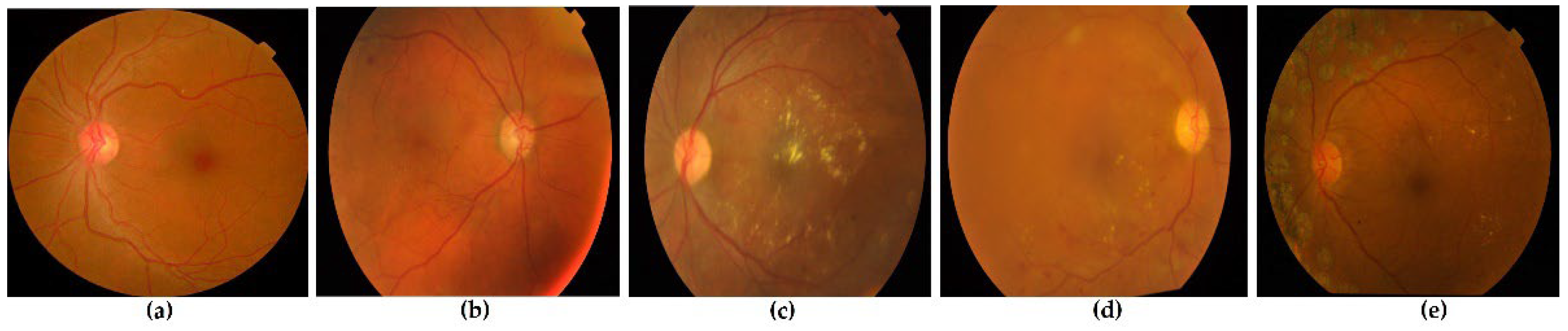
Figure 2.
The suggested study’s workflow.
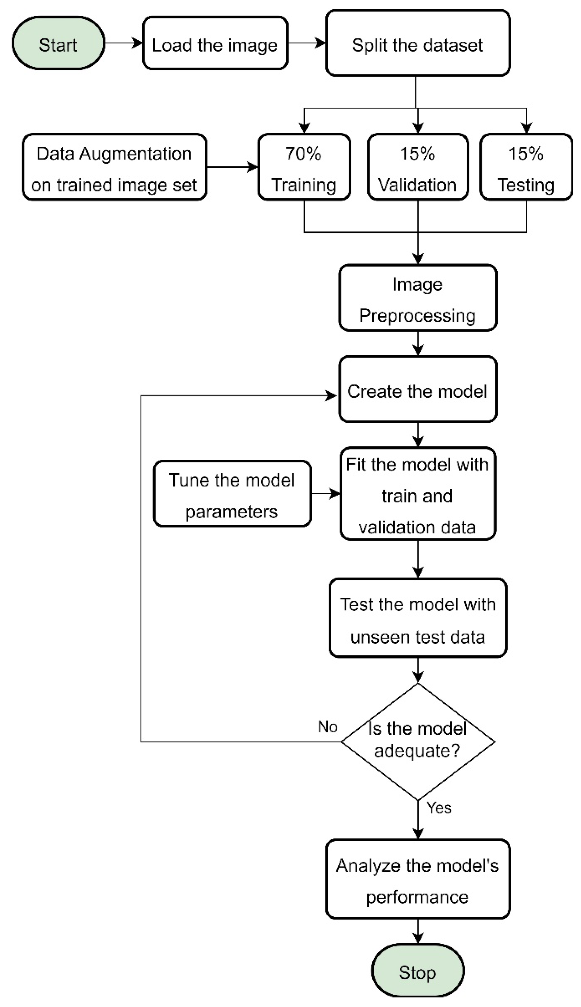
Figure 3.
Example of an augmented image from a random image in training data. From left to right: the original image, followed by a horizontally flipped image, height-shifted image, width-shifted image, and rotated image.
Figure 3.
Example of an augmented image from a random image in training data. From left to right: the original image, followed by a horizontally flipped image, height-shifted image, width-shifted image, and rotated image.
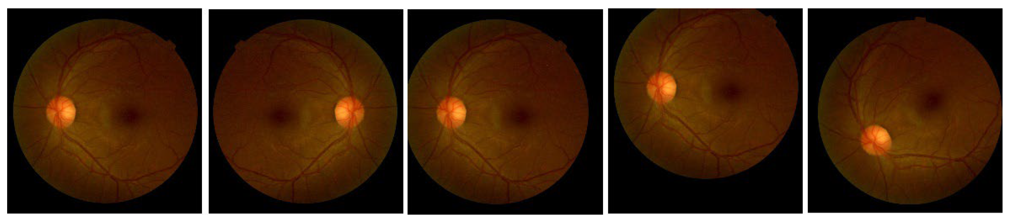
Figure 4.
The architecture of the proposed model.
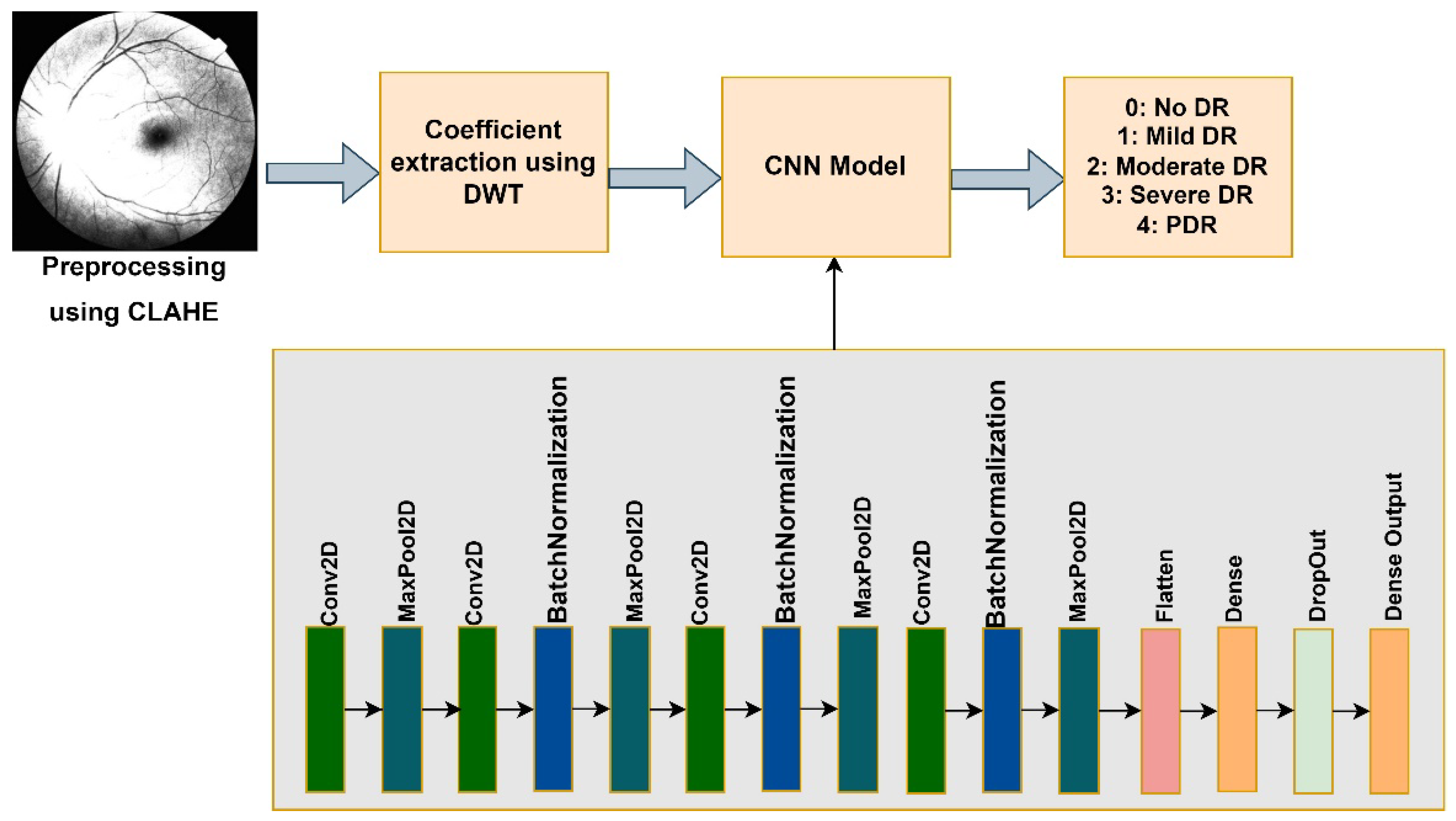
Figure 5.
The original and preprocessed image in the model. (a) raw image, (b) CLAHE preprocessed image, (c) sample of Approximation coefficients from DWT preprocessing.
Figure 5.
The original and preprocessed image in the model. (a) raw image, (b) CLAHE preprocessed image, (c) sample of Approximation coefficients from DWT preprocessing.
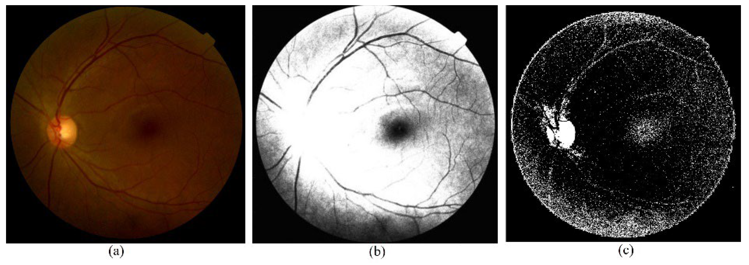
Figure 6.
The accuracy plot of training and validation data. (a) Adam optimizer, (b) RMSProp optimizer, (c) SGD optimizer, (d) Adagrad optimizer, (e) Adamax optimizer.
Figure 6.
The accuracy plot of training and validation data. (a) Adam optimizer, (b) RMSProp optimizer, (c) SGD optimizer, (d) Adagrad optimizer, (e) Adamax optimizer.
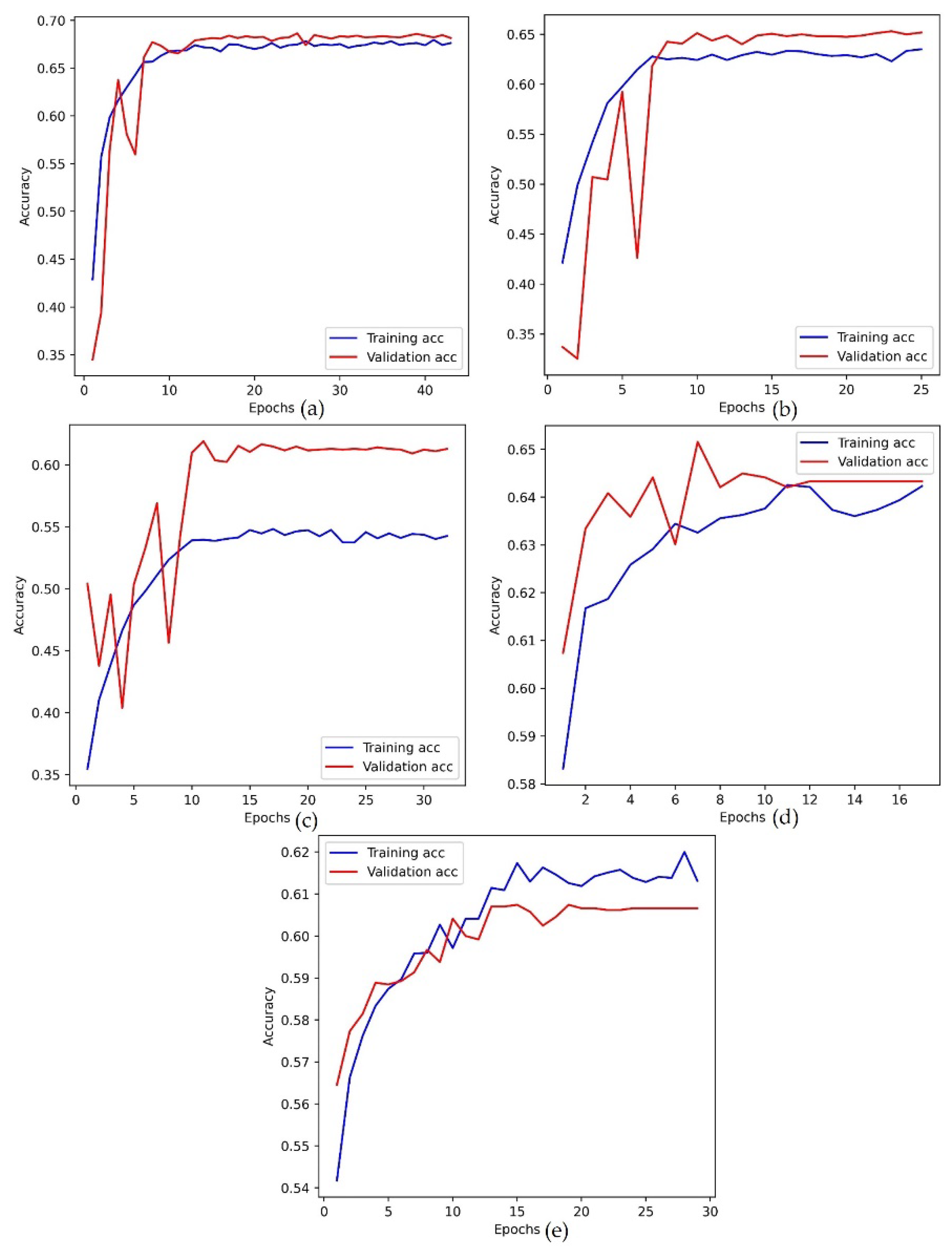
Figure 7.
The loss plot of training and validation data. (a) Adam optimizer, (b) RMSProp optimizer, (c) SGD optimizer, (d) Adagrad optimizer, (e) Adamax optimizer.
Figure 7.
The loss plot of training and validation data. (a) Adam optimizer, (b) RMSProp optimizer, (c) SGD optimizer, (d) Adagrad optimizer, (e) Adamax optimizer.
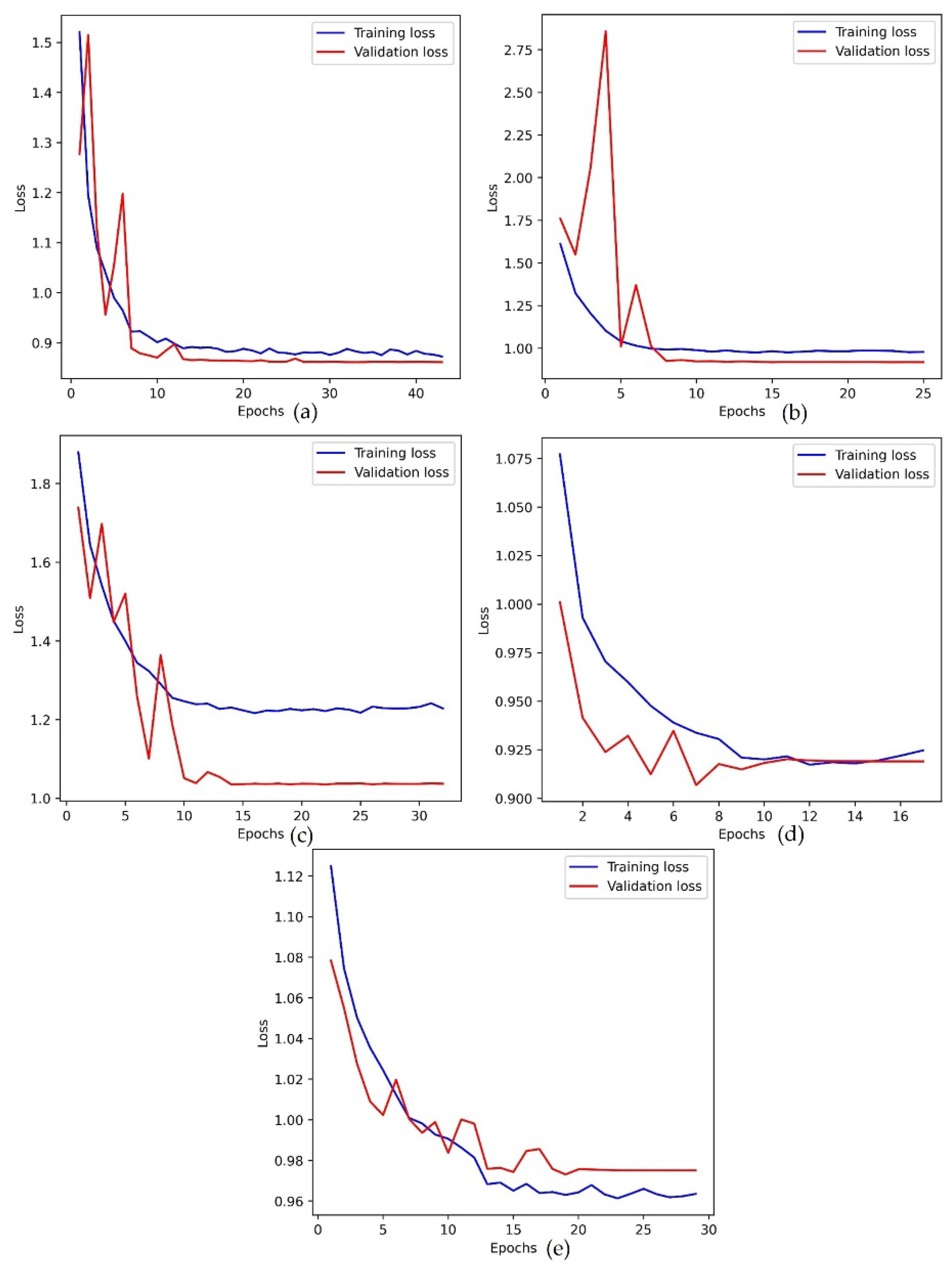
Figure 8.
The comparison of the proposed model’s performance with the test dataset.
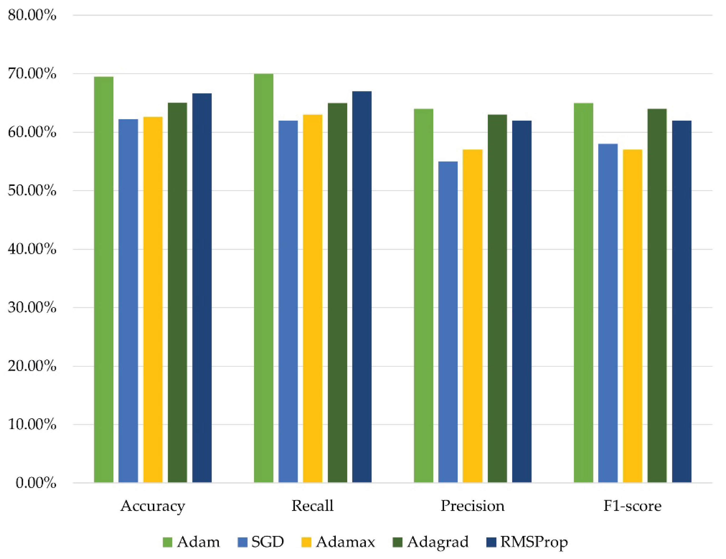

Table 1.
Inference from the previous studies related to the classification of DR stages.
| Reference | Model | Dataset | Advantage | Disadvantage |
|---|---|---|---|---|
| [19] | DenseNet121 | APTOS, EyePACS, ODIR | Able to classify based on different datasets. | The stage of DR is not detected. |
| [51] | CNN | Kaggle | The model achieves an accuracy of 89%. | The model needs to be tested on different datasets. |
| [52] | VGG16 | IDRiD | The model was capable of detecting different stages of DR. | The model was tested on very few images. |
| [53] | Vision Transformer | DDR, IDRiD | The model was capable of detecting different stages of DR. | The model has a class imbalance problem and tests on a few images. |
| [54] | ResNext, DenseNet | APTOS | The model classifies the DR with high performance. | The model has a class imbalance problem and tests on a single dataset. |
| [55] | Capsule network | Messidor | The model detects the stages of DR. | Only four stages are detected and tested only on a single dataset. |
| [56] | InceptionV3, Resnet50, CNN | Messidor, IDRiD | The model classifies the DR with high performance. | The features are extracted using only two pretrained models. |
| [35] | U-Net | APTOS, Messidor | The model segments and detects the stages of DR. | Only four stages are detected, and parameter tuning can be performed. |
| [57] | EfficientNet, VGG16, InceptionV3 | APTOS | The model classifies DR after CLAHE preprocessing. | The stage of DR is not detected, and only a single dataset is evaluated. |
| [58] | InceptionV3 | APTOS | The model classifies DR stages after CLAHE preprocessing. | Only a single dataset and model are evaluated. |
| [59] | Swin Transformer | APTOS | The model classifies DR with high performance. | The stage of DR is not detected, and the model can be tuned with more datasets. |
| [43] | VGG16 | APTOS, Mauritius | The model detects the stages of DR. | The model needs to be tuned for moderate and proliferative DR. |
| [45] | Wavlet with Swin Transformer | APTOS | The classification accuracy was improved. | The study only utilized a single image set for testing the model. |
| [48] | DWT with KNN, SVM | Messidor | The model classifies the normal, and DR images perfectly. | The stage of DR is not detected, and the dataset contains fewer samples. |
Table 2.
The count of each class in training, validating, and testing datasets.
| Dataset | Class 0 | Class 1 | Class 2 | Class 3 | Class 4 |
|---|---|---|---|---|---|
| Training | 5824 | 722 | 3953 | 310 | 873 |
| Validation | 1028 | 127 | 698 | 55 | 154 |
| Testing | 1210 | 150 | 821 | 64 | 181 |
Table 3.
The training parameter of the model.
| Parameter | Value |
|---|---|
| Image size | 150 |
| Initial Learning rate | 0.001 |
| Optimizer | Adam, SGD, Adamax, Adagrad, RMSProp |
| Loss function | SparseCategoricalEntropy |
| Epoch | 70 |
| Batch Size | 32 |
Table 4.
The validation accuracy of the APTOS-DDR dataset.
| Optimizers | Accuracy | Loss |
|---|---|---|
| Adam | 68.77% | 0.8432 |
| SGD | 61.29% | 1.0354 |
| Adamax | 60.74% | 0.9731 |
| Adagrad | 64.95% | 0.9069 |
| RMSProp | 65.06% | 0.9185 |
Table 5.
The test accuracy result of all optimizers.
| Optimizer | Accuracy | Recall | Precision | F1-score | Loss |
|---|---|---|---|---|---|
| Adam | 69.51% | 0.70 | 0.64 | 0.65 | 0.8215 |
| SGD | 62.21% | 0.62 | 0.55 | 0.58 | 1.0032 |
| Adamax | 62.61% | 0.63 | 0.57 | 0.57 | 0.9573 |
| Adagrad | 65.05% | 0.65 | 0.63 | 0.64 | 0.8988 |
| RMSProp | 66.67% | 0.67 | 0.62 | 0.62 | 0.8906 |
Table 6.
The AUC score of the test result.
| Optimizer | AUC |
|---|---|
| Adam | 0.8153 |
| SGD | 0.7253 |
| Adamax | 0.7783 |
| Adagrad | 0.7885 |
| RMSProp | 0.7772 |
Table 7.
Comparison of the proposed study with previous studies.
| Reference | Year | Model | Class type | Dataset | Accuracy | F1-score | AUC |
|---|---|---|---|---|---|---|---|
| [48] | 2018 | KNN, DWT | Binary | Messidor | 98.16% | - | - |
| [69] | 2022 | CNN | 5-class | DDR | 66.68% | - | - |
| [53] | 2023 | Vision Transformer | 6-class | DDR | 91.54% | 0.67 | - |
| [45] | 2024 | Swin Transformer, DWT | 5-class | APTOS | 86.00% | - | - |
| Proposed model | CNN with CLAHE, DWT | 5-class | APTOS+DDR | 69.51% | 0.65 | 0.81 | |
Disclaimer/Publisher’s Note: The statements, opinions and data contained in all publications are solely those of the individual author(s) and contributor(s) and not of MDPI and/or the editor(s). MDPI and/or the editor(s) disclaim responsibility for any injury to people or property resulting from any ideas, methods, instructions or products referred to in the content. |
© 2024 by the authors. Licensee MDPI, Basel, Switzerland. This article is an open access article distributed under the terms and conditions of the Creative Commons Attribution (CC BY) license (http://creativecommons.org/licenses/by/4.0/).
Copyright: This open access article is published under a Creative Commons CC BY 4.0 license, which permit the free download, distribution, and reuse, provided that the author and preprint are cited in any reuse.


