
Submitted:
01 March 2024
Posted:
01 March 2024
You are already at the latest version
Abstract
The quality prediction of quaternary structure models of a protein complex, in the absence
of its true structure, is known as the Estimation of Model Accuracy (EMA). EMA is useful for
ranking predicted protein complex structures and using them appropriately in biomedical research,
such as protein-protein interaction studies, protein design, and drug discovery. With the advent
of more accurate protein complex (multimer) prediction tools, such as AlphaFold2-Multimer and
ESMFold, the estimation of the accuracy of protein complex structures has attracted increasing
attention. Many deep learning methods have been developed to tackle this problem; however,
there is a noticeable absence of a comprehensive overview of these methods to facilitate future
development. Addressing this gap, we present a review of deep learning EMA methods for protein
complex structures developed in the past several years, analyzing their methodologies and impacts.
We also provide a prospective summary of some potential new developments for further improving
the accuracy of the EMA methods.
Keywords:
Protein quality assessment
; estimation of model accuracy
; deep learning
; protein complex
; protein quaternary structure
1. Introduction
Proteins interact to form complexes that carry out important biological functions. Therefore, obtaining the quaternary structure of a protein complex is crucial for elucidating how proteins interact. This information proves useful in addressing various biological research problems that require protein-protein interaction (PPI) details, such as drug discovery [1,2,3] and protein design [4,5].
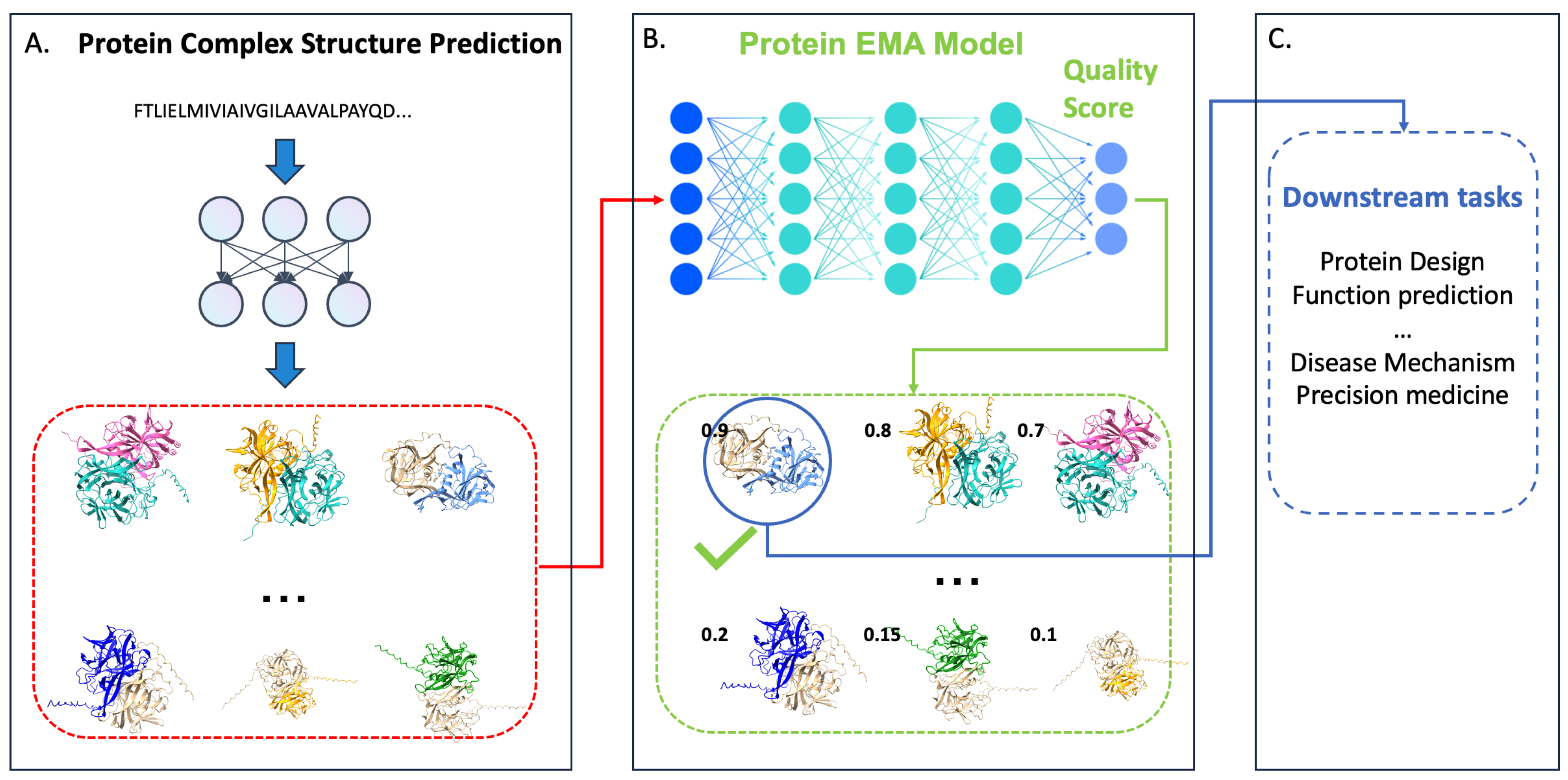
Typically, high-resolution structures of protein complexes are determined with methods such as X-ray crystallography and cryo-electron microscopy (cryo-EM). However, these low-throughput methods can only solve a small portion of protein complex structures. As a result, computational protein complex (multimer) prediction methods have gained significant attention in the scientific community. Recently, some advanced deep learning protein multimer predictors, such as AlphaFold-Multimer [6], have substantially accelerated the process of predicting protein complex structures. These tools initially generate a large number of protein-complex decoys. Then, the quality of all the predicted structures (decoys) needs to be assessed (predicted) by a quality evaluation method, which is not aware of the native structure of the protein complex, that ultimately selects the decoy with the highest score. Typically, this phase is referred to as the estimation of model accuracy (EMA), protein quality assessment (QA), or model scoring problem. Figure 1 illustrates such a protein complex structure prediction and quality evaluation process. As seen, after an EMA method selects the highest-ranked decoy, that decoy is passed to downstream application tasks.
Numerous methods have been developed to address the challenging problem of estimating the accuracy of protein complex structures [7,8,9,10,11,12,13]. Commonly, EMA methods can be categorized into three types of approaches: physical energy-based [12], statistical potential-based [7,8], and machine learning-based. Physical energy-based methods typically use scoring functions consisting of a weighted linear combination of various physical energetic terms. Due to their lower computational complexity, these models are frequently employed in numerous docking methods [14,15,16]. Statistical potential-based methods convert the distribution of distance-relevant or irrelevant pairwise contacts at atom or residue level into statistical potentials [8]. Machine learning or deep learning-based methods [11,13,17,18,19,20,21,22,23,24,25,26,27,28,29,30,31] generally use features to represent a protein quaternary structure, which are then used to predict the structures quality scores. Similar to the protein tertiary structure EMA task, quaternary structure EMA methods can also be classified into multi-model [23,32] and single-model approaches [24,25]. Multi-model methods [22,23] yield a relative score for each predicted protein-complex decoy in a model pool, leveraging the similarity between structural models to assess quality. In contrast, single-model methods consider only one decoy and assign an absolute quality score to it, independent of comparisons with other decoys.
In this review, we will concentrate on the deep learning-based protein quaternary structure EMA methods developed in the last five years. The structure of this review is as follows: First, we will introduce the metrics for evaluating the quality of protein complex structures and the performance of EMA methods. Then a discussion on prevalent methods for representing protein complex structures for EMA and common datasets used to train and test EMA methods. Subsequently, we explore the recent deep learning EMA methods, categorized by their technical approaches. Finally, we conclude the review with a perspective on future trends in the development and enhancement of protein complex structure EMA methods.
2. Metrics for Evaluating the Quality of Protein Complex Structures and the Performance of EMA Methods
CASP (Critical Assessment of Techniques for Protein Structure Prediction) and CAPRI (Critical Assessment of PRedicted Interactions) are two worldwide experiments that rigorously test computational methods of predicting protein complex structures and estimate their accuracy. The latest competitions [33] offer widely accepted measures for assessing the overall (global) structural quality, interface quality, and local structural quality of predicted complex structures with respect to their true structures. As well as evaluating the performance of EMA methods of estimating/predicting the accuracy of predicted complex structures as discussed below.
2.1. Global Structural Quality Evaluation of Protein Complex Structure
CASP uses oligo-GDT-TS [34] and TMscore [35] to evaluate the global structural quality of a predicted complex structure.
oligo-GDT-TS: Similar to the GDT-TS (Global Distance Test Total Score) [34] used to evaluate a predicted tertiary structure, oligo-GDT-TS extends the calculation to the global structural similarity score of the predicted complex structures with respect to the true structure. This is done using equation 1 with different distance thresholds (e.g., 8Å, 4Å, 2Å, 1Å), where denotes the percentage of residues in the model that are within a distance threshold n to their counterparts in the true structure after the predicted structure and the true structure are superimposed.
TMscore: Unlike oligo-GDT-TS, the Template Modeling score (TMscore) rescales residue-wise modeling errors, eliminating the dependency on protein size. TMscore is calculated using equation 2, where is the length of a target complex structure, is the number of the aligned residue pairs, is the distance between the atoms of the pair of residues from the two structures (e.g., a predicted target complex structure and the corresponding true structure), and is calculated by equation 3 according to the length of the predicted protein complex.
2.2. Interface Quality Evaluation of Protein Complex Structure
The interface quality measurement is meant to evaluate the similarity between the structure of the residues in the interaction interface of a predicted protein complex structure and the structure of their counterparts in the true structure. DockQ score [36] is a widely used metric to measure interface quality and is calculated based on three complementary measurements: , , and .
is the fraction of native contacts in the protein-protein interfaces in the true complex structure preserved in the predicted protein complex structure. Protein-protein interface residues are determined by whether the distance between any two heavy atoms of two residues from two different protein chains is less than 5Å. This fraction, denoted as , ranges from 0 to 1, with a higher value indicating a greater preservation of native contacts in the predicted complex structure.
, ligand root mean square deviation (RMSD) is defined as the RMSD of the backbone of a chain of the predicted complex structure called ligand (usually the shorter chain) after the structure of another chain called the receptor (usually longer chain) is superimposed with that of the true structure. The larger the value, the worse the predicted complex structure.
, interface root mean square deviation is the root mean squared deviation between the residues in the interface region of a predicted complex structure and the true structure. The larger the value, the worse the predicted complex structure is in comparison with the true structure.
DockQ, in the range [0, 1], is the average of , scaled , and scaled , calculated according to equation 4. The scaled value of and are determined by equation 5 with two thresholds ( and ), respectively. The threshold values for (8.5Å) and (1.5Å) are selected through a grid search to optimize the F1-score for classifying predicted protein complex structures in a dataset into the four quality classes (Incorrect, Acceptable, Medium and High) as commonly used in the CAPRI competition. Additionally, these four quality classes can be further grouped into two main classes: incorrect and correct.
In addition to the DockQ score, QS-score [37] is also used to evaluate the interface quality of complex structures. QS-score, expressed by the weighted fraction of shared interface contacts (e.g., residue-residue pairs with distance < 12Å), is another robust continuous score used to measure the interface quality of a predicted complex structure. It is calculated by equation 6, where and denote the distance between two residues in a contact in protein structure A (e.g., predicted structure) and B (e.g., true structure) respectively. The weighting function is calculated with equation 7, which is the probability of a side-chain interaction between two residues given their distance. A higher QS-score indicates a higher similarity between compared interfaces.
CAD-score [38] is another metric to evaluate interface quality. Let G be the set of the residue pairs with nonzero contact areas in a predicted complex or true complex structure. and are the contact areas for residue pair in the true structure and predicted structure respectively. The CAD score is calculated with equation 8, where the is calculated by equation 9 and is calculated by equation 10. The higher the CAD-score, the better the interface quality is.
2.3. Local Structural Quality Evaluation of Protein Complex Structure
The local structural quality of the predicted protein complex structure, i.e. the quality of the predicted position of each residue or each atom in a predicted complex structure, is often evaluated by Local Distance Difference Test (lDDT) score [39].
lDDT quantifies the degree to which a protein structure accurately replicates the environment found in the true structure. For each atom in the true structure, the nearby atoms from different residues are identified by a distance threshold. Then the percentage of the distances between one atom and other atoms in the true structure that are preserved as the predicted structure is calculated. This atom-level lDDT score is the average of the fraction calculated at 0.5Å, 1Å, 2Å, and 4Å distance thresholds considering all the atoms. In contrast, the residue-level lDDT score is calculated on the atoms only.
2.4. Metrics of Evaluating Protein Complex Structure EMA
EMA methods are developed to predict the quality score of predicted protein complex structures in the absence of true complex structures. Their performance is evaluated by comparing predicted quality scores with true quality scores, measured by metrics such as those in Sections 2.1-3. Below are some commonly used measures for evaluating the performance of EMA methods.
Correlation: The Pearson/Spearman correlation between the true and predicted quality scores of an EMA method.
MSE and MAE: Mean squared error (MSE) and Mean absolute error (MAE) between the real and the predicted quality scores of an EMA method.
Ranking loss: The difference between the quality of the actual best structure and the quality of the no. 1 ranked structure which is selected according to quality scores predicted by the EMA method. The smaller the loss, the better the ranking is.
Success rate (SSR): The percentage of near-native structures among the top n ranked structures selected by the EMA method.
Hit rate (HR): The fraction of near-native structures among the top n ranked structures, divided by the number of all near-native structures in the structure pool.
3. Learning the Representation of Protein Complex Structure
3.1. Protein Complex Structure Representation
Deep learning EMA methods take a predicted complex structure as input and predict its quality score. Unlike a vector of numbers that can be directly used as input for deep learning methods, a predicted complex structure consists of a set of atoms. This requires their x, y, and z coordinates to be converted into a representation that can be understood and processed by deep learning methods. Consequently, many different representations for protein complex structures have been developed. iScore [13] utilizes a graph random walk method to construct graph kernel matrices for a given protein complex structure, while CoDES [40] extracts a set of physicochemical and statistical potential features of protein complex structures. Both methods transform protein structures into tableau data that machine learning methods can use.
Dove [17] and TRScore [41] employ a fixed-size 3D grid to encode protein complex structures for model quality classification. PointDE [42] creates a point cloud to represent the protein interaction interface in protein complex structures to assess their quality.
More recently, several methods [20,24,27,28,30,31,43,44,45,46,47,48,49] have used graphs to represent protein complex structures. Compared to other forms, graph structures offer several advantages: 1) they can effectively represent residue-residue or atom-atom interactions, with the capacity to easily assign chemical, physical, biological, and artificial features to the nodes and edges in the graph; 2) graph representations can scale to match protein structures of various complexity and size; and 3) they are particularly suitable for some deep learning algorithms such as graph neural networks while requiring fewer computational resources than 2D and 3D grid representations. Below is a brief description of various graph neural networks used to learn the representation of protein complex structures.
3.2. Graph Neural Network
Graph neural networks (GNNs) are specifically designed to process graph-structured data. As a result, when representing protein complex structures as graph structures, GNNs naturally lend themselves to addressing protein complex EMA challenges. Here we provide a concise overview of three common GNN architectures: Graph Convolutional Networks (GCNs) [50], Graph Attention Networks (GATs) [51], and Graph Transformers (GTs) [52]. These architectures form the backbone of numerous protein complex EMA methodologies. The Main Techniques column in Table 2 summarizes the deep learning architectures used by all methods reviewed in this survey, many of which are based on GNNs.
3.2.1. Graph Convolutional Neural Network
Graph convolutional neural network (GCN) is a type of neural network that applies the capabilities of a convolutional neural network to a graph data structure. They provide a particular advantage in making complex neural networks understandable by utilizing the layer-wise propagation equation 11 for a specific graph-based neural network model :
This expression outlines how each layer processes information. represents the adjacency matrix of the undirected graph G with the addition of the identity matrix adding self-connections to each node in the graph. is the diagonal elements of a degree matrix where i is the i-th diagonal element of said matrix. is computed with the sum of the elements of each row within where i and j represent the element in the i-th row and j-th column of the matrix. Within the GCN, each layer has its own trainable weight matrix . The activation function is applied to the results of the matrix operations. is a matrix that represents node features in the lth layer of the GCN where equals the initial layer X and in each layer is updated using the defined operations.
3.2.2. Graph Attention Neural Network
Graph attention neural networks (GAT) receive an input of nodes h = {, ,⋯,}, where N is the number of nodes and F is the number of features in each node. To obtain initial transformation features, for each input node, it applies a shared linear transformation, parameterized by the weight matrix where to each node. A self-attention mechanism then computes , indicating the importance of node j’s features to node i using the equation . In this formula, a represents a weight vector that parameterizes the attention mechanism. Here graph structure is incorporated by only computing for nodes where is some neighborhood of node i in the graph. To improve the comparability across nodes, is normalized by the softmax function (equation 12) across all the neighbors of node i, resulting in an attention weight .
Finally, the layer outputs an updated node features h = {, ,⋯,}, with a potentially different number of features , from the weighted sum of the features of the neighbors of each node.
3.2.3. Graph Transformer Neural Network
The Graph Transformer (GT) neural network adapts the transformer model [53] from graph data processing to update both node and edge features, which is different from GAT above which only updates node features. A graph G, characterized by initial node features and edge features , is input into the Graph Transformer layer for message passing and feature updating. Initially, the Graph Transformer layer computes the attention scores by utilizing both and . Subsequently, it derives updated intermediate node features and edge features based on these attention scores. The outputs are then passed to a feed-forward network which is proceeded and succeeded by residual connections and normalization layers, leaving the final output the updated node feature and edge feature .
4. Datasets for Training and Test Protein Complex EMA Methods
Training, validation, and testing constitute critical stages in the development of deep learning methods. The quantity and quality of the training and test data are critical for constructing high-performing deep learning methods. Table 1 enumerates some commonly used datasets for training, validating, and testing protein complex structure EMA methods.

Table 1.
The six common protein complex benchmark datasets. All the datasets except Docking Benchmark contain both true and predicted structures. The Docking Benchmark dataset includes only true (native) structures.
Table 1.
The six common protein complex benchmark datasets. All the datasets except Docking Benchmark contain both true and predicted structures. The Docking Benchmark dataset includes only true (native) structures.
| Data Sources | Number of Targets/Structures | Source |
|---|---|---|
| DockGround | 61/6100 | Link |
| Docking Benchmark | 230/* | Link |
| PPI4DOCK | 1417/54000 | Link |
| CARPI set | 15/19013 | Link |
| CASP15 | 38/9930 | Link |
| DBM55-AF2 | 15/450 | Link |
DockGroup set [54] provides two docking decoy sets for the EMA benchmark, which are associated with 61 unbound complex targets. Each target has 100 decoy models, including at least one near-native () decoy generated by a protein docking tool GARMM-X [55,56].
The Docking Benchmark set (BM set) is a successful protein-protein scoring benchmark dataset series, with the first DBM set published in 2003 [57] being named DBM1.0. Each later BM set version was built on top of the previous version by adding new targets. The latest version, DBM5.5 [58], contains 230 complex targets, several decoys predicted for them, and the quality scores (labels) of the decoys.
The PPI4DOCK docking set [59] contains 1417 non-redundant docking targets, and also provides 54000 decoys generated by ZDock 3.0.2 [60]. A CARPI set [61] consists of 15 published CAPRI targets, a total of 19013 decoys generated by 47 different predictor groups. About of decoys are of acceptable or higher quality (based on CAPRI standard). The CASP15 dataset has 38 complex targets with each target containing around 250 decoys generated by different structure prediction teams. DBM55-AF2 [24], contains 15 targets with a total of 300 decoys generated by AlphaFold-Multimer. DockGroud set, PPI4DOCK, CAPRI set, CASP15, and DBM55-AF2 provide both decoys and native structures for each target. By calculating the quality metric of each decoy with respect to the native (true) structure as labels, decoys can be used for training and testing deep learning models.
For accurately assessing a deep learning method’s performance, the redundancy between the training and test datasets should be removed. Usually, a target is not included in a test set when its sequence has 30% or higher sequence identity with any protein target in training and validation datasets.
It is worth noting that the size of most datasets above is small and their decoy models were generated by traditional docking methods instead of the state-of-the-art protein complex structure prediction methods such as AlphaFold-Multimer, which may not be sufficient to train large deep learning methods. Therefore, most recent deep learning EMA methods [24,26,27,28,48] have used their own custom datasets for training. For example, DProQA applied AlphaFold2 [62] and AlphaFold2-Multimer [63] to generate complex structures for training. VoroIF-GNN [21] collected 1567 heterodimers structures and used FTDock[64] and FASPR [65] to generate decoys for them for training.
5. Deep Learning-based EMA Methods for Protein Complex Structure
In this section, we review the deep learning-based protein complex structure EMA methods developed within the last 5 years. Table 2, Table 3 and Table 4 list all methods’ summary information, including released date, main techniques, predictions, representation (atom/residue) level, single/multi-model method designation, input features, training dataset, testing dataset, and source code’s URL.
Table 2.
Summary of EMA methods for protein complex structures (Part 1). *: Paper accepted time.
| Name | Year* | Main Techniques |
Prediction | Representation Level |
Single-/ Multi-model |
|---|---|---|---|---|---|
| PAUL [44] | 2020 | Equivariant-GCN | iRMSD | Atom | Single |
| DOVE [17] | 2020 | 3D-CNN | The probability of an input decoy has a acceptable quality or not | Atom | Single |
| EGCN [12] | 2020 | GCN | iRMSD | Residue | Single |
| GNN_DOVE [18] | 2021 | GAT | The probability of an input decoy has a acceptable quality or not | Atom | Single |
| DGANN [66] | 2021 | GAT | The probability of an input decoy is near-native or not | Residue | Single |
| Trscore [41] | 2022 | 3D-CNN | The probability of an input decoy is near-native or not | Atom | Single |
| DeepRank_GNN [25] | 2022 | GNN | f-nat (fraction of native contacts) | Residue | Single |
| VoroIF-GNN [67] | 2023 | GAT | CAD score | Atom | Single |
| DeepUMQA3 [27,45] | 2023 | 2D-CNN | lDDT | Residue | Single |
| DProQA [24] | 2023 | GT | DockQ | Residue | Single |
| G-RANK [30] | 2023 | GVP | f-nat (fraction of native contacts) | Atom | Single |
| PIQLE [31] | 2023 | GAT | Interface score, Fold score, Residue score | Residue | Single |
| GraphGPSM [46] | 2023 | EGNN | TM-Score | Residue | Single |
| GraphCPLMQA [47] | 2023 | GT+EGNN+2DCNN | lDDT | Residue | Single |
| PointDE [42] | 2023 | Point cloud network | The probability of an input decoy is near-native or not | Atom | Single |
| ComplexQA [48] | 2023 | GCN | Interface residue score | Residue | Single |
| GCPNet-EMA [49] | 2024 | GCP | lDDT | Residue | Single |
Table 3.
Summary of EMA methods for protein complex structures (Part 2)
| Name | Features |
|---|---|
| PAUL | Atomic positions and types |
| DOVE | Contact potentials, GOAP, ITScore |
| EGCN | Node features: side-chain pseudo atom’s charge, non-bonded radii, and distance-to-Ca, solvent accessible surface area(SASA). Edge features: Atom distance features |
| GNN_DOVE | Node features: atom physicochemical proprieties of atoms. Edge features: covalent bonds, atom distance. |
| DGANN | Node features: physical-chemical properties, PSSM, Information Content |
| Trscore | Atoms’ physicochemical features |
| DeepRank_GNN | Node features: residue type, residue charge, residue polarity, buried surface area, PSSM; conservation score, information content, residue depth, residue half sphere exposure. Edge feature: residue distance |
| VoroIF-GNN | Node features: contact surface areas, contact-solvent border length, sum of inter-contact border lengths; contact type-dependent descriptors. Edge feature: Inter-contact border length |
| DeepUMQA3 | Ultrafast Shape Recognition (USR), residue voxelization, inter-residue distance and orientations, amino acid properties; level of intra-monomer: sequence embedding, secondary structure, energy terms; inter-monomer level: attention map of the inter-monomer paired sequence, inter-monomer USR |
| DProQA | Node features: residue type, secondary structure type, relative accessible surface area, torsion angles, node positional encoding. Edge features: Three types of distance, edge positional encoding, contact indicator, permutation-invariant chain encoding |
| G-RANK | Node features: atom types; Edge features: edge direction, edge length |
| PIQLE | Node features: residue encoding, relative residue positioning, secondary structure, SASA, torsion angles, number of effective sequences (Neff). Edge features: multimeric interaction distance, multimeric interaction orientation |
| GraphGPSM | USR, residue voxelization, inter-residue distance and orientations, amino acid properties; level of intra-monomer: sequence embedding, secondary structure, energy terms; inter-monomer level: attention map of the inter-monomer, paired sequence, inter-monomer USR, Ca coordinates |
| GraphCPLMQA | MSA embedding, sequence embedding, structure embedding, triangular location and residue-level contact order, relative position encoding, dihedral and planar angles, voxelization and distance map, Meiler, Blosum62 and DSSP |
| PointDE | Atomic type, residue types and coordinate, chain identity |
| ComplexQA | Sequence features, three-dimensional structural and chemical features |
| GCPNet-EMA | Node features: residue type, positional encoding, virtual dihedral and bond Angles over the trace, residue backbone dihedral angles; Residue-wise ESM Embeddings, residue-wise AlphaFold 2 plDDT, residue-sequential forward and backward vectors; Edge features: Euclidean Distance between connected atoms, directional vector between connected atoms |
Table 4.
Summary of EMA methods for protein complex structures (Part 3)
| Name | Training Data | Testing data | Source |
|---|---|---|---|
| PAUL | DBM4 | DBM5, PPI4DOCK | NA |
| DOVE | DBM4 | DockGround | https://kiharalab.org/dove/ |
| EGCN | DBM4 | CAPRI | https://github.com/Shen-Lab/EGCN |
| GNN_DOVE | Dockground, DBM4 | CAPRI | https://github.com/kiharalab/GNN_DOVE |
| DGANN | DBM4 | DBM5.5 | https://github.com/coffee19850519/PPDocking/tree/master |
| Trscore | DBM4 | DBM5 | https://github.com/BioinformaticsCSU/TRScore |
| DeepRank_GNN | DBM5 | CAPRI | https://github.com/DeepRank/Deeprank-GNN |
| VoroIF-GNN | Custom set | Custom set | https://www.voronota.com/expansion_js/ |
| DeepUMQA3 | Custom set | Custom set | http://zhanglab-bioinf.com/DeepUMQA/ |
| DProQA | Dockground, DBM5.5, Custom Dataset | Custom Dataset | https://github.com/jianlin-cheng/DProQA/tree/main |
| G-RANK | DBM5 | CAPRI | https://github.com/ha01994/grank |
| PIQLE | Dockground v2 | Dockground v1 | https://github.com/Bhattacharya-Lab/PIQLE |
| GraphGPSM | Custom set | CASP15 | http://zhanglab-bioinf.com/GraphGPSM/ |
| GraphCPLMQA | Custom set | CASP15 | http://zhanglab-bioinf.com/GraphCPLMQA/ |
| PointDE | DOCKGROUND | CAPRI, Custom Dataset | https://github.com/AI-ProteinGroup/PointDE |
| ComplexQA | DockGround, DBM5, Custom Dataset | Custom set | https://github.com/Cao-Labs/ComplexQA/tree/main |
| CGPNet-EMA | Custom set | CASP15, Custom set | https://github.com/BioinfoMachineLearning/GCPNet-EMA |
TRScore [41] employs a 3D CNN architecture, adapted from a ResNet-inspired VGG [68,69] architecture with structural re-parameterization technique (RepVGG), to predict the likelihood of a near-native model for an input 3D complex structure. When provided with an input 3D structure, a 3D grid with shape and 2Å grid spacing is constructed after voxelizing the cube that is placed on the centroid of the protein-protein interface. Each voxel in the grid is then assigned a 19-dimensional vector feature representing the counts of atoms of different types within the voxel. Evaluated on the BM5 dataset, DockGround unbound decoy set, and CAPRI decoy set, TRScore can obtain a performance comparable to or better than DOVE [17], ZRANK [70], ZRANK2 [71] and IRAD [10] in terms of success rate and hit rate.
DOVE [17] applies two knowledge-based statistical potential values, GOAP [72] and ITScore [9], as the description of input decoy and also represents the position of carbon, oxygen, nitrogen, and other atoms at the interface. Concatenated and reshaped these features as the fixed cube shape () for a 3D CNN model to predict the probability that an input protein complex structure has an acceptable model quality based on the CAPRI standard. The DOVE is trained and validated on the BM4.0 dataset [73] and tested on the DockGround set [54]. Because it uses a fixed-size cube as input, DOVE faces the difficulty of accurately capturing the protein interface of large-size protein complex structures. Also, 3D-CNN is computationally expensive for modeling. To address these issues, the GNN-DOVE [18] is proposed. GNN-DOVE extracts the interface region of the protein complex and then reconstructs a graph with/without inter-molecular interactions to represent it as input. It then predicts a probability that the input protein complex has a CAPRI-acceptable quality. GNN-DOVE was trained on the DockGround and DBM4 set. For a fair comparison with DOVE, DOVE was also retrained on the same dataset as GNN-DOVE. On the CAPRI set [61], GNN-DOVE shows a higher performance in terms of hit rate.
PAUL [44] is an end-to-end protein complex scoring system. PAUL does not use any pre-calculated statistical or physical terms as the input feature for the neural network. PUAL instead uses rotation-equivariant neural networks with three hierarchical structures to represent protein-protein complex atoms’ positions and types. PAUL consists of two models with the same architecture: the first one is a classification model (for ranking purposes) to predict if a decoy has an acceptable quality (i.e., < 10Å), and the second one is the regression model (for model quality assessment purpose) to directly predict the LRMSD. PAUL’s training dataset is BM4.0 and evaluated on BM5.0 (excluding the BM4.0 part) and PPI4DOCK set. Because of PAUL’s ranking ability, it is sometimes used to enhance other model scoring methods’ ranking ability. PAULSOAP-PP and PAULZRANK for example use PAUL to filter out sub-optimal decoys first and then rank the remaining decoys using SOAP-PP or ZRANK), which perform better than using SOAP-PP and ZRANK alone in both benchmark datasets.
ECGN [12] utilizes two identical GNNs with different parameters to represent intra- and inter-molecular residue-residue contacts in a protein complex structure to predict its binding energy. The energy term is calculated from the interface root mean square deviation (iRMSD) of the complex structure. For both intra- and inter-molecular residue contact graphs, ECGN employs 4 node features and 11 edge features. ECGN was trained on the BM4 dataset and tested on the CAPRI targets and score_set. On the test datasets, ECGN demonstrates a better performance than a random forest-based scoring method on both the ranking task and the quality estimation task and its performance is comparable to iRAD [10].
PIQLE [31] utilizes GAT to predict a single global interface quality score from the interaction interface graph extracted from the input protein complex structure. Each graph is assigned 17 residue-level sequence- and structure-based node features and 27 multimeric geometric-based edge (interaction) features. PIQLE was trained on the DockgGround set and benchmarked on HAF2 set [24], achieving a better performance than DProQA [24], TRScore, GNN-DOVE, and DOVE.
DGANN [66] employs a deep graph attention neural network to predict the likelihood of a protein complex structure model being a near-native model. The graph for an input structure is constructed by treating residues with encoded physical-chemical properties and Position-Specific Scoring Matrix (PSSM) features as nodes, while edges are established when the minimum distance between any two atoms from two different residues is less than 5Å. Benchmarked on the BM5.5 dataset, DGANN outperformed ZDOCK, HADDOCK [74], iScore [13] and DOVE-Atom40 in terms of success rate and enrichment factor.
DeepRank_GNN [25] adapts a graph structure to represent a protein dimer structure for interface quality prediction. Similar to DGANN, the construction of the graph involves treating residues with their features (e.g., residue type, residue charge, residue polarity, and PSSM) as nodes, with edges symbolizing the contact between the residues. Different from DGANN, DeepRank_GNN builds two distinct input graphs formed by intra-chain (e.g., a minimum atomic distance less than 8.5Å) and inter-chain contacts (e.g., a minimum distance between heavy atoms less than 3Å). These graphs are then inputted into the graph neural network to predict the fraction of native contacts in the input structure. Benchmarked on the CAPRI dataset, DeepRank_GNN performed better than HADDOCK, DeepRank [75], DOVE, GNN-DOVE and iScore in terms of AUC.
DProQA [24] encodes a protein complex structure as a KNN (10 neighbors) graph and feeds it to a gated graph transformer to predict a real-valued quality score of the structure as well as a quality class that it belongs to. The graph’s node and edge features are all directly generated from the input protein complex structure without using any extra information such as multiple sequence alignments (MSAs) and residue residue co-evolutionary features extracted from MSAs. DProQA is trained and tested on the newly developed protein complex datasets in which all structural decoys were generated using AlphaFold2 and AlphaFold-Multimer. In the blind CAPSP15 experiment, DProQA is one of the top performers among all single-model methods in terms of ranking loss.
G-RANK [30] is built on top of the geometric vector perceptron–graph neural network (GVP) [76]. GVP uses directed Euclidean vectors to represent the positions of atoms of protein complex structures for downstream machine learning tasks. G-RANK uses the graph to represent the protein complex structure’s interface, with atom type as node features, and edge direction and length as edge features. Both node and edge features are embedded in a high-dimension feature space. They are then sent to GVP for updating via message passing and predicting an interface quality score .
GCPNet-EMA [49] represents a successful implementation of Geometry-Complete Perceptron (GCP) Networks [77] for the protein complex structure EMA task. Given a protein complex structure, GCPNet-EMA constructs a residue-level graph, incorporating initial node features, edge features, and frames derived from the residues’ coordinates. These features are processed through several SE(3)-equivariant GCPConv layers. Subsequently, the model employs its learned fine-tuned representations to predict the lDDT score for each residue (node). When benchmarked on the CASP15 multimer set, GCPNet-EMA demonstrates competitive performance in terms of ranking loss. Interestingly, GCPNet-EMA can be applied to predict lDDT scores for both protein quaternary structures and tertiary structures. Similarly, EnQA based on 3D-equivaraint graph neural networks [43] was originally trained on protein tertiary structures to predict per-residue lDDT scores, but can also be applied to predict the lDDT scores of protein quaternary structures by treating them as a single unit.
ComplexQA [48] designs a new graph-based neural network for predicting the local residue quality of protein complex interfaces based on the sequence and three-dimensional structure-derived features. ComplexQA first generated thousands of features and finally selected the top 300 features that had the highest Pearson correlation with the labels. Additionally, to accurately evaluate ComplexQA’s performance, a modified lDDT score - - is proposed. Compared to the original lDDT score, enlarges the default radius from 15Å to 30Å when calculating the fraction of local residue pairs. In its experiment, shows a higher correlation with DockQ score than lDDT.
VoroIF-GNN [67] (Voronoi InterFace Graph Neural Network) adapts the Voronoi tessellation of atomic balls of van der Waals radii to establish atomic contacts, which are aggregated to form residue contacts. The inter-residue contacts characterized by their attributes such as contact surface area, contact-solvent border length, sum of inter-contact border lengths, and contact-type descriptors serve as nodes in the constructed interface graph. Meanwhile, the inter-contact borders are designated as edges in this graph, which are fed to a graph neural network to predict the CAD-goodnesses derived from the CAD-score. Evaluated on the CASP15 dataset, VoroIF-GNN was the best single-model method in terms of ICS, IPS and lDDT-oligo.
PointDE [42] first extracts the interaction interface from a protein complex structure, and then converts it to an interface point cloud. To sample a fixed number of points from the initial interface points vector, PointDE proposes a new Nearest Pair Sampling approach to sample a fixed number of atom pairs on the interface. As a result, each final point cloud contains 500 closest atomic pairs. Each point has 3d coordinates and a 26-dimensional feature vector. PointeDE takes PointMLP [78] as the backbone and uses the Inter-molecular Group Mechanism (IGM) to replace the k-Nearest Neighbor (kNN) algorithm to aggregate geometric features during the grouping process. PointDE predicts the probability that a protein complex is native-like or not.
DeepUMQA3 [27,45] extract overall complex features, intra-chain (intra-monomer) features, and inter-chain (inter-monomer) features for a given complex structure. The overall features are generated by considering the whole complex structure as a single component, which contains ultrafast shape recognition (USR), voxelization expression, inter-residue distances and orientations, and amino acid properties. The sequence embedding generated by protein language model [79], secondary structure, and Rosetta energy terms [80] of each monomer are considered as the intra-chain features. The inter-chain features are composed of an attention map between the monomer sequence and inter-monomer USR. All these features are first combined and then updated by a triangular multiplication update layer, an axial attention layer, and a feed-forward layer to generate higher-level features. These higher-level features are fed to a residual neural network to predict the local residue quality score and interface residue accuracy. DeepUMQA3 ranked first in the accuracy estimation for protein complex interface residues in CASP15.
GraphGPSM [46] represents a protein complex as a residue-level graph and uses the same features of DeepUMQA3 [45] with the additional coordinates of the atoms of the input complex structure to embed the graph. The graph is then updated by the Equivalent-GNN (EGNN) to predict the global TM-score of the complex structure.
GraphCPLMQA [47] combines the protein language model-generated sequence- and structural-embedding features, triangular location, reside-level contact order, and physicochemical properties of protein complex structure as the initial features, which are used by a graph neural network-based encoding module to generate high-level features. The high-level features are used by a CNN-based decoding module to predict the residual-level local quality score.
6. Future Work
Significant progress has been made in estimating the accuracy of protein complex structures in the last several areas discussed. Despite this, few methods can consistently estimate the accuracy of protein complex structure models better than the built-in quality scores assigned to them by protein complex structure prediction methods (e.g., the confidence score of AlphaFold-Multimer) [23]. One reason for this sub-optimal performance is the lack of large labeled protein complex structure datasets to train and test deep learning EMA methods.
Public datasets available for training protein complex structures, including the CAPRI set, Docking Benchmark dataset, and Dockground set, typically contain a limited number of structural models (decoys) for a small number of protein complex targets. These datasets cover only a small portion of the protein structure and sequence space. Furthermore, many datasets contain decoys not generated by the latest high-accuracy protein structure predictors, such as AlphaFold-Multimer, potentially causing misalignment between the deep learning model’s training and inference stages. Also, most protein complex targets of these datasets are dimers, with only a small portion of them dedicated to multimers (i.e., more than two chains). This imbalanced distribution could degrade the performance of deep learning models in estimating the accuracy of multimer models. To address these disadvantages, some recent EMA methods have started constructing custom datasets generated by state-of-the-art protein complex structure predictors. These feature a more diverse model distribution in terms of length and number of chains. However, very large public high-quality datasets for the protein complex structure EMA task are still lacking. In addition to the need to create large datasets of protein complex structures, leveraging large datasets for protein tertiary structures that are significantly more abundant in predicted structure databases such as AlphaFold DB [81] and ESM Metagenomic Atlas [79] to train deep learning methods for predicting the quality of protein complex structures can be a viable approach. As demonstrated by GCPNet-EMA and EnQA, deep learning methods trained on tertiary structures can be applied to quaternary structures. One can first train an EMA method on very large datasets of protein tertiary structures and then fine-tune it on a dataset of protein quaternary structures.
In addition to overcoming the major bottleneck of lacking large datasets in the field, another direction is to explore more sophisticated deep learning methods to represent and process protein complex structures. Recently, most EMA methods have represented protein complex structures as graphs for training deep learning models or for feature extraction. Compared to other representations, graph structures provide a more flexible way to encode protein complexes and easily assign features. We expect that more sophisticated graph neural network-based EMA methods will be developed in the future.
Author Contributions
XC and JC conceived the project. XC collected data. JC and XC envisioned the future work. XC, JL, PN and JC wrote, reviewed and edited the manuscript.
Funding
This work is partially supported by the National Institutes of Health (NIH) (grant #: R01GM093123 and R01GM146340)
Conflicts of Interest
The authors declare no conflicts of interest.
References
- Scott, D.E.; Bayly, A.R.; Abell, C.; Skidmore, J. Small molecules, big targets: drug discovery faces the protein–protein interaction challenge. Nature Reviews Drug Discovery 2016, 15, 533–550. [Google Scholar] [CrossRef] [PubMed]
- Athanasios, A.; Charalampos, V.; Vasileios, T.; Md Ashraf, G. Protein-protein interaction (PPI) network: recent advances in drug discovery. Current drug metabolism 2017, 18, 5–10. [Google Scholar] [CrossRef]
- Macalino, S.J.Y.; Basith, S.; Clavio, N.A.B.; Chang, H.; Kang, S.; Choi, S. Evolution of in silico strategies for protein-protein interaction drug discovery. Molecules 2018, 23, 1963. [Google Scholar] [CrossRef] [PubMed]
- Baker, D. Prediction and design of macromolecular structures and interactions. Philosophical Transactions of the Royal Society B: Biological Sciences 2006, 361, 459–463. [Google Scholar] [CrossRef] [PubMed]
- Lippow, S.M.; Tidor, B. Progress in computational protein design. Current opinion in biotechnology 2007, 18, 305–311. [Google Scholar] [CrossRef] [PubMed]
- Evans, R.; O’Neill, M.; Pritzel, A.; Antropova, N.; Senior, A.; Green, T.; Žídek, A.; Bates, R.; Blackwell, S.; Yim, J. Protein complex prediction with AlphaFold-Multimer. biorxiv 2021, 2021-10. [Google Scholar]
- Skolnick, J.; Kolinski, A.; Ortiz, A. Derivation of protein-specific pair potentials based on weak sequence fragment similarity. Proteins: structure, function, and bioinformatics 2000, 38, 3–16. [Google Scholar] [CrossRef]
- Lu, H.; Skolnick, J. A distance-dependent atomic knowledge-based potential for improved protein structure selection. Proteins: Structure, Function, and Bioinformatics 2001, 44, 223–232. [Google Scholar] [CrossRef] [PubMed]
- Huang, S.Y.; Zou, X. An iterative knowledge-based scoring function for protein–protein recognition. Proteins: Structure, Function, and Bioinformatics 2008, 72, 557–579. [Google Scholar] [CrossRef]
- Vreven, T.; Hwang, H.; Weng, Z. Integrating atom-based and residue-based scoring functions for protein–protein docking. Protein Science 2011, 20, 1576–1586. [Google Scholar] [CrossRef]
- Basu, S.; Wallner, B. Finding correct protein–protein docking models using ProQDock. Bioinformatics 2016, 32, i262–i270. [Google Scholar] [CrossRef]
- Cao, Y.; Shen, Y. Energy-based graph convolutional networks for scoring protein docking models. Proteins: Structure, Function, and Bioinformatics 2020, 88, 1091–1099. [Google Scholar] [CrossRef]
- Geng, C.; Jung, Y.; Renaud, N.; Honavar, V.; Bonvin, A.M.; Xue, L.C. iScore: a novel graph kernel-based function for scoring protein–protein docking models. Bioinformatics 2020, 36, 112–121. [Google Scholar] [CrossRef]
- Lyskov, S.; Gray, J.J. The RosettaDock server for local protein–protein docking. Nucleic acids research 2008, 36, W233–W238. [Google Scholar] [CrossRef] [PubMed]
- Torchala, M.; Moal, I.H.; Chaleil, R.A.; Fernandez-Recio, J.; Bates, P.A. SwarmDock: a server for flexible protein–protein docking. Bioinformatics 2013, 29, 807–809. [Google Scholar] [CrossRef] [PubMed]
- Vangone, A.; Rodrigues, J.; Xue, L.; van Zundert, G.; Geng, C.; Kurkcuoglu, Z.; Nellen, M.; Narasimhan, S.; Karaca, E.; van Dijk, M.; et al. Sense and simplicity in HADDOCK scoring: Lessons from CASP-CAPRI round 1. Proteins: Structure, Function, and Bioinformatics 2017, 85, 417–423. [Google Scholar] [CrossRef]
- Wang, X.; Terashi, G.; Christoffer, C.W.; Zhu, M.; Kihara, D. Protein docking model evaluation by 3D deep convolutional neural networks. Bioinformatics 2020, 36, 2113–2118. [Google Scholar] [CrossRef] [PubMed]
- Wang, X.; Flannery, S.T.; Kihara, D. Protein docking model evaluation by graph neural networks. Frontiers in Molecular Biosciences 2021, 8, 647915. [Google Scholar] [CrossRef] [PubMed]
- Guo, S.S.; Liu, J.; Zhou, X.G.; Zhang, G.J. DeepUMQA: ultrafast shape recognition-based protein model quality assessment using deep learning. Bioinformatics 2022, 38, 1895–1903. [Google Scholar] [CrossRef]
- Morehead, A.; Chen, X.; Wu, T.; Liu, J.; Cheng, J. EGR: Equivariant Graph Refinement and Assessment of 3D Protein Complex Structures. arXiv, 2022; arXiv:2205.10390. [Google Scholar]
- Olechnovic, K.; Venclovas, C. VoroIF-GNN: Voronoi tessellation-derived protein-protein interface assessment using a graph neural network. bioRxiv 2023, 2023–04. [Google Scholar] [CrossRef]
- Edmunds, N.S.; Alharbi, S.M.; Genc, A.G.; Adiyaman, R.; McGuffin, L.J. Estimation of model accuracy in CASP15 using the M odFOLDdock server. Proteins: Structure, Function, and Bioinformatics, 2023. [Google Scholar]
- Roy, R.S.; Liu, J.; Giri, N.; Guo, Z.; Cheng, J. Combining pairwise structural similarity and deep learning interface contact prediction to estimate protein complex model accuracy in CASP15. Proteins: Structure, Function, and Bioinformatics, 2023. [Google Scholar]
- Chen, X.; Morehead, A.; Liu, J.; Cheng, J. A gated graph transformer for protein complex structure quality assessment and its performance in CASP15. Bioinformatics 2023, 39, i308–i317. [Google Scholar] [CrossRef] [PubMed]
- Réau, M.; Renaud, N.; Xue, L.C.; Bonvin, A.M. DeepRank-GNN: a graph neural network framework to learn patterns in protein–protein interfaces. Bioinformatics 2023, 39, btac759. [Google Scholar] [CrossRef]
- Liu, J.; Zhao, K.; Zhang, G. Improved model quality assessment using sequence and structural information by enhanced deep neural networks. Briefings in bioinformatics 2023, 24, bbac507. [Google Scholar] [CrossRef]
- Liu, J.; Liu, D.; Zhang, G.J. DeepUMQA3: a web server for accurate assessment of interface residue accuracy in protein complexes. Bioinformatics, 2023; btad591. [Google Scholar]
- Liu, D.; Zhang, B.; Liu, J.; Li, H.; Song, L.; Zhang, G. GraphCPLMQA: Assessing protein model quality based on deep graph coupled networks using protein language model. bioRxiv, 2023; 2023–05. [Google Scholar]
- Han, Y.; Zhang, S.; He, F. A Point Cloud-Based Deep Learning Model for Protein Docking Decoys Evaluation. Mathematics 2023, 11, 1817. [Google Scholar] [CrossRef]
- Kim, H.Y.; Kim, S.; Park, W.Y.; Kim, D. G-RANK: an equivariant graph neural network for the scoring of protein–protein docking models. Bioinformatics Advances 2023, 3, vbad011. [Google Scholar] [CrossRef]
- Shuvo, M.H.; Karim, M.; Roche, R.; Bhattacharya, D. PIQLE: protein-protein interface quality estimation by deep graph learning of multimeric interaction geometries. Bioinformatics Advances.
- Moal, I.H.; Barradas-Bautista, D.; Jiménez-García, B.; Torchala, M.; van der Velde, A.; Vreven, T.; Weng, Z.; Bates, P.A.; Fernández-Recio, J. IRaPPA: information retrieval based integration of biophysical models for protein assembly selection. Bioinformatics 2017, 33, 1806–1813. [Google Scholar] [CrossRef]
- Lensink, M.F.; Brysbaert, G.; Raouraoua, N.; Bates, P.A.; Giulini, M.; Honorato, R.V.; van Noort, C.; Teixeira, J.M.; Bonvin, A.M.; Kong, R. Impact of AlphaFold on structure prediction of protein complexes: The CASP15-CAPRI experiment. Proteins: Structure, Function, and Bioinformatics, 2023. [Google Scholar]
- Zemla, A. LGA: a method for finding 3D similarities in protein structures. Nucleic acids research 2003, 31, 3370–3374. [Google Scholar] [CrossRef]
- Zhang, Y.; Skolnick, J. Scoring function for automated assessment of protein structure template quality. Proteins: Structure, Function, and Bioinformatics 2004, 57, 702–710. [Google Scholar] [CrossRef] [PubMed]
- Basu, S.; Wallner, B. DockQ: a quality measure for protein-protein docking models. PloS one 2016, 11, e0161879. [Google Scholar] [CrossRef] [PubMed]
- Bertoni, M.; Kiefer, F.; Biasini, M.; Bordoli, L.; Schwede, T. Modeling protein quaternary structure of homo-and hetero-oligomers beyond binary interactions by homology. Scientific reports 2017, 7, 10480. [Google Scholar] [CrossRef]
- Olechnovič, K.; Kulberkytė, E.; Venclovas, Č. CAD-score: a new contact area difference-based function for evaluation of protein structural models. Proteins: Structure, Function, and Bioinformatics 2013, 81, 149–162. [Google Scholar] [CrossRef] [PubMed]
- Mariani, V.; Biasini, M.; Barbato, A.; Schwede, T. lDDT: a local superposition-free score for comparing protein structures and models using distance difference tests. Bioinformatics 2013, 29, 2722–2728. [Google Scholar] [CrossRef] [PubMed]
- Barradas-Bautista, D.; Cao, Z.; Vangone, A.; Oliva, R.; Cavallo, L. A random forest classifier for protein–protein docking models. Bioinformatics Advances 2022, 2, vbab042. [Google Scholar] [CrossRef] [PubMed]
- Guo, L.; He, J.; Lin, P.; Huang, S.Y.; Wang, J. TRScore: a 3D RepVGG-based scoring method for ranking protein docking models. Bioinformatics 2022, 38, 2444–2451. [Google Scholar] [CrossRef] [PubMed]
- Chen, Z.; Liu, N.; Huang, Y.; Min, X.; Zeng, X.; Ge, S.; Zhang, J.; Xia, N. PointDE: Protein Docking Evaluation Using 3D Point Cloud Neural Network. IEEE/ACM Transactions on Computational Biology and Bioinformatics, 2023. [Google Scholar]
- Chen, C.; Chen, X.; Morehead, A.; Wu, T.; Cheng, J. 3D-equivariant graph neural networks for protein model quality assessment. Bioinformatics 2023, 39, btad030. [Google Scholar] [CrossRef] [PubMed]
- Eismann, S.; Townshend, R.J.; Thomas, N.; Jagota, M.; Jing, B.; Dror, R.O. Hierarchical, rotation-equivariant neural networks to select structural models of protein complexes. Proteins: Structure, Function, and Bioinformatics 2021, 89, 493–501. [Google Scholar] [CrossRef]
- Liu, J.; Liu, D.; He, G.; Zhang, G. Estimating protein complex model accuracy based on ultrafast shape recognition and deep learning in CASP15. Proteins: Structure, Function, and Bioinformatics, 2023. [Google Scholar]
- He, G.; Liu, J.; Liu, D.; Zhang, G. GraphGPSM: a global scoring model for protein structure using graph neural networks. Briefings in Bioinformatics 2023, 24, bbad219. [Google Scholar] [CrossRef]
- Liu, D.; Zhang, B.; Liu, J.; Li, H.; Song, L.; Zhang, G. Assessing protein model quality based on deep graph coupled networks using protein language model. Briefings in Bioinformatics 2024, 25, bbad420. [Google Scholar] [CrossRef] [PubMed]
- Zhang, L.; Wang, S.; Hou, J.; Si, D.; Zhu, J.; Cao, R. ComplexQA: a deep graph learning approach for protein complex structure assessment. Briefings in Bioinformatics 2023, 24, bbad287. [Google Scholar] [CrossRef]
- Morehead, A.; Liu, J.; Cheng, J. Protein Structure Accuracy Estimation using Geometry-Complete Perceptron Networks. Protein Science 2024. [Google Scholar] [CrossRef]
- Kipf, T.N.; Welling, M. Semi-supervised classification with graph convolutional networks. arXiv, 2016; arXiv:1609.02907. [Google Scholar]
- Velickovic, P.; Cucurull, G.; Casanova, A.; Romero, A.; Lio, P.; Bengio, Y.; et al. Graph attention networks. stat 2017, 1050, 10–48550. [Google Scholar]
- Dwivedi, V.P.; Bresson, X. A generalization of transformer networks to graphs. arXiv, 2020; arXiv:2012.09699. [Google Scholar]
- Vaswani, A.; Shazeer, N.; Parmar, N.; Uszkoreit, J.; Jones, L.; Gomez, A.N.; Kaiser, L.u.; Polosukhin, I. Attention is All you Need. In Proceedings of the Advances in Neural Information Processing Systems; Guyon, I.; Luxburg, U.V.; Bengio, S.; Wallach, H.; Fergus, R.; Vishwanathan, S.; Garnett, R., Eds. Curran Associates, Inc., Vol. 30. 2017. [Google Scholar]
- Liu, S.; Gao, Y.; Vakser, I.A. Dockground protein–protein docking decoy set. Bioinformatics 2008, 24, 2634–2635. [Google Scholar] [CrossRef] [PubMed]
- Tovchigrechko, A.; Vakser, I.A. Development and testing of an automated approach to protein docking. Proteins: Structure, Function, and Bioinformatics 2005, 60, 296–301. [Google Scholar] [CrossRef] [PubMed]
- Tovchigrechko, A.; Vakser, I.A. GRAMM-X public web server for protein–protein docking. Nucleic acids research 2006, 34, W310–W314. [Google Scholar] [CrossRef]
- Chen, R.; Mintseris, J.; Janin, J.; Weng, Z. A protein–protein docking benchmark. Proteins: Structure, Function, and Bioinformatics 2003, 52, 88–91. [Google Scholar] [CrossRef] [PubMed]
- Vreven, T.; Moal, I.H.; Vangone, A.; Pierce, B.G.; Kastritis, P.L.; Torchala, M.; Chaleil, R.; Jiménez-García, B.; Bates, P.A.; Fernandez-Recio, J.; et al. Updates to the integrated protein–protein interaction benchmarks: docking benchmark version 5 and affinity benchmark version 2. Journal of molecular biology 2015, 427, 3031–3041. [Google Scholar] [CrossRef] [PubMed]
- Yu, J.; Guerois, R. PPI4DOCK: large scale assessment of the use of homology models in free docking over more than 1000 realistic targets. Bioinformatics 2016, 32, 3760–3767. [Google Scholar] [CrossRef]
- Pierce, B.G.; Wiehe, K.; Hwang, H.; Kim, B.H.; Vreven, T.; Weng, Z. ZDOCK server: interactive docking prediction of protein–protein complexes and symmetric multimers. Bioinformatics 2014, 30, 1771–1773. [Google Scholar] [CrossRef]
- Lensink, M.F.; Wodak, S.J. Score_set: a CAPRI benchmark for scoring protein complexes. Proteins: Structure, Function, and Bioinformatics 2014, 82, 3163–3169. [Google Scholar] [CrossRef]
- Baek, M.; DiMaio, F.; Anishchenko, I.; Dauparas, J.; Ovchinnikov, S.; Lee, G.R.; Wang, J.; Cong, Q.; Kinch, L.N.; Schaeffer, R.D.; et al. Accurate prediction of protein structures and interactions using a three-track neural network. Science 2021, 373, 871–876. [Google Scholar] [CrossRef]
- Bryant, P.; Pozzati, G.; Elofsson, A. Improved prediction of protein-protein interactions using AlphaFold2. Nat Commun 13: 1265, 2022.
- Gabb, H.A.; Jackson, R.M.; Sternberg, M.J. Modelling protein docking using shape complementarity, electrostatics and biochemical information. Journal of molecular biology 1997, 272, 106–120. [Google Scholar] [CrossRef]
- Huang, X.; Pearce, R.; Zhang, Y. FASPR: an open-source tool for fast and accurate protein side-chain packing. Bioinformatics 2020, 36, 3758–3765. [Google Scholar] [CrossRef] [PubMed]
- Han, Y.; He, F.; Chen, Y.; Qin, W.; Yu, H.; Xu, D. Quality assessment of protein docking models based on graph neural network. Frontiers in Bioinformatics 2021, 1, 693211. [Google Scholar] [CrossRef]
- Olechnovic, K.; VoroIF-GNN, V.C. Voronoi tessellation-derived protein-protein interface assessment using a graph neural network. Proteins Struct Funct Bioinformatics 2023. [Google Scholar] [CrossRef] [PubMed]
- Ding, X.; Zhang, X.; Ma, N.; Han, J.; Ding, G.; Sun, J. Repvgg: Making vgg-style convnets great again. In Proceedings of the Proceedings of the IEEE/CVF conference on computer vision and pattern recognition, 2021, pp. 13733–13742.
- He, K.; Zhang, X.; Ren, S.; Sun, J. Deep residual learning for image recognition. In Proceedings of the Proceedings of the IEEE conference on computer vision and pattern recognition, 2016, pp.; pp. 770–778.
- Pierce, B.; Weng, Z. ZRANK: reranking protein docking predictions with an optimized energy function. Proteins: Structure, Function, and Bioinformatics 2007, 67, 1078–1086. [Google Scholar] [CrossRef]
- Pierce, B.; Weng, Z. A combination of rescoring and refinement significantly improves protein docking performance. Proteins: Structure, Function, and Bioinformatics 2008, 72, 270–279. [Google Scholar] [CrossRef] [PubMed]
- Zhou, H.; Skolnick, J. GOAP: a generalized orientation-dependent, all-atom statistical potential for protein structure prediction. Biophysical journal 2011, 101, 2043–2052. [Google Scholar] [CrossRef] [PubMed]
- Hwang, H.; Vreven, T.; Janin, J.; Weng, Z. Protein–protein docking benchmark version 4.0. Proteins: Structure, Function, and Bioinformatics 2010, 78, 3111–3114. [Google Scholar] [CrossRef]
- Dominguez, C.; Boelens, R.; Bonvin, A.M. HADDOCK: a protein- protein docking approach based on biochemical or biophysical information. Journal of the American Chemical Society 2003, 125, 1731–1737. [Google Scholar] [CrossRef]
- Renaud, N.; Geng, C.; Georgievska, S.; Ambrosetti, F.; Ridder, L.; Marzella, D.F.; Réau, M.F.; Bonvin, A.M.; Xue, L.C. DeepRank: a deep learning framework for data mining 3D protein-protein interfaces. Nature communications 2021, 12, 7068. [Google Scholar] [CrossRef]
- Jing, B.; Eismann, S.; Suriana, P.; Townshend, R.J.; Dror, R. Learning from protein structure with geometric vector perceptrons. arXiv, 2020; arXiv:2009.01411. [Google Scholar]
- Morehead, A.; Cheng, J. Geometry-complete perceptron networks for 3d molecular graphs. arXiv, 2022; arXiv:2211.02504. [Google Scholar]
- Ma, X.; Qin, C.; You, H.; Ran, H.; Fu, Y. Rethinking network design and local geometry in point cloud: A simple residual MLP framework. arXiv, 2022; arXiv:2202.07123. [Google Scholar]
- Lin, Z.; Akin, H.; Rao, R.; Hie, B.; Zhu, Z.; Lu, W.; Smetanin, N.; Verkuil, R.; Kabeli, O.; Shmueli, Y.; et al. Evolutionary-scale prediction of atomic-level protein structure with a language model. Science 2023, 379, 1123–1130. [Google Scholar] [CrossRef] [PubMed]
- Leaver-Fay, A.; Tyka, M.; Lewis, S.M.; Lange, O.F.; Thompson, J.; Jacak, R.; Kaufman, K.W.; Renfrew, P.D.; Smith, C.A.; Sheffler, W.; et al. ROSETTA3: an object-oriented software suite for the simulation and design of macromolecules. In Methods in enzymology; Elsevier, 2011; Vol. 487, pp. 545–574.
- Varadi, M.; Anyango, S.; Deshpande, M.; Nair, S.; Natassia, C.; Yordanova, G.; Yuan, D.; Stroe, O.; Wood, G.; Laydon, A.; et al. AlphaFold Protein Structure Database: massively expanding the structural coverage of protein-sequence space with high-accuracy models. Nucleic acids research 2022, 50, D439–D444. [Google Scholar] [CrossRef] [PubMed]
Figure 1.
Protein complex structure prediction and evaluation pipeline. (A) Protein complex structure predictor generates a pool of structural models (decoys) from the sequence of a protein complex. (B) Protein EMA method evaluates (predicts) the quality of predicted decoys. (C) The high quality decoy selected is used for downstream application tasks.
Disclaimer/Publisher’s Note: The statements, opinions and data contained in all publications are solely those of the individual author(s) and contributor(s) and not of MDPI and/or the editor(s). MDPI and/or the editor(s) disclaim responsibility for any injury to people or property resulting from any ideas, methods, instructions or products referred to in the content. |
© 2024 by the authors. Licensee MDPI, Basel, Switzerland. This article is an open access article distributed under the terms and conditions of the Creative Commons Attribution (CC BY) license (http://creativecommons.org/licenses/by/4.0/).
Copyright: This open access article is published under a Creative Commons CC BY 4.0 license, which permit the free download, distribution, and reuse, provided that the author and preprint are cited in any reuse.


