Submitted:
28 February 2024
Posted:
29 February 2024
You are already at the latest version
Abstract
The value of artificial intelligence and machine learning applications for use in heritage research is increasingly appreciated [1]. In specific areas, notably remote sensing, data sets have increased in extent and resolution to the point that manual interpretation is problematic and availability of skilled interpreters to undertake such work is limited. Interpretation of geophysical data sets associated with prehistoric submerged landscapes is particularly challenging. Following the last glacial, sea levels rose 120 metres globally, and vast, habitable landscapes were lost to the sea. These landscapes were inaccessible until extensive remote sensing data sets were provided by the offshore energy sector. In this paper, we provide results of a research programme centred on AI applications using data from the southern North Sea. Here, an area of c.188,000 km2 of habitable terrestrial land was inundated between c. 20,000 BP and 7,0000 BP, along with the cultural heritage it contained [2]. As part of this project, machine learning tools were applied to detect and interpret features of archaeological significance from shallow seismic data. The output provides a proof-of-concept model demonstrating verifiable results and the potential for further, more complex leveraging of AI interpretation for the study of submarine palaeolandscapes.
Image: Adobe Firefly Generative AI using keywords - marsh landscape deep underwater, auroch skull half-buried in peat
Keywords:
AI
; semantic segmentation
; deep learning
; CNN
; archaeology
; submerged landscape
; marine geophysics
1. Introduction
Artificial Intelligence (AI) has demonstrated efficient, consistent and high-quality solutions in many industries where datasets are too large to be processed manually, due to high resolution data acquisition, the vast geographic scales involved or where resources are limited and investigation costly and\or time dependent [3]. The investigation of submerged landscapes suffers many of these problems. Areas of potential interest are frequently inaccessible, often beyond the scope of diver investigation. Locations of interest may only measure metres across yet are obscured by modern sediments tens of metres thick and many kilometres in extent. Traditional tools used to locate and explore points of interest, coring and survey, require expensive boat time and successful results are contingent on external factors including weather. The context of archaeological exploration in marine environments is also critical. Academic researchers, undertaking long-term research in marine prospection, have benefitted massively through access to data generated by the offshore energy sector. However, where analysis is undertaken during mitigation by the commercial sector, archaeologists may require rapid and detailed study of extensive areas of marine survey. As survey extent and data resolution increases, the challenges of undertaking all these activities have mounted exponentially.
This is significant when it is appreciated that marine palaeolandscapes are currently amongst the least understood of cultural landscapes, despite their extent and archaeological significance. Sea levels have risen globally by up to 120m, since the Last Glacial Maximum (LGM), resulting in the loss of c. 20 million km2 of territory world-wide, and potentially 3 million km2 habitable land around Europe, submerging wide areas of potentially habitable, coastal territory. Until recently, investigation of the long-term human occupation of these areas was largely reliant on comparative data provided from terrestrial sites, coastal or near shore evidence. It would be comforting to believe that these areas were of little significance archaeologically, but where archaeological sites have been identified in coastal or near-shore regions, such as those off the Danish and Swedish Baltic coasts, we glimpse a rich heritage of continual occupation spanning thousands of years [4].
In deeper waters, cultural data is almost entirely lacking, and this is despite the southern North Sea being one of the most researched and mapped areas of submerged, prehistoric landscapes in the world. Essentially, the evidence base comprises chance finds dredged from the seabed or deposited on beaches via sand extraction vessels [5,6]. Even where cultural material is recovered, the value of these finds is frequently compromised through a lack of archaeological context. Currently, neither extant occupation sites nor substantive in-situ cultural material has yet been recovered at depth and beyond 12 nautical miles of a modern coastline across north western Europe [7].
One area in which archaeology has made significant progress is through the application of remote sensing technologies to provide topographic mapping of inundated landscapes. These maps can now be used to direct fieldwork to recover sediment samples which may contain environmental and archaeological evidence supporting our understanding of climate and landscape change [8]. The surveys underpinning such work may cover areas of hundreds, if not thousands, of kilometres, and the available data sets may now exceed the interpretative capacity of available, skilled geoarchaeological analysts.
Given the emerging challenges of undertaking research in such a data-rich environment, the University of Bradford funded a 12-month research project to investigate how AI could be employed to detect and interpret features of archaeological significance from shallow seismic data. The objective of the fellowship was to design and implement a machine learning solution that could identify sub-seafloor features and the sediments within these features.
The research worked closely with the University of Bradford Taken at the Flood AHRC funded project, utilising data provided by windfarm developers to focus on new processes and workflows that might identify specific areas of human activity beneath the sea. This project had proposed target locations as falling within a “Goldilocks Zone”, i.e. in an environment known to be preferential to human activity, with good potential for archaeological preservation and at a depth accessible to current investigative methods such as coring and dredging [9]. The machine learning solution implemented in the research was required to adhere to these guidelines.
Therefore, the outputs of the study needed to record the machine learning methods considered and the final choice of a convolutional neural network (CNN). The CNN was required to provide verifiable, reproduceable and efficient results in identifying archaeologically significant, organic deposits within Holocene sediments and at a depth below the current seabed that was still accessible to prospection. The final output was intended to act as a proof-of-concept model supporting further AI applications within submarine palaeolandscape research.
The project utilised survey data from the Brown Bank area of the southern North Sea (Figure 1). The Brown Bank study area was selected for a number of reasons. The area has a history of chance recovery of well preserved archaeological material [6,10,11] although the source of such material is not precisely known (Figure 1). The Naaldwijk Formation, present throughout the Brown Bank area, contains many established peat beds that are acknowledged to be Holocene in nature, exhibit excellent preservation potential, and have a distinctive amplitude signal in shallow seismic surveys [8,12,13]. These peat beds regularly occur at depths of between -15 and -40m NAP and are vulnerable to erosion due to the mobility of the modern sediment layers above [14]. Finally, the area was chosen as it has been extensively surveyed using the latest marine geophysical equipment [7].
Figure 1 shows the predicted location of coastlines throughout the early Holocene and the survey lines used in the study. These surveys were carried out in 2018 and 2019 by the Flanders Marine Institute (VLIZ), partnered by Europe’s Lost Frontiers, an ERC funded project at the University of Bradford. The surveys employed a multi-transducer parametric echosounder arranged in a single beam array to enhance output. Using a frequency of 8–10 kHz, this configuration provided decimetre level resolution up to 15m below the seafloor and excellent images of shallow features [7]. The interpretation software used was IHS Kingdom Suite (2020). Other applications and tools were employed to test methods of data input into the machine learning model, and these are described below. Training and testing of the datasets were undertaken at Bradford and AI programming was executed by Jürgen Landauer of Landauer Research.
2. Materials and Methods
Before any AI workflow could be built, it was necessary to identify appropriate parameters for detailed study. For the purpose of this workflow, precise definitions of key terms were also required. In this case, the definition of 'features of archaeological significance', were problematic. The nature of hunter-gatherer archaeology is such that archaeological significance is frequently difficult to ascribe even when considering terrestrial archaeological evidence. There is little to no guidance when characterising such locations in submarine environments. Even in in terrestrial archaeology, the term ‘site’ is often contentious when applied to prehistoric hunter-gatherer activities. For this reason, research was oriented less towards direct identification of human activity and instead emphasised location of organic deposits suitable for environmental archaeological analysis. While the presence of organic deposits does not directly indicate archaeological activity, the presence of peat permits preservation of archaeological materials including bone tools, charcoal, pollen and wood, and these can be used during cultural, dating and environmental analyses.
The goal of the project was therefore to provide sufficient data for the testing and running of an AI tool that would be able to classify organic sediment, namely peat, at a depth that would be accessible to vibrocore prospection (i.e. a maximum of 6m below the seabed).
The geophysical data acquired were in the form of 2D seismic profiles. Sound waves are transmitted into the seabed from a ship-based source. The sound wave passes through layers of sub bottom sediment and any reflected waves are picked up by receivers. The waveforms recorded vary in frequency and amplitude intensity at each material change in the sediment. Therefore, multiple parallel waveforms measured together on a time axis, gives a visual representation of sedimentary units and their interfaces. A single survey line may be made up of many thousands of these parallel waves, or shotpoints, and the 2D profile of the survey line then interpreted by hand, manually picking out the high amplitude responses to draw continuous surfaces between sedimentary units.
2.1. Data Input Methods
Three different methods were considered to provide the most useful and efficient means of inputting data into the machine or deep learning model. Each method utilised a different pre-processing path based on the raw seismic data and the manual interpretation required to train it. These methods were Vector Array, Sound Wave Prominence, and Image Classification.
2.1.1. Vector Array
Manual interpretation of seismic features is usually performed using hand-drawn lines, either on paper or digital profiles. These lines demonstrate linear movement on both X and Y axes and can be displayed as a grid array to provide vector information, in much the same way that online handwriting recognition AI reads pen strokes [15]. To implement this method, manual seismic interpretations were exported from IHS Kingdom Suite as flat text files with X and Y co-ordinates. The proposed model would utilise edge detection and slope analysis, to classify the line paths, employing a machine learning workflow such as K nearest neighbour (K-NN) pre-processing. Such approaches have previously demonstrated excellent recognition results for line interpretation [16,17].
This method was not pursued because the design relied on hand-drawn interpretations as data input and these shapes alone held no geolocation markers or other reference to the position along the seismic survey line. Training data would therefore remain independent from the native data. This method would have restricted the AI to only working with previously interpreted data which would severely limit any future functionality to work with direct, raw seismic data. Additional tools would be required to translate the AI output back onto the original seismic profile to provide depth, amplitude and geo-location information.
2.1.2. Sound Wave Prominence
Seismic data are acoustic signals reflected back to a receiver or receivers from boundaries linked to material changes in geomorphology. These reflections are visualised as amplitude lines, possessing peaks and troughs defined by periodicity [18]. It is possible to extract individual waveforms by means of trace analysis in the IHS Kingdom Suite and, by using a precise depth model, align multiple traces by amplitude prominence at coherent depths.
Flat text files containing amplitude strength at precise depths were extracted from the source seismic data via IHS Kingdom Suite. A number of different classification algorithms were tested in Matlab, using Seis Pick and Waveform Suite to test the coherence of prominent amplitudes at precise time signatures. The benefit of this method as a potential pre-processing of data for input to an AI routine was that it directly processed the source seismic profiles, including location, depth and amplitude, and classification could be made using amplitude and depth directly from survey data.
The creation of a sizeable training dataset required for this method was extremely intensive and proved problematic with the resources available. Each survey might contain thousands of traces, each requiring manual extraction and processing before creating individual flat text files. The second problem was that, although the method was able to use the seismic source data, it could not process manual interpretation, which would have required additional AI pre-processing steps in the workflow. A third issue was that the flat file format was not readable by a human interpreter, thus poor input data could not be identified or investigated. For these reasons, this method was not pursued.
2.1.3. Image Classification
An AI solution to identify individual parts of an image on a pixel-by-pixel basis was required. It needed to have the ability to classify parts of the sub-seafloor and identify potential horizons and features as well as any deposits that lay within the features. Images were processed in greyscale with alternating white and black amplitude lines (negative and positive). This meant that the final CNN could use a simplified greyscale input classifier rather than a colour palette.
The issues faced with image classification were twofold. First, the CNN required a large training dataset. To provide this, a simplified interpretation technique was applied. This limited manual analysis to the identification of a specific palaeo-land horizon, this was picked in a single colour (green). Landscape features associated with this horizon, for example river channels were colour-filled at a transparency of 50% in order not to obscure the underlying source data. Then a single dashed line was used to mark any pertinent deposition within the feature (Figure 2). The horizon and deposition lines were coloured in order to contrast with the greyscale seismic image and the AI interpretation would likewise employ a contrasting colour.
Simplification of the manual interpretation enabled efficient creation of a training image catalogue by removing all horizons not deemed pertinent to the study. Therefore, modern deposition and deeper geological formations were ignored. The focus of the interpretation was on verifiable horizons and landscape features associated with a pre-inundated, terrestrial surface. In accordance with the “Goldilocks Zone” identified by the Taken at the Flood project, these horizons needed to be located at depths accessible to archaeological investigation and the features needed to contain high amplitude waveforms such as those that might indicate peats or other organic sediments [19]. A single dashed line was used to identify such sediment deposition and was considered an important development for future iterations of the AI and for more complex analyses. For an initial proof-of-concept model, it was decided to restrict the focus to the identification of features.
The second issue was one of image resolution versus computer memory restrictions. By default, most image classification models use small image sizes and resolutions to support efficient processing. To manually interpret a seismic profile, large, high-resolution images are required. To address this, it was decided to employ semantic segmentation.
Semantic segmentation refers to the process of partitioning a digital image into several parts where pixels can be said to be of the same class and share logical relationships, known as semantics. Today’s AI technologies, especially CNNs, are the state-of-the-art approach for this purpose [20]. AI-based Image segmentation has been used extensively in many fields, including archaeology [21]. Energy companies already employ deep learning CNNs to interpret seismic and well data (see [22]). Unfortunately, access to these proprietary models is restricted and the horizons they interpret tend to cover many kilometres in area and at great depth, though with less resolution. In submerged landscape archaeology, the focus is on seismic data with very high (decimetre scale) resolution and at very shallow (60m maximum) depths. Therefore, a new solution was required.
2.2. Materials: Dataset Creation
A process was established for the creation of verifiable, repeatable datasets for use in training the CNN. The survey lines were viewed in IHS Kingdom Suite and set to fixed axes of 120 traces/cm on a horizontal axis and 1000 cm/s on a vertical axis. Each trace was normalised to a mean amplitude, to give a uniform greyscale representation across multiple traces. A standard low bandpass filter was employed to eradicate background noise. This was set at thresholds of 5% and 95% of the total amplitude range. The results were exported as jpeg images at 1600 x 600 pixels and upscaled to 96 dpi. This set a uniform window of 4,000 traces (shot-points) for each image.
Once this method had been outlined, the processing was implemented by a Masters’ student after initial interpretation training and the results verified by a seismic interpreter.
Exported images were interpreted in GIMP (GNU Image Manipulation Program) version 2.10 and Adobe Photoshop 2018 & 2020. The simplified interpretation, set out above, was applied and then saved as high-quality jpeg file. Each file was labelled with the seismic survey name and shot-point range and appended v1 label so that each section of seismic data was saved as both source (uninterpreted) data and interpreted data. In this way a training dataset of 551 interpreted features was created, with an additional 2,100 images without manual interpretation. These included examples containing palaeo features and examples without any notable features or sediment deposition.
Each of the 551 large images were split into smaller squares, or patches, by means of semantic segmentation to ensure each patch still held sufficient information to interpret continuous horizons, topographic features or sediment deposition within seismic data. It was found that a patch size of 256 x 256 pixels yielded better AI training results than smaller patches. The dataset was further augmented by splitting the large images into a second grid with an offset of 50%. This resulted in additional patches with different information but similar semantic relationships to the initial patches. This was used to ensure better regularisation during training.
2.3. Method – Deep Learning Model Training
The resulting dataset was then used to train a CNN for semantic segmentation. We used a state-of-the-art DeepLabV3+ architecture [23] with a ResNet-34 backbone based on the Fast.ai library (http://www.fast.ai) with PyTorch. The training dataset was split into training/validation subsets with an 80/20 ratio. A variety of data augmentation techniques were applied, ranging from randomly flipping training images horizontally to slight changes in their scale. Of particular benefit was the random erasing data technique [24], where a few randomly chosen patches of an image are replaced with random noise, thus contributing to better regularization. Transfer Learning, a technique where the neural network is pre-trained on another task (ImageNet in our case), was also employed. It was observed that this reduced training time greatly, despite our images being greyscale unlike the full colour of the ImageNet data. Empirically we found that Focal Loss [25] as a loss function for the CNN training, boosted prediction results (Figure 3). This setup allowed for training the model for 35 epochs (or iterations) without overfitting.
The key benchmark tracked during training was IoU (Intersection-over-Union), a metric often used as a default for semantic segmentation tasks. With the validation dataset, the model reached an IoU of 0.89, an acceptably good value, considering results on imagery outside the training data, without a validation dataset were significantly lower.
Over a period of nine months a total of eleven versions of the CNN were created and trained, each employing additional refinements. All of the code, training and testing catalogues and reiterative results were held in a shared repository on Google Colab.
This training process resulted in a semantic segmentation model that took image patches of 256 x 256 pixels as input and computed a corresponding segmentation mask as a result. For each pixel in each patch, the model reported a confidence score (between 0% and 100%) for classification as an interpreted topographic feature, at an appropriate depth. Typically scores around 50% or better were classed as being part of the “feature class”.
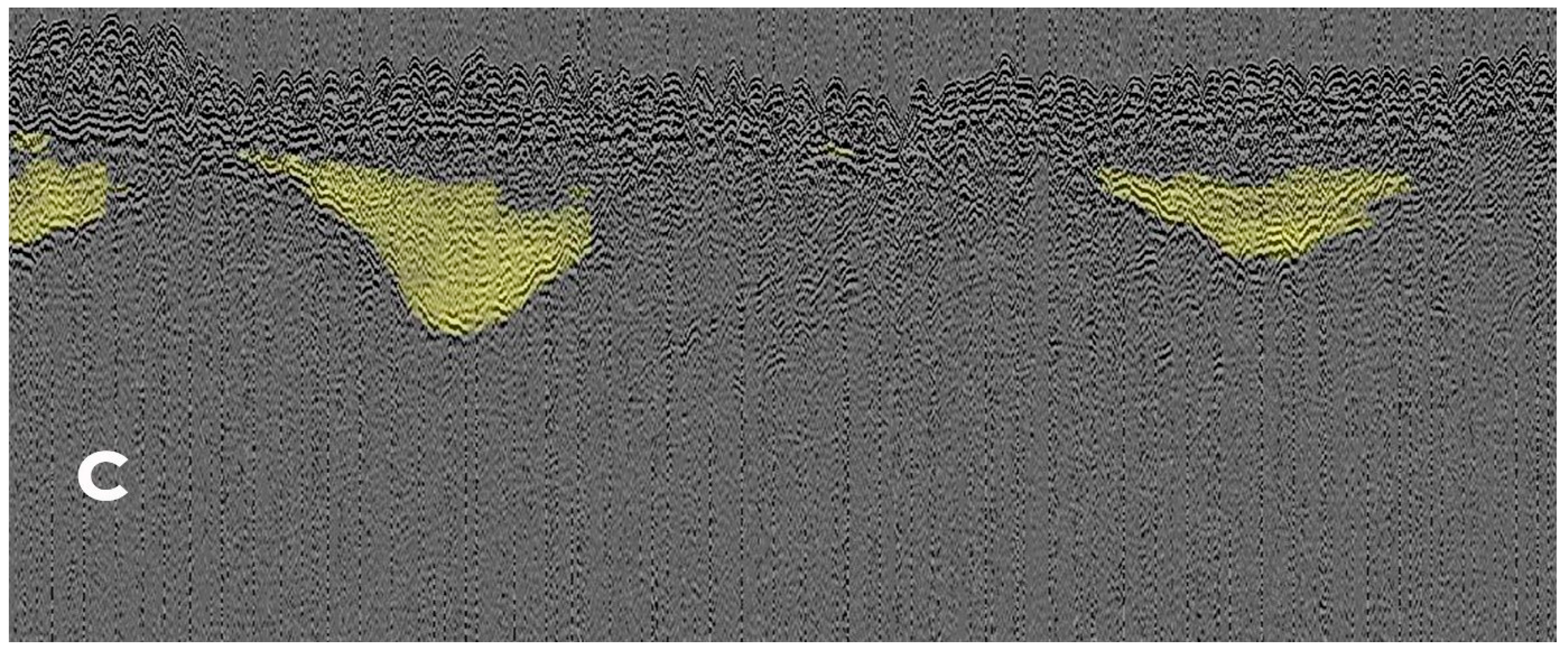
Once this had been achieved, the patches needed to be reassembled back to the original image size. To accomplish this, a mosaicking technique was used that resulted in a continuous set of 256 x 256 pixel patches. The predictions for each patch were once again merged into one image. Figures 4 A, B and C provide an example of the output: Figure 4 A shows the full-size input image in greyscale. This was split into patches for training the CNN. These AI predictions were reassembled using the mosaicking technique (Figure 4 B) and visualised as greyscale image where darker pixels represented regions of lower or zero confidence for the “feature class”, whereas brighter pixels represent predicted high confidence in the classification. To ease human interpretation this greyscale image was then filtered using the 40% threshold mentioned below and overlaid onto the original input image (Figure 4 C).
Figure 4.
A: source input image.
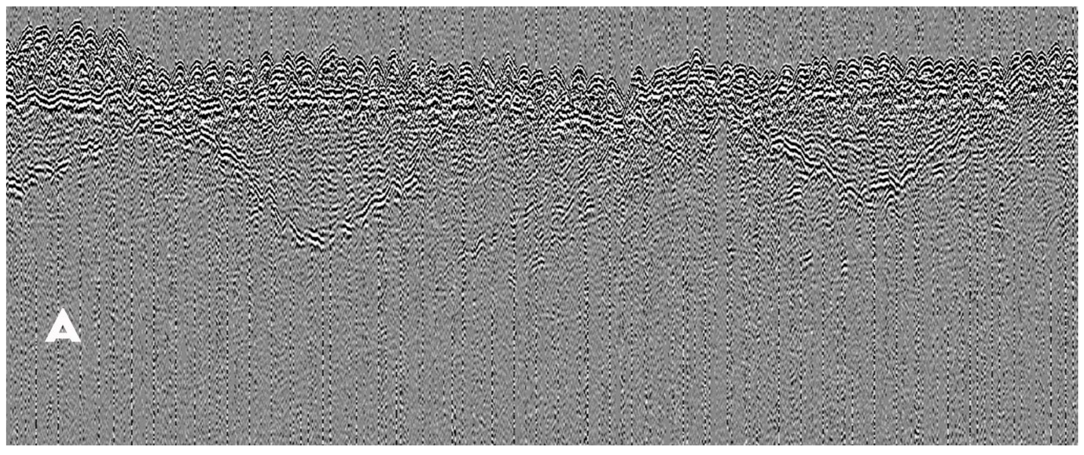
Figure 4.
B: prediction, obtained after splitting into patches, then re-assembling results.
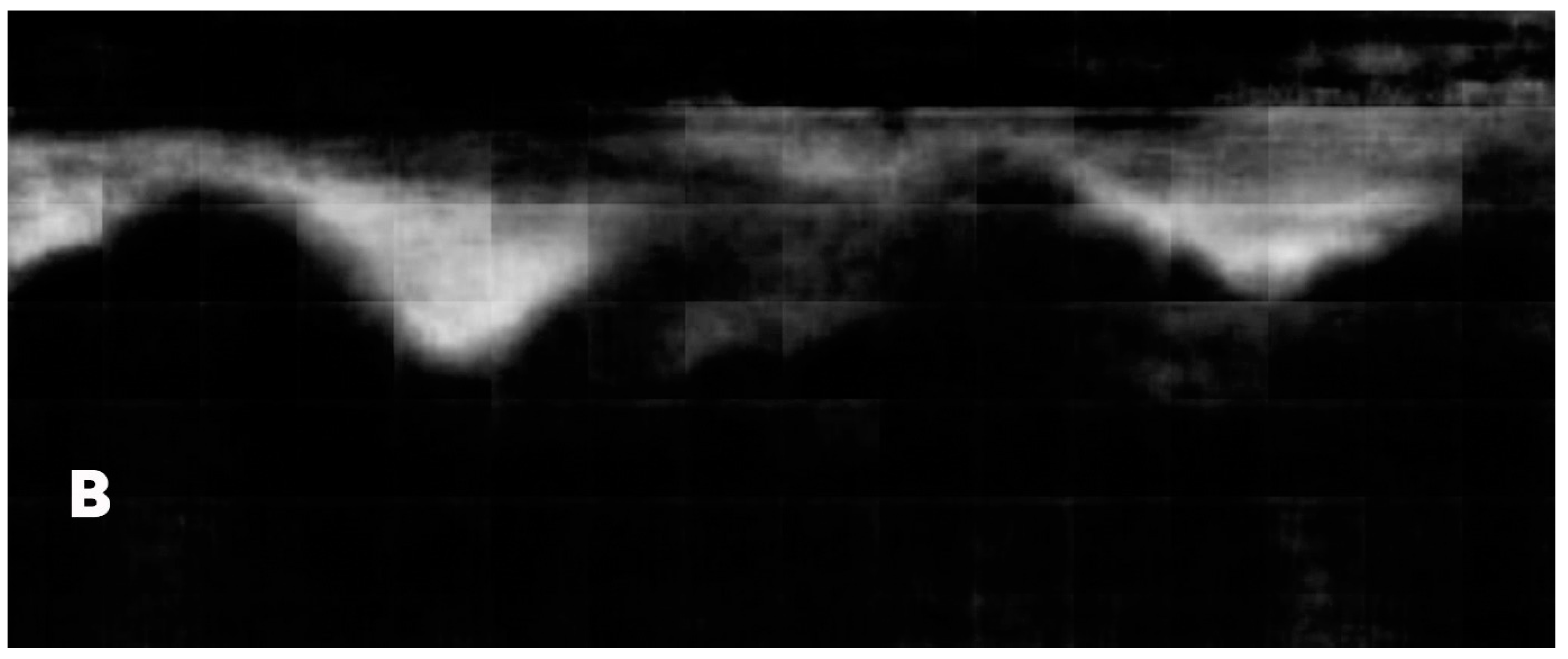
Figure 4.
C: Overlay of prediction and input.
3. Evaluation of Results
After training, a randomly selected number of images were run to test the model. Initially the results were mixed with a high occurrence of both positive and false positive classifications. To overcome this, a process, commonly referred to as Model Calibration, was employed. Confidence thresholds were changed to identify the best possible detection rate or threshold at an acceptable number of false positives. In Figure 5, correctly classified features are ringed in green, incorrectly classified (or partially classified) features in yellow and false positives are blue. Red rings denote features that were missed by the CNN. No single threshold gave perfect predictions but setting a 40% (0.4) confidence threshold returned a significantly larger proportion of positive detections to false positives. Repeated iterations of training and testing using this threshold level was found to improve the predictions still further.
When the predictive model was repeated at the 0.4 confidence threshold, the results demonstrated a suitably high level of accuracy. The model was able to reliably classify features in the sub seafloor seismic dataset, at reasonably accessible depths and containing sediment deposits.
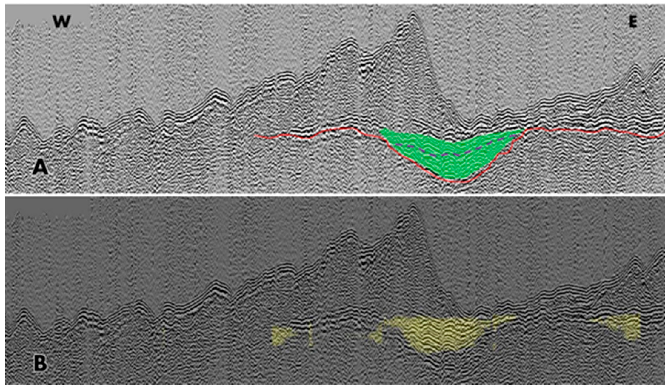
The results of running the CNN at a confidence threshold of 0.4 can be seen in Figure 6. The top set (A) is of survey line 19_1EW_pt1, shot-points 20,000-24,000, the set below (B) is of survey line BB7_WE_pt1, shot-points 64,001 – 68,000. The upper image in both A and B illustrates the simplified manually interpretation of a continuous horizon, identified as a Holocene terrestrial surface. The green fill shows the extent of a sub-seafloor topographical feature, potentially a palaeochannel, and the dashed line shows potentially important sediment deposition. The lower image in each set is the output of the CNN, run on the same seismic data but without the manual markup. The manual interpretations of these profiles were not provided to the CNN during training or the test runs.
While the CNN has not detected the full extent of the shallow features in either image, it has classified the general area and identified the continuous land surface horizon. The model has also attempted to identify possible sediment deposits within reach of a vibrocorer for sampling. The features within the second set may possibly be too deep in places, but the small feature to the left was within reach of a 6m vibrocore.
Figure 7 shows a manually interpreted seismic profile image (A) and the output of the CNN (B). Both images are from the same point of survey line Dredge2b_LF_16000-20000. Again, the CNN was run at a confidence threshold of 0.4. The merged output (B) clearly shows that the CNN was able to classify sediment deposition within the central feature at a depth that would be accessible to coring. The output also shows that the CNN correctly ignored high amplitude signals that lay outside of the feature, as well as identifying a further, small feature to the right-hand side of the image. Significantly, this feature was missed, or considered too small to be significant by the manual interpreter (A). However, the high amplitude signals suggest this as a potentially useful target.
4. Discussion & Conclusions
The output from the AI model demonstrates that focused archaeological interpretation is possible using these technologies. Although still at an early development phase, the method has proven adept at identifying features containing potential organic deposits at depths less than 6m below the sea floor, and which are accessible to sampling using a vibrocore. As a proof-of-concept model, the project demonstrates that a deep learning solution has considerable potential for exploration of seismic data for archaeological purposes.
The model achieved these results using a number of state-of-the-art AI methods to identify and classify continuous facies and sediment deposition. Predictions on positive feature identification are high (up to 88% at a threshold of 0.4) with false positives being reduced to an acceptable level. The employment of semantic segmentation demonstrated that the model can be run using images of any size as inputs.
There are, of course, improvements that could be implemented in future work. The results suggest that the AI model still performs inconsistently in accurately detecting sediments within features. A quality control method could be implemented which brings in the entire image prior to segmentation to enhance precision and validate training. There remains, however, a real need to ground truth the results in the field before future, large scale development. Manual interpretation of the seismic profiles has provided consistently high success rates in discovering peat at an accessible depth, as evidenced by the coring missions performed by VLIZ in 2018 and 2019 [7]. If the CNN can be shown to have the capacity to replicate, or even improve on, the work of manual interpretation, the outputs of AI analysis will greatly assist researchers to locate areas of high archaeological potential and ensure that coring success rates remain high.
To this end, future iterations of the CNN should focus on running the model using ‘live’ survey data as it is acquired during a marine survey. If that were achieved, this would be a true breakthrough in shallow marine geophysics. A successful application would prove immensely useful when processing the vast swathes of data now becoming available following marine development. Such automation would allow efficient processing of larger datasets, with an enhanced expectation of positive archaeological results.
Acknowledgments
The research undertaken here was supported by the award of a University of Bradford, 12-month Starter Research Fellowship to Dr Andrew Fraser. Data for the project was provided through surveys undertaken in 2018 and 2019 by the Flanders Marine Institute (VLIZ), partnered by Europe’s Lost Frontiers (supported by European Research Council funding through the European Union’s Horizon 2020 research and innovation programme – project 670518 LOST FRONTIERS, https://erc.europa.eu/ https://lostfrontiers.teamapp.com/) with additional support from the Estonian Research Council ((https://www.etag.ee; project PUTJD829). Further development of the paper was supported by the AHRC project “Taken at the Flood” (AH/W003287/1 00). The output data model, source code and training catalogue can be made available from Github on request.
References
- Münster, S.; Maiwald, F.; di Lenardo, I.; Henriksson, J.; Isaac, A.; Graf, M.M.; Beck, C.; Oomen, J. Artificial Intelligence for Digital Heritage Innovation: Setting up a R&D Agenda for Europe. Heritage 2024, 7, 794–816. [Google Scholar] [CrossRef]
- Fitch, S.; Gaffney, V.; Harding, R.; Fraser, A.; Walker, J. A Description of Palaeolandscape Features in the Southern North Sea. Chapter 3, Europe’s Lost Frontiers – Volume 1: Context and Methodologies 2022, pp 54, 59 Gaffney, V., Fitch, S., (ed.); Archaeopress 2022. [CrossRef]
- Character, L.; Ortiz Jr, A.; Beach, T.; Luzzadder-Beach, S. Archaeologic Machine Learning for Shipwreck Detection Using Lidar and Sonar. Remote Sensing 2021, 13, 1759. [Google Scholar] [CrossRef]
- Astrup, P.M.; Sea-level change in Mesolithic southern Scandinavia: long-and short-term effects on society and the environment. Chapter 2 The Mesolithic in southern Scandinavia, 2018. Jutland Archaeological Society Vol. 106 pp 20-28). Aarhus Universitetsforlag.
- Peeters, J.H.M.; Amkreutz, L.W.S.W.; Cohen, K.M.; Hijma, M.P. North Sea Prehistory Research and Management Framework (NSPRMF) 2019: retuning the research and management agenda for prehistoric landscapes and archaeology in the Dutch sector of the continental shelf; 2019. (Vol. 63). Rijksdienst voor het Cultureel Erfgoed.
- Amkreutz, L.; van der Vaart-Verschoof, S. (Eds.) Doggerland. Lost World under the North Sea; 2022. Sidestone Press, Leiden. 209 s. ISBN: 9789464261134 pp 97–106.
- Missiaen, T.; Fitch, S.; Harding, R.; Muru, M.; Fraser, A.; De Clercq, M.; Moreno, D.G.; Versteeg, W.; Busschers, F.S.; van Heteren, S.; Hijma, M.P. Targeting the Mesolithic: interdisciplinary approaches to archaeological prospection in the Brown Bank area, southern North Sea. Quaternary International 2021, 584, 141–151. [Google Scholar] [CrossRef]
- Gaffney, V.; Allaby, R.; Bates, R.; Bates, M.; Ch’ng, E.; Fitch, S.; Garwood, P.; Momber, G.; Murgatroyd, P.; Pallen, M.; Ramsey, E. Doggerland and the lost frontiers project (2015–2020). Under the sea: Archaeology and Palaeolandscapes of the Continental Shelf 2017, 305–319. [Google Scholar]
- Walker, J.; Gaffney, V.; Harding, R.; Fraser, A.; Boothby, V. Winds of Change: Urgent Challenges and Emerging Opportunities in Submerged Prehistory, a perspective from the North Sea. 2024, Heritage, Preprint, pp 10–12.
- Louwe Kooijmans, L.P.; van der Sluijs, G.K. Mesolithic bone and antler implements from the North Sea and from the Netherlands. 1971; ROB.
- Glimmerveen, J.; Mol, D.; van der Plicht, H. The Pleistocene reindeer of the North Sea—initial palaeontological data and archaeological remarks. Quaternary International 2006, 142, 242–246. [Google Scholar] [CrossRef]
- Cohen, K.M.; Westley, K.; Hijma, M.P.; Weerts, J.T.; Chapter 7: The North Sea in Flemming, N.C.; Harff, J.; Moura, D.; Burgess, A.; Bailey, G.N. (Eds.) Submerged landscapes of the European continental shelf: Quaternary paleoenvironments (Vol. 1). 2017, pp 152 - 166 John Wiley & Sons.
- Phillips, E.; Hodgson, D.M.; Emery, A.R. The Quaternary geology of the North Sea basin. Journal of Quaternary Science 2017, 32, 117–339. [Google Scholar] [CrossRef]
- Törnqvist, T.E.; Hijma, M.P. Links between early Holocene ice-sheet decay, sea-level rise and abrupt climate change. Nature Geoscience 2012, 5, 601–606. [Google Scholar] [CrossRef]
- Vashist, P. C.; Pandey, A.; Tripathi, A. A Comparative Study of Handwriting Recognition Techniques . International Conference on Computation, Automation and Knowledge Management (ICCAKM) 2020, 456–461. [Google Scholar] [CrossRef]
- Mohan, M.; Jyothi, R.L. Handwritten character recognition: a comprehensive review on geometrical analysis. IOSR J. Comput. Eng. 2015; Ver. IV.
- Bahlmann, C.; Haasdonk, B.; Burkhardt, H. Burkhardt, H.; Online handwriting recognition with support vector machines - a kernel approach, Proceedings Eighth International Workshop on Frontiers in Handwriting Recognition, 2002, pp. 49-54. [CrossRef]
- Berkson, J.M. Measurements of coherence of sound reflected from ocean sediments. The Journal of the Acoustical Society of America 1980, 68, 1436–1441. [Google Scholar] [CrossRef]
- Kreuzburg, M.; Ibenthal, M.; Janssen, M.; Rehder, G.; Voss, M.; Naumann, M.; Feldens, P. Sub-marine continuation of peat deposits from a coastal peatland in the southern baltic sea and its holocene development. Frontiers in Earth Science 2018, 6, 103. [Google Scholar] [CrossRef]
- Ball, J.E.; Anderson, D.T.; Chan, C.S. Comprehensive survey of deep learning in remote sensing: theories, tools, and challenges for the community. Journal of applied remote sensing 2017, 11, 042609–042609. [Google Scholar] [CrossRef]
- Verschoof-van der Vaart, W.B.; Landauer, J. Using CarcassonNet to automatically detect and trace hollow roads in LiDAR data from the Netherlands. Journal of Cultural Heritage 2021, 47, 143–154. [Google Scholar] [CrossRef]
- Wrona, T.; Pan, I.; Gawthorpe, R. L.; Fossen, H. Seismic facies analysis using machine learning. Geophysics Journal 2018, 83, O83–O95. [Google Scholar] [CrossRef]
- Chen, LC.; Zhu, Y.; Papandreou, G.; Schroff, F.; Adam, H. Encoder-Decoder with Atrous Separable Convolution for Semantic Image Segmentation. In: Ferrari, V., Hebert, M., Sminchisescu, C., Weiss, Y. (eds) Computer Vision ECCV 2018. Lecture Notes in Computer Science (), vol 11211. Springer, Cham. [CrossRef]
- Zhong, Z.; Zheng, L.; Kang, G.; Li, S.; Yang, Y. Random Erasing Data Augmentation. Proceedings of the AAAI Conference on Artificial Intelligence 2020, 34, 13001–13008. [Google Scholar] [CrossRef]
- Lin, T.Y.; Goyal, P.; Girshick, R.; He, K.; Dollár, P. Focal loss for dense object detection. In Proceedings of the IEEE international conference on computer vision, 2017 (pp. 2980-2988). [CrossRef]
Figure 1.
Extent of survey data acquired around the Brown Bank area of the southern North Sea. Approximate extents of coastlines are shown along with locations of prehistoric archaeological material recovered from the area (data source: SplashCOS-viewer.eu 2022).
Figure 1.
Extent of survey data acquired around the Brown Bank area of the southern North Sea. Approximate extents of coastlines are shown along with locations of prehistoric archaeological material recovered from the area (data source: SplashCOS-viewer.eu 2022).
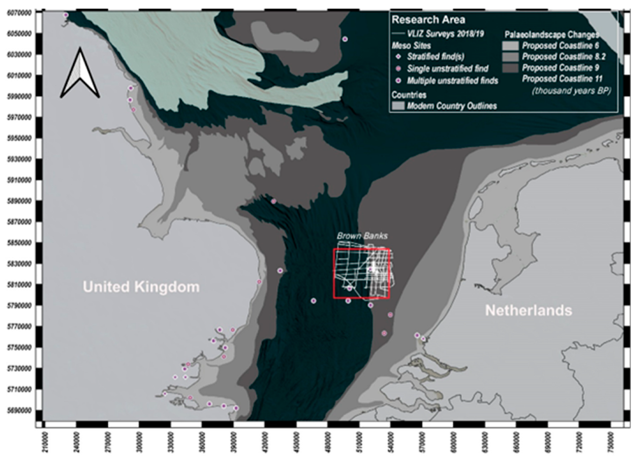
Figure 2.
Training data comprised of simplified interpretations over a seismic profile, here showing a marked horizon and landscape feature (green). It also shows significant sediment deposition (red dashed line). Each image used comprised 4,000 traces at a resolution of 1600 x 600px.
Figure 2.
Training data comprised of simplified interpretations over a seismic profile, here showing a marked horizon and landscape feature (green). It also shows significant sediment deposition (red dashed line). Each image used comprised 4,000 traces at a resolution of 1600 x 600px.
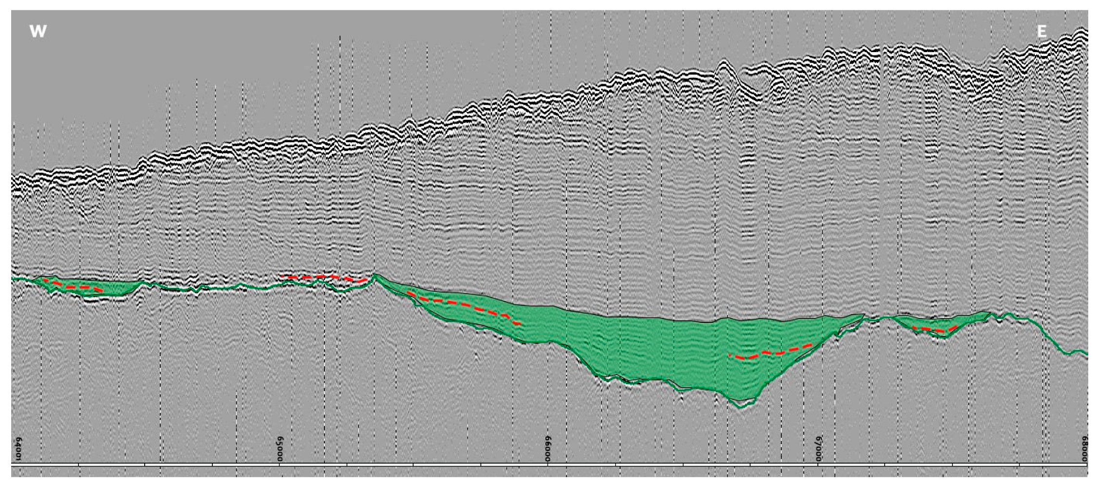
Figure 3.
Demonstration of the improved loss through 35 epochs of the deep learning model. Each CNN was trained over up to 35 epochs. (X axis shows batches, Y axis is loss, data in blue is training loss, orange is validation loss).
Figure 3.
Demonstration of the improved loss through 35 epochs of the deep learning model. Each CNN was trained over up to 35 epochs. (X axis shows batches, Y axis is loss, data in blue is training loss, orange is validation loss).
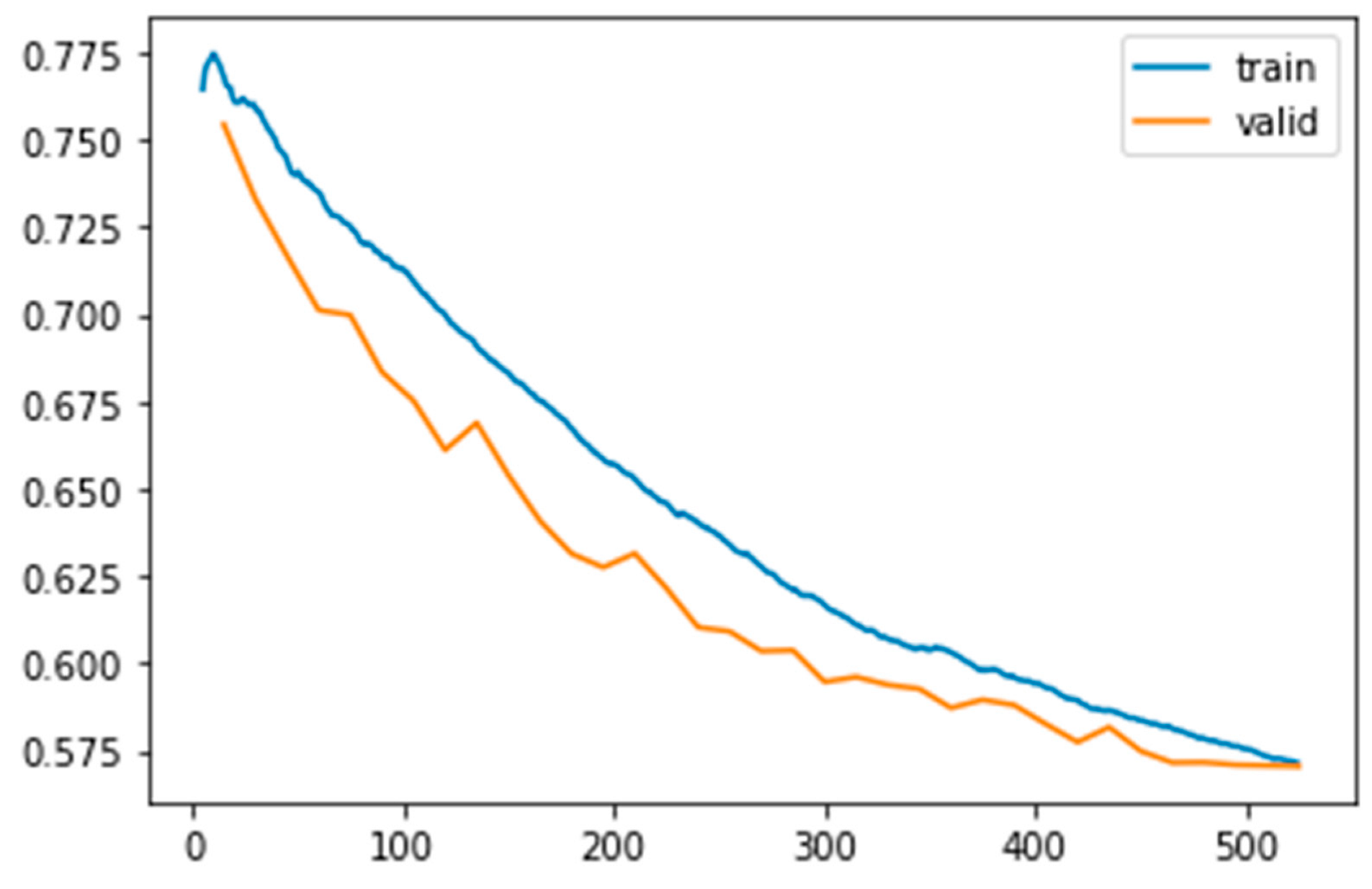
Figure 5.
Predictive classification results using different confidence thresholds (0.3-0.6). Correctly classified (green), incorrectly or partially classified in yellow, false positives (blue) and features missed by the CNN (red).
Figure 5.
Predictive classification results using different confidence thresholds (0.3-0.6). Correctly classified (green), incorrectly or partially classified in yellow, false positives (blue) and features missed by the CNN (red).
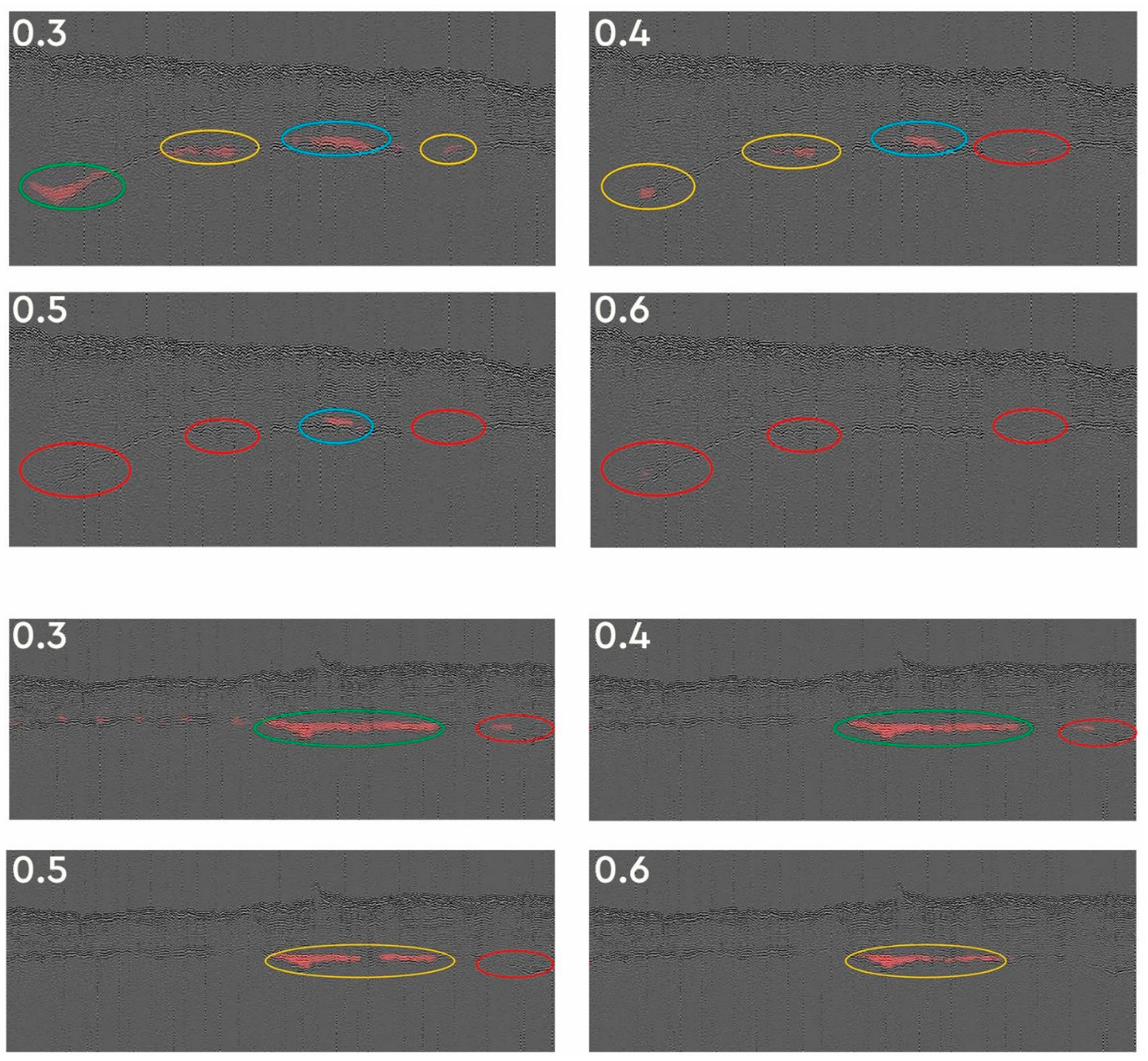
Figure 6.
two sets of images (A & B) showing a feature with depositional fill. Each set comprises a simplified manual interpretation (A1 & B1) and the AI test results for the same image minus the interpretation (A2 & B2). AI colours represent different runs using the same CNN.
Figure 6.
two sets of images (A & B) showing a feature with depositional fill. Each set comprises a simplified manual interpretation (A1 & B1) and the AI test results for the same image minus the interpretation (A2 & B2). AI colours represent different runs using the same CNN.
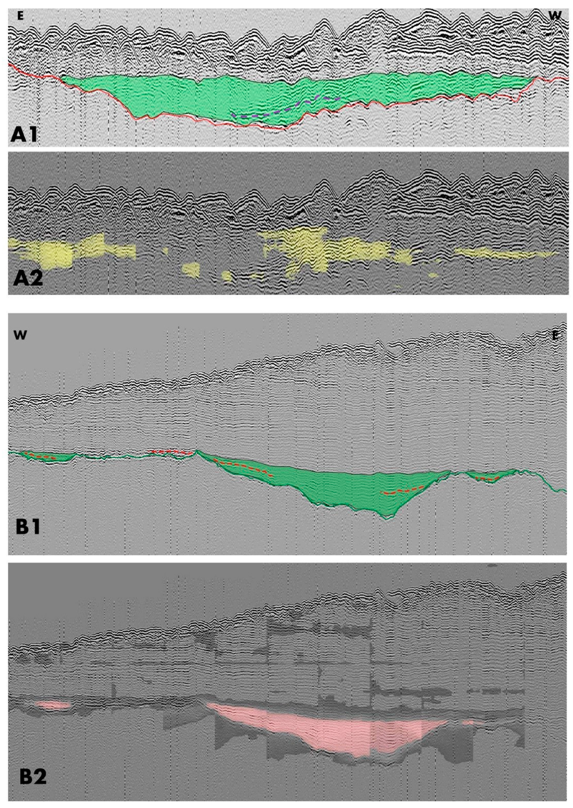
Figure 7.
Two images of the same seismic profile (A & B). The upper shows a simplified manual interpretation, the lower shows the AI interpretation.
Figure 7.
Two images of the same seismic profile (A & B). The upper shows a simplified manual interpretation, the lower shows the AI interpretation.
Disclaimer/Publisher’s Note: The statements, opinions and data contained in all publications are solely those of the individual author(s) and contributor(s) and not of MDPI and/or the editor(s). MDPI and/or the editor(s) disclaim responsibility for any injury to people or property resulting from any ideas, methods, instructions or products referred to in the content. |
© 2024 by the authors. Licensee MDPI, Basel, Switzerland. This article is an open access article distributed under the terms and conditions of the Creative Commons Attribution (CC BY) license (https://creativecommons.org/licenses/by/4.0/).
Copyright: This open access article is published under a Creative Commons CC BY 4.0 license, which permit the free download, distribution, and reuse, provided that the author and preprint are cited in any reuse.


