Submitted:
26 February 2024
Posted:
27 February 2024
You are already at the latest version
Abstract
This paper analyses the application of deep learning techniques for predicting wave overtopping events in port environments using sea state and weather forecasts as inputs. The study was conducted in the outer port of Punta Langosteira, A Coruña, Spain. A video recording infrastructure was installed to monitor overtopping events from 2015 to 2022, identifying 3709 overtopping events. The data collected was merged with actual and predicted data for the sea state and weather conditions during the overtopping events, creating three datasets. We used these datasets to create several machine learning models to predict whether an overtopping event would occur based on sea state and weather conditions. The final models achieved a high accuracy level during the training and testing stages: 0.81, 0.73, and 0.84 average accuracy during training and 0.67, 0.48, and 0.86 average accuracy during testing, respectively. The results of this study have significant implications for port safety and efficiency, as wave overtopping events can cause disruptions and potential damage. Using deep learning techniques for overtopping prediction can help port managers take preventative measures and optimize operations, ultimately improving safety and helping to minimize the economic impact that overtopping events have on the port's activities.
Keywords:
machine learning
; neural networks
; deep learning
; wave overtopping prediction
; port management
; port security
1. Introduction
Around 80% of the goods we consume are carried by ships due to shipping’s ability to offer economical and efficient long-distance transport. These goods include raw materials that need to be processed and products like food, medical supplies, fuel, clothes, and other essential goods ready to be consumed [1].
Maritime trade has increased almost yearly since 1970, except for 2020, due to the global COVID-19 pandemic [1]. We can also observe this growing trend in maritime trade in Europe, where many countries have invested in maritime port infrastructures [2], including Spain, where this work took place [3].
The existence of a worldwide transport network and the globalization of production and consumption have fostered competition between ports to attract the largest number of customers. In order to attract more customers, port terminals must be as competitive as possible [4]. A port must be safe and efficient to be competitive. These two characteristics are not mutually exclusive, and measures to improve safety would also impact efficiency and vice versa.
Besides having good shelter conditions, connections, and large surfaces for product handling and storage, the ship’s stay in port must be safe, allowing it to carry out loading and unloading operations securely. Safety also includes the physical safeguard of port personnel working on port operations (besides loading and unloading cargo).
The overall importance of maritime trade in the world economies due to its weight in the consumption economies, and the particular importance in the case of Spain, reveals that events that could disrupt the normal operations of a port, impacting the operation safety or performance, can have a significant negative economic impact. This importance also reveals that improvements in safety or optimizations of operations in a port can have a significant positive economic impact.
A commercial port aims to harbour ships and provide safe loading areas where ships can load and unload cargo (or passengers). A loading area is only safe if the port has some large structure that shelters and protects the moored ships there from the force of powerful waves.
One element a port uses to protect the loading areas is a breakwater (also known as a jetty). A breakwater is a permanent protective structure built in a coastal area to protect anchorages against waves, tides, currents, and storm surges. A breakwater achieves this protection through the reflection and dissipation of the incident wave energy. Although breakwaters may also be used to reduce coastal erosion, for instance, to protect beaches, this work focused on studying breakwaters as a port protection structure.
A breakwater may be connected to land or freestanding and may contain a walkway or road for vehicle access. A standard breakwater section is usually composed of a core made of granular material, protected with armour layers of rockfill (or riprap, or different pieces like cubes, tetrapod and similar elements), and covered with a superstructure of mass or reinforced concrete.
The most conventional types of breakwaters are vertical, composite, and sloping (or rubble-mound). We can see these three types of breakwaters in Figure 1a (source [5]), where h is the depth at the site, and H, L, FC, and B are, respectively, the characteristic wave height, characteristic wavelength, freeboard, and the representative magnitude of the breakwater width.
Figure 1b (source [6]) shows a sloping breakwater with all the previously explained elements. This image corresponds to the outer port of A Coruña, Spain, where we carried out the primary fieldwork of this work.
Even a properly designed breakwater cannot protect the ships anchored there from all the possible wave-caused phenomena. I.e. a breakwater protects up to a point; it is designed to protect against phenomena up to a given magnitude. However, budget and physical constraints do not allow building a breakwater to protect ships against every wave-caused phenomenon.
The main disrupting wave-related event that could hinder the protection offered by a breakwater is wave overtopping. Wave overtopping is a dangerous phenomenon that occurs when waves meet a submerged reef or structure or an emerged reef or structure with a height up to double the approximate wave height. The latter case is the one that affects a port’s breakwater and the one studied in this work.
During an overtopping, two processes occur: wave transmission and water passing over the structure. This work focuses on measuring the passing of water over the structure (a breakwater in this case). This process can occur in three different ways, either independently of each other or combined:
- Green Water is the solid (continuous) step of a given volume of water above the breakwater’s crown wall due to the wave’s rise (wave run-up) above the exposed surface of the said breakwater.
- White Water occurs when the wave breaks against the seaside slope. This event creates so much turbulence that air is entrained into the water body, forming a bubbly or aerated and unstable current and water springs that reach the protected area of the structure either by the wave’s impulse or as a result of the wind.
- Aerosol is generated by the wind passing by the crest of the waves near the breakwater. Aerosol is not an especially meaningful event in terms of the damage it can produce, even in the case of storms. This case is the least dangerous of the three, and its impact on the normal development of port activities is negligible.
Regarding the damage they could cause, the more critical overtopping types are green and white water. So, this work focused on these overtopping types. Figure 2 shows an example of white water overtopping captured on the outer port of Punta Langosteira, A Coruña, as part of this work.
1.1. Recommendations for overtopping limits and mitigation
A breakwater constructed to protect a harbour area should satisfy rigorous conditions if we want to reduce wave overtopping and its impact. Several proposals in the literature define those conditions and propose recommendations to study wave overtopping. The most widely used manual regarding wave overtopping is the EurOtop manual [7], which guides designers and operators of breakwaters, reclamations, inland lakes or reservoirs on analysing and predicting wave overtopping for flood defences attacked by wave action. The manual describes the main variables involved in an overtopping event and provides formulas and tools for predicting said events based on tests carried out in hydraulic laboratories. However, the manual notes that one must consider the specific characteristics of a port when using these resources due to the sensitivity of overtopping to changes in the geometry of the port, incident waves, and the local bathymetry.
Although it is impossible to establish precise limits to tolerable overtopping for all conditions, this manual includes some guidance on tolerable mean discharges and maximum overtopping volumes for various circumstances or uses. The manual also emphasises that these limits may be adopted or modified depending on the site’s circumstances and uses.
Another recommendation for the conditions a breakwater should satisfy to protect a harbour area by reducing wave overtopping and its impact is the Spanish Ports System’s Recommendations for Breakwater Construction Projects, ROM 1.1-18 [5]. ROM 1.1-18, for instance, indicates that the conditions a breakwater satisfies regarding wave energy transmission, either from the overtopping of the crown or propagation through the breakwater section, are the following: the breakwater’s relative height (h + FC)/H, generally has dimensions on the order of 1, O(1), and relative width, B/L, on the order of 1/10, O(1/10), where h is the depth at the site; and H, L, FC, B are, respectively, the characteristic wave height, characteristic wavelength, freeboard, and the representative magnitude of the breakwater width (see Figure 1).
When a wave overtopping occurs in a commercial port environment, the best-case scenario will be the disruption of activities. Even this scenario has negative financial repercussions. A system that detects overtopping events would provide valuable information to port operators, allowing the minimisation of the impact of overtopping: the financial impact, the property damage, or even physical harm to port workers. Wave overtopping has traditionally been studied from three possible approaches: small-scale physical modelling, numerical modelling, and in situ measurement.
1.2. Overtopping: small-scale physical modelling
Small-scale physical modelling has traditionally been one of the most used techniques for studying wave overtopping. It involves a small-scale port model, where the overtopping will be studied. These models allow the reproduction of the most significant physical phenomena that intervene in overtopping.
In this type of modelling, the tests are usually conducted using a wave energy spectrum, which is then used to generate a free surface wave time series at the wave paddle. When the water overpasses the model’s breakwater due to overtopping, it is channelled and collected using structures built to measure the overtopping water volume.
Small-scale modelling is used, for instance, to determine the influence of certain factors in wave overtopping. For example, in [8], the authors studied the influence of wind waves on overtopping.
The methods involved in this type of modelling continue to evolve. The tests usually use a wave energy spectrum free surface wave time series at the wave paddle. Although this method could generate an infinite number of time series, only one is usually generated due to the expense of running multiple tests in a physical model. Hannah et al. proposed an improvement of this method in [9], where the authors used several time series generated from the same wave energy spectrum to study the variation in the main overtopping measures. As a result, they show that using different time series gives different results for some of the overtopping measures, indicating that this is the correct approach.
This method continues to generate new knowledge. For instance, Lashley et al. [10] proposed a new formula for calculating wave overtopping at vertical and sloping structures with shallow foreshores using deep-water wave characteristics. Another example is the work of Orimoloye et al. [11], where the authors conducted an experimental study focusing on overtopping characteristics of coastal seawalls under random bimodal waves and, based on the experimental results, proposed a modification to the EurOtop formula to capture the overtopping discharge under bimodal conditions better.
An example of a different technique for detecting overtopping events is the one used by Formentin and Zanuttigh [12]. In this work, the authors used a semi-automatic and customisable method based on a threshold-down-crossing analysis of the sea surface elevation signals obtained using consecutive gauges. They applied their method to new and past data and compared the results with well-established formulae, obtaining accurate and reliable results.
Although new and clever techniques exist to measure overtopping on a physical model, the downside is that some are effective in a laboratory but not practical in a real environment due to the high amount of elements required or the need to construct a gigantic structure to collect the water of an overtopping event, and the high economic cost and time consumption.
1.3. Overtopping: numerical modelling
The development of computational models for overtopping simulations progressed along with the advances in computing power. For example, some works analyse the wave-infrastructure interaction using 2D or 3D models to study overtopping [13,14,15]. Alternatively, other works use Machine Learning models to do water flow estimations during overtopping [16] or predict overtopping events [17,18].
Public institutions and private companies have developed software which includes computational models for overtopping simulations. An example of such a tool is the widely used Computational Fluid Dynamics Toolbox OpenFoam [19]. OpenFOAM has many features to solve complex fluid flows involving chemical reactions, turbulence and heat transfer, acoustics, solid mechanics and electromagnetics.
Although not technically numerical modelling, it is worth mentioning that with the first EurOtop manual in 2007, they also developed an online Calculation Tool to assist the user through a series of steps to establish overtopping predictions for embankments and dikes, rubble mound structures, and vertical structures. Due to lacking funds, they could not update the web-based Calculation Tool with the new formulae in the manual’s latest edition. They removed the old calculation tool from the website but kept PC-Overtopping, a PC version of the tool [20].
Also, in parallel with the EurOtop manual, the authors developed an Artificial Neural Network called the EurOtop ANN. This ANN can predict the mean overtopping discharge using the hydraulic and geometrical parameters of the structure as inputs. The authors created this ANN using the extensive EurOtop database extended from the CLASH database, which contains more than 13,000 tests on wave overtopping. The ANN and both databases are free and available through links on the website [21,22].
Although the evolution and support experienced by tools like OpenFOAM and the EurOtop tools have positioned them as a viable alternative to physical modelling due to their low cost and adaptability, they present the same limitation of physical modelling. These limitations are caused by adopting simplifications of reality in the model to maintain an acceptable computational cost. Another problem with these numerical models is that, given the phenomena’ complexity, real data should be used to validate the models whenever possible.
1.4. Overtopping: in situ measuring
The third alternative for analysing the wave overtopping phenomenon is in situ measurement, i.e., using devices that record or measure overtopping events in a real scenario.
An example of in situ measuring of wave overtopping is the work of Briganti et al. [23]. In this work, the authors measured wave overtopping at the rubble mound breakwater of the Rome–Ostia yacht harbour, constructing a full-scale station similar to the ones used in small-scale physical modelling. This structure collects the water of an overtopping event and allows measuring it. The authors studied wave overtopping during one measurement campaign (2003-2004) and compared the data to the predictions obtained using known formulae based on small-scale model tests. Their results show that these formulae tend to underestimate overtopping events. The same port was also studied in a later work [24]. A similar method was used to study the Zeebrugge port in Belgium [25].
Modern approaches to detecting wave overtopping involve using image devices. For instance, Ishimoto Chiba and Kajiya [26] created a system that used video cameras to detect an overtopping event. The authors set trigger points in different areas of the video cameras’ images, and the system could detect overtopping in those areas. When an overtopping was detected, the system sent several images (pre and post-overtopping) to the servers, where they were analysed.
Similar work was done by Seki, Taniguchi, and Hashimoto [27], where the authors created a method for detecting the overtopping wave and other high waves using images from video cameras. In this work, the authors detected overtopping by measuring the wave contour in every video frame using Active Contour Models and tracking the contour. This method has the advantage of being robust to other moving objects. The authors showed the effectiveness of their method by experimenting with actual video sequences of both a typhoon approaching and calm scenes.
More recently, Chi et al. [28] used a shore-based video monitoring system to collect coastal images of wave overtopping at a 360m long sea dike during a storm in July 2018 at Rizhao Coast, China. The system captured images with a sampling frequency of 1 Hz in the beginning 10 min of each hour during daylight. Using the images, the authors calculated the frequency, location, width and duration of individual overtopping events, detecting 6,252 individual overtopping events during the ten-hour storm. The results of this work indicate the feasibility of a shore-based video monitoring approach to capture the main features of wave overtopping in a safe and labour-saving manner while enabling a detailed analysis of the temporal and spatial variation of wave overtopping.
Despite providing precious information for detecting the problems that affect a given installation, in situ measurement constitutes a less widespread methodology than physical or numerical modelling. This less general usage of in situ measuring is mainly due to the high economic cost involved, on the one hand, in acquiring monitoring equipment and, on the other, in carrying out extensive field campaigns. Despite the smaller number of scientific studies using in situ measuring and the low amount of data they collect compared to the other techniques, in situ measuring is a good tool for evaluating operational problems in port facilities due to overtopping events.
Wave overtopping events have an enormous negative impact on a port in terms of the safety of workers and the efficiency of operations. Due to climate change, sea levels are expected to rise, and the frequency and magnitude of overtopping events are expected to increase. Current estimations project that by the end of the 21st century, the globally aggregated annual overtopping hours will be up to 50 times larger than in the present day [29]. This current and future dangerous situation increases the relevance of detecting and quantifying the wave overtopping phenomenon. The best way to do so is to facilitate in situ measuring overtopping events by developing easy-to-use techniques that use low-cost measuring equipment while providing good results.
2. Materials and Methods
The wave overtopping events data was collected in six field campaigns in the outer port of Punta Langosteira (A Coruña) from 2015 until 2020. During these campaigns, 3098 individual overtopping events were identified. The overtopping events data was integrated with the environmental data (weather conditions and sea state) the port was subject to during the overtopping events to assemble the datasets used to create several Machine Learning overtopping prediction models.
The overtopping prediction is a classification problem: a model predicts a positive event (overtopping) if the model output exceeds the decision threshold and a negative one (no overtopping) if not.
Besides creating the models, the decision threshold must be studied to evaluate how its value impacts the tradeoff between security and economic cost: a low decision threshold would capture many overtopping events, providing more security, but would have many false positives incurring in higher costs due to stopping port operations; having a higher decision threshold would capture less overtopping events but with more certainty (less false positives), providing less security, but incurring in lower operational costs due to stopping port operations only with a higher certainty of an overtopping event.
In a classification problem, the model’s accuracy is usually used as the metric to evaluate its performance, but this is not the best approach if the data is not balanced (when there are several times more samples from one target class (majority class) than from the other (minority class)).
There are several more appropriate metrics (than the accuracy) when dealing with unbalanced datasets that mainly rely on precision and recall, such as the F1 score (the harmonic mean of the precision and recall) or the more general F-measure is the weighted harmonic mean of the precision and recall.
No consensus exists on which prevalence values make a dataset imbalanced. In this work, we consider the ranges defined in [30] that indicate the degree of imbalance of a dataset given the percentage of examples belonging to the minority class on the dataset: 20-40% mild, 1-20% moderate, and <1% extreme imbalance.
In order to study how a classifier will behave when changing the decision threshold, more advanced metrics, such as the ROC curve and the associated AUROC [31,32], can be used. However, these metrics are inappropriate when working with imbalanced datasets [33]. In this case, it is better to use the precision-recall curve, which computes a curve from the raw classifier output by varying the decision threshold and calculating the precision and recall at every threshold value. The area under the precision-recall curve can be estimated using the average precision (AP, with values between 0 and 1; the higher, the better). There are multiple ways of calculating the AP. This work uses the definition:
where Pn and Rn are the precision and recall at the nth threshold. Calculating the area under the curve does not use linear interpolation of points on the precision-recall curve because it provides an overly optimistic measure of the classifier performance [34,35].
Another essential aspect when dealing with an imbalanced dataset is appropriately separating the data into folds when using k-fold cross-validation to choose among several models (validation). Using regular k-fold in imbalanced datasets could cause many folds to have just examples of the majority class, negatively affecting the training process. In such cases, it is recommended to use stratified sampling (stratified k-fold) to ensure that the relative class frequencies are (approximately) preserved in each train and validation fold.
The variables used to create the wave overtopping prediction models can be classified into meteorological conditions (weather conditions and sea state) and overtopping characteristics (location, number of events, and size). The models use the meteorological conditions as inputs and a binary output that indicates whether an overtopping event will happen.
Three dataset variants were created in order to assess which one works better. Two use real historical data for the sea state and weather conditions. The third uses the historical data of the Portus forecasting system (the stored predictions instead of real data).
The real data presents more variation than the predictions, and the model could, a priori, better capture the relationship between the actual sea state and weather conditions and the overtopping events.
The historical data of the forecasting system was used for the third dataset variant because the production system will use the forecast data as input to the models. Thus, training the models on data belonging to the same distribution of the production data could provide better results.
For the datasets based on real historical data, the weather conditions and sea state data were gathered using the three measurement systems provided by the port technological infrastructure: a directional wave buoy, a weather station and a tide gauge.
The directional wave buoy is located 1.8 km off the main breakwater of the port (43º21′00′′ N 8º33′36′′ W). This buoy belongs to the Coastal Buoy Network of Puertos del Estado (REDCOS [36]) and has the code 1239 in said network. Due to the sensibility of the buoy data to noise, the system provides its data aggregated in 1 h intervals. This quantization allows the calculation of some statistical parameters that reflect the sea state while mitigating the noise’s effects.
The weather station is located on the main port’s breakwater. It belongs to the Port Meteorological Stations Network (REMPOR [37]) and provides data aggregated in 10-minute intervals.
The tide gauge is also placed at the end of the main port’s breakwater and belongs to the Coastal Tide Gauges Network of Puertos del Estado (REDMAR [38]), with code 3214 on said network. It provides the data in 1-minute intervals.
From all the variables these data sources provide, only the ones that were also available in the port’s forecast system were chosen to create the first dataset. This work aims to create wave overtopping prediction models that can predict an overtopping event using weather and sea state forecasts as inputs. In order to fulfil this objective, the models’ inputs regarding ocean-meteorological variables must be available in the port’s forecast system.
The second dataset adds the maximum wave height variable to the previous one. This variable is currently unavailable as forecast, but Portus is currently modifying its forecasting models to include it, so this dataset was created to assess whether the inclusion of this variable will provide better results once this information is available.
These are all the meteorological variables available to use as input variables to the models:
- HS (m): the significant wave height, i.e., the mean of the highest third of the waves in a time series representing a specific sea state.
- Hmax (m): the maximum wave height, i.e., the height of the highest wave in a time series representing a specific sea state. This variable is used only in the second dataset and is not available as forecast.
- TP (s): the peak wave period, i.e., the period of the waves with the highest energy, extracted from the spectral analysis of the wave energy.
- θm (deg): the mean wave direction, i.e., the mean of all the individual wave directions in a time series representing a specific sea state.
- WS (km/h): the mean wind speed.
- Wd (deg): the mean wind direction.
- H0 (m): the sea level with respect to the zero of the port.
- H0 state: a calculated variable created to indicate whether the tide is rising, high or low, or falling (1, 0, -1).
- H0 min (m): the minimum sea level with respect to the zero of the port achieved during the current tide.
- H0 max (m): the maximum sea level with respect to the zero of the port achieved during the current tide.
In the datasets based on real historical data for the sea state and weather conditions, the buoy provides HS, TP and θm, the weather station provides Ws and Wd, and the tide gauge provides H0 and Hmax. The rest of the variables are calculated from the raw data.
The Portus system provides all the data for the dataset based on historical forecasted data.
The three datasets use whether an overtopping event occurred or not as the model’s output.
During the field campaigns for collecting overtopping data, the buoy and tide gauge in the outer port malfunctioned several times due to storms and other phenomena. Due to this, there are many overtopping events for which there are no associated real meteorological and sea state conditions, only the historical predicted data. Hence, the dataset based on predicted conditions has more examples than the ones based on real conditions (as shown in Table 1).
Creating the datasets based on real data involved joining the data provided by the available data sources (buoy, weather station, and tide gauge). These data sources use different data sampling frequencies, so all the data had to be aggregated to have the same frequency as the frequency of the data with the largest period, the sea state data. This data has a period of 1 hour, the same as the forecast systems predictions (the data that will be used as the models’ inputs in production).
The overtopping events had to be aggregated accordingly. For this, the number of events and their magnitudes were aggregated for every hour, and the output label was set to one if one or more overtopping events happened during the hour and zero otherwise.
After merging, the data was preprocessed to improve the models’ performance. Since θm and Wd are directional variables in the 0-360 degrees range, 0 and 360 represent the same direction. Using this codification for the directional variables would cause the Machine Learning models to create different internal representations for the same state and could negatively impact the models’ performance. This potential problem was avoided using the sine and cosine for each value, so the 0 and 360 directions are close together (sin and cosine vary continuously from 0 to 360).
In the final datasets, the positive examples of overtopping events represent around 1.2% of the total on the two real data datasets and around 1.5% on the dataset based on predictions. These figures situate these datasets on the lower bound for moderate imbalance datasets, making them almost extremely imbalanced. Due to this, we used the appropriate metrics that consider the data imbalance, as previously explained.
Once merged, aggregated, and preprocessed, the data sources were separated into the corresponding training and testing datasets, used to train and test the different models. The test dataset is usually created by randomly choosing data from the whole dataset. However, having imbalanced datasets would cause the test results to be inaccurate, and the models could be trained with just negative examples, potentially giving the models excellent and unrealistic training results. To avoid these problems, the test sets were created so that they contain a proportion of positive overtopping instances similar to the corresponding training dataset: in each dataset, the testing dataset is around 1/3 of the whole dataset, and the proportions of positive and negative examples are similar among the training and testing datasets, as shown in Table 1.
Hundreds of models based on artificial neural networks were created, trained with the three datasets previously explained, and compared to check which model and dataset combination provided the best results.
The models are based on artificial neural networks (ANNs) [39], given the good results this machine learning model can achieve for classification problems. Given that this models require choosing multiple hyperparameters (number of layers, nodes per layer, and training parameters, among others explained later), we used an iterative approach to choose the best hyperparameters while reducing the time required to obtain them:
- First, several allowed values for each hyperparameter are manually specified, and a hyperparameter grid is created (the outer product of all hyperparameters’ values, i.e., all possible combinations).
- Then, as many individual models as combinations in the grid are created, trained, and compared using cross-validation.
- The results are analysed, focusing on the grid regions where the best results were obtained to create a new grid to contain that region.
- Steps 2-3 are repeated several times for each dataset until a satisfactory cross-validation performance is obtained.
The hyperparameters and all the values tested with this approach are the following:
- Network architecture: We tested networks with 1, 2, 3 and 4 layers. Also tested were 8, 16, 32, 64, 128, and 256 neurons per layer in each case, allowing each layer to use a different number of neurons. All ANNS used fully connected layers. Although the largest networks could seem too complex for the overtopping prediction problem, they were included to use dropout regularisation. Dropout will likely get better performance on a larger network (it will prune the network, resulting in a smaller one).
- Optimiser: The Adam [42] optimiser was used.
- Training iterations: The optimiser was tested with 500, 1,000, 1,500, 2,000, and 5,000 iterations. In the initial tests, the results did not improve from 2,500 iterations up, so the 5,000 values were discarded for the subsequent iterations of the hyperparameters search approach.
- Activation function: All the ANNs used the ReLU activation function for the neurons in the hidden layers and the sigmoid function for the output layer.
- Regularisation: The ANNS were regularised using dropout regularisation [43], with one dropout layer for each hidden layer (except the output layer). Several dropout rates were tested: None, 0.0625, 0.125, 0.25, 0.375, and 0.25, where None indicates that no dropout was used.
- Layer weight constraints: A maximum norm constraint on the model parameters was set during training to avoid overfitting. I.e. constraints were put on the weights incident to each hidden unit to have a norm less than or equal to the desired value. The values None, 1, 3, and 5 were tested, where None indicates no constraint.
- Learning rate (lr): The values 0.00001, 0.0001, 0.001, and 0.01 were tested for the learning rate. Although 0.01 is usually considered too large a learning rate, large values are suggested in the original dropout paper [43].
- Batch size: The datasets have several thousand examples, so several batch size values were tested to speed up the training process (the dataset is divided into smaller batches, and the network weights will be updated after processing each batch). The None, 100, 500, and 1000 values were tested, where None indicates that the whole dataset is to be processed before updating the model’s parameters (weights).
As previously explained, the wave overtopping dataset is a moderate-extreme imbalanced dataset. In an imbalanced dataset, regular k-fold cross-validation could potentially give incorrect results [44]. This potential problem was avoided using stratified k-fold, so all the folds used during cross-validation have similar class proportions.
In this problem, we are most interested in obtaining a model that detects as many overtopping events as possible (high recall) to increase the port’s safety while having low false positives (high precision) to maximize the port’s operativity. Precision and recall are increased and decreased by varying the decision boundary of the ANN’s raw output sigmoid function, but usually, increasing one decreases the other. The port’s stakeholders are still determining which decision boundary (threshold) is the one that gives the best tradeoff from a practical perspective of the port’s safety and performance. Some metrics, such as the balanced accuracy and the F-score, use a 0.5 decision threshold. We used the average precision to choose the best model in cross-validation (although we calculated several metrics to see the models’ performance). As previously explained, the average precision calculates the model’s overall performance when varying this threshold by obtaining the precision and recall for each threshold and calculating the area under the curve this creates.
Once we trained all the models using cross-validation and the iterative process previously explained, the best model for each dataset was selected and retrained on the whole train dataset (each model in its corresponding dataset). Once the final best three models were obtained, their performance was evaluated using the corresponding testing datasets. The whole process of creating the ANNs overtopping prediction models is summarised in Table 2.
3. Results
As explained earlier, several cross-validation metrics were calculated to visualise how the models behave during training (using cross-validation), although the deciding metric was the average precision. Thus, each model’s precision, recall, f1 score, and average precision were calculated.
Table 3 shows the hyperparameters for the best ANN model obtained using the previously described training method. The table shows the best model for each metric used, allowing us to analyse the impact of each metric during cross-validation, i.e., which model would have been chosen had we used the corresponding metric. However, the deciding metric is the average precision for the reasons previously explained.
In this table and all the following tables and figures, models 1 and 2 are the ones trained on historical real data, model 2 being the one that includes the hmax variable, and model 3 is the one trained on historical predicted data.
Table 3 shows that model 3 obtained the best results during validation, with an average precision of 0.82. Models 1 and 2 performed similarly, with an AP of 0.81. A fairly large Neural Network, with three hidden layers, is needed to solve the problem, resulting in a network of five layers (hidden plus input and output layers). The highest precision, 1, is achieved by a model trained on dataset 3, but the higher recall, 0.81, is obtained by a model trained on dataset 1.
After training the best model (the one with the best AP during validation), the three models’ performance in the training dataset for different thresholds was compared using their PR curves, as shown in Figure 3.
Figure 3 shows that model 3 obtained the best results, with an AP of 0.84 over the training data, while models 1 and 2 performed worse, achieving lower APs, as we can see in the curves decaying more rapidly than model 3’s curve. Surprisingly, using the hmax variable in model 2 made it perform worse than model 1, indicating that this variable makes it more difficult for the model to find the relationship between inputs and outputs.
The models’ performance at specific points in the PR curve was checked using the 0.25, 0.5, and 0.75 threshold values as representatives of:
- 0.25: a lax model with lower precision but higher recall.
- 0.5: a regular model with in-between precision and recall.
- 0.75: a conservative model with higher precision but lower recall.
Table 4 shows the confusion matrices for the three models obtained using the abovementioned thresholds on the training dataset models’ predictions.
We can see in Table 4 that model 3 obtains the best overall results on the training data, although models 1 and 2 detect more overtopping using the 0.25 threshold. Model 3 performs better at detecting positive and negative cases for higher thresholds. Models 1 and 2 cannot detect overtopping events when using a 0.5 threshold in model 1 and 0.75 in model 2. This indicates that the positive predictions of models 1 and 2 have low values (the network outputs a low value), i.e., they predict values up to a point (less than 0.5 for model 2). In contrast, model 3 outputs values closer to 1 when it predicts an overtopping.
Table 5 summarises the precision, recall, and F1 score for each class label (1: overtopping, 0: no overtopping) using 0.25, 0.5, and 0.75 thresholds for the model’s predictions on the training data for the models trained on the three datasets. The table also includes each metric’s macro average (averaging the unweighted mean per label), the weighted average (averaging the support-weighted mean per class) and the precision each model achieves.
Table 5 shows that, as previously explained, models 1 and 2 detect more overtopping using the 0.25 threshold, i.e., they have a higher recall. For higher thresholds, model 3 outperforms models 1 and 2. Model 3 has a higher precision and F1 score than models 1 and 2 at any threshold. We can also see that the precision can be misleading in an imbalanced problem. Due to the high prevalence of negative examples, all models achieve high precision (0.99) at every threshold, even when models 1 and 2 cannot detect any overtopping event for higher thresholds.
Now that we have observed how the models performed on the training data and concluded, given the validation performance of the three models shown in Table 3, that model 3 is the best among the three, it is chosen as the final model.
Now, we will see how the models behave on the test data without using this data as a deciding factor, as we already determined model 3 to be the best at solving the wave overtopping prediction. Figure 4 shows the PR curves for the models obtained in the three testing datasets.
Figure 4 shows that model 3 obtains the best results, with an AP of 0.86 over the testing data, performing even better than on the training data. Models 1 and 2 perform worse than model 3, achieving lower APs (0.67 and 0.48, respectively), as shown in their curves decaying more rapidly than model 3’s curve. These models perform worse in testing than in training. Like in training, surprisingly, using the hmax variable in model 2 made it perform worse than model 1 in testing.
Table 6 shows the confusion matrices for the three wave overtopping models obtained evaluating the models’ predictions on the testing data at specific points in the PR curve using the 0.25, 0.5, and 0.75 threshold values (lax, regular, and conservative).
Table 6 shows that model 3 obtains the best overall results over the testing data, although model 1 detects more overtopping using the 0.25 threshold. Model 3 performs better at detecting positive and negative cases for higher thresholds. Both models 1 and 2 cannot detect any overtopping when using a 0.5 threshold in model 1 and 0.75 in model 2.
As seen when using the training data, this fact indicates that the positive predictions of models 1 and 2 have low values, i.e., they predict values up to a point (less than 0.5 for model 1). In contrast, model 3 outputs values closer to 1 when it predicts an overtopping using the testing data.
Table 7 summarises the precision, recall, and F1 score for each class label (1: overtopping, 0: no overtopping) using 0.25, 0.5, and 0.75 thresholds for the model’s predictions on the testing data for the models trained on the three datasets. The table also includes each metric’s macro average (averaging the unweighted mean per label), the weighted average (averaging the support-weighted mean per class) and the precision each model achieves.
Table 7 confirms the data of Table 6: models 1 and 2 detect more overtopping events on the testing data using the 0.25 threshold (they have a higher recall). For higher thresholds, model 3 outperforms models 1 and 2. Model 3 has a higher precision and F1 score than models 1 and 2 at any threshold.
As previously explained, once deployed in the production system, the wave overtopping models will input the Portus forecast data to make an overtopping prediction. Model 1, trained on historical real data, uses the same input variables as model 3, trained on historical data of the Portus forecast system.
The previous test results were obtained using the corresponding test dataset created from the original dataset. I.e., model 1 was tested with historical real data and model 3 with historical forecasted data.
Now, we will test both model 1 and model 3 on historical forecasted data and compare them to see how well model 1 will behave using forecasted data like it would in the production system.
Figure 5 shows the PR curves for models 1 and 3 using the testing data of model 3 (i.e., using historical forecasted data).
Figure 5 shows that model 3 outperforms model 1 with an AP of 0.86 over its testing data, while model 1 obtains an AP of 0.71 using model 3’s testing data.
Table 8 shows the confusion matrices for models 1 and 3 obtained using the 0.25, 0.5, and 0.75 threshold values as the decision boundary on the predictions over the testing dataset of model 3.
Table 8 shows that model 1 performs slightly better than model 3 regarding recall over model 3’s testing data using the 0.25 and 0.5 thresholds, but model 3 outperforms model 1 overall. This affirmation is confirmed in Table 9, which shows that model 3 generally obtains higher macro precision, recall, and F1 score, except for recall using the 0.25 threshold.
4. Discussion and conclusions
The results obtained by these models show that model 3, created using the third dataset variant containing historical forecasted data, achieved the best overall results over the training data, achieving a 0.84 average precision. The third dataset variant also achieved the best overall results during testing, obtaining a 0.86 average precision, while models 1 and 2 obtained a 0.67 and 0.48 average precision, respectively. Comparing models 1 and 3 using the model’s 3 testing dataset, i.e., forecasted data more similar to that used in production, also shows that model 3 outperforms model 1.
Analysing these results, we can conclude that the historical forecasted data creates the best wave overtopping prediction model (model 3). I.e., creating a model using a dataset with data from the same data distribution as the data the model will use in production provides the best results, as initially hypothesised.
The results obtained by the ANNs overtopping prediction models are satisfactory but can be improved by obtaining more data. As previously explained, the overtopping datasets are imbalanced as there are significantly fewer instances with overtopping events than without them. Gathering more data would help improve the overall results by avoiding overfitting and reducing the need for regularisation. Not needing regularisation could accelerate the training process, which currently takes several days for each model.
The overtopping recording devices were installed in the illumination towers of the port, the closest fixed power source. However, some locations must be closer to the breakwater to visualise overtopping events in adverse meteorological conditions, such as heavy rain or dense fog. This situation cannot be easily improved, but we could improve the overtopping detection method to speed up the process and gather data faster. Currently, detecting them involves the following tasks:
1. Periodically collecting the videos stored in the recording devices.
2. Inspecting the videos manually and annotating each overtopping event that can be visually detected.
This way of working has proven to be a highly time-consuming process.
The time and resources involved in the first task can be reduced by overcoming the lack of communication infrastructures in the outer port by installing 4G or satellite modems at the recording sites, which would allow sending the data in real time and having the videos immediately available for processing.
The second task could be sped up by creating a Machine Learning model that automatically processes the videos without human interference and detects the overtopping events. In recent years, deep learning models have dramatically improved the performance of this type of task (image classification). Although creating such models involves initially, and mostly manually, creating big image datasets, we already have the videos of the overtopping events we detected. Also, the time involved in creating such a dataset would far outweigh the time involved in manually inspecting the videos for detecting the overtopping events.
Besides improving the throughput of each task with these improvements, allowing us to grow the overtopping dataset faster, the synergy of both would allow new capabilities: the communication infrastructure would allow to have a real-time video feed of the recording devices, and using this as input of the overtopping classification model developed for the second task would create an overtopping warning system that will inform port operators of an overtopping event in real-time.
Another limitation of these results concerns the ANNs-based models used to predict overtopping events, which is model interpretability, i.e., explaining the reason behind a specific model’s output. The machine learning models created in this work are intended to replace traditional statistical methods used in port management tools. These traditional models are interpretable, and port operators are accustomed to this characteristic.
Using machine learning models, we cannot explain to port operators how and why the model came to the decision it did. The only tool a machine learning practitioner has in this situation is to convince through results, i.e., the models need to prove that they are superior to traditional statistical methods by providing more accurate predictions than traditional models.
During the development of this work, and after obtaining the results, we maintained several meetings with the A Coruña port authority and the port operators. After reviewing the results obtained in this work, they are convinced that machine learning methods provide better results than traditional methods despite the lack of interpretability, so they intend to use the models created in this work in their decision-making pipeline.
In conclusion, analysing the results of the overtopping prediction ANNs and the video recording infrastructure’s ability to collect data for years without significant problems makes us conclude that the in-situ measuring approach was appropriate, and the models created using the data gathered provided good results. Also, using historical forecasted data to create the models provides the best results, so this is the best approach, which we will focus on in future works.
Author Contributions
Conceptualization, A.F., E.P., A.A., and J.S.; methodology, A.A. and A.F.; software, A.A. and S.R.; validation, A.F., E.P., A.A., and J.S.; formal analysis, A.F., E.P., A.A., and J.S.; investigation, A.A. and A.F.; resources, A.A., A.F., and E.P.; data curation, A.A. and A.F.; writing—original draft preparation, A.A. and P.R.-S.; writing—review and editing, P.R.-S., A.F., J.S., and A.A.; visualization, S.R., P.R.-S., E.P., and A.F.; supervision, A.F., J.R., and E.P.; project administration, A.F., J.R., and E.P.; funding acquisition, J.R., and E.P.; All authors have read and agreed to the published version of the manuscript.
Funding
This research was funded by the Spanish Ministry of Science and Innovation [grant number PID2020-112794RB-I00 / AEI / 10.13039/501100011033].
Data Availability Statement
Currently, the datasets created in this work are restricted to protect the confidentiality and security of the Outer Port of A Coruña. Upon request and with permission of the Port Authority, the data will be made available for peer review purposes.
Acknowledgments
The authors would like to thank the Port Authority of A Coruña (Spain) for their availability, collaboration, interest and promotion of research in port engineering.
Conflicts of Interest
The authors declare no conflicts of interest.
References
- UNCTAD, Review of Maritime Transport 2021. United Nations, 2021.
- A. Fratila (Adam), I. A. Gavril (Moldovan), S. C. Nita, and A. Hrebenciuc, “The Importance of Maritime Transport for Economic Growth in the European Union: A Panel Data Analysis,” Sustainability, vol. 13, no. 14, p. 7961, Jul. 2021. [CrossRef]
- Puertos del Estado, “Historical Statistics since 1962.”. https://www.puertos.es/en-us/estadisticas/Pages/estadistica_Historicas.aspx (accessed Jul. 27, 2022).
- G. Saieva, Port management and operations. S.l.: Informa Law, 2020.
- M. Á. Losada Rodríguez and G. de D. de F. A. Instituto Interuniversitario de Investigación del Sistema Tierra en Andalucía, ROM 1.1-18: (articles), recommendations for breakwater construction projects. 2019.
- Port Authority of A Coruña, “The Outer Port of A Coruña.”. http://www.puertocoruna.com/en/oportunidades-negocio/puerto-hoy/puertoext.html (accessed Aug. 03, 2022).
- J. Van der Meer et al., “EurOtop: Manual on wave overtopping of sea defences and related structures. An overtopping manual largely based on European research, but for worldwide application,” EurOtop 2018, 2018. www.overtopping-manual.com.
- I. van der Werf and M. van Gent, “Wave Overtopping over Coastal Structures with Oblique Wind and Swell Waves,” J. Mar. Sci. Eng., vol. 6, no. 4, p. 149, Dec. 2018. [CrossRef]
- H. E. Williams, R. Briganti, A. Romano, and N. Dodd, “Experimental Analysis of Wave Overtopping: A New Small Scale Laboratory Dataset for the Assessment of Uncertainty for Smooth Sloped and Vertical Coastal Structures,” J. Mar. Sci. Eng., vol. 7, no. 7, p. 217, Jul. 2019. [CrossRef]
- C. H. Lashley, J. van der Meer, J. D. Bricker, C. Altomare, T. Suzuki, and K. Hirayama, “Formulating Wave Overtopping at Vertical and Sloping Structures with Shallow Foreshores Using Deep-Water Wave Characteristics,” J. Waterw. Port Coast. Ocean Eng., vol. 147, no. 6, p. 04021036, Nov. 2021. [CrossRef]
- S. Orimoloye, J. Horrillo-Caraballo, H. Karunarathna, and D. E. Reeve, “Wave overtopping of smooth impermeable seawalls under unidirectional bimodal sea conditions,” Coast. Eng., vol. 165, p. 103792, Apr. 2021. [CrossRef]
- S. M. Formentin and B. Zanuttigh, “Semi-automatic detection of the overtopping waves and reconstruction of the overtopping flow characteristics at coastal structures,” Coast. Eng., vol. 152, p. 103533, Oct. 2019. [CrossRef]
- C. Altomare, X. Gironella, and A. J. C. Crespo, “Simulation of random wave overtopping by a WCSPH model,” Appl. Ocean Res., vol. 116, p. 102888, Nov. 2021. [CrossRef]
- W. Chen, J. J. Warmink, M. R. A. van Gent, and S. J. M. H. Hulscher, “Numerical modelling of wave overtopping at dikes using OpenFOAM®,” Coast. Eng., vol. 166, p. 103890, Jun. 2021. [CrossRef]
- M. G. Neves, E. Didier, M. Brito, and M. Clavero, “Numerical and Physical Modelling of Wave Overtopping on a Smooth Impermeable Dike with Promenade under Strong Incident Waves,” J. Mar. Sci. Eng., vol. 9, no. 8, p. 865, Aug. 2021. [CrossRef]
- P. Mares-Nasarre, J. Molines, M. E. Gómez-Martín, and J. R. Medina, “Explicit Neural Network-derived formula for overtopping flow on mound breakwaters in depth-limited breaking wave conditions,” Coast. Eng., vol. 164, p. 103810, Mar. 2021. [CrossRef]
- J. P. den Bieman, M. R. A. van Gent, and H. F. P. van den Boogaard, “Wave overtopping predictions using an advanced machine learning technique,” Coast. Eng., vol. 166, p. 103830, Jun. 2021. [CrossRef]
- S. Hosseinzadeh, A. Etemad-Shahidi, and A. Koosheh, “Prediction of mean wave overtopping at simple sloped breakwaters using kernel-based methods,” J. Hydroinformatics, vol. 23, no. 5, pp. 1030–1049, Sep. 2021. [CrossRef]
- “OpenFOAM.”. https://www.openfoam.com/ (accessed Aug. 07, 2022).
- “Pc-overtopping - Overtopping manual.”. http://www.overtopping-manual.com/eurotop/pc-overtopping/ (accessed Aug. 08, 2022).
- “Neural-networks-and-databases - Overtopping manual.”. http://www.overtopping-manual.com/eurotop/neural-networks-and-databases/ (accessed Aug. 08, 2022).
- G. J. Steendam, J. W. Van Der Meer, H. Verhaeghe, P. Besley, L. Franco, and M. R. A. Van Gent, “The international database on wave overtopping,” Apr. 2005, pp. 4301–4313. [CrossRef]
- R. Briganti, G. Bellotti, L. Franco, J. De Rouck, and J. Geeraerts, “Field measurements of wave overtopping at the rubble mound breakwater of Rome–Ostia yacht harbour,” Coast. Eng., vol. 52, no. 12, pp. 1155–1174, Dec. 2005. [CrossRef]
- L. Franco, J. Geeraerts, R. Briganti, M. Willems, G. Bellotti, and J. De Rouck, “Prototype measurements and small-scale model tests of wave overtopping at shallow rubble-mound breakwaters: the Ostia-Rome yacht harbour case,” Coast. Eng., vol. 56, no. 2, pp. 154–165, Feb. 2009. [CrossRef]
- J. Geeraerts, A. Kortenhaus, J. A. González-Escrivá, J. De Rouck, and P. Troch, “Effects of new variables on the overtopping discharge at steep rubble mound breakwaters — The Zeebrugge case,” Coast. Eng., vol. 56, no. 2, pp. 141–153, Feb. 2009. [CrossRef]
- K. Ishimoto, T. Chiba, and Y. Kajiya, “Wave Overtopping Detection by Image Processing,” presented at the Steps Forward. Intelligent Transport Systems World Congress, Yokohama, Japan, Nov. 1995, vol. 1, p. 515. Accessed: Jan. 25, 2020. [Online]. Available: https://trid.trb.org/view/461709.
- M. Seki, H. Taniguchi, and M. Hashimoto, “Overtopping Wave Detection based on Wave Contour Measurement,” IEEJ Trans. Electron. Inf. Syst., vol. 127, pp. 599–604, 2007. [CrossRef]
- S. Chi, C. Zhang, T. Sui, Z. Cao, J. Zheng, and J. Fan, “Field observation of wave overtopping at sea dike using shore-based video images,” J. Hydrodyn., vol. 33, no. 4, pp. 657–672, Aug. 2021. [CrossRef]
- R. Almar et al., “A global analysis of extreme coastal water levels with implications for potential coastal overtopping,” Nat. Commun., vol. 12, no. 1, p. 3775, Dec. 2021. [CrossRef]
- Google, “Imbalanced Data | Machine Learning,” Google Developers. https://developers.google.com/machine-learning/data-prep/construct/sampling-splitting/imbalanced-data (accessed Nov. 08, 2022).
- T. Fawcett, “An introduction to ROC analysis,” Pattern Recognit. Lett., vol. 27, no. 8, pp. 861–874, Jun. 2006. [CrossRef]
- D. M. W. Powers, “Evaluation: from precision, recall and F-measure to ROC, informedness, markedness and correlation.” arXiv, Oct. 10, 2020. [CrossRef]
- A. Kulkarni, D. Chong, and F. A. Batarseh, “5 - Foundations of data imbalance and solutions for a data democracy,” in Data Democracy, F. A. Batarseh and R. Yang, Eds. Academic Press, 2020, pp. 83–106. [CrossRef]
- P. Flach and M. Kull, “Precision-Recall-Gain Curves: PR Analysis Done Right,” in Advances in Neural Information Processing Systems, 2015, vol. 28. Accessed: Nov. 09, 2022. [Online]. Available: https://proceedings.neurips.cc/paper/2015/hash/33e8075e9970de0cfea955afd4644bb2-Abstract.html.
- J. Davis and M. Goadrich, “The relationship between Precision-Recall and ROC curves,” in Proceedings of the 23rd international conference on Machine learning, New York, NY, USA, Jun. 2006, pp. 233–240. [CrossRef]
- Puertos del Estado, “Red costera de boyas de oleaje de Puertos del Estado (REDCOS),” Red Costera de Oleaje de Puertos del Estado. https://www.sidmar.es/RedCos.html (accessed Oct. 25, 2022).
- Puertos del Estado, “Red de Estaciones Meteorológicas Portuarias (REMPOR),” Red de Estaciones Meteorológicas Portuarias (REMPOR). https://bancodatos.puertos.es/BD/informes/INT_4.pdf (accessed Oct. 25, 2022).
- Puertos del Estado, “Red de medida del nivel del mar y agitación de Puertos del Estado (REDMAR),” Red de Mareógrafos de Puertos del Estado. https://www.sidmar.es/RedMar.html (accessed Oct. 25, 2022).
- T. Hastie, R. Tibshirani, and J. Friedman, “Neural Networks,” in The Elements of Statistical Learning: Data Mining, Inference, and Prediction, T. Hastie, R. Tibshirani, and J. Friedman, Eds. New York, NY: Springer, 2009, pp. 389–416. [CrossRef]
- K. He, X. Zhang, S. Ren, and J. Sun, “Delving Deep into Rectifiers: Surpassing Human-Level Performance on ImageNet Classification,” ArXiv150201852 Cs, Feb. 2015, Accessed: Jan. 10, 2018. [Online]. Available: http://arxiv.org/abs/1502.01852.
- X. Glorot and Y. Bengio, “Understanding the difficulty of training deep feedforward neural networks,” in Proceedings of the Thirteenth International Conference on Artificial Intelligence and Statistics, Mar. 2010, pp. 249–256. Accessed: Dec. 17, 2018. [Online]. Available: http://proceedings.mlr.press/v9/glorot10a.html.
- D. P. Kingma and J. Ba, “Adam: A Method for Stochastic Optimization,” ArXiv14126980 Cs, Dec. 2014, Accessed: Mar. 14, 2018. [Online]. Available: http://arxiv.org/abs/1412.6980.
- N. Srivastava, G. Hinton, A. Krizhevsky, I. Sutskever, and R. Salakhutdinov, “Dropout: A Simple Way to Prevent Neural Networks from Overfitting,” p. 30.
- A. Kulkarni, D. Chong, and F. A. Batarseh, “Foundations of data imbalance and solutions for a data democracy,” 2021. [CrossRef]
Figure 1.
(a) Breakwater sections and parameters representing vertical, composite, and sloping breakwaters. (b) Breakwater of the outer port of Punta Langosteira, A Coruña, Spain.
Figure 1.
(a) Breakwater sections and parameters representing vertical, composite, and sloping breakwaters. (b) Breakwater of the outer port of Punta Langosteira, A Coruña, Spain.
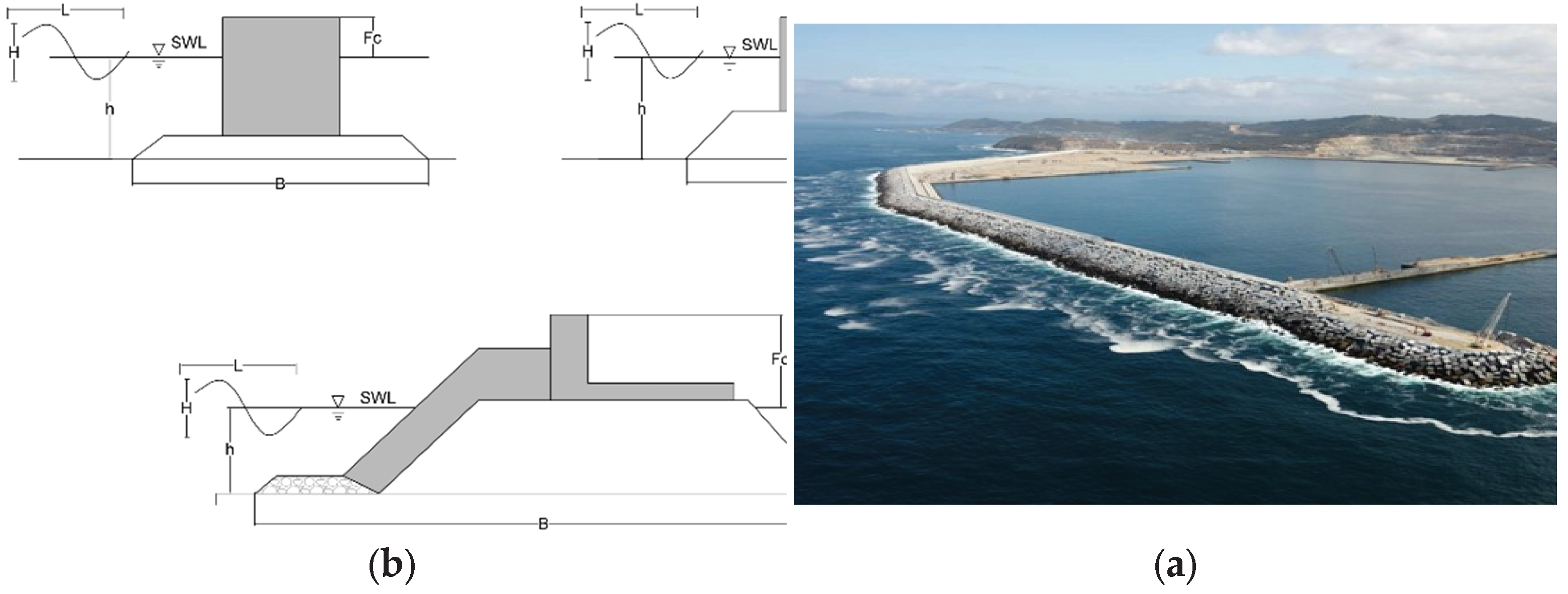
Figure 2.
Overtopping example. Outer port of Punta Langosteira, A Coruña, Spain.
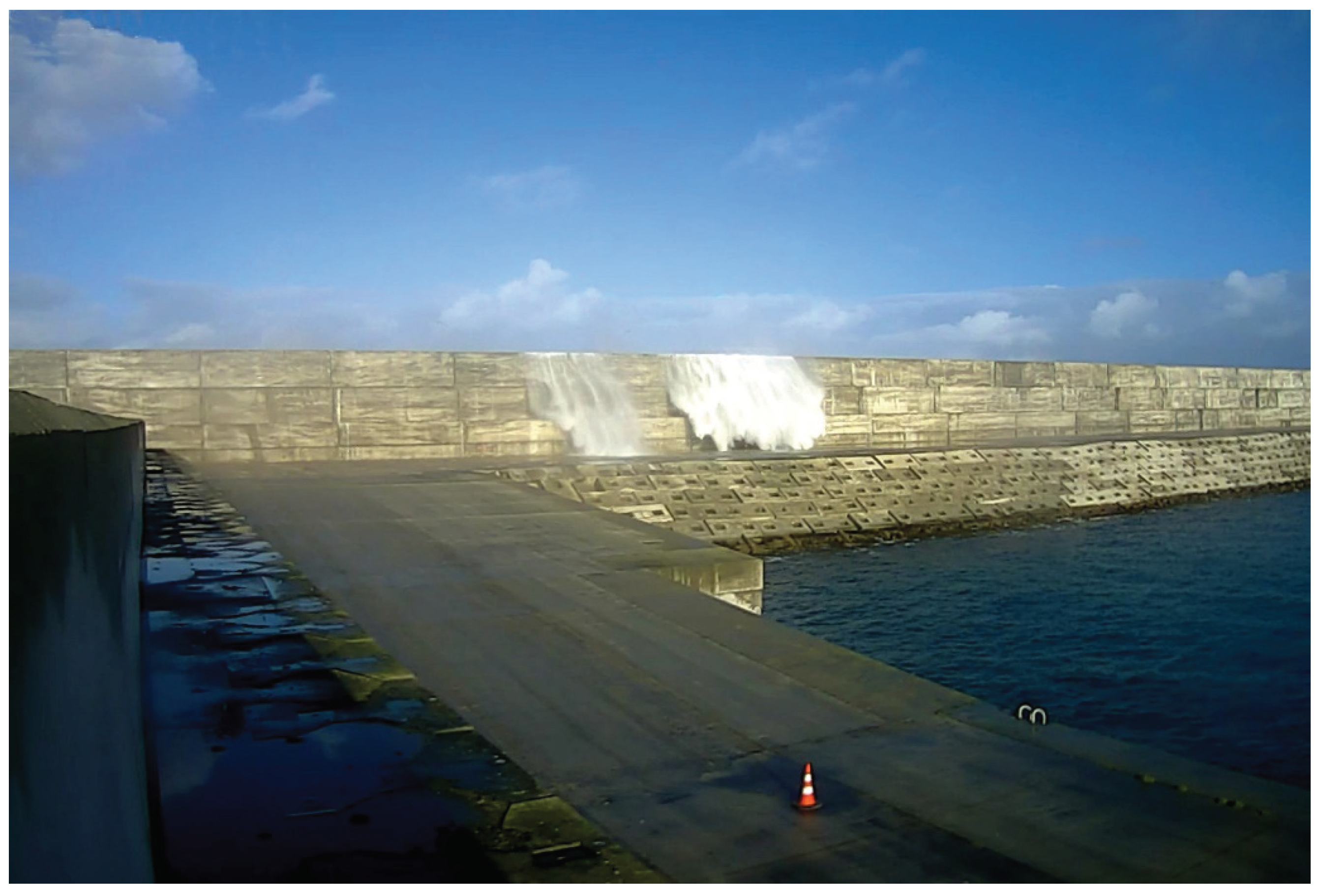
Figure 3.
PR curves for the wave overtopping models using the training datasets.
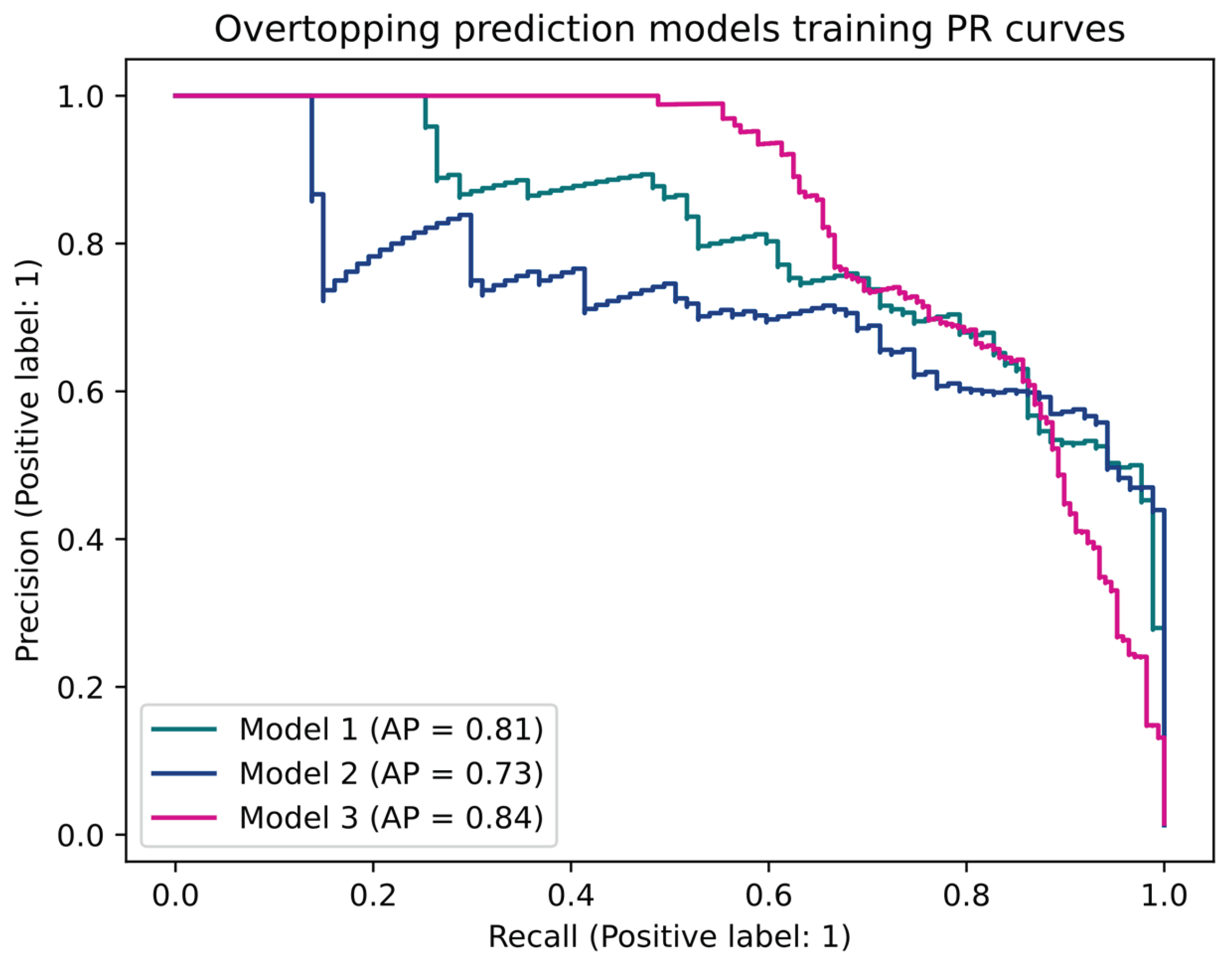
Figure 4.
PR curves for the wave overtopping models using the testing dataset.
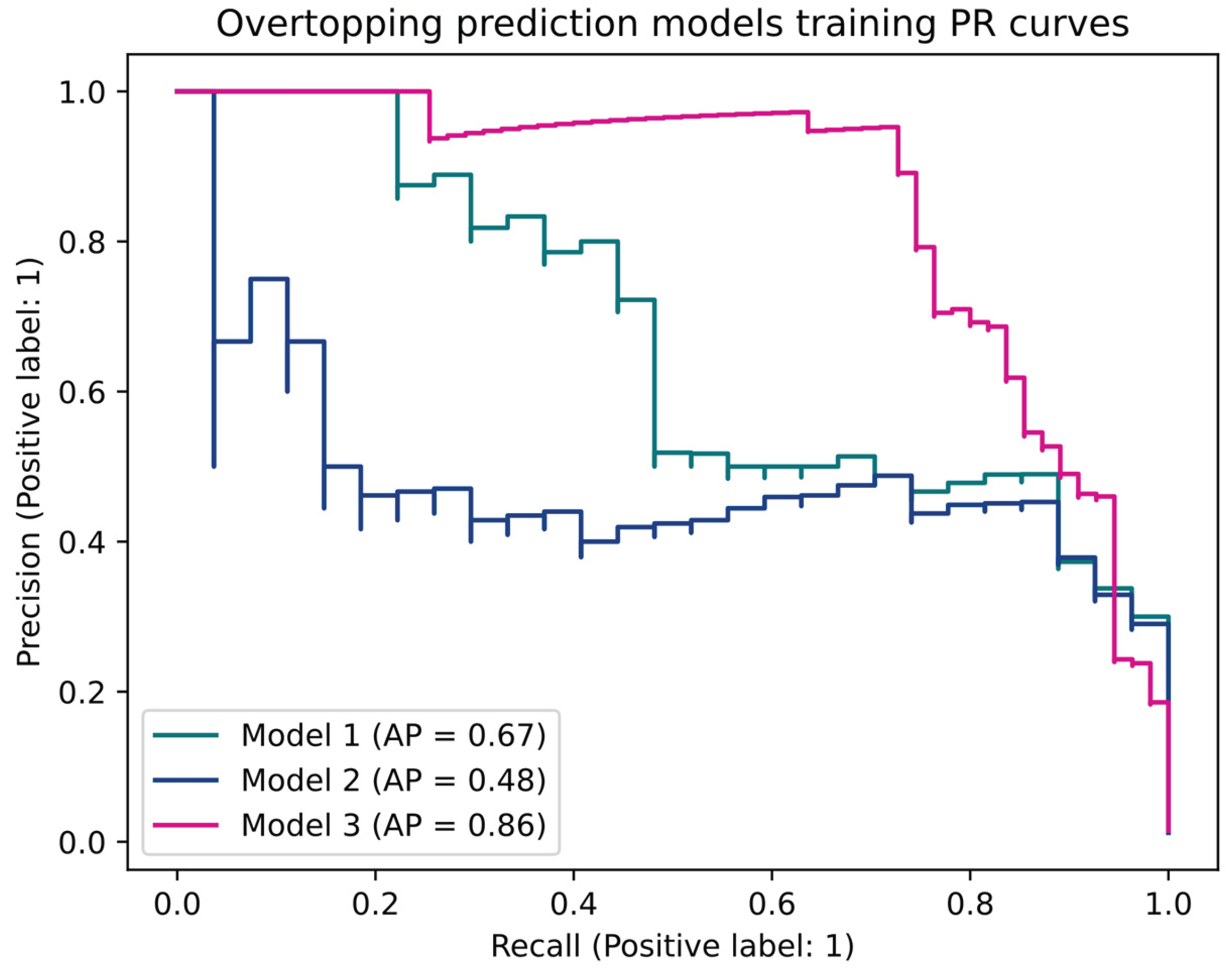
Figure 5.
PR curves for the wave overtopping models 1 and 3 using the testing dataset of model 3 (historical forecasted data).
Figure 5.
PR curves for the wave overtopping models 1 and 3 using the testing dataset of model 3 (historical forecasted data).


Table 1.
Wave overtopping datasets: available data for each dataset (real and predicted data) and purpose (training or testing).
Table 1.
Wave overtopping datasets: available data for each dataset (real and predicted data) and purpose (training or testing).
| Training (h) | Testing (h) | |||
| Dataset | Overtopping | No overtopping | Overtopping | No overtopping |
| Real data without hmax | 6,656 | 87 | 2,219 | 27 |
| Real data with hmax | 6,656 | 87 | 2,219 | 27 |
| Predicted data | 11,131 | 168 | 3,710 | 55 |
Table 2.
Iterative grid-based training process algorithm pseudocode.
| do manually define grid of model hyperparameters for each dataset do for each grid cell (model) do for each resampling iteration do hold-out specific samples using stratified k-fold fit model on the remainder calculate performance on hold-out samples using metric end calculate average performance across hold-out predictions end end determine best hyperparameter fit final model (best hyperparameter) to all training data while error >= ε evaluate final model performance in test set |
Table 3.
Wave overtopping best models’ hyperparameters for several metrics.
| Hyperparameter | |||||||||
|---|---|---|---|---|---|---|---|---|---|
| Model | Metric | Metric value |
Neurons per layer |
Kernel init. |
Iter. | Drop. ratio |
Weight constraint |
lr | Batch size |
| 1 | Precision | 0.77 | 256, 128 | He uniform | 1,000 | 0.25 | 1 | 0.00001 | 1,000 |
| Recall | 0.81 | 256, 128, 64 | He uniform | 1,500 | 0.38 | 1 | 0.00001 | 1,000 | |
| F1 | 0.65 | 256, 256 | He uniform | 1,500 | 0.38 | None | 0.00001 | 1,000 | |
| AP | 0.81 | 256, 128, 64 | He uniform | 1,000 | 0.50 | None | 0.00010 | 1,000 | |
| 2 | Precision | 0.8 | 128, 64, 32 | He uniform | 1,000 | 0.38 | 3 | 0.00001 | None |
| Recall | 0.8 | 256, 128, 64 | He uniform | 1,000 | 0.38 | 1 | 0.00001 | 500 | |
| F1 | 0.69 | 256, 128, 64 | He uniform | 500 | 0.38 | 1 | 0.00001 | 500 | |
| AP | 0.81 | 128, 64, 32 | He uniform | 1,500 | 0.50 | 3 | 0.00010 | 1,000 | |
| 3 | Precision | 1 | 128, 64, 32 | He uniform | 1,000 | 0.50 | None | 0.00010 | 1,000 |
| Recall | 0.74 | 256, 128, 64 | He uniform | 1,000 | 0.38 | None | 0.00001 | 1,000 | |
| F1 | 0.68 | 128, 64, 32 | He uniform | 1,500 | 0.25 | None | 0.00001 | 500 | |
| AP | 0.82 | 128, 64, 32 | He uniform | 1,500 | 0.25 | None | 0.00001 | 500 | |
Table 4.
Confusion matrices for the three wave overtopping models using a 0.25, 0.5, and 0.75 threshold decision boundary on the training data predictions.
Table 4.
Confusion matrices for the three wave overtopping models using a 0.25, 0.5, and 0.75 threshold decision boundary on the training data predictions.
| Predicted | |||||||
|---|---|---|---|---|---|---|---|
| Threshold | 0.25 | 0.5 | 0.75 | ||||
| Model | Real class | No overtop. | Overtop. | No overtop. | Overtop. | No overtop. | Overtop. |
| 1 | No overtop. | 6,496 | 160 | 6,651 | 5 | 6,656 | 0 |
| Overtop. | 1 | 86 | 56 | 31 | 87 | 0 | |
| 3 | No overtop. | 11,027 | 104 | 11,120 | 11 | 11,131 | 0 |
| Overtop. | 22 | 146 | 63 | 105 | 96 | 72 | |
Table 5.
Classification report for the three wave overtopping models using a 0.25, 0.5, and 0.75 threshold decision boundary on the training data predictions.
Table 5.
Classification report for the three wave overtopping models using a 0.25, 0.5, and 0.75 threshold decision boundary on the training data predictions.
| Precision | Recall | F1 | Accuracy | |||||||||||
| Model | Threshold | 0.25 | 0.50 | 0.75 | 0.25 | 0.50 | 0.75 | 0.25 | 0.50 | 0.75 | 0.25 | 0.50 | 0.75 | Support |
| 1 | No overtop. | 1.00 | 0.99 | 0.99 | 0.98 | 1.00 | 1.00 | 0.99 | 1.00 | 0.99 | 6.656 | |||
| Overtop. | 0.35 | 0.86 | 0.00 | 0.99 | 0.36 | 0.00 | 0.52 | 0.50 | 0.00 | 87 | ||||
| Macro avg | 0.67 | 0.93 | 0.49 | 0.98 | 0.68 | 0.50 | 0.75 | 0.75 | 0.50 | 0.98 | 0.99 | 0.99 | 6.743 | |
| Weigh. avg | 0.98 | 0.99 | 0.97 | 0.98 | 0.99 | 0.99 | 0.98 | 0.99 | 0.98 | 6.743 | ||||
| 2 | No overtop. | 1.00 | 0.99 | 0.99 | 0.99 | 1.00 | 1.00 | 0.99 | 0.99 | 0.99 | 6.656 | |||
| Overtop. | 0.47 | 0.00 | 0.00 | 0.99 | 0.00 | 0.00 | 0.64 | 0.00 | 0.00 | 87 | ||||
| Macro avg | 0.73 | 0.49 | 0.49 | 0.99 | 0.50 | 0.50 | 0.81 | 0.50 | 0.50 | 0.99 | 0.99 | 0.99 | 6.743 | |
| Weigh. avg | 0.99 | 0.97 | 0.97 | 0.99 | 0.99 | 0.99 | 0.99 | 0.98 | 0.98 | 6.743 | ||||
| 3 | No overtop. | 1.00 | 0.99 | 0.99 | 0.99 | 1.00 | 1.00 | 0.99 | 1.00 | 1.00 | 11.131 | |||
| Overtop. | 0.58 | 0.91 | 1.00 | 0.87 | 0.62 | 0.43 | 0.70 | 0.74 | 0.60 | 168 | ||||
| Macro avg | 0.79 | 0.95 | 1.00 | 0.93 | 0.81 | 0.71 | 0.85 | 0.87 | 0.80 | 0.99 | 0.99 | 0.99 | 11.299 | |
| Weigh. avg | 0.99 | 0.99 | 0.99 | 0.99 | 0.99 | 0.99 | 0.99 | 0.99 | 0.99 | 11.299 | ||||
Table 6.
Confusion matrices for the three wave overtopping models using a 0.25, 0.5, and 0.75 threshold decision boundary on the testing data predictions.
Table 6.
Confusion matrices for the three wave overtopping models using a 0.25, 0.5, and 0.75 threshold decision boundary on the testing data predictions.
| Predicted | |||||||
|---|---|---|---|---|---|---|---|
| Threshold | 0,25 | 0,5 | 0,75 | ||||
| Model | Real class | No overtop. | Overtop. | No overtop. | Overtop. | No overtop. | Overtop. |
| 1 | No overtop. | 2.162 | 57 | 2.217 | 2 | 2.219 | 0 |
| Overtop. | 1 | 26 | 19 | 8 | 27 | 0 | |
| 2 | No overtop. | 2.191 | 28 | 2.219 | 0 | 2.219 | 0 |
| Overtop. | 4 | 23 | 27 | 0 | 27 | 0 | |
| 3 | No overtop. | 3.670 | 40 | 3.708 | 2 | 3.709 | 1 |
| Overtop. | 8 | 47 | 15 | 40 | 29 | 26 | |
Table 7.
Classification report for the three wave overtopping models using a 0.25, 0.5, and 0.75 threshold decision boundary on the testing data predictions.
Table 7.
Classification report for the three wave overtopping models using a 0.25, 0.5, and 0.75 threshold decision boundary on the testing data predictions.
| Precision | Recall | F1 | Accuracy | |||||||||||
|---|---|---|---|---|---|---|---|---|---|---|---|---|---|---|
| Model | Threshold | 0.25 | 0.50 | 0.75 | 0.25 | 0.50 | 0.75 | 0.25 | 0.50 | 0.75 | 0.25 | 0.50 | 0.75 | Support |
| 1 | No overtop. | 1.00 | 0.99 | 0.99 | 0.97 | 1.00 | 1.00 | 0.99 | 1.00 | 0.99 | 2.219 | |||
| Overtop. | 0.31 | 0.80 | 0.00 | 0.96 | 0.30 | 0.00 | 0.47 | 0.43 | 0.00 | 27 | ||||
| Macro avg | 0.66 | 0.90 | 0.49 | 0.97 | 0.65 | 0.50 | 0.73 | 0.71 | 0.50 | 0.97 | 0.99 | 0.66 | 0.90 | |
| Weigh. avg | 0.99 | 0.99 | 0.98 | 0.97 | 0.99 | 0.99 | 0.98 | 0.99 | 0.98 | 2.246 | ||||
| 2 | No overtop. | 1.00 | 0.99 | 0.99 | 0.99 | 1.00 | 1.00 | 0.99 | 0.99 | 0.99 | 2.219 | |||
| Overtop. | 0.45 | 0.00 | 0.00 | 0.85 | 0.00 | 0.00 | 0.59 | 0.00 | 0.00 | 27 | ||||
| Macro avg | 0.72 | 0.49 | 0.49 | 0.92 | 0.50 | 0.50 | 0.79 | 0.50 | 0.50 | 0.99 | 0.99 | 0.72 | 0.49 | |
| Weigh. avg | 0.99 | 0.98 | 0.98 | 0.99 | 0.99 | 0.99 | 0.99 | 0.98 | 0.98 | 2.246 | ||||
| 3 | No overtop. | 1.00 | 1.00 | 0.99 | 0.99 | 1.00 | 1.00 | 0.99 | 1.00 | 1.00 | 3.710 | |||
| Overtop. | 0.54 | 0.95 | 0.96 | 0.85 | 0.73 | 0.47 | 0.66 | 0.82 | 0.63 | 55 | ||||
| Macro avg | 0.77 | 0.97 | 0.98 | 0.92 | 0.86 | 0.74 | 0.83 | 0.91 | 0.82 | 0.99 | 1.00 | 0.77 | 0.97 | |
| Weigh. avg | 0.99 | 1.00 | 0.99 | 0.99 | 1.00 | 0.99 | 0.99 | 1.00 | 0.99 | 3.765 | ||||
Table 8.
Confusion matrices for the wave overtopping models 1 and 3 using a 0.25, 0.5, and 0.75 threshold on the predictions over the testing dataset of model 3.
Table 8.
Confusion matrices for the wave overtopping models 1 and 3 using a 0.25, 0.5, and 0.75 threshold on the predictions over the testing dataset of model 3.
| Predicted | |||||||
|---|---|---|---|---|---|---|---|
| Threshold | 0,25 | 0,5 | 0,75 | ||||
| Model | Real class | No overtop. | Overtop. | No overtop. | Overtop. | No overtop. | Overtop. |
| 1 | No overtop. | 3.625 | 85 | 3.709 | 1 | 3.710 | 0 |
| Overtop. | 6 | 49 | 40 | 15 | 55 | 0 | |
| 3 | No overtop. | 3.670 | 40 | 3.708 | 2 | 3.709 | 1 |
| Overtop. | 8 | 47 | 15 | 40 | 29 | 26 | |
Table 9.
Classification report for the three wave overtopping models using a 0.25, 0.5, and 0.75 threshold decision boundary on the testing data predictions.
Table 9.
Classification report for the three wave overtopping models using a 0.25, 0.5, and 0.75 threshold decision boundary on the testing data predictions.
| Precision | Recall | F1 | Accuracy | |||||||||||
|---|---|---|---|---|---|---|---|---|---|---|---|---|---|---|
| Mod. | Threshold | 0.25 | 0.50 | 0.75 | 0.25 | 0.50 | 0.75 | 0.25 | 0.50 | 0.75 | 0.25 | 0.50 | 0.75 | Support |
| 1 | No overtop. | 1.00 | 0.99 | 0.99 | 0.98 | 1.00 | 1.00 | 0.99 | 0.99 | 0.99 | 3.710 | |||
| Overtop. | 0.37 | 0.94 | 0.00 | 0.89 | 0.27 | 0.00 | 0.52 | 0.42 | 0.00 | 55 | ||||
| Macro avg | 0.68 | 0.96 | 0.49 | 0.93 | 0.64 | 0.50 | 0.75 | 0.71 | 0.50 | 0.98 | 0.99 | 0.99 | 3.765 | |
| Weigh. avg | 0.99 | 0.99 | 0.97 | 0.98 | 0.99 | 0.99 | 0.98 | 0.99 | 0.98 | 3.765 | ||||
| 3 | No overtop. | 1.00 | 1.00 | 0.99 | 0.99 | 1.00 | 1.00 | 0.99 | 1.00 | 1.00 | 3.710 | |||
| Overtop. | 0.54 | 0.95 | 0.96 | 0.85 | 0.73 | 0.47 | 0.66 | 0.82 | 0.63 | 55 | ||||
| Macro avg | 0.77 | 0.97 | 0.98 | 0.92 | 0.86 | 0.74 | 0.83 | 0.91 | 0.82 | 0.99 | 1.00 | 0.99 | 3.765 | |
| Weigh. avg | 0.99 | 1.00 | 0.99 | 0.99 | 1.00 | 0.99 | 0.99 | 1.00 | 0.99 | 3.765 | ||||
Disclaimer/Publisher’s Note: The statements, opinions and data contained in all publications are solely those of the individual author(s) and contributor(s) and not of MDPI and/or the editor(s). MDPI and/or the editor(s) disclaim responsibility for any injury to people or property resulting from any ideas, methods, instructions or products referred to in the content. |
© 2024 by the authors. Licensee MDPI, Basel, Switzerland. This article is an open access article distributed under the terms and conditions of the Creative Commons Attribution (CC BY) license (http://creativecommons.org/licenses/by/4.0/).
Copyright: This open access article is published under a Creative Commons CC BY 4.0 license, which permit the free download, distribution, and reuse, provided that the author and preprint are cited in any reuse.


