Submitted:
21 February 2024
Posted:
21 February 2024
You are already at the latest version
Abstract
Sustainable continuous cover forestry is defined and analyzed in several ways. The differential
equation representing growth of the basal areas of individual trees, motivated by fundamental
biological production theory by Lohmander (2017a), is analyzed and extended in different directions.
From the solution of the differential equation, the basal area and the tree diameter are obtained as
explicit functions of time. The diameter is a strictly increasing function of time. In the absence of
competitors, the diameter increment is shown to be a strictly decreasing function of time. Hence, the
diameter increment can also be interpreted as a strictly decreasing function of the diameter. Alternative
forms of adjustment of the differential equation, with consideration of competition, are defined. If the
competition is strong, with large trees in the vicinity of a particular tree, then the basal area increment,
and the diameter increment, are reduced. The growth of a large tree is less sensitive than the growth of
a small tree, to competition from other trees. Under strong competition, the basal area increment, and
the diameter increment, are strictly concave functions of the size of the tree. The unique maximum of
the diameter increment occurs at a higher diameter, if the competition increases. In dynamic
equilibrium, the tree size frequency distribution is stationary. If natural tree mortality can be avoided
via the harvest strategy, the tree size frequency distribution is a function of the size and competition
dependent growth function, and the harvest strategy. Empirical tree size frequency data are used to
simultaneously estimate parameters of a size and competition dependent growth function and the
applied harvest strategy, via nonlinear optimization. The properties of the estimated growth function
are consistent with the corresponding properties of the production theoretically motivated hypothetical
function, and the properties of the estimated harvest strategy confirm the corresponding hypotheses.
The R2 of the nonlinear regression exceeds 0.97. With access to an empirically estimated equilibrium
tree size distribution, it is possible to: 1. Estimate size frequency relevant parameters of tree size and
competition dependent growth functions for individual trees. 2. Estimate the applied harvest strategy.
3. Explain and reproduce the empirically estimated tree size equilibrium distribution.
Keywords:
sustainable forestry
; sustainability
; continuous cover forestry
; size distribution
; forest dynamics
; optimization
; estimation
Introduction
Sustainable forests and forestry are central components of a sustainable world. They contribute to continuous flows of forest products such as building materials and fuels, and valuable environmental conditions, necessary for large amounts of species, all over planet Earth. Simultaneously, growing forests absorb CO2 from the atmosphere, as an input in the photosynthesis growth process, which reduces global warming.
CCF, Continuous Cover Forestry:
With Continuous Cover Forestry, CCF, the forests always contain trees. Clear- cuts never take place. CCF forests do not only give continuous flows of forest products and economic results. CCF forests also continuously and sustainably absorb CO2 from the atmosphere, and water from extreme rains, reducing global warming and the impacts of floods.
Haight (1987) compares CCF and forestry with clear cuts. He finds that, in general, constrained management regimes that involve clearcutting and planting are suboptimal relative to the optimal solution to the more general investment model, which may involve selection harvesting and uneven-aged management. Lohmander (1987) determines economically optimal principles of forest management under the influence of stochastic prices, random growth, and disturbances, such as storms and wind- throws. Lohmander (1988a), Lohmander (1988b) and Lohmander & Helles (1987), give central insights to these stochastic adaptive optimization problems and the effects on sustainable and economically rational forest management. Schütz (2006) models the dynamics of deterministic continuous cover forestry, CCF, in a mathematically consistent way that ties several central decision problems together, including harvesting and regeneration. Explicit economic optimization of the decisions is however missing. Empirical data from beech forests in Eastern Germany are used to estimate some of the functions. Pukkala, Lähde & Laiho (2010) and Tahvonen, Pukkala et al. (2010) explicitly and deterministically optimize the forest structure and management of CCF forests in Finland and Tahvonen and Rämö (2016) compare continuous cover forestry to forestry with clear-cuts. They report that the economically optimal choice of forestry method depends on the initial stand state, site productivity, the market rate of interest and other factors such as the cost of artificial regeneration. Hessenmöller et al (2018) develop a deterministic silvicultural strategy for beech forests. The articles by Schütz (2006) and Hessenmöller et al (2018) concern the same species and the same geographical forest region in Germany. The planning approach by Hessenmöller et al (2018), however, is based on target diameters, subjectively determined by the land owners. From an economic point of view, a fundamental problem is that economic optimization is not applied when the forestry strategy is developed. Furthermore, the projected canopy area of a tree is modeled as a function only of the basal area of that tree. This function is applied to determine targets for stand based volumes, basal areas, and stem densities at “full canopy cover”. However, the canopy area of a tree is dynamically affected by spatial competition from other trees. This has been empirically investigated in detail, and reported in recent articles by Wang, Ge, Hou et al. (2021), and by Hou and Chai (2022). Hence, a tree with a particular basal area, may have a small canopy area in a dense forest and a large canopy area in a less dense forest. Since the canopy area is dynamically affected by forest management decisions, such as harvesting, a canopy area function cannot logically be considered as independent of competition, and used to optimize forest harvests and other management decisions. The approach by Schütz (2006), developed for the same geographical area and species, does not suffer from these methodological canopy problems. For these reasons, the author of this paper recommends that the theoretically and empirically consistent models by Schütz (2006), updated with economic optimization, are applied to manage the beech forests of Eastern Germany.
CCF and a sustainable planet Earth:
Some of the key problems, with respect to the sustainability of planet Earth, concern global warming, forest fires, and biodiversity.
Lohmander (2020a) derives some fundamental principles of optimal forest utilization with consideration of global warming: If the average forest harvesting level is proportional to the area under active forest management, and if the area of active forest management increases, then the area covered by forests in dynamic equilibria with net CO2 absorption close to zero, decreases. Hence, the absorbed amount of CO2 per time unit, is an increasing function of the sustainable forest harvesting level. To decrease global warming, we should increase sustainable harvesting, via an increasing area of actively managed CCF forests. Lohmander (2020b) develops a numerical model and derives explicit results based on the general findings in Lohmander (2020a): If the relative weight of the utility of the climate increases, and we desire a cooler climate, then the optimal area of natural forests that should be transformed to managed continuous cover forests increases. If 600 M hectares are transformed during 60 years, from 2020 until 2080, then the concentration of CO2 in the atmosphere can be reduced by 8 ppm until the year 2100, compared to the situation without forestry expansion. Strong global industrial net emission reductions are however also necessary, if we are interested to efficiently stop global warming. To reduce the expected negative effects of forest fires, several methods can and should be combined. Lohmander (2021a) optimizes combinations of adjustments of forestry decisions, affecting stock levels, infrastructure, such as road network density, and fire management. Often, the most efficient ways to solve a problem, include combinations of several methods. The global warming problem, for instance, can be solved via optimal combinations of emission reductions and expansion of sustainable forestry. This is reported by Lohmander (2022a) and (2022b), where also a global CO2 model is defined, based on official atmospheric CO2 data series and dynamic global emission data. The future consequences of alternative global emission reduction levels, and forestry expansion strategies, are calculated and presented. Market forces may be used to partly control the climate via forestry decisions, since forestry decisions are affected by CO2 related subsidies. Mohammadi, Lohmander et al (2023) derive the general principles of global warming reduction via such forestry-CO2 subsidies.
Understanding and predicting CCF growth:
It is necessary to understand the fundamental principles of how trees grow in CCF forests, and how the growth can be affected by different kinds of forestry decisions. Without such knowledge, continuous and sustainable forestry cannot be optimized. It is also necessary to statistically estimate the growth function parameters to obtain reliable numerical models, that can be used to develop practically relevant guidelines.
Mohammadi, Lohmander and Olsson (2017) analyze the dynamics of multi species forests with alternative kinds of simplified growth functions. A general dynamic function for the basal area of individual trees is derived by Lohmander (2017a). This is based on a production theoretically motivated autonomous differential equation. The growth function is empirically estimated, in different countries and with several tree species. Mohammadi, Mohammadi et al (2017) find that a version of the Lohmander (2017a) model with competition adjustment, explains the basal area growth in uneven-aged Caspian mixed species forests better than alternative models. Hatami, Lohmander et al (2018) estimate basal area growth functions for several tree species in CCF forests in Iran, via the Lohmander (2017a) differential equation with competition correction. Fagerberg, Olsson, Lohmander et al (2022b) estimate similar Lohmander (2017a) models for Norway spruce, in Sweden, with and without competition adjustment functions. Fagerberg, Lohmander et al (2022a) compare these models to other kinds of models, and discover that the Lohmander (2017a) model gives more reliable predictions than the other tested models.
Optimization approaches:
Strategies can be motivated as rational if they lead to the best possible decisions and results. The best possible results are optimal solutions. Hence, we always need optimization when strategies should be developed.
Applied optimization is the key to operations research. Lohmander (2018a) includes general approaches and applications of mathematical modeling in operations research. New theoretical extensions are given, with focus on stochastic dynamic problems with large numbers of dimensions. Stochastic dynamic programming with Markov chains, applied to forest sector optimization including CCF, is presented in Lohmander and Mohamadi (2017).
Climate changes, market prices, pests, and other stochastic disturbances, cannot be perfectly predicted over long planning horizons. This has often been forgotten, and/or neglected, in forestry planning. It is very important to be able to respond optimally to changing and unpredictable future events. Such optimization is called Adaptive Optimization, AO. Two approaches to optimal adaptive control under large dimensionality, are presented in Lohmander (2017b), and control function optimization for stochastic continuous cover forest management decisions is described in Lohmander (2019a).
Optimization of CCS:
Optimal CCF is per definition the best CCF.
Lohmander (1992) shows how optimization of an adaptive control function can be used to optimize the economics of CCF forestry, under the influence of stochastic prices. The adaptive stock control function is optimized via a numerical stochastic quasi-gradient method. The optimal spatial stochastic dynamic CCF control problem, based on a growth function of the type presented in Schütz (2006), and a stochastic control function, according to the principles derived in Lohmander (2017b), is found in Lohmander (2018b). The optimization method is also combined with a growth function of the Lohmander (2017a) type and stochastic prices, in Lohmander (2019b), where a market adaptive control function for CCF, that also considers spatially explicit competition between trees, is developed.
Lohmander (2021b) and Lohmander and Fagerberg (2022) demonstrate how the forestry decisions in a Swedish case study based on the tree species Picea abies, can be optimized, using the Lohmander (2019b) approach in combination with detailed empirical information about the initial positions and properties of all individual trees. Optimal adaptive rules are defined and determined, that show how the harvest decisions are affected by the properties of the individual trees and the degrees of competition. Optimal decisions are functions of many parameters, some of which are very difficult, or practically impossible, to predict over long horizons. Future prices of timber of different log dimensions and qualities, rates of interest, future qualities of logs etc., costs of operations with future machinery, access to and wages of future labor, etc. are simply not known today. Still, efforts are made to predict things such as future log qualities, which is illustrated by Fagerberg et al (2023).
Structure of the analysis:
A tree size distribution can be considered and understood as a function of all the processes that affect forests and individual trees, such as growth processes of individual trees, regeneration of plants, harvesting and competition. In the following analysis, these questions will be asked and answered:
Is it possible to start from an empirically estimated equilibrium tree size distribution, and
- to estimate parameters of a tree size and competition dependent growth function for individual trees?
- to estimate the applied harvest strategy?
- to explain and reproduce the empirically estimated tree size equilibrium distribution?
- The analysis is divided into the following sections:
- The empirical facts.
- The basal area differential equation and the dynamic properties of the solution.
- The dynamics of trees in size classes.
- Construction of a nonlinear dynamic optimization model.
- Estimation of the model parameters.
Materials and Methods
a. The empirical facts:
Figure 1. shows an empirical estimation of relative frequencies of trees in different diameter classes. The data represents CCF forests with the species Picea abies, in southern Sweden. The detailed background to the data, several statistical analyses and alternative modeling efforts based on these data, can be studied in Fagerberg, Olsson, Lohmander, et al (2022b), and in Fagerberg, Lohmander, et al (2022a). The data in Figure 1. is assumed to represent an empirically estimated tree size distribution in dynamic equilibrium. This data is used to estimate parameters of a tree size and competition dependent growth function for individual trees, and of the applied harvest strategy function. These estimated parameters are simultaneously used to derive an approximation of the empirically estimated tree size equilibrium distribution. The estimated parameters are the results of nonlinear least squares minimization of the deviations between the empirically observed frequencies and the parameter dependent equilibrium frequencies. Hence, a nonlinear full system equilibrium analysis of the interdependent processes is performed.
b. The basal area differential equation and the dynamic properties of the solution:
Lohmander (2017a) gives the theoretical motivation of equation (1), a differential equation representing the dynamics of the basal area of an individual tree, x, without competition. The basal area is the approximately circular horizontal area of the stem, 1.3 meters above the ground level. Equation (1) is motivated by components from biological production theory, photosynthesis, light projection areas and size related efficiency dependences. The parameters a and b are introduced in (1).
Equation (1) can, via the new parameter c, be reformulated to equation (2).
The derivations based on (1) in Lohmander (2017a), give the solution in equation (3).
Via the definition of k in (4), it is possible to transform (3) to equation (5).
Now, we have a more compact version, (5), of the solution to the differential equation (2).
From the definition of the differential equation of the basal area increment, (2), we get (6) and (7).
Equation (7) can be used to determine the sign of k. Compare equation (8).
In the following analysis, we will need to know more about the value of k. In equation (9), we simplify the notation, using the new variable y.
Clearly, from (9), we get (10).
The first order derivative of k with respect to y is (11).
Equations (9), (10) and (12) make sure that k is strictly less than -1 for all strictly positive and relevant values of x. Compare (13). This is essential information in the following derivations.
We introduce one more variable, h, in (14).
Now, in (15), we have a more convenient expression of x(t), compared to equation (5). Note the following, for strictly positive values of t, concerning equation (15): The fact that k < -1, from (13), makes sure that the nominator avoids the number zero, and always is strictly positive. Furthermore, the fact that k < 0, from (8), makes sure that also the denominator avoids the number zero, and always stays strictly positive.
The basal area of the individual tree is a function the radius, r, which is a function of time (16).
The radius function of time (17), is obtained via a transformation of the basal area function of time (16). Equations (8) and (13) guarantee that r(t) > 0 for t > 0.
In the following analysis, it is important to know how the radius, and the diameter, change over time. The growth of the radius is the derivative of the radius with respect to time (18).
(18) can be simplified to (19).
Since we have information about the signs of relevant parameters, we can instantly determine that the radius increment is strictly positive (20).
Later in this analysis, it is shown how the sign of the change of the radius increment over time, influences the properties of the equilibrium diameter frequency distribution. For this reason, we investigate the second order derivative of the radius increment with respect to time (21).
(21) gives (22) and (23).
Continued transformations give (24), (25) and (26).
Since we already know the signs of several parameters, found in (27), we can show that the radius increment of a tree without competition, is a strictly decreasing function of time. Observe in (27), that it is necessary to know, from (13), that k < -1.
Thus, (27), is a general theoretical result, based on the differential equation (1), which has been rigorously tested and estimated for several species in different countries. Note that Schütz (2006) makes a different growth function assumption, which implies that the radius and diameter increments, without competition, are strictly increasing functions of time (and diameter).
c. The dynamics of trees in size classes:
Forests without harvests and lethal competition:
Consider a forest with trees in different size classes, i. The size, for instance “diameter” 1.3 meters above ground, of a tree, is a strictly increasing function of the size class index, i. Let ni denote the number of trees in size class i. gi is the share of the trees in size class i that grow to the next size class, i+1, per time unit. In this subsection, we assume that the tree mortality and the harvest levels are zero. Equation (28) gives the time derivative, in Newtonian notation, of the number of trees in size class i. Clearly, new trees grow to size class i, from the lower size class, i-1, and some trees leave size class i, and grow to the higher size class, i+1.
Equation (29) shows the links between three different size classes. Note that (29) does not include all size classes, just three such classes. Lower and higher size classes may also exist. Furthermore, size classes can be defined in different ways, for instance representing 1 cm diameter classes, 5 cm classes or classes of some other size.
Now, we consider a forest where the numbers of trees in different size classes do not change over time. This means that the tree size frequency distribution is in dynamic equilibrium. This is illustrated in (30).
Equation (30) implies (31).
The number of trees that enter a size class is equal to the number of trees that leave the same size class (32).
(33) follows from (32) and means that the number of trees per size class is a strictly decreasing function of the size class index, in case the share of trees that grow to the next size class per time unit is a strictly increasing function of the size class index.
Empirical observation:
The number of trees per diameter class is a strictly decreasing function of the diameter, except for in one case, which is assumed to be a random deviation from the principle. Compare Figure 1.
Mathematical observation:
The number of trees per diameter class is a strictly decreasing function of the diameter in case the diameter increment is a strictly increasing function of the diameter. Furthermore, since the diameter is a strictly increasing function of time: The number of trees per diameter class is a strictly decreasing function of the diameter in case the diameter increment is a strictly increasing function of the age of the tree (which is an increasing function of time). The general mathematical growth function with very strong empirical support, has however shown that the diameter increment of trees without competition is a strictly decreasing function of time. Compare equation (27).
General observation:
Consider a forest, during a period without harvesting and mortality. Then, if the number of trees per diameter class is a strictly decreasing function of the diameter, then the diameter increment is a strictly increasing function of the diameter of the tree (which is an increasing function of the age of the tree, and time). This means that competition between trees affects the growth in a way such that the diameter growth of small trees is strictly more reduced than the diameter growth of large trees. This will also be demonstrated in the next steps of analysis in this paper.
Forests with harvests and competition:
Now, we also consider harvesting and competition between trees. Gi is the share of the trees in size class i that grow to the next size class, i+1, per time unit, under the influence of competition from other trees. Observe that the diameter interval of a diameter class, and the length of a time unit, have not been specified in this general section. Hence, tree size frequency distributions do not reveal the absolute levels of forest production per year.
Equation (34) shows the time derivative of the number of trees in size class i, as a function of the number of trees in the lower size class, ni-1, the shares of the trees in the two size classes, that grow to the next size classes, Gi-1 and Gi, and ui, the share of the trees in size class i that are harvested before they reach the next size class.
In dynamic equilibrium, the numbers of trees in the different size classes do not change over time. Equations (35) and 36 are satisfied.
From equation (36), we get (37).
Observation:
We already know from equation (27) that, without competition, the diameter increment is a strictly decreasing function of time, and indirectly, of the diameter class. Hence, gi > gi+1 . However, if competition from other trees in the forest reduces the diameter increments of small trees more than it reduces the diameter increments of large trees, it is possible that Gi < Gi+1 , even if gi > gi+1 . Equation (37) means that it is quite possible that the relative frequency of trees is a strictly decreasing function of the diameter class index i, as we see in Figure 1, even if the trees in a size class are small and no trees are harvested, which means that ui+1 = 0. Equation (37) also shows that the relative frequency of trees is a more rapidly decreasing function of the size class index i, if the share of trees that are harvested, ui+1, increases.
d. Construction of a nonlinear dynamic optimization model:
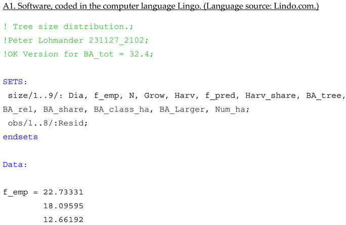
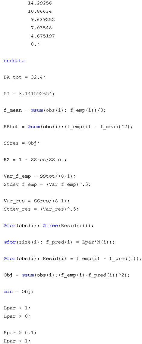
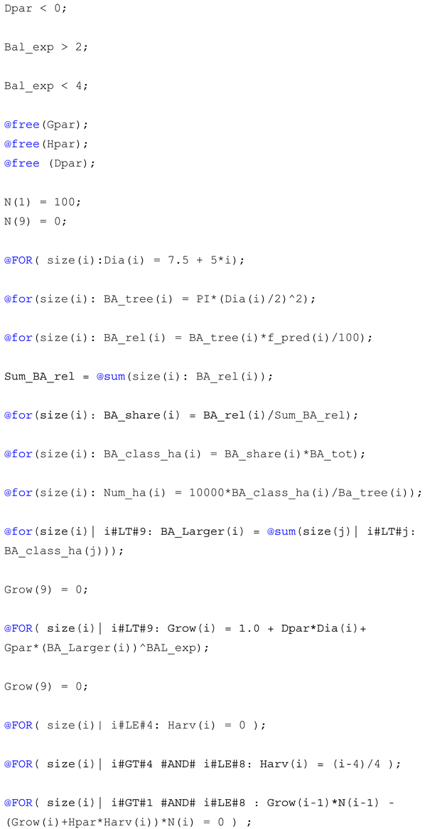
A numerical model is constructed. This is based on the discoveries and observations presented in the earlier sections. The complete numerical model is included in the Appendix A. In this section, the key equations and variables are motivated and presented in detail. Size classes are defined as diameter classes, consistent with the classes of the empirical data presented in Figure 1. Equation (38) corresponds to Equation (35). Equation (38) also specifies the values of the diameter class indices, i, that are relevant in the optimization model. Furthermore, is introduced as an optimized parameter (variable, during the optimization), that is multiplied by the diameter class dependent harvest trend parameters wi, defined in (40), to give the harvest shares ui.
As illustrated and derived in Lohmander & Fagerberg (2022), the probability that it is optimal to harvest a particular tree, is an increasing function of the diameter of that tree, if the diameter is sufficiently large, and zero for smaller trees. Hence, one hypothesis is that the optimized value of is strictly positive. wi is a strictly increasing function of the diameter class, for large diameters, and zero for smaller diameters. In the numerical model, the notation is partly different. Equation (38) corresponds to equation (39) in the numerical model.
@FOR( size(i)| i#GT#1 #AND# i#LE#8 :
Grow(i-1)*N(i-1) – (Grow(i)+Hpar*Harv(i))*N(i) = 0 )
Grow(i-1)*N(i-1) – (Grow(i)+Hpar*Harv(i))*N(i) = 0 )
Equation (40) corresponds to equation (41) in the numerical model.
@FOR( size(i)| i#LE#4: Harv(i) = 0 );
@FOR( size(i)| i#GT#4 #AND# i#LE#8: Harv(i) = (i-4)/4 );
Harv(9) = 1;
@FOR( size(i)| i#GT#4 #AND# i#LE#8: Harv(i) = (i-4)/4 );
Harv(9) = 1;
Equation (42) specifies Gi as a function of the diameter, 2ri, and the basal area per hectare of larger trees, . Equation (42) introduces three parameters (treated as variables, during the optimization), that are optimized, namely , and .
Equation (42) corresponds to equation (43) in the numerical model.
@FOR( size(i)| i#LT#9: Grow(i) = 1.0 + Dpar*Dia(i)+ Gpar*(BA_Larger(i))^BAL_exp)
@FOR( size(i)| i#LT#9: Grow(i) = 1.0 + Dpar*Dia(i)+ Gpar*(BA_Larger(i))^BAL_exp)
The estimated parameters determine several functions, that together determine the relative equilibrium frequencies of trees in different size classes. To determine the numbers of trees in different size classes per hectare, the basal area per size class and hectare, and the basal area of larger trees per hectare and size class, it is also necessary to utilize estimates of the total basal area per hectare. This is done in the numerical model in the Appendix A.
To transform the relative size frequency results derived in the numerical model to empirically relevant absolute values, the empirically estimated average total basal area per hectare, 32.4 m2 per hectare, is used. This parameter value is calculated from data found in Fagerberg, Olsson, Lohmander, et al (2022b). In the numerical Appendix A, this is denoted BA_TOT.
e. Estimation of the model parameters:
A nonlinear full system equilibrium analysis of all interdependent processes is performed. When the numerical model in the Appendix A is executed, the problem is solved, and all parameters are determined by the algorithm. The numerical data observations, illustrated in Figure 1., representing the empirically estimated equilibrium tree size distribution, are included in the nonlinear numerical optimization model. These observations are used to estimate the parameters, , , and . These parameter values include the information that we need, about the tree size and competition dependent growth function for individual trees, and of the applied harvest strategy function. The estimated parameters are simultaneously used to derive an approximation of the empirically estimated tree size equilibrium distribution. The estimated parameters are the results of nonlinear least squares minimization of the deviations between the empirically observed frequencies and the parameter dependent equilibrium frequencies.
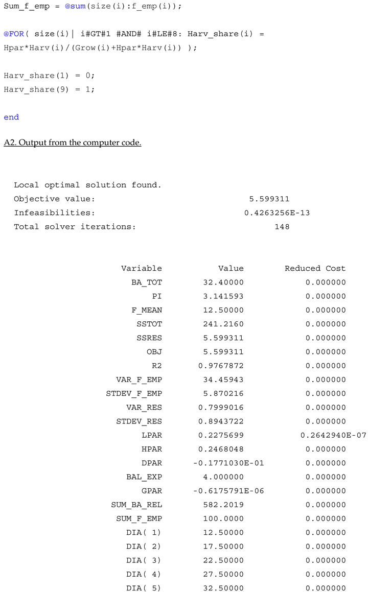
Results
The nonlinear dynamic optimization model, introduced in the earlier section and included in the Appendix A, minimizes the sum of squares of the residuals. The residuals are the relative frequency prediction errors. Table 1 includes key statistics. The residual sum of squares, is approximately 6. This is much smaller than the total sum of squares. The total sum of squares is the sum of the squared deviations of the empirical relative frequencies from the average relative frequencies. That sum exceeds 241. The R2 value, exceeding 0.976, indicates that the model predicts the relative equilibrium frequencies very well.
The standard deviation of the residuals is lower than 0.9 percent units, according to Table 1. This is consistent with the illustration in Figure 2, where all, except for two, of the absolute relative frequency errors are very close to zero. Only in two cases, the absolute relative frequency errors exceed 1 percent unit.
The optimized parameter values are presented in Table 2. The numerical notation is applied in the optimization code in the Appendix A.
We observe that the diameter dependent harvest trend, defined via equations (38) and (40), is reasonable, since the optimal value of in Table 2 is estimated to be strictly positive.
Thanks to the combination of the estimated parameter value , and the diameter class dependent harvest trend, defined in equation (40), it is possible to derive the diameter dependent relative harvest function, found in Figure 3. As explained and derived in Lohmander & Fagerberg (2022), the probability that it is optimal to harvest a particular tree, is an increasing function of the diameter of that tree, if the diameter is sufficiently large, and zero for smaller trees. This is consistent with the optimized results illustrated in Figure 3.
As seen in equation (27), the radius increment of a tree without competition, is a strictly decreasing function of time. This is consistent with the derived result. In Table 2, the optimal value of is really found to be strictly negative. Note that Schütz (2006) makes a different growth function assumption. With the Schütz (2006) assumption, the radius and diameter increments, without competition, are strictly increasing functions of time (and diameter).
The predicted relative frequencies of trees in different diameter classes, shown in Figure 2., combined with the total basal area per hectare, can be used to derive the basal area of trees in different diameter classes, illustrated in Figure 4. In Figure 2., we see that the relative frequency of small diameter trees is much larger than the relative frequency of large diameter trees. Still, since the basal area per tree is very much larger for large diameter trees than for small diameter trees, the basal area of the trees in a diameter class, in Figure 4., is much higher for diameter class 37.5 cm than for diameter class 12.5 cm.
The share of trees that grow to the next diameter class, proportional to the diameter increment, was defined in (42). In (44), the estimated optimal parameter values from Table 2. have been attached to this function. Clearly, if the competition from larger trees would not affect the growth, would be zero, and the diameter increment would be a strictly decreasing function of the diameter. However, as we see in (44), is strictly negative, which means that the diameter increment is strictly negatively affected by competition from larger trees. obtained the value 4, which is higher than the value 3, reported by Schütz (2006). It is likely that the free optimal value of exceeds 4. In the optimization model, a constraint makes sure that is below or equal to 4, since numerical instability sometimes is observed for higher values of . The complete model is found in the Appendix A. The reader is encouraged to investigate alternative specifications in the future.
The basal area of larger trees is derived and found in Figure 5. Note that this is a strictly decreasing function of the diameter class. Since this value is raised to the exponent = 4, and multiplied by a strictly negative parameter, , and included in the diameter growth function, (44), it is clear that trees with small diameters, are much more negatively affected by competition from larger trees, than large diameter trees.
Hence, in continuous cover forests, small trees have small year rings, and stay in the small diameter classes for a long time. This is good for the future quality of the timber, which benefits from small year rings in the center of the logs.
In forests with clear cuts, however, small trees have very limited competition from larger trees. For this reason, they develop large year rings. Mostly, this leads to low quality future timber logs, and low economic values of the timber.
The equilibrium number of stems per hectare, in different diameter classes, is found in Figure 6. This function is the result of all the parameters estimated via the nonlinear regression/optimization model and the empirically estimated basal area per hectare. In Table 2, we also find the estimate of the parameter . This is a scaling parameter, used to adjust the relative frequencies of trees in different diameter classes in the algorithm.
Discussion
Science and intensified research can hopefully make us better understand the facts and processes of relevance to the present and future of our world. Furthermore, with improved understanding, we may control the development of our planet in a sustainable way, with consideration of a relevant objective function.
Rational control of the forests can strongly improve several things of importance to humans and most other animals and plants. Several attempts to optimize forestry with consideration of global warming, production economic results, forest fires etc. have been reported and discussed in the introduction. Forests are also essential to many other dimensions of life, including biodiversity and recreation.
In this paper, we have seen that it is possible to gain fundamental understanding of rather complicated processes, governing the dynamics of the forests, also via data that sometimes can be gathered via simple methods. Sometimes, it is even sufficient to collect empirical tree size frequency data, to derive properties of growth functions, harvesting strategies, and competition mechanisms.
Let us in the future continue the processes that lead to better understanding and more optimal management of our forests. In the process, we can improve not only the global climate, the economic results, and the biodiversity, but also expand international cooperation and avoid wars.
Conclusions
A tree size distribution can be considered and understood as a function of all the processes that affect forests and individual trees, such as growth processes of individual trees, regeneration of plants, harvesting and competition.
In dynamic equilibrium, the tree size frequency distribution is stationary. The tree size frequency distribution is a function of the growth function, competition, and the harvest strategy. In this study, we have assumed that tree mortality is avoided via the harvest strategy decisions.
Nonlinear optimization and empirical tree size frequency data have been used to simultaneously estimate tree size frequency relevant parameters of a diameter growth function with competition dependence, and the harvest strategy. The properties of the estimated growth function are consistent with the theoretically defined function. The properties of the estimated harvest strategy confirm the hypotheses. The R2 of the nonlinear regression exceeds 0.97.
With access to an empirically estimated equilibrium tree size distribution, it is possible to:
- Estimate parameters of tree size and competition dependent growth functions for individual trees.
- Estimate the applied harvest strategy.
- Explain and reproduce the empirically estimated tree size equilibrium distribution.
Appendix A
References
- Fagerberg, N., Lohmander, P., Eriksson, O., Olsson, J-O., Poudel, B.C., & Bergh, J. (2022a). Evaluation of individual-tree growth models for Picea abies based on a case study of an uneven-sized stand in southern Sweden, Scandinavian Journal of Forest Research, 37 (1), 45-58. https://www.tandfonline.com/doi/pdf/10.1080/02827581.2022.2037700. [CrossRef]
- Fagerberg, N., Olsson, J-O., Lohmander, P., Andersson, M., Bergh, J. (2022b). Individual-tree distance-dependent growth models for uneven-sized Norway spruce, Forestry: An International Journal of Forest Research, 2022;, cpac017. [CrossRef]
- Fagerberg, N., Seifert, S., Seifert, T., Lohmander, P., Alissandrakis, A., Magnusson, B., Bergh, J., Adamopoulos, S., Bader, M.K.-F. (2023). Prediction of knot size in uneven-sized Norway spruce stands in Sweden, Forest Ecology and Management, Volume 544, 121206, ISSN 0378-1127, https://www.sciencedirect.com/science/article/pii/S0378112723004401. [CrossRef]
- Haight, Robert. (1987). Evaluating the Efficiency of Even-Aged and Uneven-Aged Stand Management. Forest Science. 33. 116-134. https://www.researchgate.net/publication/233630266_Evaluating_the_Efficiency_of_Even-Aged_and_Uneven-Aged_Stand_Management.
- Hatami, N., Lohmander, P., Moayeri, M.H., Mohammadi Limaei, S. (2018). A basal area increment model for individual trees in mixed continuous cover forests in Iranian Caspian forests, Journal of Forestry Research, pp 1-8. Springer Link. https://link.springer.com/article/10.1007%2Fs11676-018-0862-8. [CrossRef]
- Hessenmöller, D., Bouriaud, O., Fritzlar, D., Elsenhans, A.S. & Schulze, E.D. (2018) A silvicultural strategy for managing uneven-aged beech-dominated forests in Thuringia, Germany: a new approach to an old problem, Scandinavian Journal of Forest Research, 33:7, 668-680, https://www.tandfonline.com/doi/full/10.1080/02827581.2018.1453081. [CrossRef]
- Hou R, Chai Z. (2022). Predicting crown width using nonlinear mixed-effects models accounting for competition in multi-species secondary forests. PeerJ, 10:e13105. [CrossRef]
- Lohmander, P. (1987). The economics of forest management under risk, Swedish University of Agricultural Sciences, Dept. of Forest Economics, Report 79, 1987 (Doctoral dissertation), 311p.
- Lohmander, P. (1988a). Continuous extraction under risk, SYSTEMS ANALYSIS - MODELLING - SIMULATION, Vol. 5, No. 2, 131-151, http://www.Lohmander.com/PL_SAMS_5_2_1988.pdf.
- Lohmander, P. (1988b). Pulse extraction under risk and a numerical forestry application, SYSTEMS ANALYSIS -MODELLING - SIMULATION, Vol. 5, No. 4, 339-354, http://www.Lohmander.com/PL_SAMS_5_4_1988.pdf.
- Lohmander, P. (1992). Continuous harvesting with a nonlinear stock dependent growth function and stochastic prices: Optimization of the adaptive stock control function via a stochastic quasi-gradient method, in: Hagner, M. (editor), Silvicultural Alternatives, Proceedings from an internordic workshop, June 22-25, 1992, Swedish University of Agricultural Sciences, Dept. of Silviculture, No. 35, 198-214, 1992. http://www.Lohmander.com/Lohmander_SilvAlt_1992.pdf.
- Lohmander, P. (2017a). A General Dynamic Function for the Basal Area of Individual Trees Derived from a Production Theoretically Motivated Autonomous Differential Equation, Iranian Journal of Management Studies (IJMS), Vol. 10, No. 4, Autumn 2017, pp. 917-928, https://ijms.ut.ac.ir/article_64225_61b32fe374f9df8bca512abbe3b5c379.pdf, https://ijms.ut.ac.ir/article_64225.html.
- Lohmander, P. (2017b). Two Approaches to Optimal Adaptive Control under Large Dimensionality, INTERNATIONAL ROBOTICS AND AUTOMATION JOURNAL, Volume 3, Issue 4, http://medcraveonline.com/IRATJ/IRATJ-03-00062.php. [CrossRef]
- Lohmander, P. (2018a). Applications and Mathematical Modeling in Operations Research, In: Cao BY. (ed) Fuzzy Information and Engineering and Decision. IWDS 2016. Advances in Intelligent Systems and Computing, vol 646. Springer, Cham, Print ISBN 978-3-319-66513-9, Online ISBN 978-3-319-66514-6, eBook Package: Engineering, https://doi.org/10.1007/978-3-319-66514-6_5. [CrossRef]
- Lohmander, P. (2018b). Optimal Stochastic Dynamic Control of Spatially Distributed Interdependent Production Units. In: Cao BY. (ed) Fuzzy Information and Engineering and Decision. IWDS 2016. Advances in Intelligent Systems and Computing, vol 646. Springer, Cham, Print ISBN 978-3-319-66513-9, Online ISBN 978-3-319-66514-6, eBook Package: Engineering. [CrossRef]
- Lohmander, P. (2019a). Control function optimization for stochastic continuous cover forest management, International Robotics and Automation Journal, 5(2), pages 85-89. https://medcraveonline.com/IRATJ/IRATJ-05-00178.pdf.
- Lohmander, P. (2019b). Market Adaptive Control Function Optimization in Continuous Cover Forest Management, Iranian Journal of Management Studies, Article 1, Volume 12, Issue 3, Summer, Page 335-361. https://ijms.ut.ac.ir/article_71443.html. [CrossRef]
- Lohmander, P. (2020a). Fundamental principles of optimal utilization of forests with consideration of global warming, Central Asian Journal of Environmental Science and Technology Innovation, Volume 1, Issue 3, May and June, 134-142. http://www.cas-press.com/article_111213.html , http://www.cas-press.com/article_111213_5ab21574a30f6f2c7bdc0a0733234181.pdf. [CrossRef]
- Lohmander, P. (2020b). Optimization of continuous cover forestry expansion under the influence of global warming, International Robotics & Automation Journal, Volume 6, Issue 3, 127-132. https://medcraveonline.com/IRATJ/IRATJ-06-00211.pdf , https://medcraveonline.com/IRATJ/IRATJ-06-00211A.pdf.
- Lohmander, P. (2021a). Optimization of forestry, infrastructure and fire management, Caspian Journal of Environmental Sciences, Vol. 19 No. 2 pp. 287-316. https://cjes.guilan.ac.ir/article_4746_197fe867639c4cc5e317b63f9f9d370b.pdf.
- Lohmander, P. (2021b). Statistics and Mathematics of General Control Function Optimization for Continuous Cover Forestry, with a Swedish Case Study based on Picea abies, including Nils Fagerberg, Forest data and functions, Statistics for Twenty-first Century 2021, (ICSTC 2021), 16-19 December 2021, Organized by Department of Statistics, University of Kerala, Trivandrum, India, Complete pdf version that cannot show movie clips: http://www.Lohmander.com/PL_NF_ICSTC_2021.pdf , Complete pptx version with movie clips (243 Mb): http://www.Lohmander.com/PL_NF_ICSTC_2021.pptx , Complete presentation as movie: https://www.youtube.com/watch?v=RL2qaZ9O5rU.
- Lohmander, P. (2022a). Rational Control of Global Warming Dynamics via the CO2 Level, Emission Reductions and Forestry Expansion. Biomed J Sci & Tech Res 47(3), BJSTR. MS.ID.007501. https://biomedres.us/pdfs/BJSTR.MS.ID.007501.pdf.
- Lohmander, P. (2022b). Rational Control of Global Warming Dynamics via the CO2 Level, Emission Reductions and Forestry Expansion, Invited Talk, Eighth International Conference on Statistics for Twenty-first Century-2022 (ICSTC 2022), 16-19 December, International Statistics Fraternity (ISF), Department of Statistics, University of Kerala, School of Physical & Mathematical Sciences, University of Kerala, India. http://www.lohmander.com/Lohmander_Peter_ICSTC_2022.pdf.
- Lohmander, P., Fagerberg, N. (2022). Statistics and Mathematics of General Control Function Optimization for Continuous Cover Forestry, with a Swedish Case Study based on Picea abies, Asian Journal of Statistical Sciences, Vol. 2, No-1, pp. 01-35. https://www.arfjournals.com/ajss/issue/169.
- Lohmander, P., Helles, F. (1987). Windthrow probability as a function of stand characteristics and shelter, SCANDINAVIAN JOURNAL OF FOREST RESEARCH, Vol. 2, No. 2, 227-238http://www.Lohmander.com/PL_SJFR_2_2_1987.pdf.
- Lohmander, P., Mohammadi Limaei, S. (2017). Stochastic Dynamic Programming with Markov Chains for Optimal Sustainable Control of the Forest Sector with Continuous Cover Forestry, Iranian Journal of Operations Research, Vol. 8, No. 1, pp.91-96, http://iors.ir/journal/article-1-534-en.pdf.
- Mohammadi Limaei, S., Lohmander, P., Olsson, L. (2017). Dynamic growth models for continuous cover multi-species forestry in Iranian Caspian forests, JOURNAL OF FOREST SCIENCE, 63 (11): 519-529, http://www.agriculturejournals.cz/publicFiles/232535.pdf. [CrossRef]
- Mohammadi, Z. (1), Lohmander, P. (1), Kašpar, J., Tahri, M., Marušák, R. (2023). Climate-related subsidies for CO2 absorption and fuel substitution: Effects on optimal forest management decisions, Journal of Environmental Management, Volume 344, 1-8, 118751, ISSN 0301-4797. [CrossRef]
- Mohammadi, Z., Mohammadi Limaei, S., Lohmander, P., Olsson, L. (2017). Estimation of a basal area growth model for individual trees in uneven-aged Caspian mixed species forests, JOURNAL OF FORESTRY RESEARCH, November 30, 2017, https://doi.org/, https://link.springer.com/article/10.1007%2Fs11676-017-0556-7. [CrossRef]
- Pukkala, T., Lähde, E., & Laiho, O. (2010). Optimizing the structure and management of uneven-sized stands of Finland. Forestry, 83, 129-142. [CrossRef]
- Schütz, J-P. (2006). Modelling the demographic sustainability of pure beech planter forests in Eastern Germany, Annals of Forest Science, 63, 93-100. https://www.afs-journal.org/articles/forest/pdf/2006/01/F6010.pdf. [CrossRef]
- Tahvonen, O., Pukkala, T., Laiho, O., Lähde, E., Niinimäki, S. (2010). Optimal management of uneven-aged Norway spruce stands, Forest Ecology and Management, Volume 260, Issue 1, Pages 106-115, ISSN 0378-1127. [CrossRef]
- Tahvonen, O., Rämö, J. (2016). Optimality of continuous cover vs. clear-cut regimes in managing forest resources, Canadian Journal of Forest Research, Vol. 46, Number 7, July. https://cdnsciencepub.com/doi/10.1139/cjfr-2015-0474.
- Wang, W., Ge, F., Hou, Z. et al. (2021). Predicting crown width and length using nonlinear mixed-effects models: a test of competition measures using Chinese fir (Cunninghamia lanceolata (Lamb.) Hook.). Annals of Forest Science 78, 77. [CrossRef]
Figure 1.
The empirically estimated relative frequencies of trees in different diameter classes. Source: The empirical data have been obtained from the five graphs denoted Figure 1, in Fagerberg, Olsson, Lohmander, et al (2022b). The data have been organized in 8 diameter classes, and transformed to the relative frequency diagram found above. Only trees from 10 to 50 cm are considered. The sum of the relative frequencies of the 8 diameter classes is 100%. For instance: The first class, with trees with diameters between 10 and 15 cm, is illustrated by the mean diameter 12.5 cm.
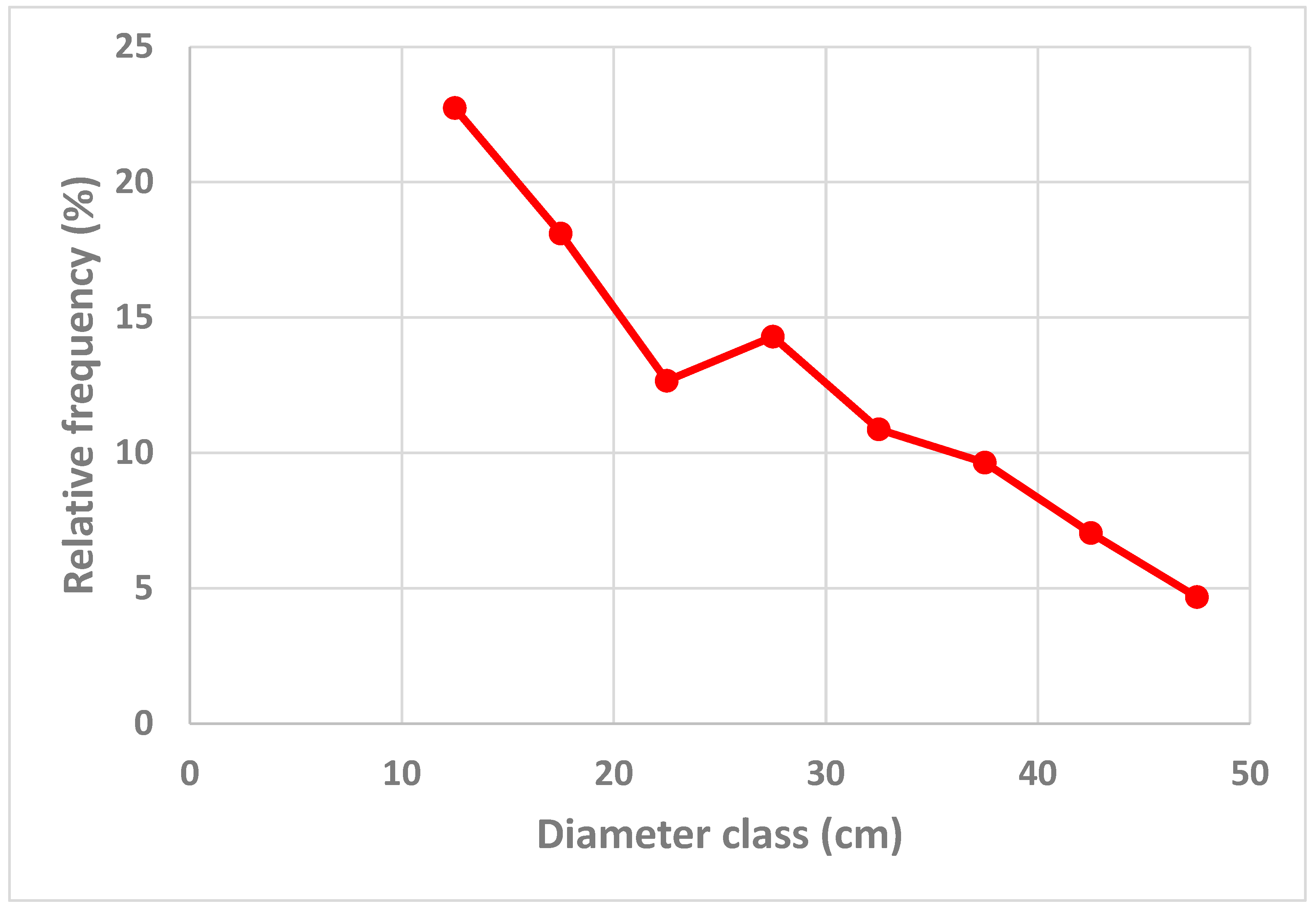
Figure 2.
The relative frequencies of trees in different diameter classes, according to the empirical data, found in Figure 1, and the predicted data, determined by the optimization model in the Appendix A.
Figure 2.
The relative frequencies of trees in different diameter classes, according to the empirical data, found in Figure 1, and the predicted data, determined by the optimization model in the Appendix A.
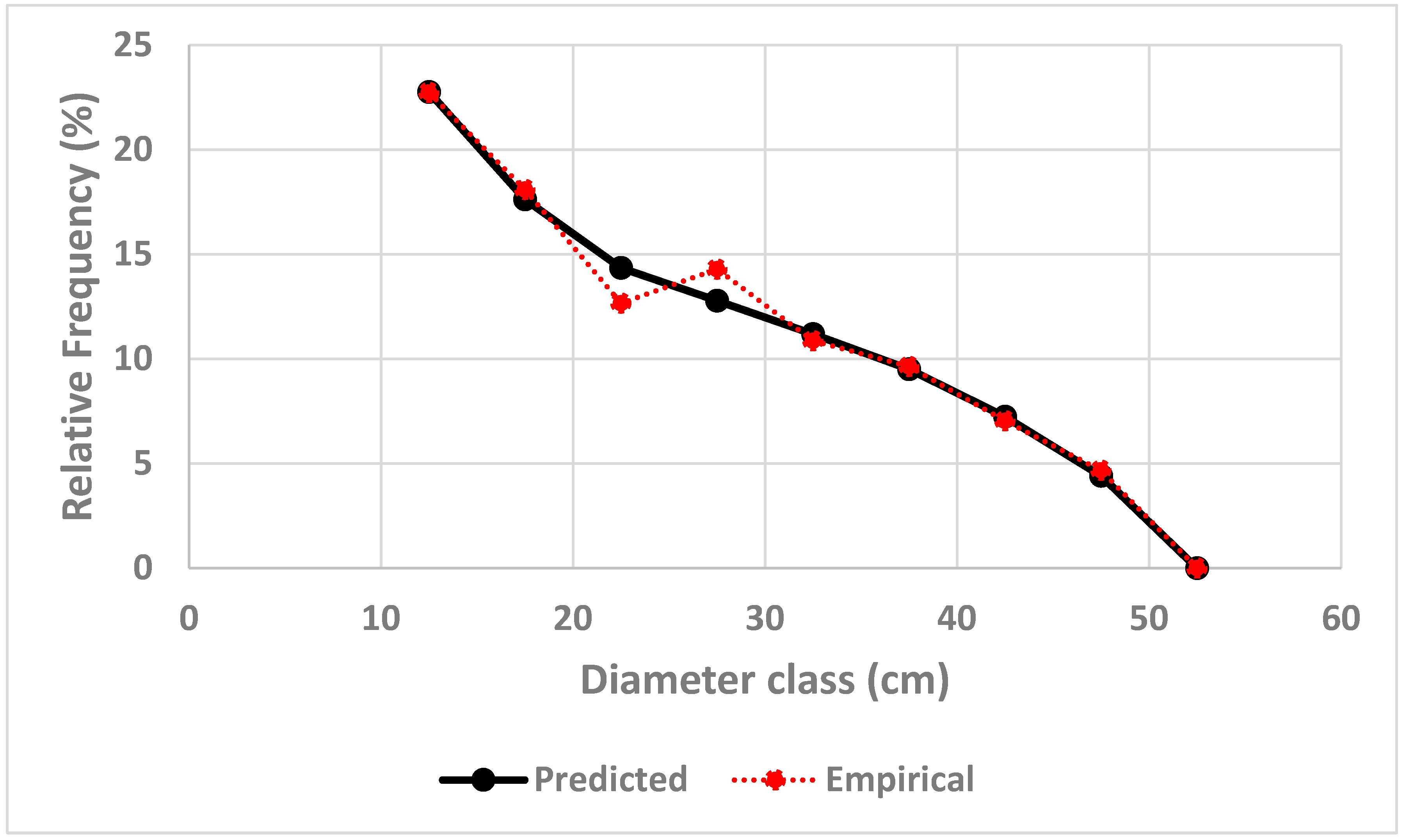
Figure 3.
Relative harvest, , determined by the optimization model.
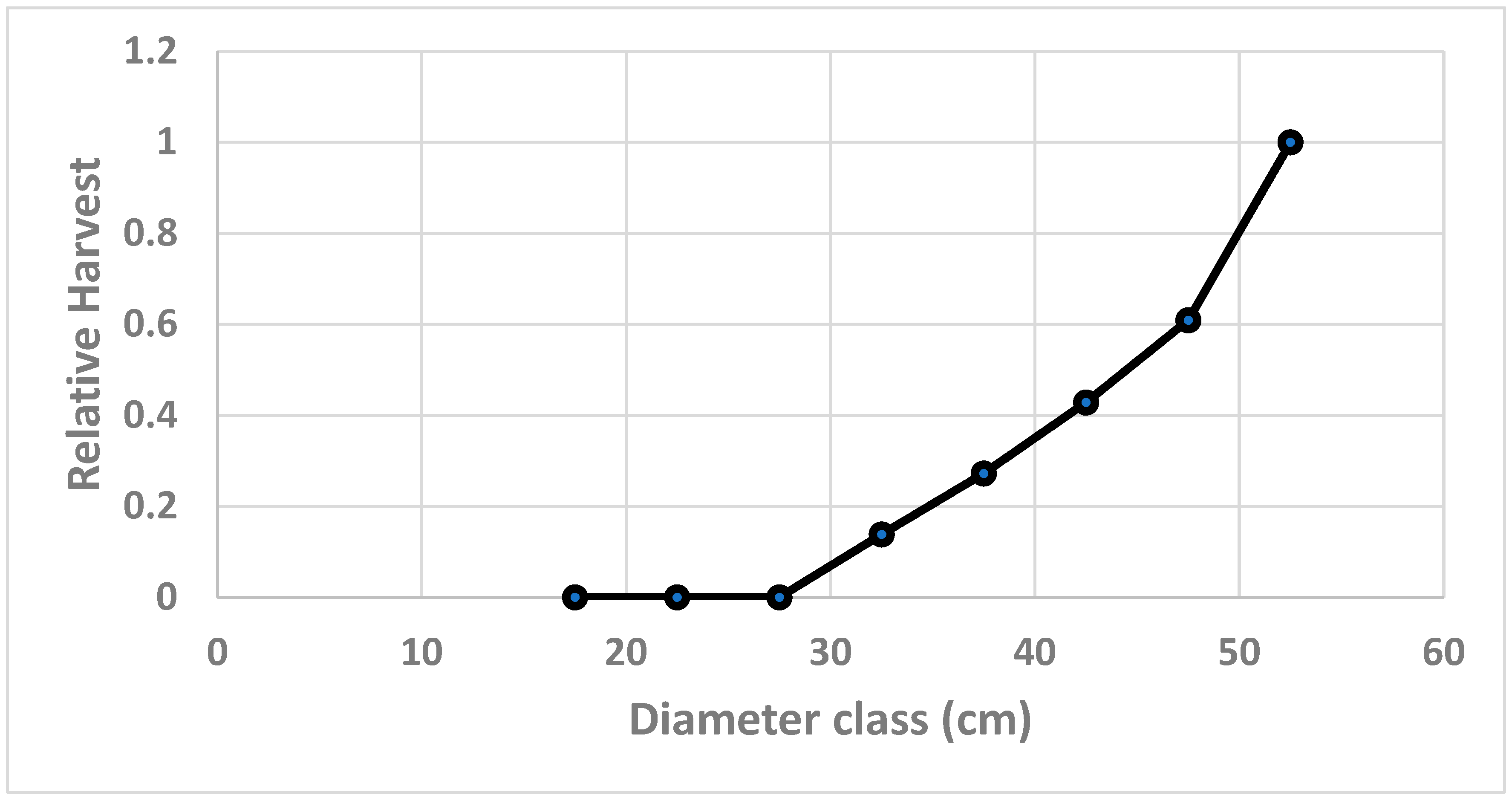
Figure 4.
Basal area the trees in a diameter class, m2 per hectare, determined by the optimization model. The classes as represented by the mean diameters of the corresponding 5 cm diameter classes.
Figure 4.
Basal area the trees in a diameter class, m2 per hectare, determined by the optimization model. The classes as represented by the mean diameters of the corresponding 5 cm diameter classes.
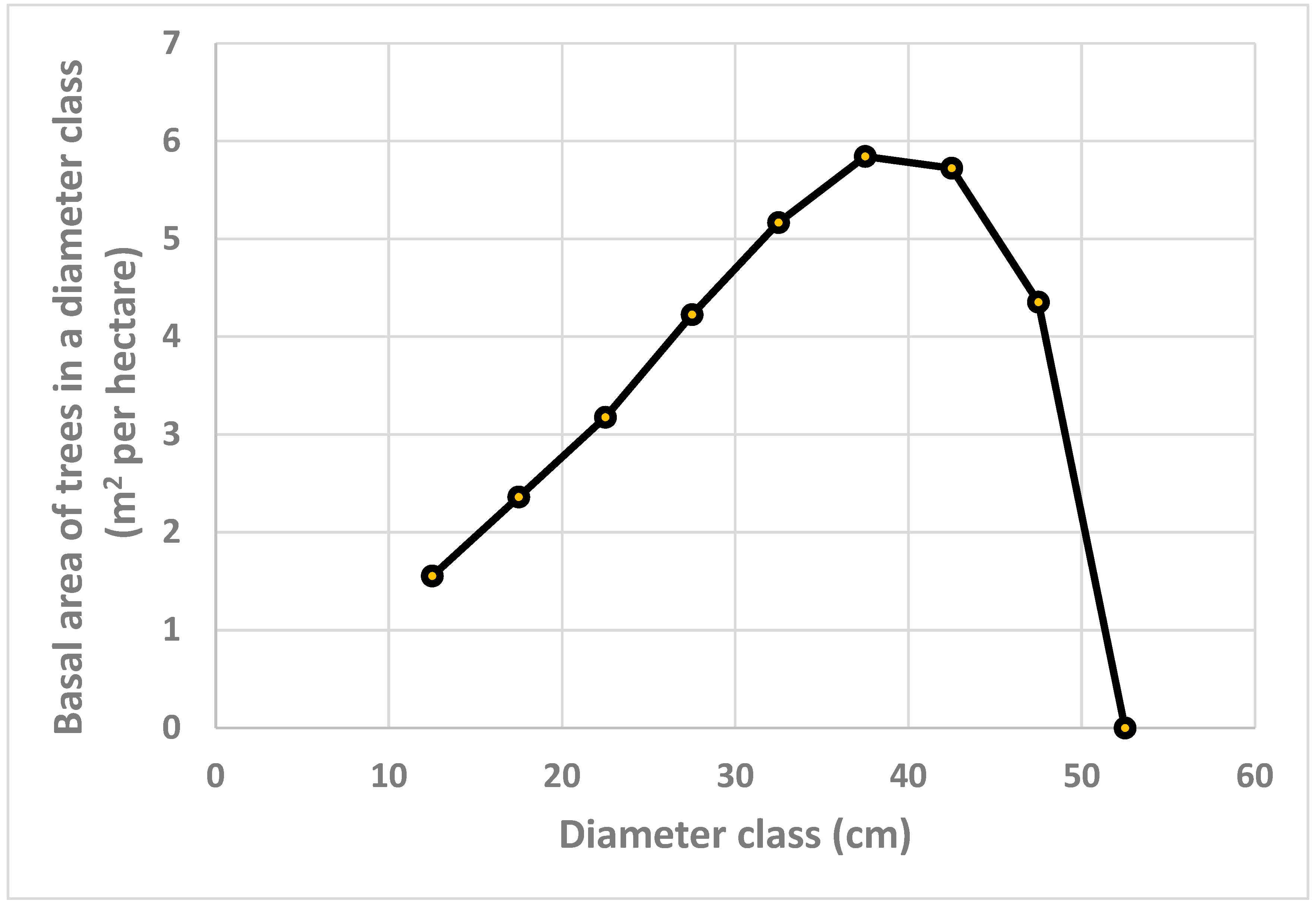
Figure 5.
Basal area of larger trees, m2 per hectare, determined by the optimization model.
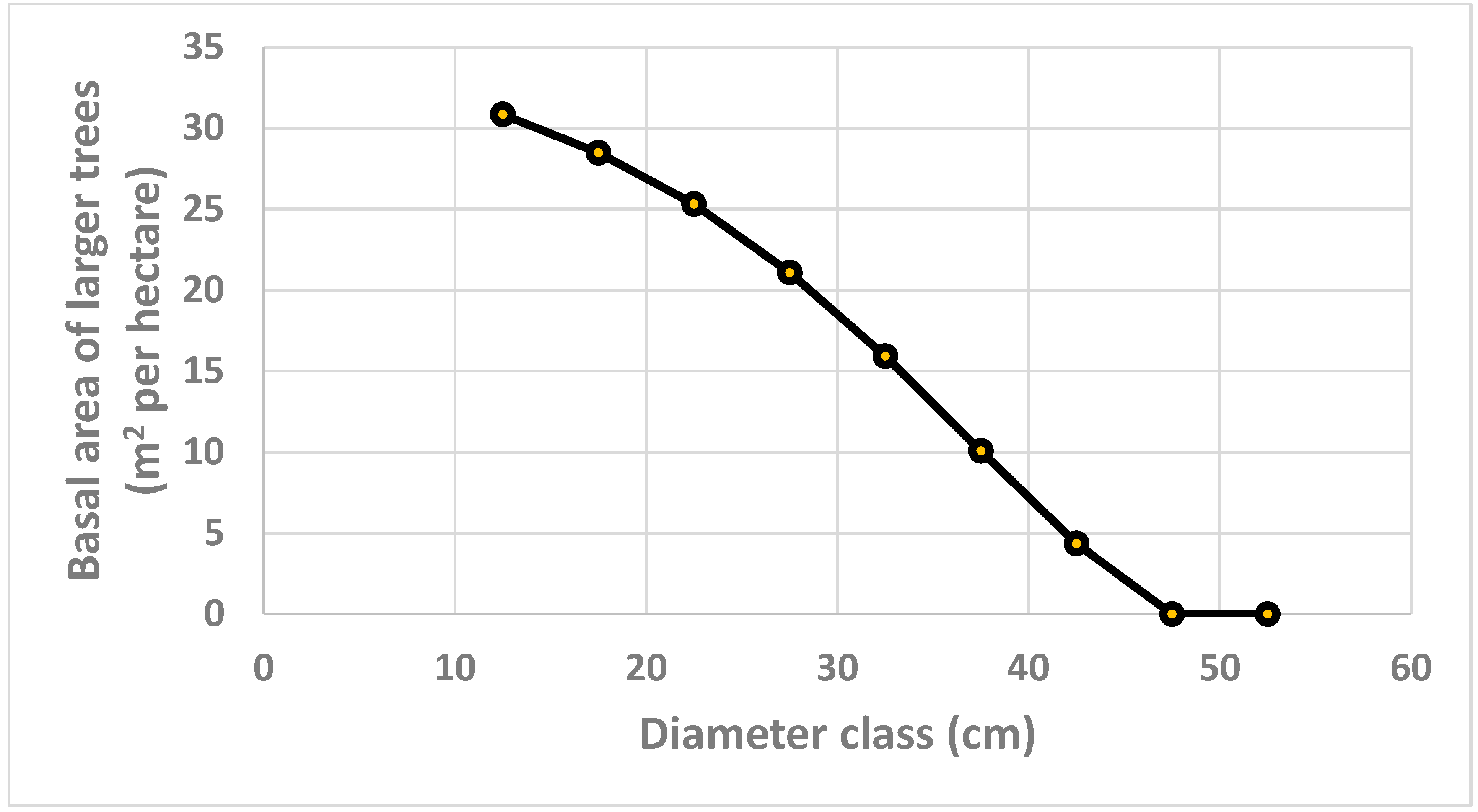
Figure 6.
Equilibrium number of stems per hectare, in different diameter classes, determined by the optimization model.
Figure 6.
Equilibrium number of stems per hectare, in different diameter classes, determined by the optimization model.
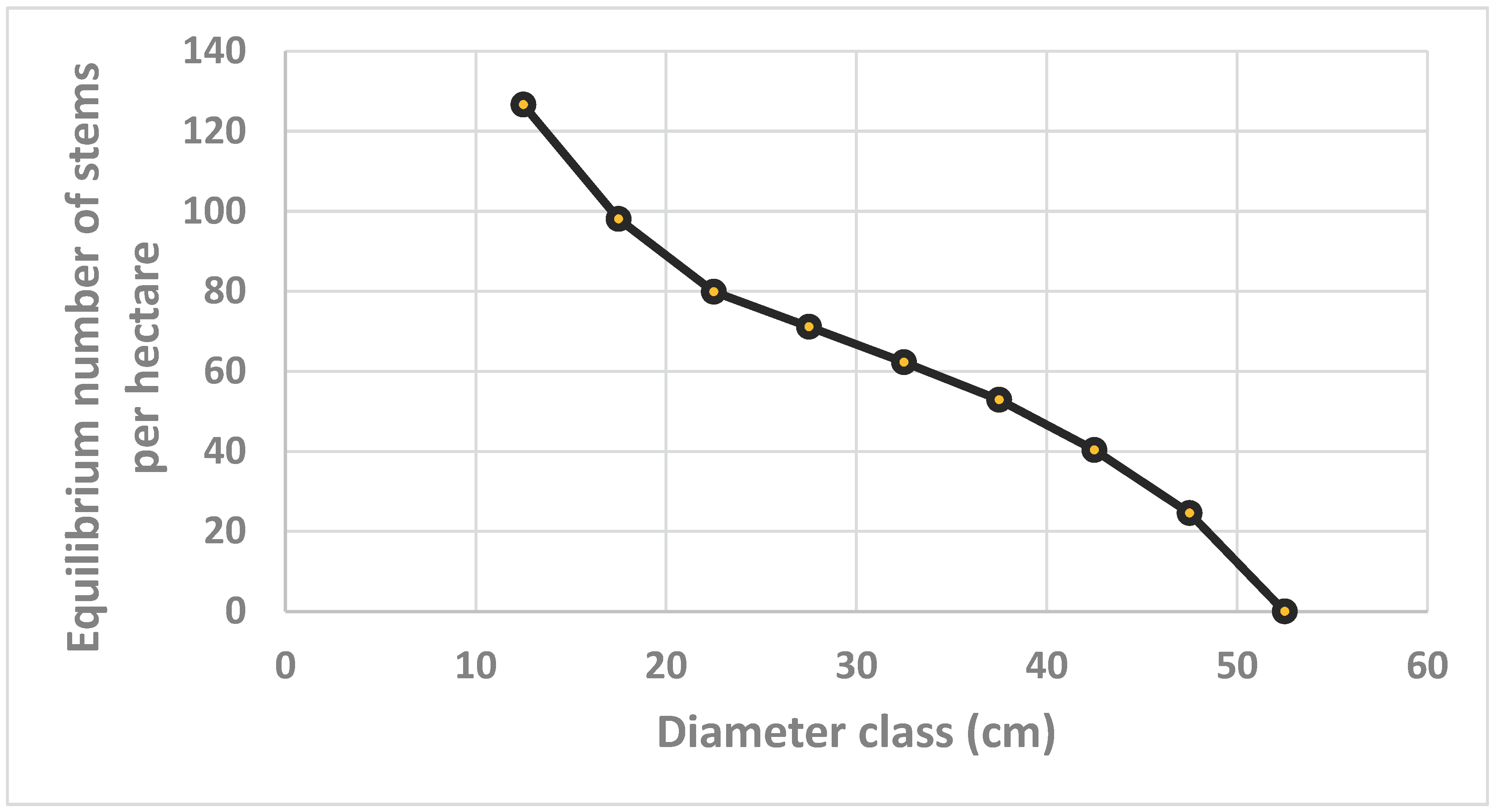

Table 1.
Derived general statistical results. Detailed descriptions are found in the Appendix A.
Table 1.
Derived general statistical results. Detailed descriptions are found in the Appendix A.
| Variable | Notation | Estimate |
|---|---|---|
| Total sum of squares | SSTOT | 241.216 |
| Residual sum of squares | SSRES | 5.599311 |
| Multiple regression coefficient | R2 | 0.9767872 |
| Variance of the residuals | VAR_RES | 0.7999016 |
| Standard deviation of the residuals | STDEV_RES | 0.8943722 |
Table 2.
Optimized parameter estimates.
| Analytical notation | Numerical notation | Estimate | Parameter reference: |
|---|---|---|---|
| HPAR | 0.2468048 | Equation (38) & Appendix A | |
| DPAR | -0.0177103 | Equation (42) & Appendix A | |
| GPAR | -6.17579E-07 | Equation (42) & Appendix A | |
| BAL_EXP | 4 | Equation (42) & Appendix A | |
| LPAR | 0.2275699 | Appendix A |
Disclaimer/Publisher’s Note: The statements, opinions and data contained in all publications are solely those of the individual author(s) and contributor(s) and not of MDPI and/or the editor(s). MDPI and/or the editor(s) disclaim responsibility for any injury to people or property resulting from any ideas, methods, instructions or products referred to in the content. |
© 2024 by the authors. Licensee MDPI, Basel, Switzerland. This article is an open access article distributed under the terms and conditions of the Creative Commons Attribution (CC BY) license (http://creativecommons.org/licenses/by/4.0/).
Copyright: This open access article is published under a Creative Commons CC BY 4.0 license, which permit the free download, distribution, and reuse, provided that the author and preprint are cited in any reuse.


