Submitted:
16 February 2024
Posted:
19 February 2024
You are already at the latest version
Abstract
Quantum logic is a well-structured theory, which has recently received some attention because of its fundamental relation to quantum computing. However, the complex foundation of quantum logic borrowing concepts from different branches of mathematics as well as its peculiar settings have made it a non-trivial task to device suitable applications. This article aims to propose for the first time an approach to use quantum logic in image processing at hand of a process for shape classification. We show how to make use of the principal component analysis to realize quantum logical propositions. In this way we are able to assign a concrete meaning to the rather abstract quantum logical concepts, and we are able to compute a probability measure from the principal components. For shape classification we consider encrypting given point clouds of different objects by making use of specific distance histograms. This enables to initiate the principal component analysis. At hand of experiments, we explore the possibility to distinguish between different geometrical objects and discuss the results in terms of quantum logical interpretation.
Keywords:
quantum logic
; principal component analysis
; shape classification
; Hilbert space
1. Introduction
Quantum logic [1,2,3] was developed as an approach to understand the structures of quantum physics at hand of a logical system. The starting point for this was above all the formulation of the Schrödinger equation and Heisenberg’s uncertainty principle. The latter in particular led to the conclusion that an uncertainty principle violates the distributive law in a logic-based framework. Over the last 70 years, various attempts that allow to incorporate the uncertainty principle into logic have been developed from this, with the pioneers being Birkhoff and von Neumann, Reichenbach and Mittelstaedt. In addition to the explanation of quantum mechanical phenomena, other areas of application for quantum logic have also emerged. The largest of these is quantum computing, where the underlying logic is featured in so-called quantum gates, see for example [4]. Other potential fields of applications have also been proposed, such as the evaluation of large datasets using contingency tables [5] or for quantum-inspired cognitive agents [6,7,8]. However, arguably because of the complex theoretical foundation of quantum logic and the peculiar settings described by it, up to now the range of applications has been limited.
The aim of this paper is to present a first approach to use quantum logic for shape classification. To our best knowledge, this article represents thereby the first attempt to make use of a quantum logical framework in image analysis.
In this paper, we want to base ourselves on the probably most popular interpretation of quantum logic by Birkhoff and von Neumann [1]. This in turn is based on the mathematical structures within quantum mechanics, namely Hilbert spaces and the associated operators. To do so leads us to the use of an orthomodular logic, which is a generalization of Boolean logic. Together, these form a projective geometry, which is one of the most important tools of quantum logic.
As an important computational component within our approach, we make use of the principal component analysis (PCA). The PCA method was proposed by Karl Pearson in the year 1901 [9]. Later in 1933, Harold Hotelling developed independently of Pearson an analogous method [10]. An overview on this method can be found in the book by Jolliffe [11]. The PCA is a statistical method to decouple meaningful information from high-dimensional data, reducing at the same time its dimensionality. This method is a powerful tool and is widely used in various fields including machine learning [12,13], image processing [14,15], genetics [16,17], and finance [18,19]. As we discuss in detail in this article, the mechanism of dimension reduction in PCA appears to be a natural fit to quantum logic. It is one of the contributions in this work to explore this connection.
Turning to computational ways to implement quantum logic, this paper represents in several ways a significant extension of an idea sketched by Wirsching [20]. In his work, he introduced a concept inspired by quantum logic that assigns to an incoming signal a similarity measure, making use of the Gram-Schmidt method. Our novel contributions may be described as follows. We illuminate in detail the connection between quantum logic to the possible building blocks of an application oriented framework. By doing this, we clarify in detail which properties of technical components are demanded for potential future applications. We consider a concrete application in the form of shape classification, which allows us to assign a concrete meaning to the rather abstract quantum logical concepts. As a technical difference to [20] we employ the PCA instead of the Gram-Schmidt method, which allows a more natural explanation of a probability measure in accordance to quantum logic. The PCA also allows a much stronger interpretation of computed results.
The paper is structured in two main parts. The first part, is presenting our model. Here we introduce the three important concepts for our paper. We will provide insides to quantum logic, the principal component analysis and how to connect these two topics with each other. With these concepts, we are able to apply quantum logic for a shape classification framework. The second part, of this paper, showcases our experiments. Where we start to explain how we preprocess our data, so it fulfils all needed properties derived from the theory part of this paper. Additionally, we want to verify our approach, by presenting some experiments. And finally, we end this paper with the conclusions and possible future work.
2. Description of Our Model
This section is dedicated to introducing all necessary details for the use of quantum logic for shape classification. First, we explain the concepts and operations in quantum logic. After that, we build the bridge from quantum logic towards the application in shape classification. Then we briefly recall the principal component analysis, and we show how to construct a probability measure based on these concepts.
2.1. Quantum Logic
We begin by introducing the fundamental framework of quantum logic, which is in close relation to the algebraic foundations of complete lattices. It was developed as an algebraic tool to provide an axiomatic construct for quantum mechanics where conventional approaches failed. The resulting axioms became known primarily through Birkhoff and von Neumann [1] and Piron [2] with his Geneva school’s approach [21].
2.1.1. Fundamental Lattice Setting of Quantum Logic
The idea of quantum logic is to operate on a quantum mechanical system in the form of a special lattice, which we will introduce now step by step for the readers’ convenience. We begin with the orthocomplemented lattice , where represent the minimal and maximal element, respectively, ∧ is the conjunction or meet, ∨ the disjunction or join, the orthocomplement and ≤ a partial order.
The orthocomplement is defined by the following three properties with the elements or propositions :
This quantum mechanical system contains a set of possible states, e.g. the elements of , . These states contain the set of all properties that are relevant for a particular realization of the system. In the quantum mechanical setting, if one considers a physical system that consists of multiple subsystems, quantum physics allows certain mixed states, namely entangled states, which make the difference between quantum theory and alternative classical models.
2.1.2. Reasoning behind the Projective Geometry of Quantum Logic
By the combination of Equation (1a) - (3b), we may arrive at Piron’s result, see [2], that the propositions from are in a one-to-one relation with the closed linear subspaces of a Hermitian vector space or pre-Hilbert space. Let us note that this result will be crucial to construct a computational approach relying on quantum logic.
In accordance to Piron’s result, the mentioned Hermitian vector space or pre-Hilbert space has a non-degenerating Hermitian form which allows the formation of the orthocomplementation of any subset S in the sense of an orthogonality relation concerning the Hermitian form. Here, a subset is described as closed if the involution law (1b) applies.
At this point, we will briefly summarize how the lattice operations affect the subspaces of the Hilbert space according to Birkhoff and von Neumann [1]:
-
where the + represents the vector sum, such that the join or union of two subspaces is the smallest subspace encompassing both these subspaces,
- is the orthogonal complement of , such that for all and , and , where is the singleton that only consists of the null vector,
- is equal to for all .
The lattice of subspaces of a Hermitian vector space with the orthogonal complement operation is in general not distributive, i.e. . As an example for this statement, we consider the lattice of the subspaces of , which consists of the two-dimensional elements of , with the component-wise addition
and component-wise multiplication
To make it clear that we are talking about subspaces here, we write the ordered pairs in notation. The following then applies:
and at the same time
holds true. This is a contradiction to distributivity.
The non-distributivity is probably the best-known property of quantum logic. A classical physical example of this is Heisenberg’s uncertainty principle, according to which it is not possible to determine the position and the momentum at the same time, as the measurement influences the system. To be precisely, let there be three propositions , which correspond to a momentum measurement a and a position measurement that is divided in a left interval b and a right interval c. Then, according to Heisenberg’s uncertainty principle, the terms and could produce different results, since in the second term we have always a momentum and a position measurement at the same time. Therefore, this represents another contradiction to distributivity.
For this reason, a weakened form of distributivity is used in the form of
Especially, there is a connection between the orthomodularity and the Hilbert space, which was proven by Solér [22] and states that the pre-Hilbert space is complete if and only if the propositions satisfy the orthomodular law (4). Because of this orthomodularity property, we will use so-called orthomodular lattices in the following. This leads to the main result that Birkhoff and von Neumann [1] as well as Piron [2] have proven, in the form of the aforementioned connection of the lattice and the Hilbert space.
2.1.3. Projective Geometry of Quantum Logic
After having introduced some basic algebraic concepts of quantum logic, we will introduce the axiomatic theory presented by von Neumann for the remainder of this section, leading to the foundation of a projective geometry. Our exposition of this is based on the book by Chiara et al. [3].
As for a beginning, let us point out that the quantum logical states have associated state vectors in terms of wave functions that form in general an infinite-dimensional complex Hilbert space . The wave functions are the reason the corresponding Hilbert space is called phase space. Thereby, a distinction is made between the pure states already mentioned, which are unit vectors of the Hilbert space, and mixed states, which are represented by density operators of the Hilbert space. However, it has already been shown that this can be realized with (not necessarily complex) finite-dimensional spaces of at least rank four, see for example [2]. This means for the case that the elements of are the vector subspaces of .
In the following, we will replace with the set of closed subspaces of . Each pure state or unit vector enables a projection , which is the projection onto the one-dimensional closed subspace corresponding to . However, as for the mixed states, it should be noted that not every possible density operator can be represented by a projection .
The mentioned one-to-one connection by Piron’s result, between the state space and the phase space, relies on the fact that one can map one-dimensional subspaces of the Hilbert space into one point (atom) and the linear subspaces of the Hilbert space onto linear sets, i.e. straight lines through at least two points. Consequently, we have a one-to-one correspondence between the set of all projection operators and the set of closed subspaces of . This leads to a projection from the phase space into the state space, since the projective space consists of the states of the system. The resulting projective geometry is the main reason why quantum logic is used in general.
2.1.4. Construction of the Projection Operators and the Probability Measure
The aforementioned Hilbert space formalism allows us to use corresponding multidimensional models and assign probabilities to them. For this purpose, we consider the variables , , which take on one of the finitely many values , , in a measurement that defines the state of the system. Thereby, will be called observables and the output of the measurement of an observable leads to an event E, which we will interpret as a projection.
As for the relation between a physical measurement and its mathematical realization, this means that every measurement will be represented by a self-adjoint operator on the Hilbert space, which one refers to as observable. The eigenvectors of such an operator form an orthonormal basis for the Hilbert space, and each possible result of this measurement corresponds to one of the vectors that form the basis. The individual events are subspaces of the Hilbert space, and we associate each subspace (or the corresponding event E) with a projector , which projects vectors into the corresponding subspace and fulfils , where represents the Hermitian transpose of .
This projector allows us to assign an expected value to an observable, i.e. that the observable is in a state, which is represented by the pure state . That means, if is any unit vector, we can define a probability measure as
For practical applications of quantum logic, it appears to be essential to create appropriate projectors. So far we have only indicated some properties that they must fulfil, but not how to construct one. We will now do this as a first step for projectors on pure states. If we explain the projection operator on the one-dimensional subspace belonging to the pure state as for all , we obtain the notation
where , and Tr is the trace functional, which is more common in quantum mechanics. This means will have value 1 in the state or in other words we have the certain verification of an event that belongs to an arbitrarily closed subspace E by a pure state iff is an element of :
This representation can also be extended to mixed states. To do this, we consider a mixed state as a superposition of several pure states and can thus explain the density operator mentioned above as
This allows us to specify the corresponding probability measure as a convex combination:
which is the usual way of representing the probability that the system is in a mixed state and fulfils an event E by the projection according to the Born rule. In particular, Gleason [23] showed that this representation is the only one that allows probabilities to be assigned to a subspace in the sense of a positive measure for dimensions greater than two.
2.2. Towards Application of Quantum Logic for Shape Classification
So far, we have looked at the basic properties and some conclusions in quantum logic. Now we want to put these into the connection to an application and show how to make use of quantum logic in a shape classification framework as exemplified.
To make this connection more precise, we explain L in a symbolic sense as the collection of all properties of our system , or in other words as a collection of "yes" or "no" experiments. A distinction is not necessary in this sense, since each property can be queried with a yes or no question and vice versa. If we transfer this to a quantum system, L corresponds to the collection of all closed subspaces of our Hilbert space , and we say that such an experiment is "true" if the state vector lies in the corresponding closed subspace E of . In this case, we say "E is true" and we only deny it with certainty if the state vector lies in .
2.2.1. Quantum Logical Meaning of a Shape
By transferring this idea to shapes, we may understand a state vector as a vector that contains certain predetermined information about the shapes under consideration. Since our goal is to decide whether a given shape S corresponds to a certain shape class or not, we can also identify this question as a "yes" or "no" question.
Consequently, we would answer "yes" if the shape under consideration S corresponds to a specific shape class, if the corresponding state vector lies in a closed subspace of the Hilbert space. This closed subspace would then have to be associated with this specific shape class in this sense.
2.2.2. Idea behind Shape Classification with Quantum Logic
In this context, the quantum logical setting offers the advantage that we can not only say whether a shape S belongs to a certain class or not, but even with what probability. In this sense, it should be noted that S could have any shape regardless of the experiment we conduct. However, if it is a type of shape that we have used to span the Hilbert space, then S would correspond to a pure state, and we could use the equation (5). Otherwise, if S would be a superposition of the types of shapes we used to construct , we would use equation (9). At this point, it should also be emphasized that when we talk about the Hilbert space spanned by these types of shapes, we mean a subspace of the Hilbert space of all possible shapes, which is itself a Hilbert space in order to apply quantum logic to it.
2.2.3. Necessary Considerations for Shape Classification
If we follow this train of thought further, the underlying projection operator would have to map a vector onto a one-dimensional subspace belonging to the type of geometric shape under consideration. This means that we need a separate operator for each type of shape, i.e. triangles, squares, etc., with which we can decide to what extent the state vector under consideration corresponds to this type of shape.
In order to express the shape classification task quantum logically, we therefore need a Hilbert space of shapes on which we can work. We have to span this space with axes that we associate with certain types of shapes and in order to obtain a probability for the classification we have to compare the considered shape S with the representatives of these axes.
To do this, we first have to convert all shapes into normalized vectors of the same length, which contain enough information about these spans to make meaningful decisions. We will divide these vectors into directions, that have the greatest influence, which we realize here by using the principal component analysis. These should then be the directions that contribute significantly to categorizing a shape as a triangle, for example. We therefore use them to construct our projection operators. We will devote the rest of this section to realizing this prepared setting.
2.3. Summary of Principal Component Analysis (PCA)
The PCA is a statistical technique to reduce the dimension of a large dataset while preserving most of the contained information. It maps a large sized dataset into a smaller number of new variables called principal components.
The first principal component belongs to the direction where the dataset has the highest variance and the second principal component belongs to the direction with the second-highest variance, and so on. All directions produced this way are orthogonal to each other, or in terms of quantum mechanics, they are uncorrelated.
Let us recall the PCA method step-by-step. Assume a given dataset consisting of random vectors of length k. The r random vectors will be merged into a matrix
The first step in the PCA method is to centre the data. Therefore, we calculate the mean value for each row of and get the mean value vector . After that, we can subtract from each random vector X in . We will write the subtraction like: .
Second, we compute the covariance matrix via
As a third step, we calculate the spectral decomposition of the matrix :
Where is the matrix of the sorted eigenvalues. The matrix contains the normalized eigenvectors with of belonging to eigenvalue , denote the corresponding eigenspace. The vectors will act as the directions mentioned in at the beginning of this section.
The fourth and last step will be the calculation of the principal components Y of an already centred random vector X
with the ith principal component, the ith unit vector and the dot product in a Hilbert space.
A useful property of the principal components is that the variance of the ith component will be the ith eigenvalue,
This will ensure that the first principal component has the largest variation since the eigenvalues are ordered. One may interpret the ith principal component as the share of X on the direction .
2.4. Classification by Quantum Logic
In this section, we want to build the bridge between the probability measure of the quantum logic and the principal components from the previous section. Before we can connect these two components, we want to expand the notation of the principal components.
2.4.1. Expanding the Notation
Consider a set of geometrical objects O with the index set G. The set O consists of the geometrical shape classes , , and will be used to store the various classes we want to classify. In this context, refers to two different shape classes if and refers to the same shape class if .
By using only random vectors of shape class with for the PCA formalism, we obtain the eigenspace and mean vector for this specific shape class.
In Figure 1 we illustrate the obtained eigenspaces for a triangle and square. We make use of the geometrical object sets with containing only triangles and squares. In this sense, is the eigenspace of the triangle and belongs to the square shape class. Analogously, we depict the mean vector .
We will adapt the notation even further. In Equation (13) we want to make sure that we can distinguish between the shape class that provides a random vector and the eigenspace of another shape class , for . This will enhance the notation of the principal component vector.
As an example, will describe the principal components obtained from a random vector from the triangle shape class and the square shape class eigenspace .
2.4.2. Probability Measure Constructed by Quantum Logic
The theory of the quantum logic, especially, Equation (5) will build the foundation of the presented classification approach. This formula allows us to construct a probability measure for any unit vector and projection operator .
In our setting, the random vector X of an arbitrary shape class acts as the unit vector . In Section 2.2, we introduced a projection operator for pure states and a density operator for mixed states that consists of pure states. The eigenvectors , from the PCA, will take the role of the pure states. Hence, we need to show that a projection operator obtained from the eigenvectors, fulfils the conditions ( is Hermitian and idempotent) presented in Section 2.1 for a suitable projection operator.
We construct the operator via
The resulting matrix is symmetric and real-valued, i.e. the condition is fulfilled for this operator. To prove the idempotence, we calculate
As such, our fulfils all the requirements of a projection operator, and we can now use it to calculate a probability measure for a pure state, or normalized random vector, X.
This formula allows us to compute the probability measure via the principal components. And therefore, we are able to check if a normalized random vector X belongs to a certain shape class with , by computing the principal components according to (15).
Since the maximal dimension of our constructed Hilbert space is k, we will face some issues, that we want to address now. As a recall of Equation (7), setting , will result in a probability measure of one, since we make use of all principal components. Like we mentioned at the end of Section 2.3, we can interpret the principal component as the share of X onto the direction . Using would lead to the fact, that we make use of k orthogonal directions in a k-dimensional Hilbert space. Hence, the eigenvectors will span the complete space, regardlessly of the considered shape class. Computing the probability measure of a random vector X belonging to shape class with will lead to a value of one. To avoid this issue, we change the condition to .
In Figure 1 we visualize this issue. There we have a two-dimensional space with two results from the PCA, namely the eigenvector spaces from a triangle and a square shape class, respectively.
Considering the projection of the now normalized random vector X onto the first eigenvectors of the triangle and square, we can argue that the probability that X will be labelled as a member of the square shape class is much higher than the probability to be labelled as a triangle. Since, the share of X onto is bigger than the share onto .
If we used both eigenvectors for each shape and compute the probability measure, we would get one for both shapes classes, since each eigenvector pair is a suitable description of the two-dimensional plane and therefore the vector X is fully described by both pairs.
In the end, we will rewrite Equation (17) to be fit for the classification and take into account these remarks:
We finally expect that our approach will lead to relatively high probability measures for the case in . Since the first principal components should have greater values, than the case for .
2.4.3. Quantum Logical Interpretation
A quantum logical interpretation of the combination would be, that each of the eigenvectors produced from the PCA will represent an assertion about a specific shape class. We will not know, the exact wording of these assertions, but we know two things.
The first thing is, that the initial assertion should be the most controversial, since the principal component vary the most, see (14). Adding more assertions, i.e. increasing , will lead to more and more specific perception of a shape. As the variation of the last assertion is small or negligible, we can safely disregard it.
Second, using all possible assertions, we should be able to confidently tell, if a random vector X belongs to a specific shape class or not. And, with (18) we are also able to put a percentage value on this "belonging".
3. The Experiment and the Preparation
We would like to point out again, that one of the contributions of this paper is the exposition of the connection between PCA and quantum logic. In this section, we will dedicate ourselves to have a closer look at a possible way to convert our data into a format that can utilize this connection.
To be more precise, we will now explain our data format and then move on to illustrate the preprocessing to generate the random vectors X from our shape dataset. Then, we will discuss a way of shape classification and provide an algorithmic pipeline. Last but not least, we will show and discuss the produced results.
3.1. Shape Data
For the start, we want to briefly explain the concept of a shape as we employ it. A shape S is considered to be realized by a closed curve in a 2-dimensional space, . Such a curve itself, is established as a point cloud with points for . The x and y coordinates of a single point are denoted via and . In this way, the point cloud P will represent a discrete realization of the shape S.
3.1.1. The Dataset
The core of the used dataset is the geometric shape dataset [25]. This dataset consists of 10,000 pictures per shape and contains pictures of triangles, squares, pentagons, hexagons, heptagons, octagons, nonagons, circles, and stars (with a centred pentagonal hole) in different rotations, sizes, positions, and colours of the shapes themselves and the background. We also used this dataset in a previous paper, see [24]. There we already transformed the images into point clouds. These point clouds define the starting point for our preprocessing.
The process we employ to boil down a colour image to a point cloud is sketched in Figure 2, and will be shortly reviewed now. First, we select one colour channel of the image and obtain a grey scaled version of the image. The second step is the transformation into a binary black-and-white image. After that, we use the bwboundaries MATLAB routine to compute the point clouds.
The reason behind using only one colour channel of the image to create a greyscale image is that the pictures from the dataset were originally created to have a constant mean value over the whole image. Doing otherwise, we would end up with no difference between background and shape in the image, and we would not be able to produce a binary image for further processing.
For the stars, the MATLAB routine bwboundaries produced two to three point clouds, i.e. one point cloud of the star, one pentagon point cloud and sometimes an image border point cloud. And these point clouds swapped their order from image to image. In the end, we were not able to automatically select only the useful point cloud. Since the proceeding is troublesome when producing point clouds from the star images, we chose to ignore these data and consider only the remaining geometrical shapes of the given dataset.
With the remaining dataset we have a geometrical shape set
where we denoted the different shapes with their number of vertices. For the circle, we decided to use here the symbol ∞ to encode the number of vertices.
The point clouds P that result from this process are ordered. Therefore, the point is the predecessor of the point in the images and in the dataset. Since the geometric shapes have different sizes in the images, the number of points per point cloud differs for different realizations of a shape class. So, we end up with point clouds with a size ranging from close to 100 to about 500.
3.2. Preprocessing
The point clouds are the starting point for the preprocessing that produces the random vectors X. Thus, the aim of the preprocessing is to convert all point clouds into normalized vectors of the same length, which are supposed to store enough information to make meaningful classifications possible.
3.2.1. Shape Descriptors and Signature
We will start to convert the point clouds P with their set of two-dimensional coordinates into a one-dimensional object.
This process should encrypt the geometry of the shapes in a meaningful and fast computable way. To this aim, we will adopt the D1 shape descriptors presented in [26].
This shape descriptor will calculate the distance between a point p from the point cloud P and a chosen centre point as
We make use of the Euclidean norm and the barycentre of the point cloud as the designated centre point . The centre point will thus be calculated by the arithmetic average of all n points of the point cloud. In Figure 3 we provide a visualization of this process for a triangle point cloud.
Now, we can create an ordered set of distance samples, also called ordered collection,
with a collection size of n, which corresponds to the number of points in the point cloud. The phrasing "ordered" refers to the fact that we will keep the intrinsic order of the points from the underlying point cloud P.
In Figure 4 we plotted the ordered samples of a triangle, pentagon, nonagon, and a circle. In these ordered samples, the vertices and the mid-edge points are recognizable through the higher and lower distance values. Additionally, we notice that the size of the shape impacts the produced distances d. This indicates that we still need some further preprocessing, which will be addressed by the next section.
3.2.2. Normalization
With the creation of the samples D, we eliminated dependencies on rotation and translation. The samples are still correlated to the size of our shape, like we already mentioned. For example, bigger shapes or image filling shapes will produce, on average, larger shape descriptors d since the distance between the centre point and the boundary points is larger, see Figure 4. The geometrical shapes of the triangle (first row) and nonagon (third row) are similar in size, and therefore the range of distance values is roughly similar. The pentagon (second row) and circle (fourth row) produces distances that vary around a value of 23 and 31.
Since we can have large and small shapes, we need to make the samples D more comparable with each other. A first approach to this problem is normalization. Since there are multiple ways of normalization, we want to present the used methods:
- Mean-Normalization
-
In order to ensure that all collections have the same mean value, we compute the mean value of a reference collection . The mean value for a collection will be calculated viaThe mean normalization of a collection D can then be calculated by
- Max-Normalization
- Similar to mean normalization, we will store the maximum of a reference collection . Then, we ensure that every collection D will have the same max value as the reference collection via
As for important implementation details, from the 10,000 samples per shape class, we simply take the first sample as the reference and normalize all other samples of that shape accordingly. The normalization is done per shape class; that is, triangles are normalized with respect to the reference triangle, squares with respect to the reference square, and so on.
3.2.3. Histogram Technique
After normalization, the samples are no longer dependent on the shape size. But still, the samples take into account the size of our point clouds. As the object size in the image increases, the number n of points in the point cloud P increases, and so does the number of elements in D. This is why we have different sample sizes up to now.
Another issue is that the single entries do not contain any real information, which may be crucial for the PCA. The first element in the sample is the normalized distance from the first point in the point cloud to the centre of the shape. This first point could be anywhere on the shape curve, as we have no control over the original sorting of the points, nor do we want to, as we do not want to limit the generalization properties of our approach unnecessarily.
To address these two points, we make use of a histogram technique. The length will be standardized into predetermined bins, providing an approximate representation of the distance distribution for each sample, denoted as D. Furthermore, we can store the results in the elements of a vector, and therefore even the position in a vector will encrypt information, which we consider as helpful for the usage with the PCA. We thus expect that the distribution of distances for a triangle compared to another triangle has more in common than the comparison to, e.g., a distribution of distances for a square.
Let us now briefly explain the idea behind the histograms and how to construct them in order to obtain a vector from a shape that meets our desired requirements. The main idea of a histogram, as we use it, is to distribute a sample over bins, where each bin represents a range of values, in our case the distances d from the samples D. Then, we can count how many elements fall into each of the bins. Therefore, it is crucial that the bins do not overlap, so that all values can only fall into one bin. In the end, we get a vector of length k, which stores the number of elements in each bin. And to keep the results comparable and to ensure that the entries store the same information, it is mandatory to use the same bins for all histograms of a single shape.
Since the sample size still differs from sample to sample, the bins of larger samples contain more elements than the bins of smaller samples. To solve this, we can normalize the histograms so that each histogram sums up to an area of one. And the area can be calculated as the sum over all products of the number of elements in a bin and the width of the bin. We make use of this approach, because most of the libraries used in programming have a density option for creating a histogram.
To summarize, with these histograms we have constructed a mathematical object in the form of a vector with meaningful axis entries from a shape that is independent of rotation, translation, and the size of the shape. In addition, the resulting vector has a defined length of , and each dimension of the vector has a relationship to a shape class that may differ from class to class. This means that we can use them as a starting point for the PCA analysis presented in Section 2.3.
3.3. Shape Classification
Our classification process is made up of two parts. The actual classification, where we determine the extent to which a shape belongs to a certain shape class, and the calculation of the hit rate to quantify the quality of our classification.
3.3.1. Classification Procedure
The core fundamentals for the classification are provided by Equation (18). If we have a normalized random vector X () from an unknown class, we compute the principal component vector obtained from the eigenvector spaces for . After that, we compute the probability for different of X using Equation (18). In the end, we need to choose the class, in which X has the highest probability.
Where we make use of the Euclidean norm for ‖·‖, and since the single term in the sum is made up by scalars, it simplifies to the square of the terms.
This procedure can be seen in Table 1, where we use the values from Figure 5 to support this method with numbers. In the image, we show the square of principal components (left) and (right) in percentage. We see that the square of the first component of contributes to the total probability and on the other hand the first component of will only contribute . So the outcome of Equation (24) would always be 3, since we got the highest probability measure for the projection operator of the triangle shape class, regardless of the chosen parameter .
3.3.2. Hit Rate
Consider, having multiple shape classes stored in O and each shape class for has random vectors X. We want to know how many vectors are classified to a specific shape class.
Generally speaking, we will call a classification successful if , and call it fail if for two shape classes and with . To quantify the quality of the classification, we introduce the hit rate , where we compute the quotient of the number of vectors of shape class classified as shape class over the total number of elements in class :
The hit rate will be visualized in a matrix styled plot, see Figure 6. The x-axis will represent the result of the classification, shape class , and the y-axis indicate the original shape class , for . The grey value in the entries of the hit rate matrix encode the value for the hit rate. A black entry will represent a value of one for , and for a value of zero, we will produce a white entry in the hit rate matrix.
3.4. The Experimental Pipeline
In this section, we want to present the pipelines and algorithms we used to create our results.
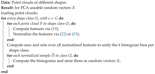
First, we need to preprocess the loaded point cloud as discussed, so that they can be used for the PCA. Algorithm 1 gives an overview of this process.
For all shape classes with , and for all point clouds belonging to class , we produce normalized samples. Then, we compute the max- and min-values of all normalized samples of each shape class to define the width of the bins. With these bins, we produce the histograms X from the samples . After this step, the preprocessing is finished.
| Algorithm 1: Algorithm for preprocessing the data. |
 |
The next step, would be the separation between the training data set and the test data set. We chose a ratio of 7:3. From the 10,000 histograms X in shape class , we use 7,000 for the PCA, and the remaining ones for training. The remaining 3,000 histograms will be used to test the matching quality of this approach.
In the third step, we produce with the PCA and the histograms labelled for training X the eigenspaces and mean values . The PCA is done separately for each shape class with . We store the produced eigenspaces and mean values for the classification process later on.
The fourth step, will calculate the classification via (15). This is illustrated in Algorithm 2. Here, we normalize the histograms labelled for testing again, so that . We will make use of the 2-norm for this, since in (18) refers to the induced norm from the inner product. In this case, it is the 2-norm, since we are using the Hilbert space . After that we compute the principal values for all combinations of using Equation (15).
| Algorithm 2: Compute the probability and construct the hit rate matrix. |
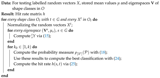 |
With , we can thus calculate probabilities via (18) and different . After that, we are able to produce a hit rate matrix using Equation (25).
Finally, we would like to emphasize the two main properties that the generated random vectors X should have: All vectors must have the same length, and each dimension should encrypt some information.
3.5. Experiments
For conducting the experiments, we would like to formulate two theses. First, we would like to see, that we are actual able to distinguish between different shape classes in O. Second, we would like to see, that this prediction gets better with an increasing value for .
For this aim, we will make use of the presented pipeline, and switching between the two normalizations, namely mean-Normalization and max-Normalization.
The resulting hit rate matrices for different and are depicted in Figure 7 and Figure 8. There, we increase row-wise from the top left image down to the bottom right image. Now, we will examine the hit rate matrices with respect to our two theses.
Both figures have a visible diagonal line, which is more dominant for shapes with higher number of nodes, i.e. hexagon up to circle. The mean-normalization tends to have more problems with low node shape classes than the max-normalization, because the diagonal line is faintly recognizable.
Concerning the second hypothesis, we notice that the diagonal gets more and more dominant if we increase the value of . It is remarkable that we achieve the best results for values of . However, we observe for an overall increase in the number of failed classifications. These failed attempts are more spread over multiple shape classes in the max-normalization and fixed to the hexagon shape class for the mean-normalization.
In Addition to the failed classifications, we notice other side effects and make an attempt to give an explanation for these.
We start with a potential explanation for the failed classifications. One reason could be in the inherent structure of the principal component calculation. There, we subtract the mean value of a specific shape class with from a random vector X. As a result, the random vector X belonging to the shape class should be closer to the origin of the eigenvector space spanned by this shape class than the random vectors of the other shape classes. Since points close to the origin are more sensitive to small errors, a small error could already change the share on different eigenvectors considerably, and therefore in the principal components, too. Random vectors of other shape classes may not have this problem, because their mean value differ from this sketched scenario. Therefore, random vectors of other shape classes, than the one used for testing, tend to stay away from the sensitive origin region. In consequence, these random vectors vary less in the principal components and may even be higher.
Another effect is, that with increasing values of the eigenvalues converge to zero. The latter used eigenvectors are therefore not meaningful enough. And so, these eigenvectors do not add much to the information describing the testing shape, but allow random vectors from other shapes to increase their probability measure. Ending up with the failed classifications in the bottom left images in the presented figures.
To summarize, on the one hand, we notice that an interpretable, meaningful classification is possible. Even with this relative simple approach, we are able to partially get correct classifications. Note that an advantage of such a simple approach is, for example, that it can be easily extended to 3D shape point clouds. On the other hand, we know that the presented preprocessing can be optimized in some aspects for better shape classification.
4. Conclusion and Future Work
In the first part of the article, we presented the main theoretical aspects. We illuminated the mathematical backbone of the quantum logic, principal component analyses (PCA) and the connection between these two topics. With the presented formalism, the reader should be able to swap the PCA method with some other method, which may be considered useful for a particular task. If such a method provides Hermitian and idempotent operators, respectively, any new method can be used for establishing a connection to quantum logic.
The presented theory is general enough to work with mixed states, e.g. with triangle-square hybrid shapes, but the formalism of the PCA inherently refers to pure states without putting in adjustments. One still has to find out, which may be a topic for future work, how to mix eigenvector spaces, e.g. of triangles and squares, to keep the general procedure to calculate probabilities via the eigenvector spaces.
The presented preprocessing may be optimized in future work for better results. In this paper, the main idea was to study a first approach to work in a meaningful task in image processing with the theoretical aspects of quantum logic. Especially, we think, that the classification results can be improved with a better preprocessing. The usage of the histograms, while at first glance adequate, seems to not preserve the inherent structure of the point clouds adequately enough. For example, one may have different point cloud distributions that could lead to the same histogram.
Another point for optimization is the described classification proceeding. We labelled a random vector to the shape class with the highest probability, and ended up in some cases with a failed classification. This process leaves open whether the correct shape class was close to or far from the final one. With this in mind, we think that a ranking of the classification results would be more useful than committing to one shape class.
A final point that we would like to discuss in the future for optimizing our approach is that we did not fully utilize the possibilities of the PCA formalism. The ordered eigenvalues allow us to reduce the eigenspaces to only necessary directions, and with the quantum logic we are also able to quantify the error by doing so. This reduction could thus be explored more consequently in our presented pipeline, which could lead to some better classification results.
Author Contributions
Conceptualization, A.K. and M.K.; methodology, A.K.; software, A.K.; validation, A.K., M.K. and M.B.; formal analysis, M.K. and A.K.; investigation, A.K.; resources, A.K., M.K. and M.B.; data curation, A.K.; writing—original draft preparation, A.K. and M.K.; writing—review and editing, A.K., M.K. and M.B.; visualization, A.K.; supervision, A.K., M.K. and M.B.; project administration, A.K., M.K. and M.B.; All authors have read and agreed to the published version of the manuscript.
Data Availability Statement
The dataset of all images can be found via [25]. The code is availeble at: https://github.com/koehlale/A_First_Approach_to_Quantum_Logical_Shape_Classification_Framework
References
- Birkhoff, G.; Von Neumann, J. The Logic of Quantum Mechanics. Annals of Mathematics 1936, 37, 823–843. [Google Scholar] [CrossRef]
- Piron, C. Axiomatique de la théorie quantique. Les rencontres physiciens-mathématiciens de Strasbourg -RCP25 1973, 16. [Google Scholar]
- Dalla Chiara, M.L.; Giuntini, R.; Greechie, R. Reasoning in quantum theory: sharp and unsharp quantum logics; Vol. 22, Springer Science & Business Media, 2013. [CrossRef]
- Rieffel, E.; Polak, W. An introduction to quantum computing for non-physicists. ACM Computing Surveys (CSUR) 2000, 32, 300–335. [Google Scholar] [CrossRef]
- Busemeyer, J.; Zheng, W. Data fusion using Hilbert space multi-dimensional models. Theoretical Computer Science 2018, 752, 41–55. [Google Scholar] [CrossRef]
- Huber-Liebl, M.; Römer, R.; Wirsching, G.; Schmitt, I.; Wolff, M.; others. Quantum-inspired Cognitive Agents, 2022. [CrossRef]
- Wolff, M.; Huber, M.; Wirsching, G.; Römer, R.; Graben, P.b.; Schmitt, I. Towards a Quantum Mechanical Model of the Inner Stage of Cognitive Agents. 2018 9th IEEE International Conference on Cognitive Infocommunications (CogInfoCom), 2018, pp. 147–152. [CrossRef]
- Schmitt, I.; Romer, R.; Wirsching, G.; Wolff, M. Denormalized quantum density operators for encoding semantic uncertainty in cognitive agents. 2017 8th IEEE International Conference on Cognitive Infocommunications (CogInfoCom), 2017, pp. 165–170. [CrossRef]
- Pearson, K. LIII. On lines and planes of closest fit to systems of points in space. Philosophical Magazine Series 1 1901, 2, 559–572. [CrossRef]
- Hotelling, H. Analysis of a complex of statistical variables into principal components. Journal of Educational Psychology 1933, 24, 417–441. [Google Scholar] [CrossRef]
- Jolliffe, I.T. Principal Component Analysis, 2 ed.; Springer Series in Statistics, Springer-Verlag, 2002. [CrossRef]
- Chen, J.; Jenkins, W.K. Facial recognition with PCA and machine learning methods. 2017 IEEE 60th International Midwest Symposium on Circuits and Systems (MWSCAS). IEEE, 2017. [CrossRef]
- Howley, T.; Madden, M.G.; O’Connell, M.L.; Ryder, A.G., The Effect of Principal Component Analysis on Machine Learning Accuracy with High Dimensional Spectral Data. In Applications and Innovations in Intelligent Systems XIII; Springer London, 2005; pp. 209–222. [CrossRef]
- Bouwmans, T.; Javed, S.; Zhang, H.; Lin, Z.; Otazo, R. On the Applications of Robust PCA in Image and Video Processing. Proceedings of the IEEE 2018, 106, 1427–1457. [Google Scholar] [CrossRef]
- Patil, U.; Mudengudi, U. Image fusion using hierarchical PCA. 2011 International Conference on Image Information Processing. IEEE, 2011. [CrossRef]
- Reich, D.; Price, A.L.; Patterson, N. Principal component analysis of genetic data. Nature Genetics 2008, 40, 491–492. [Google Scholar] [CrossRef] [PubMed]
- McVean, G. A Genealogical Interpretation of Principal Components Analysis. PLoS Genetics 2009, 5, e1000686. [Google Scholar] [CrossRef] [PubMed]
- Nobre, J.; Neves, R.F. Combining Principal Component Analysis, Discrete Wavelet Transform and XGBoost to trade in the financial markets. Expert Systems with Applications 2019, 125, 181–194. [Google Scholar] [CrossRef]
- Le, T.H.; Le, H.C.; Taghizadeh-Hesary, F. Does financial inclusion impact CO2 emissions? Evidence from Asia. Finance Research Letters 2020, 34, 101451. [Google Scholar] [CrossRef]
- Wirsching, G. Quantum-Inspired Uncertainty Quantification. Frontiers in Computer Science 2022, 3. [Google Scholar] [CrossRef]
- Stubbe, I. The Geneva School approach to the axiomatic foundations of physics, 1999.
- Soler, M.P. Characterization of Hilbert spaces by orthomodular spaces. Communications in Algebra 1995, 23, 219–243. [Google Scholar] [CrossRef]
- Gleason, A.M. Measures on the closed subspaces of a Hilbert space. In The Logico-Algebraic Approach to Quantum Mechanics; Springer, 1975; pp. 123–133. [CrossRef]
- Köhler, A.; Rigi, A.; Breuss, M. Fast Shape Classification Using Kolmogorov-Smirnov Statistics. Computer Science Research Notes 2022, 3201, 172–180. [Google Scholar] [CrossRef]
- Korchi, A.E. 2D geometric shapes dataset. Mendeley Data, 2020. V1. V1. [CrossRef]
- Osada, R.; Funkhouser, T.; Chazelle, B.; Dobkin, D. Matching 3D models with shape distributions. Proceedings International Conference on Shape Modeling and Applications, 2001, pp. 154–166. [CrossRef]
Figure 1.
A visualization of made-up results of the principal component analysis. This 2-dimensional example shows the eigenvectors , and mean vectors for two different shapes from the sets for , namely triangle and square. Additionally, we show a random vector X.
Figure 1.
A visualization of made-up results of the principal component analysis. This 2-dimensional example shows the eigenvectors , and mean vectors for two different shapes from the sets for , namely triangle and square. Additionally, we show a random vector X.
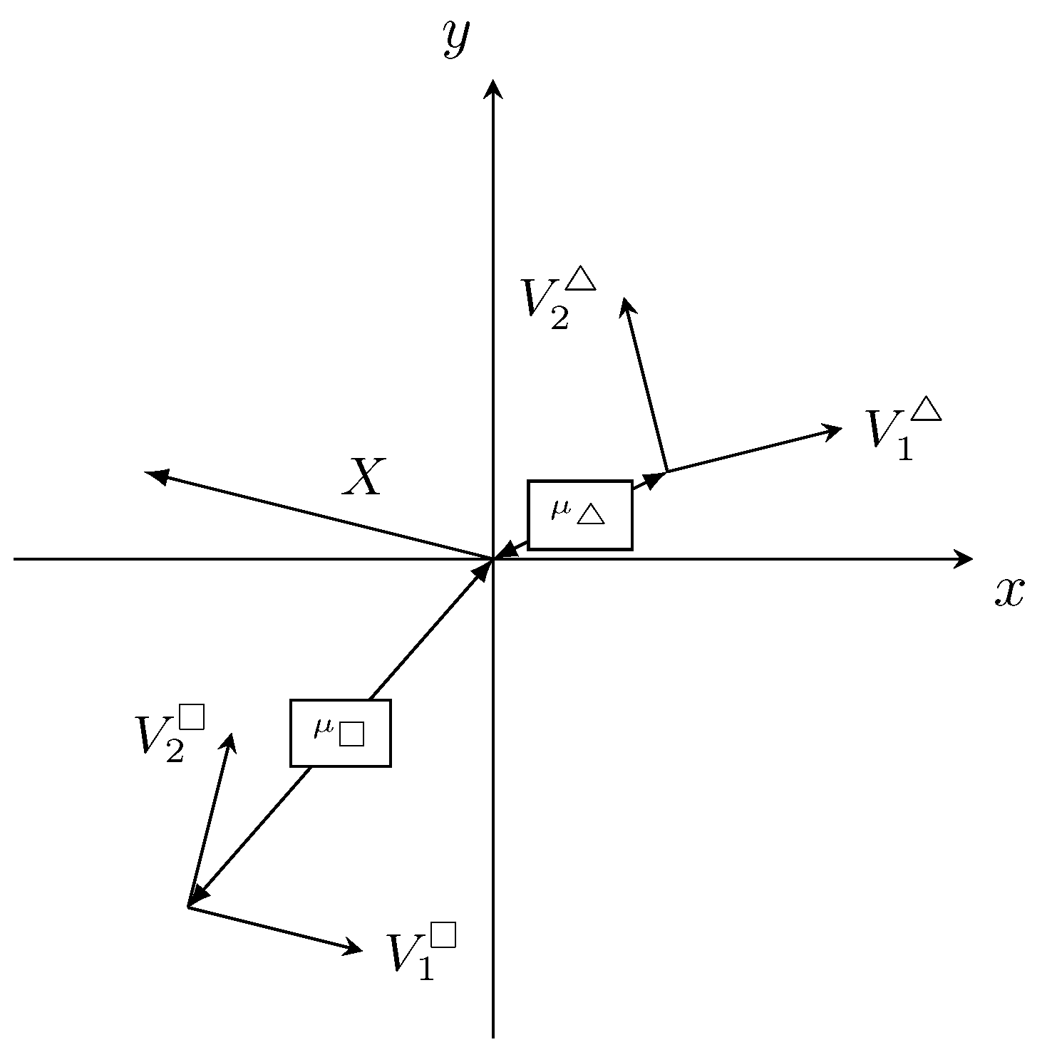
Figure 2.
Illustration of basic steps we used to generate point clouds from colour images (left). First, we just use one colour channel (middle left) and transform it into a black-and-white image (middle right). As the last step, we use the MATLAB routine bwboundaries to create a point cloud (right), see also [24].
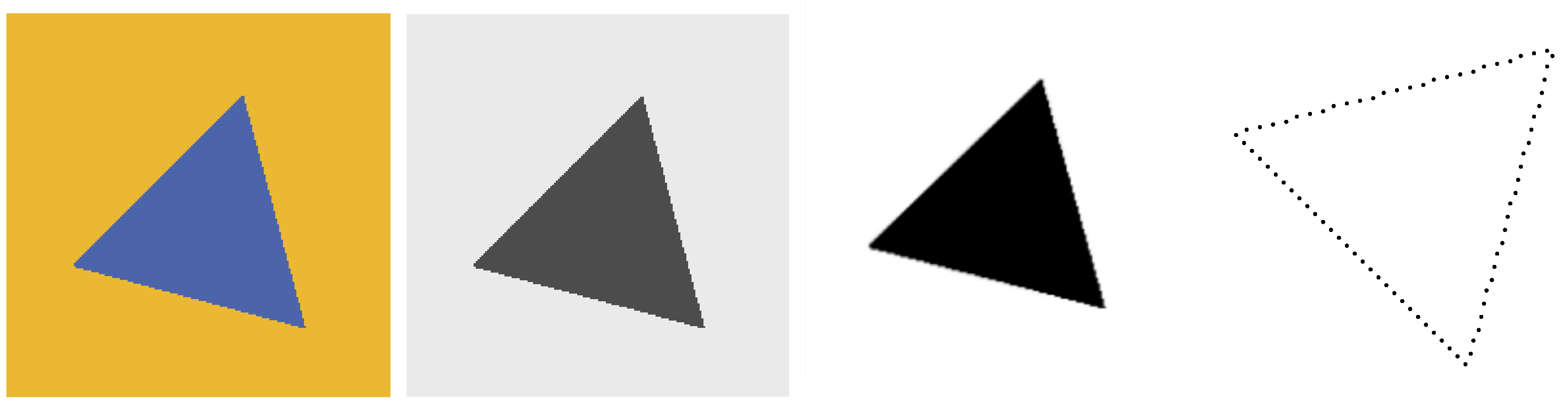
Figure 3.
The visualization of a triangle point cloud, the centre point and the distance d.
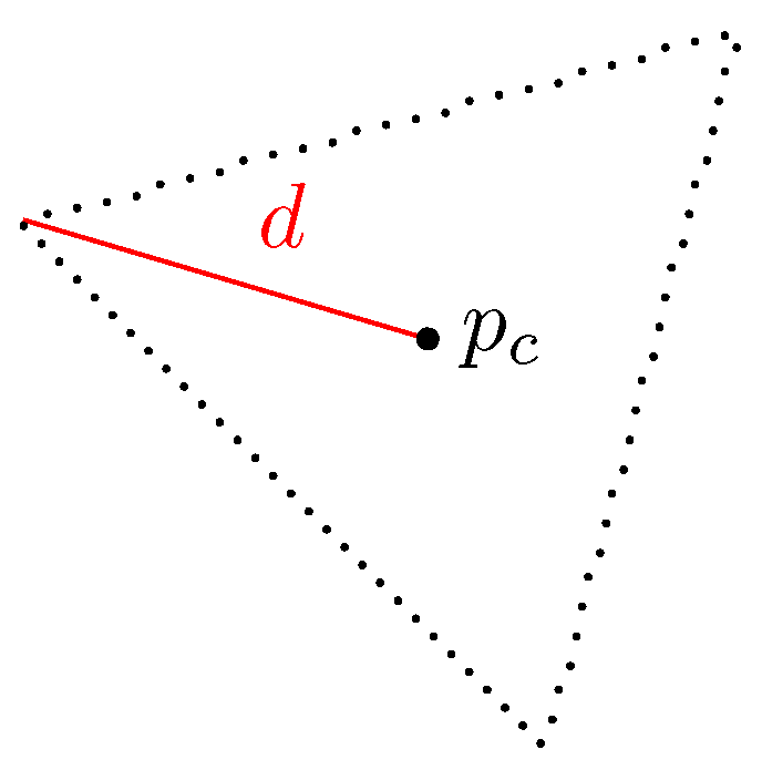
Figure 4.
We plotted here the ordered samples D for four geometrical shapes. The y-axis shows the distance, and the x-axis is just an integer that indicates the position in the sample. Therefore, we left the x-axis empty. From top to bottom, we see the samples of a triangle, pentagon, nonagon, and circle. Additionally, we show the resource images of the samples on the right side. Compare [24].
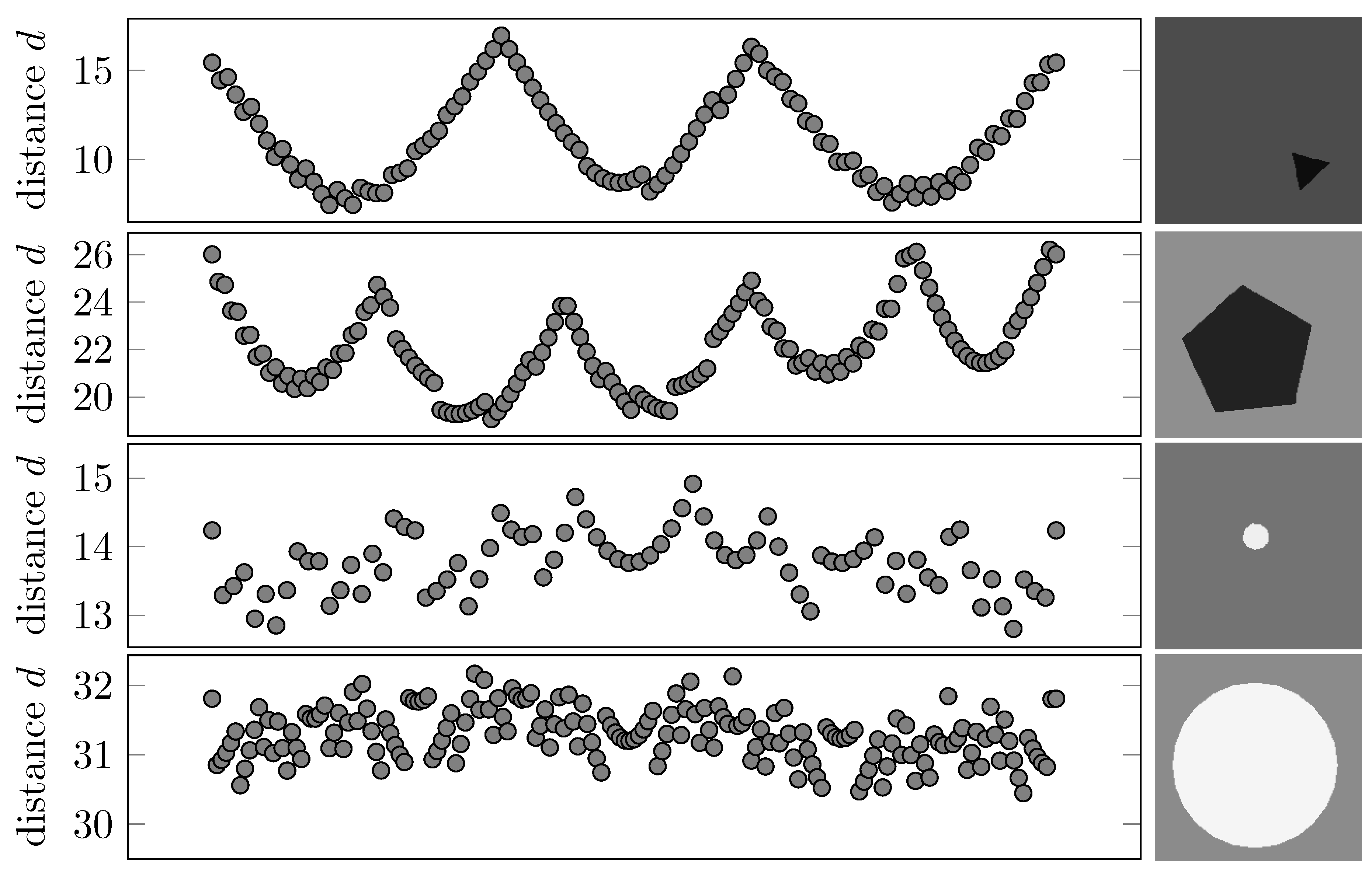
Figure 5.
The square of principal components (left) and (right). We notice that a normalized triangle histogram X to a triangle eigenvector base will produce larger percentages in the first few components than the normalized triangle histogram that act on the eigenvector base of a square.
Figure 5.
The square of principal components (left) and (right). We notice that a normalized triangle histogram X to a triangle eigenvector base will produce larger percentages in the first few components than the normalized triangle histogram that act on the eigenvector base of a square.
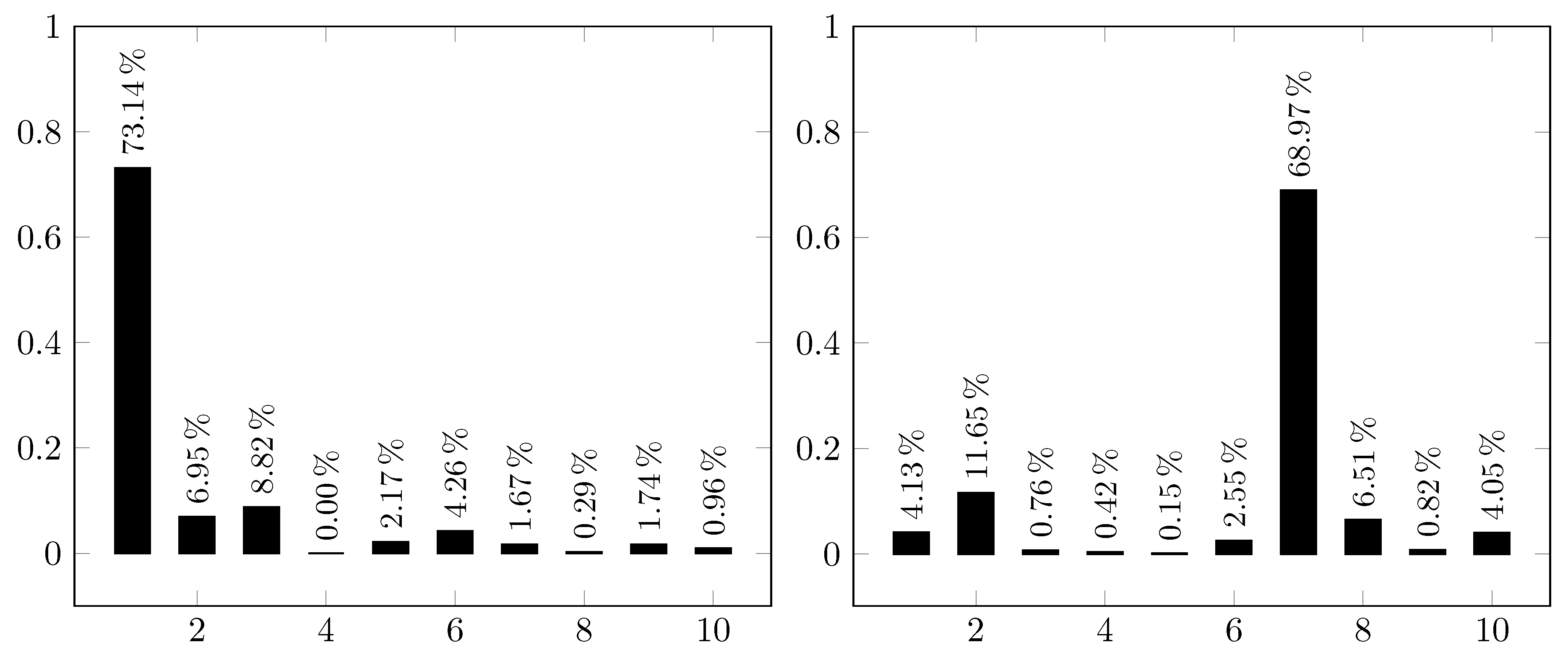
Figure 6.
The visualization of a hit rate matrix . The y-axis show the source shape class and the x-axis present the result of the classification process, e.g. shape class , for . We illustrate the percentage as a grey valued box. Values closer to one, respectively 100%, yield darker boxes, and lighter boxes indicate lower percentages.
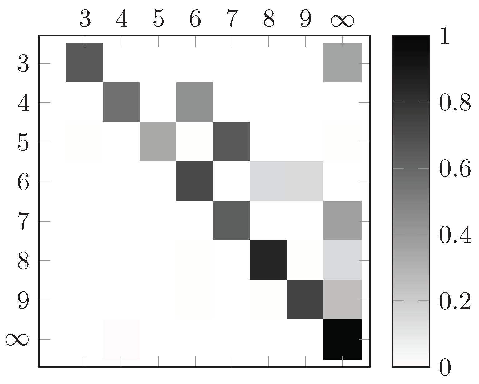
Figure 7.
Hit rate matrices for different values of , . Row-wise, from the top left image down to the bottom right image, we are increasing the value . Starting at one and ending at nine. The samples D were normalized with the mean-Normalization.
Figure 7.
Hit rate matrices for different values of , . Row-wise, from the top left image down to the bottom right image, we are increasing the value . Starting at one and ending at nine. The samples D were normalized with the mean-Normalization.
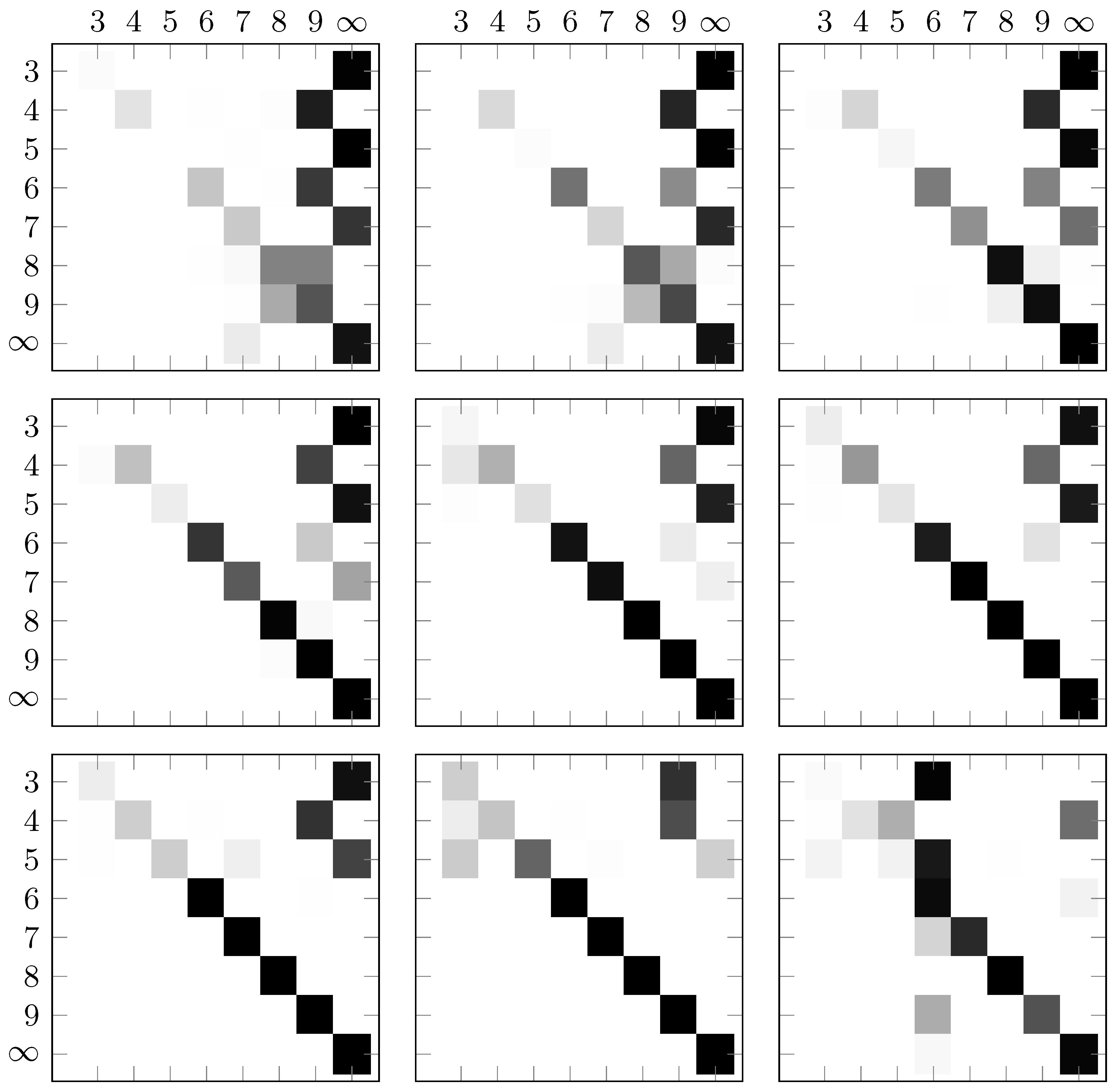
Figure 8.
Hit rate matrices for different values of , . Row-wise, from the top left image down to the bottom right image, we are increasing the value . Starting at one and ending at nine. The samples D were normalized with the max-Normalization.
Figure 8.
Hit rate matrices for different values of , . Row-wise, from the top left image down to the bottom right image, we are increasing the value . Starting at one and ending at nine. The samples D were normalized with the max-Normalization.
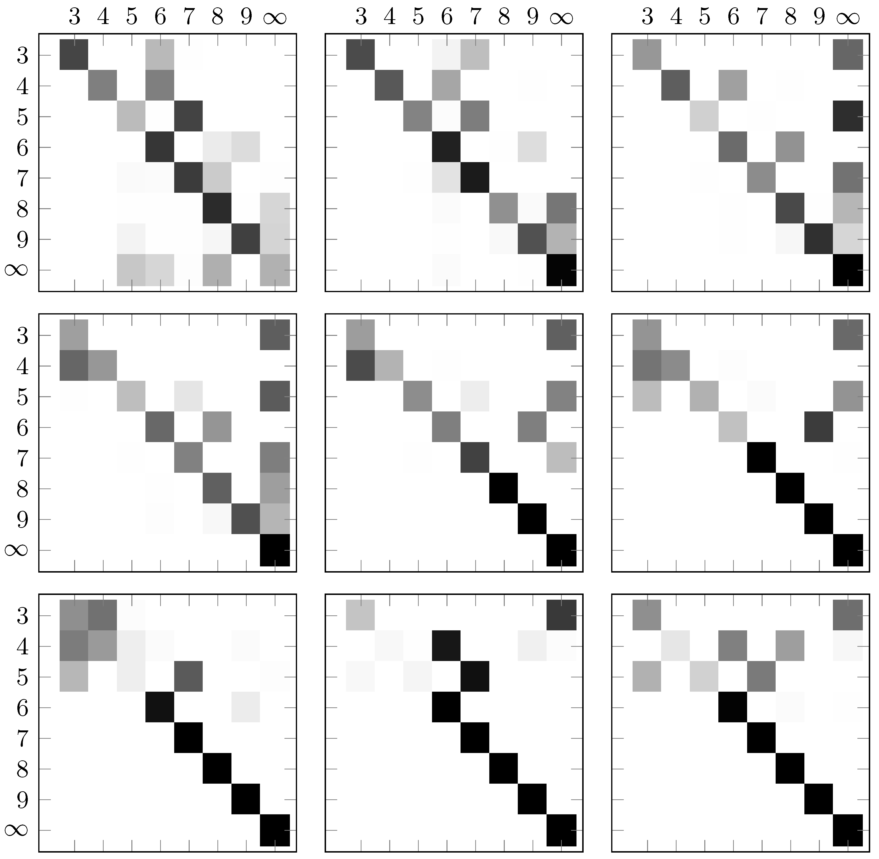

Table 1.
The probabilities of a triangle random vector () acting on different projection operators over different values for . In the second row we used the projector obtained from the triangle eigenvector space and in the third row we make use of the projector from the square shape eigenvectors. For all values of , the second row stores the higher values, which would lead to the conclusion that X is obtained from a triangle point cloud.
| 1 | 2 | 3 | 4 | 5 | 6 | 7 | 8 | 9 | |
| 73.14 | 80.09 | 88.91 | 88.91 | 91.08 | 95.35 | 97.01 | 97.30 | 99.04 | |
| 4.13 | 15.78 | 16.54 | 16.96 | 17.11 | 19.66 | 88.63 | 95.14 | 95.96 |
Disclaimer/Publisher’s Note: The statements, opinions and data contained in all publications are solely those of the individual author(s) and contributor(s) and not of MDPI and/or the editor(s). MDPI and/or the editor(s) disclaim responsibility for any injury to people or property resulting from any ideas, methods, instructions or products referred to in the content. |
© 2024 by the authors. Licensee MDPI, Basel, Switzerland. This article is an open access article distributed under the terms and conditions of the Creative Commons Attribution (CC BY) license (http://creativecommons.org/licenses/by/4.0/).
Copyright: This open access article is published under a Creative Commons CC BY 4.0 license, which permit the free download, distribution, and reuse, provided that the author and preprint are cited in any reuse.


