Integrated Performance of a Modular Biomass Boiler with a Combined Heat and Power Industrial Rankine Cycle and Supplementary sCO2 Brayton Cycle

Preprint

Article

Integrated Performance of a Modular Biomass Boiler with a Combined Heat and Power Industrial Rankine Cycle and Supplementary sCO₂ Brayton Cycle

Altmetrics

Downloads

139

Views

Comments

This version is not peer-reviewed

Submitted:

13 February 2024

Posted:

15 February 2024

You are already at the latest version

Alerts

Abstract

In this paper, the integrated performance of a modular biomass boiler with an existing industrial Rankine steam heat and power cycle and a supplementary supercritical-CO2 (sCO2) Brayton cycle is analyzed. The aim is to leverage the high efficiency supplementary sCO2 cycle to increase net generation and energy efficiency from the existing biomass boiler. Two sCO2 heater configurations situated within the flue gas flow path are investigated, namely a single convective-dominant heater, and a dual heater configuration with a radiative and a convective heater. A quasi-steady-state 1D model was developed to simulate the integrated cycle, including detailed component characteristics for the Rankine and Brayton cycles. The model solves the mass, energy, momentum, and species balance equations. The system is analyzed for three cases: (i) the existing Rankine cycle without the sCO2 integration, (ii) with the single convective-dominant sCO2 heater configuration, and (iii) the dual sCO2 heater configuration. The results show the required rate of overfiring for the sCO2 configurations, with a 15.3% increase in fuel flowrate resulting in an additional 21.2% in net power output. The model quantifies the impact of the sCO2 heaters, with reduced heat uptakes for downstream boiler heat exchangers. Furnace water wall heat uptake increased due to overfiring, offsetting the reduced heat uptakes at downstream evaporative heat exchangers. The dual configuration has more impact on Rankine cycle operation due to the radiative sCO2 heater placement in front of the second superheater, absorbing some of the direct radiation from the furnace.

Keywords:

Subject: Engineering - Mechanical Engineering

1. Introduction

Fossil fuels are currently the world’s largest source of energy [1]. However, there are growing concerns about global warming, unsustainability, and increasing greenhouse gas emissions from the use of fossil fuels. The International Energy Agency (IEA) has outlined a roadmap for net-zero emissions by 2050, where 90% of electricity production is predicted to come from renewable sources [2]. Biomass is a renewable, cost-efficient, carbon-neutral fuel obtained from agricultural waste streams or energy crops that can be combusted in a furnace to co-generate electricity and process heat. Biomass combustion also has benefits for distributed or embedded generation due to the availability and proximity to fuel sources [3]. Biomass fuel is typically used to generate electricity through various Rankine-type steam cycles. However, supercritical carbon dioxide (sCO2) Brayton power cycles have been identified as a potentially attractive technology with a small physical footprint and improved thermal efficiency compared to Rankine cycles, reducing initial capital and operating expenditure [4].

Energy efficiency plays a key role in net-zero emissions by 2050 [2] and the integration of high efficiency supplementary cycles with existing generation systems can potentially increase energy efficiency and net generation. For existing industrial Rankine cycles, increasing generation capacity poses challenges, particularly with large capital expenditure requirements and potential boiler limitations. This is further exacerbated by the relatively low thermal efficiency of industrial Rankine cycles. Retrofitting an existing modular boiler with a high efficiency supplementary sCO2 power cycle may prove to be more economical regarding capital expenditure as well as overall thermal efficiency. The reduced physical footprint of sCO2 power cycles is particularly beneficial when incorporating a supplementary sCO2 power cycle in existing generation systems. However, the integration of these cycles also presents challenges related to component specifications and operating philosophies.

Several studies have focused on cycle-level applications with biomass-fired boilers, with an emphasis on cycle components and simplified models for boiler components [5,6,7]. To capture the impacts of integrating an sCO2 Brayton cycle with an existing biomass fired boiler, a detailed 1D boiler modelling methodology is required. Chatasiriwan [8] explored the optimum installation of various boiler heat exchangers for a biomass boiler. The 1D model considered detailed component sizing and its effects on boiler performance, and solved mass and energy balance equations for the fuel, air, and flue gas streams. Laubscher and De Villiers [9] developed an integrated 1D model of a 105 t/h bagasse-fired industrial water tube boiler in Southern Africa with varying fuel moisture content. The model accounted for detailed heat transfer in the boiler heat exchangers and solved the mass, energy, and momentum balance equations for the water/steam, flue gas, and air streams. A moving-grate stoker boiler was modelled with two superheaters, a spray-type desuperheater, evaporator tube bank, air heater, and economizer. The model was validated with site data as well as CFD results.

sCO2 Brayton cycles have garnered significant research interest, and have been researched for a wide range of applications, including nuclear [10], solar [11], and waste heat recovery [12]. 1D modelling is also used extensively to characterize sCO2 Brayton cycles due to its computational efficiency when analysing and optimising various cycle layouts [13,14,15,16]. sCO2 Brayton cycles have been explored as a viable supplementary cycle for several applications, including biomass fuelled systems [12,17,18,19]. Some studies have looked at using sCO2 as a supplementary cycle with biomass-fuelled systems through direct combustion. Manente et al. [20] proposed a biomass-to-power conversion system based on cascaded sCO2 Brayton cycles. A 1D high-level cycle model was used to explore a combination of cascaded cycle configurations to maximise flue gas heat recovery.

Mutlu et al. [21] developed a hybrid system incorporating a geothermal power plant with a topping sCO2 and bottoming Rankine combined cycle fuelled by olive residue biomass. The bottoming Rankine cycle utilized waste heat rejected from the sCO2 topping cycle, as was the existing turbine from the geothermal system. A 1D steady state model of the combined cycle was developed for the nominal operating point. Zignani et al. [22] performed a preliminary feasibility study on the application of sCO2 power cycles to biomass-fired power plants. An existing 16 MW_e power plant using a Rankine cycle fuelled by woody biomass burnt in a moving-grate stoker boiler was selected as a case study. The proposed sCO2 cycle was intended to replace the Rankine cycle. A 1D steady state model was developed for both the Rankine cycle and various sCO2 cycle configurations.

These studies provide valuable insights into the integration of sCO2 power cycles with biomass boilers. However, the analyses include high level lumped parameter component models, with limited focus on detailed boiler modelling. Additionally, to the author’s knowledge, there have not been any studies focusing on sCO2 cycles integrated with an existing cycle in the same biomass boiler. Further investigation is therefore warranted, specifically looking at the integration of an sCO2 Brayton cycle with a combined heat and power Rankine cycle, and the effects on boiler operation. Using a high detail 1D model capable of capturing complex boiler heat transfer as well as detailed component characteristics for the various cycles is key to understanding the proposed integrated cycle behaviour.

In this paper, a conventional combined heat and power Rankine cycle without sCO2 integration, as well as with integration of two sCO2 Brayton cycle layouts are analysed and compared. The Brayton cycle layouts differ only in terms of its heater configurations, namely a single convective heater configuration, and a dual radiative-convective heater configuration. The heaters for the supplementary sCO2 Brayton cycle are situated in the flue gas flow path inside the boiler. A 1D thermofluid process model is developed and applied to investigate the three cycle layouts with a biomass-fired boiler. The novelty of the proposed research lies with the proposed integrated cycle, as well as the complexity of the developed 1D model. To the best of the author’s knowledge, the integration of an sCO2 cycle with an existing industrial Rankine cycle in the same biomass boiler has not previously been investigated. The study also focuses on Southern African bagasse as the fuel source, which provides perspective on the applicability of the proposed integrated cycle for the region. While works of similar nature focus on simple thermodynamic analyses through mass and energy balances, the present work solves the momentum balance equations in addition to mass and energy balances. This requires detailed component characteristics, including performance curves for turbomachinery, and allows for quasi-steady-state analysis for nominal and part loads.

2. Cycle Layout and Operation

The case study existing biomass boiler is a compact modular grate-fired boiler, accommodating a wide range of fuels, such as bagasse which is the fuel used for this study. The boiler is rated at approximately 35 MW_th nominal heat generation, heating steam to 485°C at 69 bar. Schematics of the boiler geometry with the proposed single and dual sCO2 heater configurations included are shown on the left and right of Figure 1. The green arrows indicate the combustion air inlets and the black arrows the fuel inlet, while the red arrows indicate the flue gas flow path. For the existing cycle without the sCO2 Brayton cycle integration, the schematic remains the same, except for the presence of the sCO2 heaters (shown in grey). Additionally, process flow diagrams of the integrated cycle for the single and dual sCO2 heater configurations are shown in Figure 2 and Figure 3 respectively. Likewise, the process flow diagram for the existing cycle without the integration does not include the sCO2 heaters.

Evaporative water-walls fed by the steam drum via the downcomer pipe surrounds the furnace and other heat exchangers. There are two in-line steam superheaters (SH1 and SH2), an indirect attemperator, top and bottom evaporator tube banks (tEV, bEV), two heat exchanger screens (SCR1, SCR2), two cavities (CAV1 - split into tCAV1, bCAV1, and CAV2), several tubular air-heaters (tAH, bAHt, bAHb), and three economizer heat exchangers (EC1, EC2, EC3).

Fuel, in this case bagasse, is distributed via distribution air onto a moving grate which transports the fuel to the furnace rear. Heated primary and secondary combustion air streams respectively are injected from below through the grate and directly into the lower furnace volume. The bagasse has a higher heating value (HHV) and lower heating value (LHV) of 8838

kJ / kg

and 7165

kJ / kg

respectively, with as-received ultimate analysis shown in Table 1. An excess air percentage of 27% is assumed, with bagasse boiler furnaces typically using an excess air percentage of 25-35% [23].

The industrial Rankine cycle consists of the components shown in the process flow diagrams in Figure 2 or Figure 3. The BFP pumps the main feedwater through the boiler, including the economizers, water walls, evaporators, attemperator, and superheaters. Additionally, there are valves to allow for control of the Rankine cycle for various operating conditions. These include the BFP valve, turbine valve, process heat valve, and bypass valve. Power is generated by the HPT and LPT. The main flow stream splits after the HPT into the process heat line and the LPT. Process heat is provided according to the required demand. For this study, it is assumed that the process heat demand is fixed at 2 MW and water returning from the external process is saturated liquid. Moreover, a bypass line exists in parallel with the process heat line to allow for additional steam flow directly to the de-aerator. The steam flow through the LPT passes through the condenser where it is cooled by 1000 kg/s of cooling water provided at 25°C. The CFP then pumps the condensate into the de-aerator, where the process heat and bypass lines also connect.

For this study a simple recuperated sCO2 Brayton cycle layout is selected. It includes a single compressor and turbine, recuperator, pre-cooler, and direct attemperator as shown in the process flow diagrams (Figure 2 or Figure 3). High-pressure sCO2 from the compressor outlet splits into two flow streams, with the majority flowing to the high-pressure side of the recuperator (RXHP) and the remaining going to the direct attemperator. From the turbine outlet, high temperature sCO2 on the low-pressure side of the recuperator (RXLP) heats up the sCO2 at the RXHP. sCO2 then enters the pre-cooler, where it is cooled by 500 kg/s of cooling water at 25°C. The sCO2 is cooled to 33°C at 10 MPa, which are the compressor inlet conditions.

Boiler heat exchangers are modelled as tube bank heat exchangers. For the single heater sCO2 Brayton cycle configuration, the boiler schematic and process flow diagram can be seen on the left of Figure 1 and in Figure 2. The single heater is positioned in CAV1, splitting the cavity into tCAV1 and bCAV1. It is important to include attemperation in the sCO2 cycle, allowing for temperature control at the heater outlet, i.e., the turbine inlet. For the single heater configuration, a portion of the flow bypasses the RXHP and is then mixed with the sCO2 heated in the RXHP, from where it flows into the sCO2 heater. The dual heater configuration, shown on the right of Figure 1 and in Figure 3, utilises two sCO2 heaters. The first heater, sCO2H1, is a platen radiative heat exchanger, positioned in front of SH2. The second heater, sCO2H2, is like the heater in the single heater configuration and is positioned between tCAV1 and bCAV1. Attemperation for the dual configuration takes place between sCO2H1 and sCO2H2, with a portion of the flow bypassing sCO2H1 and is then mixed with the sCO2 heated in sCO2H1.

The high flue gas temperatures (>700°C) allow for high maximum sCO2 Brayton cycle temperatures. Consequently, three turbine inlet temperatures (TIT) were initially explored, namely 550°C, 650°C and 720°C. A parametric study was conducted for the three TITs using initial sCO2 heater specifications. The sCO2 heater specifications were then tuned for the selected 550°C TIT, shown in Table 2. An iterative design process was used to select heater specifications to ensure that the Rankine cycle performance is not adversely impacted. TP347HFG was selected for the sCO2 tube bank material, typically used for superheaters in supercritical boilers. The tube outer diameter and thickness are selected from standard ASTM sizes based on an allowable material stress (30 MPa fluid pressure) at 700°C.

The transverse pitch,

S_{t}

, is fixed at 0.2m due to boiler spacing constraints. For the dual heater configuration, the width and height of sCO2H1 is based on the geometry of SH2. The geometry for sCO2H2 is limited by the size of CAV1, particularly the width and height of the heat exchanger tube bundle. The duct length,

L_{d u c t}

, and longitudinal pitch,

S_{l}

, were adjusted iteratively for both sCO2H1 and sCO2H2. sCO2H1 is modelled as a platen heat exchanger due to the small longitudinal pitch compared to the tube outer diameter. For the single heater configuration, similar to sCO2H2, the geometry is limited to the space available in CAV1, and the same geometric parameters are determined (

L_{d u c t}

S_{l}

). By adjusting

L_{d u c t}

for sCO2HX and sCO2H2, the lengths of tCAV1 and bCAV1 are also adjusted. For comparison purposes, the heater geometries are determined to ensure that both heater configurations are simulated with similar fuel flow rates. For the conventional cycle without sCO2 integration, CAV1 is equally split to form tCAV1 and bCAV1.

3. Thermofluid Network Model

The proposed 1D system model uses a thermofluid network modelling approach similar to Rousseau et al. [24], which has been validated with site data of an industrial-scale biomass-fired boiler. It solves the 1D incompressible steady state mass, energy, momentum, and species balance equations (Equations (1)–(4) respectively) for the control volumes shown in the process flow diagrams (Figure 2 and Figure 3). A custom-built 1D thermofluid network solver is developed in Python. The solver adopts a node and element methodology, where each element is connected to an inlet and outlet node. Fluid properties are computed at nodes using the real-fluid CoolProp library [25]. Component characteristics are solved at elements, including

\dot{Q}

and

\dot{W}

for the energy balance, and

Δ p_{0}

for momentum balance. Additionally, mass flow rates are updated at elements. For gas mixtures, Equation (4) is used to ensure species balance for each species constituent, where subscript j is a species constituent.

\sum {\dot{m}}_{e} - \sum {\dot{m}}_{i} = 0

(1)

\sum {\dot{m}}_{e} h_{0 e} - \sum {\dot{m}}_{i} h_{0 i} = \dot{Q} - \dot{W}

(2)

p_{0 e} - p_{0 i} = Δ p_{0}

(3)

\sum {\dot{m}}_{e} Y_{e_{j}} - \sum {\dot{m}}_{i} Y_{i_{j}} = 0

(4)

with the total pressure

p_{0} = p + \frac{1}{2} ρ v^{2} + ρ g z

and total enthalpy

h_{0} = h + \frac{1}{2} v^{2} + g z

The energy balance Equation (2) results in a set of simultaneous equations that can be solved for the total enthalpy at each node. For momentum balance, the component characteristics are written in a generic linearised form of

Δ p_{0} = a_{0} + a_{1} \dot{m}

(5)

This is substituted into the momentum balance Equation (3) to get

\dot{m} = \frac{p_{0 e} - p_{0 i} - a_{0}}{a_{1}}

(6)

This in turn is substituted into the mass balance Equation (1) to get a set of simultaneous equations that can be solved for the total pressure at each node, which also satisfies the mass balance.

For turbomachinery components, polynomial equations are used to compute the pressure ratio for a given non-dimensional flow rate, and in turn, used to compute

Δ p_{0}

. For heat exchangers and pipes, the total pressure change is calculated using:

Δ p_{0} = - \frac{K_{l o s s}}{2 ρ_{a v g} A^{2}} | \dot{m} | \dot{m}

(7)

An iterative solution procedure is used to enforce the balance equations for each flow stream. Relaxation is applied in the solution of node enthalpies and pressures to ensure numerical stability. Fluid properties and component characteristics are then updated using the newly calculated enthalpies and pressures and the solver repeats till convergence. A relative convergence of 1E-6 is used for pressures, and 1E-4 for enthalpies. The thermofluid solver has been thoroughly verified. Component characteristic sub-component models have been verified using similar models developed in Mathcad and Python, with agreement within 2%. Additionally, the implementation of the balance equations has also been verified using Flownex^®, which is a commercial 1D thermofluid solver.

The following sub-sections describe the component characteristics and modelling methodology for the cycle components shown in the process flow diagrams in Figure 2 and Figure 3.

3.1. Boiler

3.1.1. Combustion

The combustion model is based on the assumption of instantaneous combustion (i.e., not accounting for the kinetics) with an assumed fraction of unburned carbon. The inputs to the combustion model include the HHV, fuel composition, fuel temperature, fuel mass flow rate, air temperature and absolute humidity, fly-ash fraction, excess air ratio, and the fractional distribution of air across primary, secondary, and distribution streams. The combustion air flow rate, flue gas flow rate and flue gas composition are determined from the species mass balance as described in Rousseau et al. [24].

An energy balance is conducted over the combustion zone control volume to determine the adiabatic flame temperature, assuming all the combustion heat is released in the furnace control volume. Equation (8) shows the energy balance equation. Fly-ash is not explicitly included in the gas-mixture, however, is accounted for during radiation heat transfer as well as energy balances in the

\begin{matrix} {\dot{m}}_{F G} h_{F G_{A F T}} + {\dot{m}}_{F A} c_{P_{a s h}} (T_{A F T} - T_{r e f}) = {\dot{m}}_{f u e l} (c_{P}_{f u e l} (T_{f u e l} - T_{r e f}) + H H V_{f u e l} - Y_{f u e l_{U C}} H H V_{C}) + \\ {\dot{m}}_{P A} h_{P A} + {\dot{m}}_{S A} h_{S A} + {\dot{m}}_{D A} h_{D A} \end{matrix}

(8)

As the adiabatic flame temperature (

T_{A F T}

) is initially unknown, an iterative procedure is used to satisfy Equation (8), accounting for the flue gas and fly ash exiting the combustion control volume, as well as fuel, unburned char, and various air supply streams entering the control volume. In Equation (8),

c_{P, a s h} = 710 J / kgK

c_{P, f u e l} = 1200 J / kgK

T_{r e f} = 298.15 ​ K

and

H H V_{C} = 32763 kJ / kg

. The enthalpy of flue gas exiting the boiler (

h_{F G_{A F T}}

) is derived from

T_{A F T}

based on the appropriate real gas mixture properties. Primary and secondary air streams are assumed to come from the air heaters and enter the combustion control volume together. Ambient distribution air also feeds into the combustion control volume. The fractions of these air streams are

f_{P A} = 0.508, f_{S A} = 0.402, f_{D A} = 0.090

. The mass flow rates of the air streams are then computed using the respective fraction split and the total combustion air mass flow rate,

m_{c a}

3.1.2. Furnace

The furnace is dominated by radiative heat transfer to the furnace water walls. The Gurvich method [26] is used to calculate the projected radiative heat transfer from hot gases and particles to the furnace water walls, as well as the furnace exit temperature. Equation (9) shows the empirical formula for calculating the furnace exit gas temperature.

T_{F G, F E} = \frac{T_{A F T}}{M_{f l a m e} {\frac{ϵ_{e f f, f u r}}{B o}}^{0.6} + 1}

(9)

The flame modification factor M is calculated as:

M = A' - B' (X_{r} + ​ Δ X)

(10)

In Equation (10), for the present study with a grate-fired bagasse boiler,

A' = 0.59

B' = 0.59

, and

(X_{r} + ​ Δ X) = 0.14

[27]. Bo, the Boltzmann number, in Equation (9) is calculated as:

B o = \frac{ϕ_{f u r} {\dot{m}}_{f u e l} V \bar{C}}{σ_{0} ψ A_{r a d, f u r} T_{A F T}^{3}}

(11)

In Equation 10,

V \bar{C}

is the mean overall heat capacity of flue gas per kg of fuel,

ϕ_{f u r} = 1 - f_{r a d l o s s}

where

f_{r a d l o s s} = 0.0101

A_{r a d, f u r}

is the projected radiative furnace area accounting for the angular coefficient at the tube walls, refractory walls, furnace exit, and grate.

ψ

is the area weighted furnace efficiency factor, accounting for the angular coefficient, geometric arrangement, and fouling factors of furnace surfaces. From Equation (9),

ϵ_{e f f, f u r}

is the effective gas emissivity in the furnace, calculated using the approach by Brummel [28], considering high particulate loading and radiation scattering as described in [24]. The furnace gas emissivity is influenced by tri-atomic gas radiation, coke particle radiation, ash particulate absorption and radiation scattering. Flue gas tri-atomic emissivity is computed using the weighted-sum-of-gray-gas model. Once

T_{F G, F E}

from Equation (9) has been computed, the heat transfer in the furnace control volume is computed using:

{\dot{Q}}_{F G, f u r} = {\dot{Q}}_{F E} + {\dot{Q}}_{f u r, l o s s} + {\dot{Q}}_{W W} + ​ {\dot{Q}}_{R F}

(12)

{\dot{Q}}_{F G, f u r}

is evaluated using an energy balance over the furnace control volume, shown in Equation (13). The energy balance accounts for flue gas and fly-ash particles, using the calculated furnace exit gas temperature and the adiabatic flame temperature calculated at the combustion control volume.

{\dot{Q}}_{F G, f u r} = {\dot{m}}_{F G} (h_{F G, A F T} - h_{F G, F E}) + {\dot{m}}_{F A} (h_{F A, A F T} - h_{F A, F E})

(13)

{\dot{Q}}_{F E} = β_{F E} η_{F E} A_{F E} \frac{{\dot{Q}}_{f u r} ϕ_{f u r}}{A_{e f f, f u r}}

(14)

{\dot{Q}}_{R F} = η_{R F} A_{R F} \frac{{\dot{Q}}_{f u r} ϕ_{f u r}}{A_{e f f, f u r}}

(15)

{\dot{Q}}_{f u r, l o s s} = (1 - ϕ_{f u r}) {\dot{Q}}_{f u r}

(16)

{\dot{Q}}_{F E}

is the direct radiation leaving at the furnace exit plane and is evaluated using Equation (14), where

β_{F E}

is an empirical re-radiation coefficient dependent on the furnace exit temperature,

η_{F E}

is the coefficient of heat flux non-uniformity at the furnace exit determined by empirical curves along the furnace height,

A_{F E}

is the projected furnace exit area, and

A_{e f f, f u r}

the total effective projected furnace area.

{\dot{Q}}_{R F}

is the heat transfer at the refractory covered walls in the furnace evaluated using Equation (15).

{\dot{Q}}_{f u r, l o s s}

is calculated in Equation (16), and consequently the water wall heat transfer

{\dot{Q}}_{W W}

is calculated using Equation (12) with all other variables known.

3.1.3. Boiler Heat Exchangers

Boiler heat exchangers include radiative-convective heat exchangers, evaporators, screens, and cavities. Radiative and convective heat transfer is modelled for each heat exchanger, as well as to water walls surrounding the heat exchanger. Flue gas control volumes are explicitly modelled for each heat exchanger, as shown in the process flow diagrams in Figure 2 and Figure 3. A lumped control volume for the water side, EV, is used to capture heat transfer to the water walls, cavities, evaporators, and screens. Geometric parameters, such as those described for the sCO2 heater in Table 2, are specified for each boiler heat exchanger.

Radiative-convective tube bank heat exchangers include superheaters (SH1, SH2), sCO2 heaters (sCO2HX, sCO2H1, sCO2H2), economizers (EC1, EC2, EC3), and air heaters (tAH, bAHt, bAHb). For radiative-convective heat exchangers, the secondary fluid stream (water/CO2/air) is explicitly modelled and coupled to the corresponding flue gas control volume for heat transfer modelling. Figure 4 shows the generic heat transfer flow diagram for radiative-convective heat exchangers.

Fly-ash in the gas stream is accounted for in the energy balance for the flue gas volume using the inlet and outlet flue gas temperatures,

c_{P, a s h} = 710 J / kgK

, and

{\dot{m}}_{f a}

calculated at the combustion control volume. For flue gas, the gas and particulate mixture emissivity is again calculated using the approach by Brummel [28] described in the furnace section.

{\dot{Q}}_{r i}

is the heat transfer rate of incoming direct radiation from up-stream gas flows. For example, at SH2 which is downstream the furnace control volume,

{\dot{Q}}_{r i, S H 2} = {\dot{Q}}_{F E} = {\dot{Q}}_{r e, f u r}

. Absorbed radiation,

{\dot{Q}}_{a b s}

, is the difference between

{\dot{Q}}_{r i}

and bypassing radiation

{\dot{Q}}_{b y p a s s}

[29]. The outgoing direct radiation from the heat exchanger,

{\dot{Q}}_{r e}

, is made up of

{\dot{Q}}_{b y p a s s}

and additional gas radiation leaving the outlet plane of the heat exchanger,

{\dot{Q}}_{b a c k}

, calculated using Equation (17).

{\dot{Q}}_{b a c k} = 0.5 ϵ_{f g} σ_{0} A_{H X o u t} T^{4}_{f g, a v g}

(17)

Heat transfer for radiative-convective heat exchangers is dominated by two mechanisms, namely gas and particulate radiation, and forced convection from the flue gas surrounding the tube bank. Figure 5 shows the thermal resistance network that characterise the heat exchanger tubes.

The combined flue gas external heat transfer coefficient,

h_{f g}

, is the sum of the convective heat transfer coefficient,

h_{f g, c o n v}

, and gas radiative heat transfer coefficient,

h_{f g, r a d}

h_{f g, r a d}

is calculated using the radiative heat flux from the flue gas to the outer fouling layer of the heat exchanger tubes.

\begin{array}{l} h_{f g, r a d} = \frac{q_{f g, r a d}}{T_{f g, a v g} - T_{f o}} \\ q_{f g, r a d} = \frac{ϵ_{f o} + 1}{2} σ_{0} ϵ_{f g, i} (T^{4}_{f g, a v g} - T_{f o}^{4}) \end{array}

(18)

ϵ_{f o}

is the emissivity of the outer ash layer on the tubes, set to 0.8, typically used for solid-fuel fired boilers [27]. The external forced convection heat transfer coefficient,

h_{f g, c o n v}

, is calculated using correlations by Gnielinski [30]. For internal forced convection of the secondary fluid,

h_{\sec}

, the Gnielinski turbulent convection correlation is used [31]. An outer and inner fouling layer around the tube walls is accounted for in the model.

R_{f o}

is the thermal resistance due to ash deposits on the tube bank, set to

0.0043 \frac{m^{2} K}{W}

[27]. The inner fouling thermal resistance is assumed to be negligible. For air heaters, a utilization factor,

ψ_{H X, A H} = 0.9

, is applied to impose fouling thermal resistances, while the utilization factor is set to 1 for other boiler heat exchangers. A balance between the internal heat transfer rate to the secondary fluid,

{\dot{Q}}_{\sec}

, and the external heat transfer rate from the flue gas and absorbed direct radiation,

{\dot{Q}}_{e x}

and

{\dot{Q}}_{a b s}

is obtained via iteration while varying the outer surface temperature of the fouling

T_{f o}

. The external overall heat transfer coefficient and effectiveness-NTU method is used to calculate

{\dot{Q}}_{e x}

. Similarly,

{\dot{Q}}_{\sec}

is calculated using the thermal resistances from the outer surface of the fouling to the secondary fluid as shown in Figure 5, including outer and inner fouling layers, and tube wall conduction. For the platen-type sCO2H1, the external surface area of the tubes is adjusted to account for the tubes being modelled as flat plates. Lastly, the outer and inner tube wall metal temperatures,

T_{w o}

and

T_{w i}

are computed using the respective thermal resistances and

{\dot{Q}}_{s e c}

The heat transfer rate to the water walls,

{\dot{Q}}_{w a l l}

, and roof,

{\dot{Q}}_{r o o f}

is calculated using the radiative and convective heat transfer coefficients calculated for flue gas across the tube bank. However, to account for the reduced gas flow velocities surrounding the water walls, the heat transfer coefficient is corrected as shown in Equation (19) using coefficients derived from CFD analyses. The coefficients used are

β_{c o n v} = - 0.678

and

β_{r a d} = 0.375

. Consequently, Equation (20) is used to calculate

{\dot{Q}}_{w a l l}

and

{\dot{Q}}_{r o o f}

A_{w a l l}

is the water wall/roof area surrounding the tube bank, and

T_{w a l l}

is the outside surface temperature of the water walls of the evaporating circuit, which is assumed to be equal to the saturation temperature of the steam, i.e., 285°C.

h_{f g, w a l l} = (1 + β_{c o n v}) h_{f g, c o n v} + (1 + β_{r a d}) h_{f g, r a d}

(19)

{\dot{Q}}_{w a l l} = h_{f g, w a l l} A_{w a l l} (T_{f g, a v g} - T_{w a l l})

(20)

For tubular air heaters, the internal Gnielinski correlation is used for flue gas, while the external flow correlations are used for the air stream. Economisers are modelled as radiative-convective heat exchangers as described above. The air heaters and economisers are not surrounded by water walls.

The steam drum separates the incoming flow from the economiser into vapour and liquid streams, modelled as a simple mixture node with two-phase separation. The level control in the drum is simulated by ensuring a fixed quality within the drum. An external control loop is used to ensure energy balance across the steam drum while maintaining the drum pressure at 6.914 MPa, explained further in Section 3.4. The attemperator is used to ensure a fixed outlet temperature at SH2 of

485 ° C

by extracting heat as required between SH1 and SH2. The required

{\dot{Q}}_{A T T}

is found iteratively via an external control loop.

3.2. Rankine Cycle

The component characteristics for the turbomachinery, including the CFP, BFP, HPT, and LPT, are specified via generic performance curves for the pressure ratio and isentropic efficiency versus normalized mass flow rate. Second-order polynomial curves of the form

a_{0} + a_{1} C M_{C / T} + a_{2} C M_{C / T}^{2}

are used for Rankine cycle turbomachinery. These performance curves determine the Rankine cycle feedwater flowrate, provided by the BFP, as well as the performance of the turbomachinery through the isentropic efficiency performance curves. For turbines, the isentropic efficiency is assumed to be 0.7 and 0.6 for the HPT and LPT respectively, observed in literature for similar steam conditions [32,33,34], and 0.65 for pumps. Valve components are modelled as simple 1D pipe components with a secondary loss factor,

K_{v a l v e}

. For various valves,

K_{v a l v e}

is iteratively tuned to satisfy a selected target function.

In this study, an assumed fixed amount of process heat, 2 MW, is extracted at the process heat line, with the flow returning from the process as saturated liquid. The external control loop ensures an energy balance for the process heat line. The de-aerator is modelled like the steam drum, with only a saturated liquid outflow. The pressure at the de-aerator is fixed at

835 kPa

, and a mass balance across the de-aerator is enforced via an external control loop, discussed further in Section 3.4. The condenser is modelled as a heat exchanger with a fixed UA value. The

ε - NTU

method is used to model heat transfer between the incoming steam and ambient cooling water in a counter-flow arrangement.

3.3. Brayton Cycle

Turbomachinery for the Brayton cycle is also modelled using generic performance characteristic curves for pressure ratio and isentropic efficiency, captured using the normalized mass flow rate shown in Equation (21), through 4th order polynomials,

a_{0} + a_{1} C M_{C / T} + a_{2} C M_{C / T}^{2} + a_{3} C M_{C / T}^{3} + a_{4} C M_{C / T}^{4}

C M_{C / T} = \frac{\dot{m} \sqrt{T_{0 i}}}{p_{0 i}}

(21)

Detail design of the turbomachines is outside the scope of this study and the compressor pressure ratio performance curve is specified to ensure a pressure ratio of 2.5 at nominal load. The nominal mass flow rate for the Brayton cycle is selected to ensure the chosen turbine inlet temperature (550°C/650°C/720°C). Similarly, isentropic efficiency curves are specified with nominal full load efficiency of 0.9 for both compressor and turbine. A compressor inlet pressure of 10 MPa is selected at the nominal full load operating conditions. This pressure needs to be high enough to ensure that at lower loads the compressor inlet pressure will not be below the sCO2 critical point resulting in liquid entering the compressor.

The recuperator and pre-cooler are both modelled using a pre-defined overall conductance,

U A

value, and detailed geometry is not considered. Due to the large variation in CO2 fluid properties near the critical point, 31°C and 7.1 MPa, it is important to discretize the pre-cooler to capture the considerable change in fluid properties. Similarly, the recuperator is also discretised. A grid independence study was conducted, and a discretization resolution of 6 elements was selected for both recuperator and pre-cooler. The overall conductance is divided equally for each discretized element. The recuperator is sized using

U A_{R X}

, which is selected by ensuring an overall nominal full-load recuperator effectiveness,

ε_{R X}

in Eq.(22), of 0.9 [16]. The pre-cooler is sized using

U A_{P C}

, which is selected to ensure an outlet temperature of

T_{P C, e} = 33 ° C = T_{c o m p, i}

ε_{R X} = \frac{h_{c, e} - h_{c, i}}{h_{h, i} - h |_{p_{h, e}, T_{c, i}}} = \frac{h_{h, i} - h_{h, e}}{h_{h, i} - h |_{p_{h, e}, T_{c, i}}}

(22)

A direct attemperator is used for the sCO2 Brayton cycle. The fraction of the flow stream for attemperation is fixed at 10% for both heater configurations, enforced through a secondary loss factor specified at the attemperator control valve,

K_{A T T}

. The attemperation stream and primary flow stream are then mixed at the attemperation node, modelled as a simple mixing chamber. The sCO2 heaters are modelled as radiative-convective heat exchangers, discussed in section 3.1.3. A 1% pressure drop is assumed for both sCO2 heat exchangers, implemented using specified secondary loss factors.

3.4. Boundary Conditions, Set Points, and Solution Procedure

Geometric parameters and parameters described in the previous section are used to compute component characteristics for various components in the integrated cycle model. Figure 6 shows various inputs and boundary conditions for the integrated cycle model. Component characteristic inputs are as described in the previous section, such as turbomachinery performance curves, and not explicitly shown in the figure. As the model solves the momentum balance equations, set points for various cycle parameters are not enforced directly, and are instead converged to via steady state control. For example, to enforce a mass flow rate for a pipe, the secondary loss factor for that pipe,

K_{l o s s}

, is specified and iteratively tuned via steady state control to obtain the required mass flow rate. While this approach requires steady state control of the integrated cycle, it also captures component characteristics which in turn determine cycle operating points. This is beneficial when simulating various operating conditions and required for part load analysis. In contrast, without solving the momentum balance equations, operating points, such as mass flow rates, must be directly imposed, meaning component characteristics may not necessarily be captured, which is the approach typically used for similar studies observed in literature.

For the boiler, the inputs for the combustion reaction are required, as described in Section 3.1.1. Additionally, ambient pressure and temperature, and air composition is specified. Initially, the combustion reaction is computed for a provided

{\dot{m}}_{f u e l}

, and the calculated mass flow rate for air supply and flue gas streams as well as flue gas composition is used as a boundary condition. This is calculated before the iterative solution process. During the iterative solution,

T_{A F T}

and

T_{F E}

are updated by the combustion and furnace components respectively. The calculated temperatures are applied at each iteration as temperature boundary conditions at the combustion and furnace outlet nodes.

For the Rankine cycle,

p_{c o n d, o u t}

, the

K_{l o s s}

for various valves, and

{\dot{Q}}_{A T T}

for attemperation are specified. The condenser ambient cooling water inlet pressure, temperature, and mass flow rate are also specified.

K_{t u r b}

is used to vary the load of the Rankine cycle. The current study only considers nominal load; therefore, the turbine valve is nominally fully open for all cases. Consequently, overall Rankine cycle performance is similar for all cases. As the sCO2 Brayton cycle is conceptualised as a supplementary cycle, its performance varies based on the Rankine cycle load. For both Brayton cycle configurations, the pre-cooler outlet pressure/compressor inlet pressure is specified at 10 MPa, as well as the ambient cooling water inlet pressure and temperature, and mass flow rate.

Several constraints are applied to the model, shown in red text in Figure 6. To arrive at a fully converged solution where these constraints are satisfied, the iterative solution process is wrapped in an external solver loop. A Newton-Raphson algorithm from the SciPy library is used to find suitable values of parameters to satisfy the respective target functions from these constraints. These parameters are shown in green text in Figure 6. Table 3 shows the control parameters, target functions, and constraints satisfied by the external loop. For each iteration of the external search loop, the balance equations are solved to convergence.

K_{t u r b}

is a primary input to the Rankine cycle model and in this study, the turbine valve is fully opened for full load simulation. Similarly for the Brayton cycle,

p_{P C, o u t}

is also a primary input, fixed at 10 MPa. The controlled parameters in Table 3 are adjusted for full convergence with the provided component characteristics, sCO2 heater geometry,

K_{t u r b}

, and

p_{P C, o u t}

. Effectively, this means that Rankine cycle performance is the same for various configurations, however, boiler operation and sCO2 Brayton cycle performance varies.

Due to the conceptual nature of the study, the model has not been validated via comparison with plant measurements. A detailed CFD analysis is required to verify the heat uptakes of boiler heat exchangers and to further calibrate the 1D integrated model. Nonetheless, the 1D model uses widely accepted empirical formulations and is based on a boiler modelling methodology which has previously been validated [9].

4. Results and Discussion

The 1D model is used to simulate three configurations, namely, the existing Rankine cycle without the sCO2 Brayton cycle integration, the integrated cycle with the single sCO2 heater configuration, and the integrated cycle with the dual sCO2 heater configuration. A preliminary parametric study was conducted to select an appropriate TIT from three options namely 550°C, 650°C, and 720°C. The integrated model was simulated for these TITs at nominal load. Detailed results are presented thereafter for only one selected TIT.

Table 4 shows high level cycle results for the existing cycle without the sCO2 Brayton cycle integration, single sCO2 heater configuration, and dual sCO2 heater configuration. Since all cases are simulated at nominal load for the Rankine cycle, the feedwater flow rate, condenser pressure, and net generation for the Rankine cycle are the same for all cycle configurations, shown in Table 5.

The Rankine cycle has a net generation of 8.8 MW (excluding the 2 MW of process heat), and thermal efficiency of 25.30%. Comparing the fuel flow rates for the existing cycle and for the sCO2-integrated cycles, an increase of approximately 15% is observed for the 550°C case, 9% for the 650°C, and 5% for the 720°C. This difference represents the overfiring required to maintain the Rankine cycle at full load while providing sufficient additional heat to the sCO2 Brayton cycle. The increase in fuel flow rate results in an increase in the flue gas mass flow rate due to the increase in the mass of the reactants in the combustion process. The fuel flow rate decreases for higher TITs because the required sCO2 mass flow rate decreases with higher TIT.

Comparing the three TIT cases, the 650°C and 720°C cases have lower sCO2 mass flow rates (-45% and -73% compared to 550°C) to obtain the higher TITs. Consequently, the sCO2 heaters for the 650°C and 720°C cases have lower heat uptakes in the boiler, resulting in lower fuel flow rates and flue gas flow rates. Additionally, the sCO2 Brayton cycle net generation for the 650°C and 720°C cases are 1.2 MW and 0.7 MW, compared to 1.8 MW for the 550°C cases (-34% and -61%). However, as expected, with the higher TIT at 650°C and 720°C, the sCO2 Brayton cycle thermal efficiency is 4.4% and 6.4% higher compared to the 550°C cases.

Comparing the overall integrated cycle thermal efficiency with that of the existing Rankine cycle alone, the 550°C cases have the largest increase (+1.31%), followed by the 650°C cases (+1.24%), and lastly the 720°C cases (+0.78%). While the Brayton cycle thermal efficiency does increase slightly when increasing the TIT, the reduction in net sCO2 Brayton cycle generation results in a slight decrease in the overall integrated cycle efficiency for the 650°C and 720°C cases compared to the 550°C cases. As the sCO2 Brayton cycle efficiency at 550°C is already 10% higher than the Rankine cycle efficiency, the further thermal efficiency gain at higher TITs is negated by the drop in net generation for the sCO2 Brayton cycle. Therefore, the 550°C TIT is selected for further investigation due to it having the highest efficiency and net generation. The 550°C cases require a 15.3% increase in fuel flow rate for a 21.2% increase in net generation.

The Rankine cycle attemperation rate,

{\dot{Q}}_{A T T_{R a n k i n e}}

, allows for control of the SH2 outlet steam temperatures, with a set point of

T_{S H 2, o u t} = 485 ° C

. The existing cycle requires 1580 kW of attemperation, while for the selected 550°C sCO2 cases, the single configuration requires 1271 kW (-19.6%) and the dual configuration 922 kW (-41.6%). The reduction in required attemperation is due to the heat uptake in the radiative sCO2 heater, which results in less heat uptake to the steam in SH2. Notably, the single configuration requires more attemperation compared to the dual configuration (+46%), even though both configurations have nearly the same sCO2 flow rates. The significant difference in attemperation is attributed to the different heater configurations and its positioning in the boiler. The sCO2 heater positioning influences downstream flue gas temperatures as well as heat uptakes in downstream heat exchangers, which is discussed in detail in Section 4.3.

4.1. Rankine Cycle

Figure 7 shows the Rankine cycle T-s diagram for the existing cycle. Note that this diagram would be relatively the same for the configurations with the sCO2 Brayton cycle, with only a difference in attemperation capacity and boiler heat exchanger performance. The process heat line is also shown, with 2 MW of heat extraction. Various valve pressure drops, necessary for Rankine cycle control, are accounted for, such as CFP to DA (CFP valve), and HPT to DA (process heat valve). The HPT and LPT generate approximately 3.9 MW and 5.0 MW respectively.

The total feedwater flow rate at nominal load is 13.13 kg/s. Of this, 78% flows through the LPT and 22% towards the process heat line. The process heat line then splits again with 29% providing the required process heat and 71% bypassing the process heat extraction and flowing to the DA. For the existing cycle, the single sCO2 heater configuration, and the dual sCO2 heater configuration respectively, temperature drops of 41°C, 23°C, and 31°C are calculated due to attemperation between SH1 and SH2.

4.2. sCO2 Brayton Cycle

Figure 8 shows the T-s diagrams for both configurations of the sCO2 Brayton cycle with a TIT of 550°C. The recuperator, which is split into RXHP and RXLP, and pre-cooler are each discretised into 6 increments. The lowest temperature in the cycle of 32°C is just above the critical point, as shown by the saturation curve in grey. At the lowest pressure in the cycle of 10 MPa, the corresponding density is 741 kg/m³, leveraging the high density of CO2 near the critical point. This pressure is selected above the critical pressure of 7.377 MPa to allow for inventory control at lower loads by lowering the overall pressure level in the cycle.

The two sCO2 Brayton cycle configurations have similar performance. For the turbomachinery, both configurations have a TIT of ~555°C, as well as a PR_C of 2.5, and PR_T of 2.4, as specified through the performance curves. As the sCO2 mass flow rates are approximately the same between the two configurations, net generation and thermal efficiency are also similar. The Brayton cycles have a thermal efficiency of

η_{t h_{B r a y t o n}} = 35.5 %

. This is lower than many of the simple recuperated sCO2 Brayton cycles reported in literature of up to 40% [16]. This is due to the selected higher minimum cycle pressure of 10 MPa, which is essential for inventory control purposes. The pre-cooler and recuperator sizing is the same for both configurations, with

U A_{P C} = 170 kW / K

and

U A_{R X} = 210 kW / K

The main differences between the two Brayton cycle configurations is the heater arrangement and attemperation point. For the dual configuration, attemperation occurs between sCO2H1 and sCO2H2. For the single configuration, attemperation occurs before the flow stream enters sCO2HX. The attemperation extraction point is the same for both configurations, with a flow stream split before the recuperator, as shown in Figure 8.

Table 6 shows the outlet temperatures at RXHP, sCO2H1 (dual configuration) and ATT. For the dual configuration, where attemperation occurs after the flow stream is heated at sCO2H1, the inlet temperature to the convective sCO2 heater, sCO2H2, is 397°C, compared to 340°C for the single heater (sCO2HX) case.

4.3. Boiler Heat Exchangers

4.3.1. Flue Gas Heat Transfer Rates and Temperatures

Figure 9 shows the flue gas heat transfer rates at the different boiler heat exchangers for the existing, single, and dual configurations.

{\dot{Q}}_{f g}

accounts for all heat loss from a flue gas volume, excluding

{\dot{Q}}_{a b s}

from upstream incident radiation. For the existing cycle, the largest flue gas heat transfer rates are at the furnace, SH1, and SH2. The higher flue gas heat transfer rate at SH1 over SH2 is due to the larger heat exchanger surface area at SH1 (+109% of SH2), which counteracts the lower inlet flue gas temperature (-33% of SH2). Note that this does not account for

{\dot{Q}}_{a b s}

which contributes significantly more to overall heat transfer at SH2 compared to SH1.

At the combustion process outlet,

T_{A F T}

is the same for both configurations at 1342°C. The furnace exit temperature,

T_{F E}

, is higher for configurations with the sCO2 heater integration compared to the existing cycle (991°C vs 965°C). The higher

T_{F E}

for sCO2 heater configurations is due to the increased fuel firing rate, consequently increasing

B o

in Equation (9) and

T_{F E}

. This also results in increased furnace radiant heat at the furnace exit plane,

{\dot{Q}}_{F E}

, and to furnace waterwalls and refractory walls, shown in Table 7. The majority of the heat uptake in the furnace is via the waterwalls (82.5%) followed by furnace radiation through the exit plane (14.8%), which is absorbed by downstream heat exchangers.

For the dual configuration,

{\dot{Q}}_{f g, s C O 2 H 1}

is relatively small, due to the small physical size of the heat exchanger to minimise adversely impacting heat uptake at SH2. Consequently,

Δ T_{f g, s C O 2 H 1} = - 19 ° C

, which counteracts the increased

T_{F E}

from the increase in fuel firing rate. This brings the flue gas inlet temperature at SH2 for the dual configuration closer to the existing cycle, (972°C vs 965°C respectively), while the inlet temperature to SH2 for the single configuration is

T_{F E} = 991 ° C

. The increased flue gas inlet temperature, as well as increased flue gas mass flow rate from overfiring, results in increased flue gas heat transfer rates at SH2 for the sCO2-integrated configurations compared to the existing cycle. Additionally, the increased inlet flue gas temperature for the single configuration over the dual configuration results in slightly higher

{\dot{Q}}_{f g, S H 2}

(+2.2%).

For the single and dual configurations, there is a significant flue gas temperature decrease due to heat transfer to the sCO2 heater (sCO2H2/sCO2HX) slotted in CAV1. For the single configuration,

{\dot{Q}}_{f g, s C O 2 H X}

is the largest flue gas heat transfer rate at -6.3 MW, excluding the furnace. Comparing the single and dual configurations,

{\dot{Q}}_{f g, s C O 2 H X}

is higher than

{\dot{Q}}_{f g, s C O 2 H 2}

primarily due to the larger surface area of sCO2HX, as well as a lower inlet sCO2 temperature as shown in Table 6.

Because of the position of sCO2H2/sCO2HX in the flue gas flow path, flue gas temperatures and heat transfer rates downstream are reduced. The effect of reduced flue gas temperatures can be seen in Figure 9 with reduced heat uptakes at bCAV1, SCR2, CAV2, SH1, bEV, and tEV, which then approaches and exceeds the existing cycle heat uptakes thereafter. sCO2HX has a larger impact on the downstream heat exchangers compared to sCO2H2 due to the larger gas heat loss. Notably, at CAV2 where radiative heat transfer dominates, the reduced flue gas temperatures have a larger impact on radiative heat flux. Consequently, there is a 32% and 23% reduction in

{\dot{Q}}_{f g . C A V 2}

for the single and dual configuration respectively. Additionally, at SH1, there is a 18% and 10.8% reduction in flue gas heat transfer rates for the single and dual configuration respectively.

4.3.2. Water/sCO2/Air Temperatures and Heat Transfer

Figure 10 shows the heat transfer rates to various flow streams,

{\dot{Q}}_{s e c}

, for the steam Rankine cycle, sCO2 Brayton cycle, and combustion air streams for the three cycle configurations.

{\dot{Q}}_{s e c}

is broken down into

{\dot{Q}}_{a b s}

, absorbed radiation from upstream gas volumes, and

{\dot{Q}}_{e x}

, external convective and radiative heat transfer from the coupled flue gas control volume.

For the water stream, the main areas of interest are the outlet of SH1/inlet of ATT, and outlet of ATT/inlet of SH2. At the inlet to SH1, all configurations have the same inlet temperature from the steam drum. For sCO2-integrated configurations, the placement of sCO2H2/X reduces flue gas temperatures at SH1 and consequently

{\dot{Q}}_{f g, S H 1}

, as discussed previously. This also results in a decrease in

{\dot{Q}}_{\sec, S H 1}

compared to the existing cycle (-18% single config, -11% dual config). The single config is impacted more in this regard due to the larger area of sCO2HX compared to sCO2H2 for the dual config.

As a general trend,

{\dot{Q}}_{a b s}

decreases significantly along the flue gas flow path, with the majority of furnace radiant heat absorbed by SH2. Additionally, heat radiated by the flue gas at the boiler heat exchangers,

{\dot{Q}}_{b a c k}

, also reduces due to lower flue gas temperatures, with 180 kW at SH2 compared to 30 kW at SH1. At SH2, all configurations have the same outlet temperature as this is controlled via attemperation,

T_{w, S H 2, o u t} = 485 ° C

. The single config has the largest

{\dot{Q}}_{s e c, S H 2}

(+10% vs existing), followed by the existing cycle, and lastly the dual config (-3% vs existing).

For the single config, the increase in

{\dot{Q}}_{s e c, S H 2}

is attributed to the increased

{\dot{m}}_{f g}

from overfiring, as well as increased furnace exit temperature. The increase in

{\dot{Q}}_{s e c, S H 2}

for the single configuration balances out with a decrease in

{\dot{Q}}_{s e c, S H 1}

and slight reduction in

{\dot{Q}}_{A T T, R a n k i n e}

For the dual configuration, the radiative sCO2H1 has direct impact on the heat uptake at SH2. From Figure 10,

{\dot{Q}}_{a b s, s C O 2 H 1}

absorbed from furnace incident radiation forms majority of

{\dot{Q}}_{s e c, s C O 2 H 1}

compared to

{\dot{Q}}_{e x, s C O 2 H 1}

(63% vs 37%). The absorption of furnace radiant heat at sCO2H1 results in a decrease in

{\dot{Q}}_{a b s, S H 2}

, 1301 kW for the dual configuration, compared to 1788 kW for the existing cycle, and 1927 kW for the single configuration (-27% and -32% respectively). On the other hand,

{\dot{Q}}_{e x, S H 2}

for the dual configuration is higher than the existing cycle, due to the higher flue gas mass flow rate from overfiring. The overall result is that

{\dot{Q}}_{s e c, S H 2}

for the dual configuration is only 3% lower than the existing cycle.

4.3.3. Tube Metal Temperatures

A detailed thermal resistance network is captured by the model, allowing for the calculation of tube metal temperatures, as shown in Figure 5, including the outer fouling layer and outer and inner tube metal temperatures. This highlights an additional feature of the developed 1D model, which would not be captured by a lumped parameter model. As overfiring is required with sCO2-integrated configurations, it is important to check tube metal temperatures are within material specifications. Figure 11 shows the average tube metal temperatures for the radiative-convective boiler heat exchangers.

Due to the outer insulating fouling layer between the flue gas and the tubes, internal fluid temperatures have a larger influence on tube metal temperatures due to the lower internal thermal resistances. The highest tube metal temperature is at sCO2H2/X due to the higher sCO2 operating temperature, at 495°C and 504°C for the single and dual configuration.

At SH2, tube metal temperatures are similar for the existing, single, and dual configurations, at 456°C, 454°C and 457°C respectively. An increase in tube metal temperatures at SH2 would be expected for the sCO2-integrated configurations, due to the increased flue gas temperatures resulting from overfiring. However, the placement of the sCO2H2/X and its impact on SH1 also results in a change in steam temperatures at SH2. The average steam temperature at SH2 is 6°C lower for the single configuration, and 2°C lower for the dual configuration compared to the existing cycle. In comparison, average flue gas temperatures are 27°C higher for the single configuration, and 11°C higher for the dual configuration. The reduced steam temperatures at SH2 counteract the higher flue gas temperatures for sCO2-integrated cycles, resulting in similar tube metal temperatures between all cycle configurations. This effect is less pronounced for the dual configuration due to the flue gas temperature drop across sCO2H1.

At SH1, sCO2-integrated cycles have lower average flue gas temperatures, as well as lower average steam temperatures due to the presence of sCO2H2/X upstream of SH1. This results in decreased tube metal temperatures compared to the existing cycle (356°C) for the single (339°C), and dual (346°C) configurations.

4.4. Boiler Heat Load Breakdown

The majority of the boiler heat load contributes towards heating the evaporating circuit, through the water walls around the furnace and boiler heat exchangers, evaporators, and screens. Table 8 shows a summary of heat loads for all the Rankine cycle heat exchangers as well as the sCO2 heaters. Importantly, radiant heat absorbed by waterwalls surrounding the furnace makes up a larger percentage of the EV heat uptake, at 3.4% for the single configuration and 3.7% for the dual configuration. There is also an increase in heat uptakes at the EC heat exchangers (+4.8% and 8.6% respectively. The increase in these heat uptakes counteracts the reduced heat uptake at other evaporator heat exchangers due to the reduction in flue gas temperatures caused by the sCO2 heater(s).

As previously discussed, for the SHs, there is a shift in heat uptake between SH1 and SH2. For the single configuration, SH1 has reduced heat uptake compared to SH2 due to sCO2HX positioned upstream of SH1. Consequently, SH2 makes up a higher percentage of the required heat load, also due to the increased flue gas temperatures and mass flow rate from overfiring. For the dual configuration where SH2 is also adversely impacted by sCO2H1, attemperation is reduced to ensure steam is heated to the required exit temperature.

Lastly, overall boiler efficiency,

η_{b o i l e r}

is calculated using:

η_{b o i l e r} = \frac{{\dot{Q}}_{w a t e r} + {\dot{Q}}_{s C O 2}}{{\dot{m}}_{f u e l} (h_{f u e l} + H H V_{f u e l}) + ​ {\dot{m}}_{P A + S A} h_{a i r, t A H, o u t} + {\dot{m}}_{D A} h_{a m b, a i r}}

(23)

Boiler efficiency remains similar for all the configurations. However, the sCO2-integrated configurations have slightly higher flue gas exit temperatures (+4°C and +5°C for the single and dual configuration respectively), which indicates increased dry gas losses via the flue gas. The overall integrated cycle thermal efficiency increased for the sCO2-integrated cycles at 26.5% compared to 25.3% for the existing cycle.

Comparing the sCO2 heater configurations, the single heater configuration appears to perform similar to the dual heater configuration in terms of fuel firing rate and net generation. However, the single heater configuration has less impact on SH2, and more Rankine cycle attemperation capacity which improves controllability. Furthermore, the single heater configuration is inherently less complex than the dual heater configuration. With overfiring required to run both configurations, the practical impacts on boiler longevity, with increased fouling and furnace exit temperatures, must also be considered. A detailed sensitivity analysis exploring the impacts on boiler cleanliness and varying fouling factors may be warranted.

5. Conclusions

For the sCO2-integrated cycle configurations a 15.3% increase in fuel firing rate is required to provide sufficient heat uptake for both the Rankine and Brayton cycles. A 21.2% increase in net generation is observed for sCO2-integrated cycles, with an additional 1.9 MW generated by the sCO2 Brayton cycle over the 10.8 MW of combined heat and power generated by the Rankine cycle. This highlights the potential for increased net generation at higher thermal efficiencies, as well as the feasibility of the proposed integration.

For the sCO2-integrated configurations, furnace exit temperatures are elevated due to overfiring. This results in increased radiative heat uptake at water walls surrounding the furnace, contributing a higher percentage to the total evaporative circuit heat load compared to the existing cycle. For the dual configuration, the sCO2H1 absorbs a portion of the incoming radiative heat from the furnace, resulting in a decrease of absorbed radiant heat at SH2 compared to the existing case. Conversely, for the single configuration, there is an increase in heat uptake at SH2 due to the larger flue gas mass flow rate from overfiring. The convective sCO2 heaters have considerable impact on downstream heat exchangers, including reduced flue gas temperatures and heat uptake at SH1.

The total heat uptake at the superheaters required to heat steam to the desired temperature remains the same for all configurations. However, the heat uptake ratio between SH1 and SH2 is affected. Consequently, attemperation for the dual configuration decreases more compared to the single configuration. The reduced heat uptakes at evaporative heat exchangers downstream of the convective sCO2 heaters is counteracted by the increased heat uptake at furnace waterwalls and economisers. The highest tube metal temperatures are observed at sCO2H2/X at 500°C, which is within material operating limits.

The integrated 1D model is computationally efficient and numerically robust, allowing for the impacts of the sCO2 integration to be quantified through detailed analysis on boiler heat exchanger and overall cycle performance. The model can also be used to study the integrated cycle at varying loads, which could highlight further impacts of the sCO2 Brayton cycle integration on the overall system operation.

Acknowledgments

The authors would like to thank the Harry Crossley foundation and the University of Cape Town for funding this research, as well as John Thompson Power Division, Cape Town, South Africa, for providing technical information.

Nomenclature

	Symbol	[unit]
A	Area	[m²]
b	Heat exchanger depth	[m]
$α$	Excess air ratio
$β$	Re-radiation coefficient
Bo	Boltzmann number
$C M_{C / T}$	Non-dimensional mass flow rate
$d_{O D}$	Tube outer diameter	[m]
$ϵ_{e f f}$	Effective gas and particulate emissivity
$ε$	Effectiveness
$η$	Efficiency
	Coefficient of heat flux non-uniformity
	Fin efficiency
f	Friction factor
$H_{a v g}$	Duct height	[m]
HHV	Higher heating value	[kJ/kg]
h	Enthalpy	[J/kg]
	Heat transfer coefficient	[W/m²K]
$K_{l o s s}$	Secondary loss factor
$k_{t u b e}$	Tube conductivity	[W/mK]
$L_{d u c t}$	Boiler heat exchanger duct length	[m]
LHV	Lower heating value	[kJ/kg]
M	Flame modification factor
$\dot{m}$	Mass flow rate	[kg/s]
N	Number of mols
Nu	Nusselt number
$ω$	Absolute humidity	[kg/kg]
Pr	Prandtl number
$Δ p_{0 L}$	Pipe pressure loss	Pa
$Δ p_{0 M}$	Machine pressure change	Pa
$ϕ$	Heat preservation coefficient
$ϕ_{a n g}$	Angular coefficient of incident direct radiation
$ψ$	Area-weighted furnace efficiency
	Gas void fraction
$ψ_{H X}$	Heat exchanger utilisation factor
$\dot{Q}$	Rate of heat transfer	[W]
Re	Reynolds number
$R_{f i}$	Tube inner fouling thermal resistance	$[m^{2} K / W]$
$R_{f o}$	Tube outer fouling thermal resistance	$[m^{2} K / W]$
$ρ$	Density	[kg/m³]
$S_{l}$	Tube bank longitudinal pitch	[m]
$S_{t}$	Tube bank transverse pitch	[m]
$σ_{0}$	Stefan-Boltzmann constant	$[{W / m}^{2} K^{4}]$
$t_{w a l l}$	Tube wall thickness	[m]
UA	Overall heat transfer coefficient	[W/K]
$V \bar{C}$	Mean overall heat capacity of flue gas per kg fuel	$[{J / kg}_{fuel} K]$
v	Velocity	[m/s]
$W_{a v g}$	Duct width	[m]
$\dot{W}$	Work done	[W]
Y	Mass fraction
	Acronyms
AFT	Adiabatic flame temperature
AH	Air heater
ATT	Attemperator
BFP	Boiler feed pump
CA	Combustion air
CAV	Cavity
DA	De-aerator, distribution air
EC	Economiser
EV	Evaporator
FA	Fly ash
FE	Furnace exit
FG	Flue gas
FGR	Flue gas ratio
Fur	Furnace
HAR	Humid air ratio
HPT	High pressure turbine
LPT	Low pressure turbine
PA	Primary air
PC	Pre-cooler
RF	Refractory walls
RX	Recuperator
RXHP/RXLP	Recuperator – High/low pressure side
SA	Secondary air
SD	Steam drum
SCR	Screen
SH	Superheater
UC	Unburnt carbon
	Subscripts and superscripts
abs	Absorbed radiation
e	Outlet
ex/ext	External
fo	Outer fouling layer
i	Inlet
int	Internal
ri	Incoming incident radiation
re	Outgoing radiation
sec	Secondary fluid stream
WW	Water walls
wi	Inner tube wall
wo	Outer tube wall

References

World Bioenergy Association. Global Bioenergy Statistics 2020. 2020.
IEA. Net Zero by 2050 - A Roadmap for the Global Energy Sector. 2021. [Google Scholar]
Gustavsson, L.; Börjesson, P.; Johansson, B.; Svenningsson, P. Reducing CO2 emissions by substituting biomass for fossil fuels. Energy 1995, 20, 1097–1113. [Google Scholar] [CrossRef]
Brun, K.; Friedman, P.; Dennis, R. Fundamentals and Applications of Supercritical Carbon Dioxide (sCO2) Based Power Cycles, 1st ed.Woodhead Publishing, Elsevier, 2017. [Google Scholar]
Singh, O.K. Application of Kalina cycle for augmenting performance of bagasse-fired cogeneration plant of sugar industry. Fuel 2020, 267, 117176. [Google Scholar] [CrossRef]
Kong, R.; Deethayat, T.; Asanakham, A.; Kiatsiriroat, T. Performance analysis of biomass boiler-organic Rankine cycle with assisted cascade heat pump for combined heat and power generation including exergy-costing. Sustain. Energy Technol. Assessments 2022, 52, 102125. [Google Scholar] [CrossRef]
Zhang, F.; Feng, Y.; He, Z.; Xu, J.; Zhang, Q.; Xu, K. Thermo-economic optimization of biomass-fired organic Rankine cycles combined heat and power system coupled CO2 capture with a rated power of 30 kW. Energy 2022, 254, 124433. [Google Scholar] [CrossRef]
Chantasiriwan, S. Optimum installation of economizer, air heater, and flue gas dryer in biomass boiler,” Comput. Chem. Eng. 2021, 150, 107328. [Google Scholar] [CrossRef]
Laubscher, R.; De Villiers, E. Integrated mathematical modelling of a 105 t/h biomass fired industrial watertube boiler system with varying fuel moisture content. Energy 2021, 228, 120537. [Google Scholar] [CrossRef]
Linares, J.I.; Cantizano, A.; Moratilla, B.Y.; Martín-Palacios, V.; Batet, L. Supercritical CO2 Brayton power cycles for DEMO (demonstration power plant) fusion reactor based on dual coolant lithium lead blanket. Energy 2016, 98, 271–283. [Google Scholar] [CrossRef]
Bauer, M.L.; Vijaykumar, R.; Lausten, M.; Stekli, J. Pathways to Cost Competitive Concentrated Solar Power Incorporating Supercritical Carbon Dioxide Power Cycles,” 5th Int. Supercrit. CO2 Power Cycles Symp. 2016, 1–22. [Google Scholar]
Wright, S.A.; Davidson, C.S.; Scammell, W.O. Thermo-Economic Analysis of Four sCO2 Waste Heat Recovery Power Systems. In The 5th Supercritical CO2 Power Cycles Symposium; 2016. [Google Scholar]
Sarkar, J.; Bhattacharyya, S. Optimization of recompression S-CO2 power cycle with reheating. Energy Convers. Manag. 2009, 50, 1939–1945. [Google Scholar] [CrossRef]
Crespi, F.; Gavagnin, G.; Sánchez, D.; Martínez, G.S. Supercritical carbon dioxide cycles for power generation: A review. Appl. Energy 2017, 195, 152–183. [Google Scholar] [CrossRef]
Turchi, C.S.; Ma, Z.; Neises, T.W.; Wagner, M.J. Thermodynamic Study of Advanced Supercritical Carbon Dioxide Power Cycles for Concentrating Solar Power Systems,” J. Sol. Energy Eng. 2013, 135, 1–7. [Google Scholar] [CrossRef]
Dostal, V.; Driscoll, M.J.; Hejzlar, P. A Supercritical Carbon Dioxide Cycle for Next Generation Nuclear Reactors. Massachusetts Institute of Technology. 2004. [Google Scholar]
Moroz, L.; Burlaka, M.; Rudenko, O.; Joly, C. Evaluation of Gas Turbine Exhaust Heat Recovery Utilizing Composite Supercritical CO2 Cycle. in Proceedings of International Gas Turbine Congress 2015, 2015, 7. [Google Scholar]
Ji-chao, Y.; Sobhani, B. Integration of biomass gasification with a supercritical CO2 and Kalina cycles in a combined heating and power system: A thermodynamic and exergoeconomic analysis. Energy 2021, 222, 119980. [Google Scholar] [CrossRef]
Balafkandeh, S.; Zare, V.; Gholamian, E. Multi-objective optimization of a tri-generation system based on biomass gasification/digestion combined with S-CO2 cycle and absorption chiller. Energy Convers. Manag. 2019, 200, 112057. [Google Scholar] [CrossRef]
Manente, G.; Lazzaretto, A. Innovative biomass to power conversion systems based on cascaded supercritical CO2 Brayton cycles. Biomass and Bioenergy 2014, 69, 155–168. [Google Scholar] [CrossRef]
Mutlu, B.; Baker, D.; Kazanç, F. Development and Analysis of the Novel Hybridization of a Single-Flash Geothermal Power Plant with Biomass Driven sCO2-Steam Rankine Combined Cycle. Entropy 2021, 23, 766. [Google Scholar] [CrossRef]
Zignani, T.; Binotti, M.; Astolfi, M.; Alfani, D. , “Feasibility study on the application of Supercritical Carbon Dioxide cycles to biomass-fired power plants,”. MSc. Dissertation, Politecnico di Milano, Milan, Italy, 2020. [Google Scholar]
Stultz, S.C.; Kitto, J.B. Steam: its generation and use, 41st ed.; Babcock & Wilcox, 2005. [Google Scholar]
Rousseau, P.; Laubscher, R.; Rawlins, B.T. Heat Transfer Analysis Using Thermofluid Network Models for Industrial Biomass and Utility Scale Coal-Fired Boilers. Energies 2023, 16, 1741. [Google Scholar] [CrossRef]
Bell, I.H.; Wronski, J.; Quoilin, S.; Lemort, V. Pure and Pseudo-pure Fluid Thermophysical Property Evaluation and the Open-Source Thermophysical Property Library CoolProp. Ind. Eng. Chem. Res. 2014, 53, 2498–2508. [Google Scholar] [CrossRef]
Blokh, A.G. Heat transfer in steam boiler furnaces.
Zhang, Y.; Li, Q.; Zhou, H. Theory and Calculation of Heat Transfer in Furnaces; Elsevier, 2016. [Google Scholar]
Brummel, H.-G. K4 Thermal Radiation of Gas–Solids–Dispersions. 2010; 989–1000. [Google Scholar]
Lin, Z. Thermohydraulic Design of Fossil-Fuel-Fired Boiler Components. In Boilers, evaporators, and condensers; Kakac, S., Ed.; John Wiley & Sons: Nashville, TN, 1991. [Google Scholar]
Gnielinski, V. Heat transfer in cross-flow around single rows of tubes and through tube bundles. In VDI Heat Atlas; Springer-Verlag: Berlin, 2016; pp. 756–760. [Google Scholar]
Cengel, Y.A.; York, A.P.A.N. ; NY: McGraw-Hill, 1997.
Cavalcanti, E.J.C.; Carvalho, M.; da Silva, D.R.S. Energy, exergy and exergoenvironmental analyses of a sugarcane bagasse power cogeneration system. Energy Convers. Manag. 2020, 222, 113232. [Google Scholar] [CrossRef]
Deshmukh, R.; Jacobson, A.; Chamberlin, C.; Kammen, D. Thermal gasification or direct combustion? Comparison of advanced cogeneration systems in the sugarcane industry. Biomass and Bioenergy 2013, 55, 163–174. [Google Scholar] [CrossRef]
Servert, J.; Miguel, G.S.; López, D. Hybrid solar - Biomass plants for power generation; technical and economic assessment. Glob. Nest J. 2011, 13, 266–276. [Google Scholar] [CrossRef]

Figure 1. Boiler schematic with single sCO2 heater (left) and dual sCO2 heaters (right).

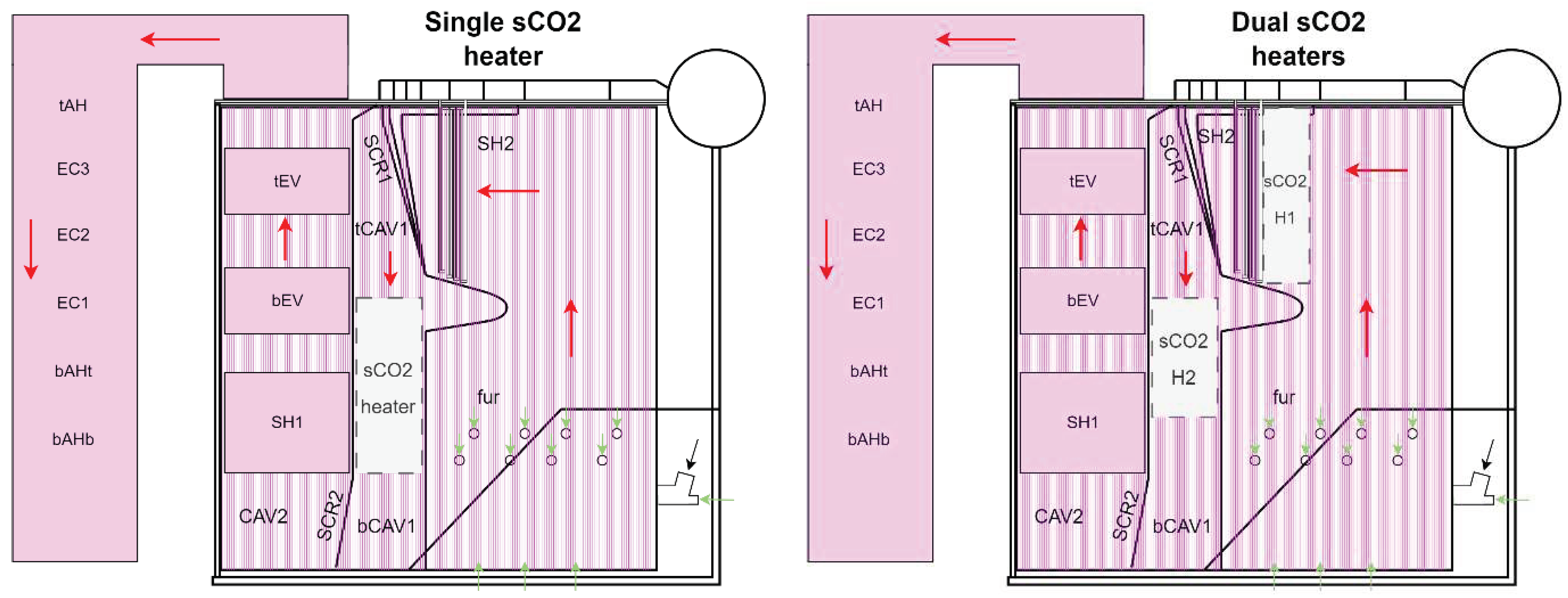
Figure 2. Process flow diagram for integrated cycle with single sCO2 heater.

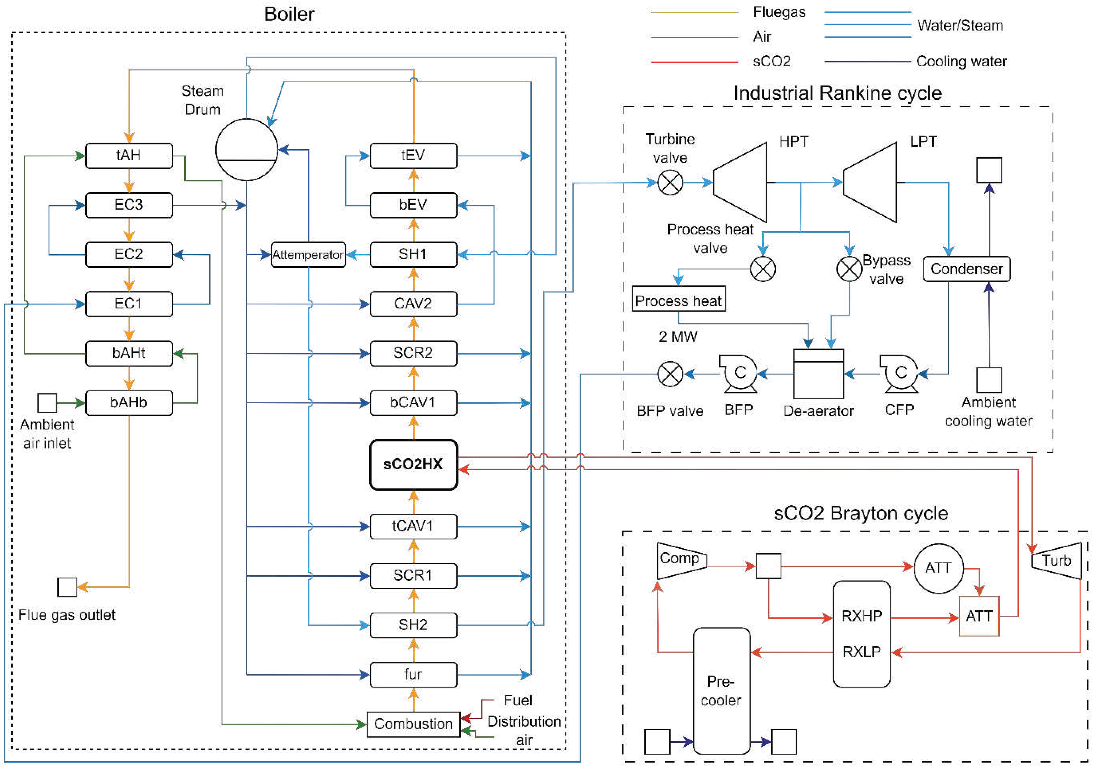
Figure 3. Process flow diagram for integrated cycle with dual sCO2 heaters.

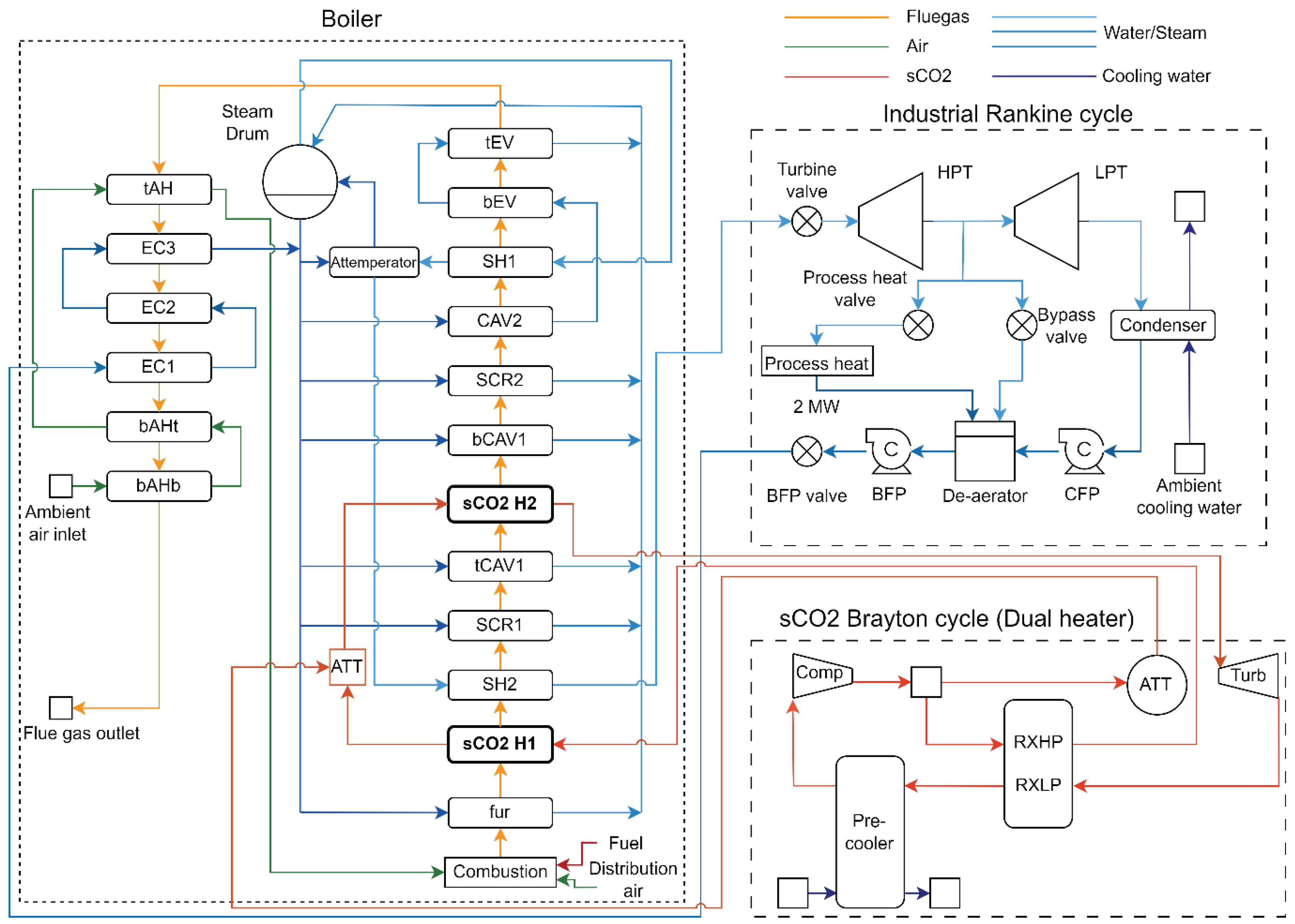
Figure 4. Radiative-convective heat exchanger modelling.

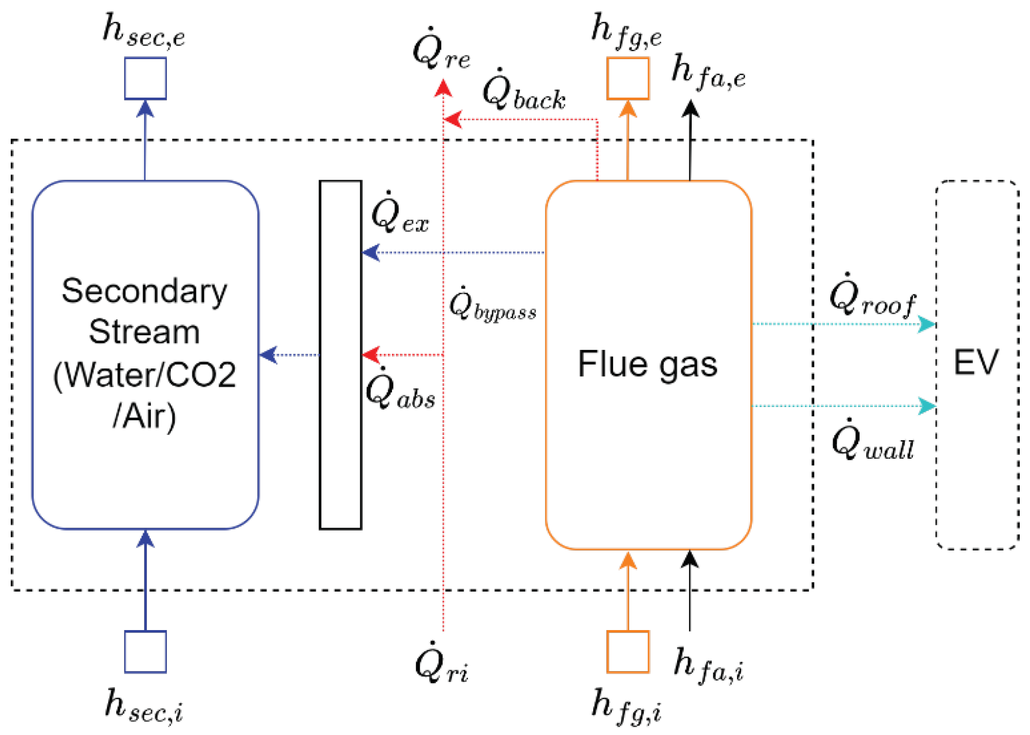
Figure 5. Thermal resistance network for radiative-convective heat exchanger tube bank.

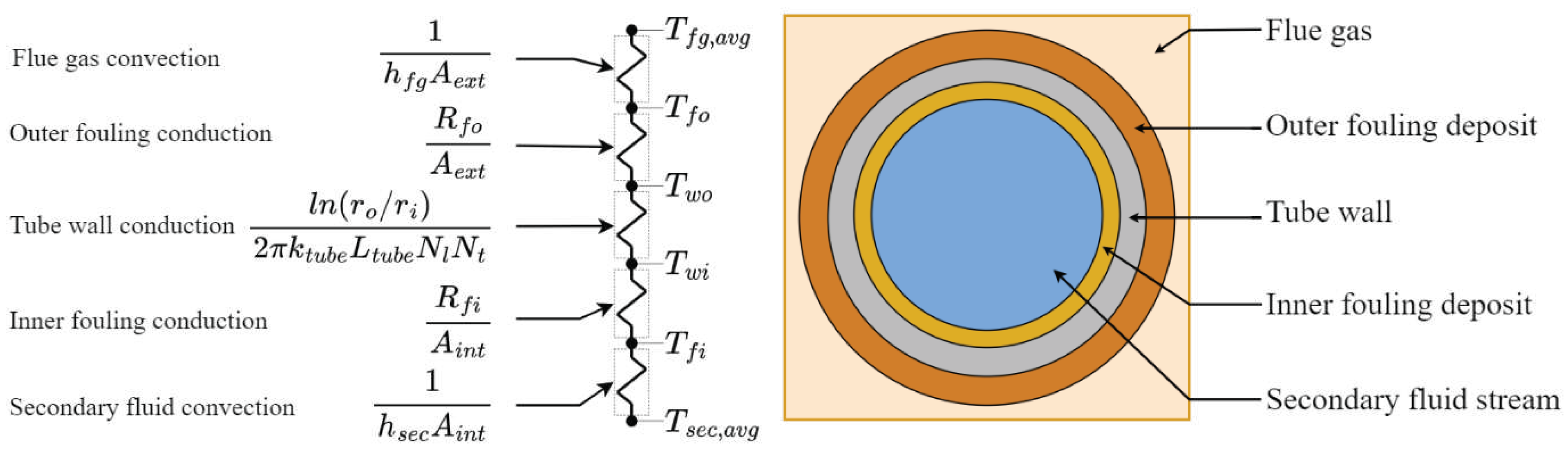
Figure 6. Inputs and boundary conditions for integrated cycle.

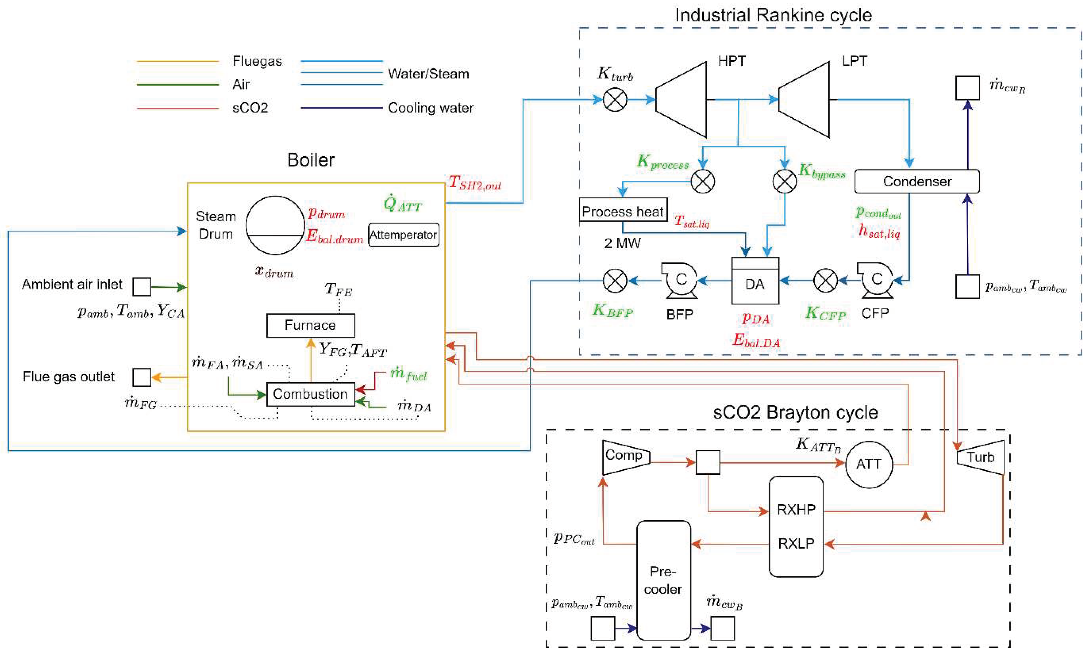
Figure 7. Rankine cycle T-s diagram.

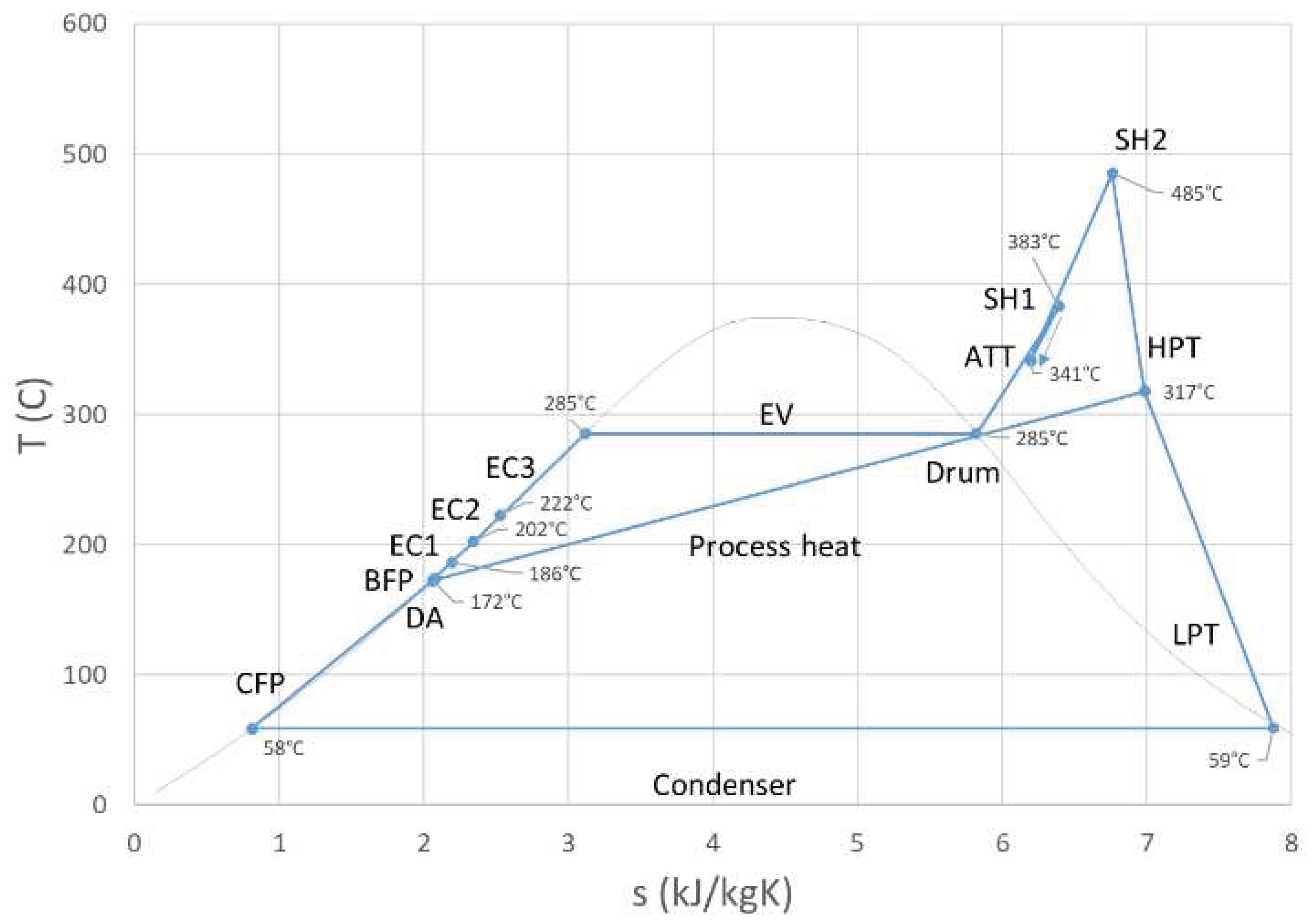
Figure 8. T-s diagram for TIT_Brayton= 550°C; Dual sCO2 heater config (top) and single sCO2 heater config (bottom).

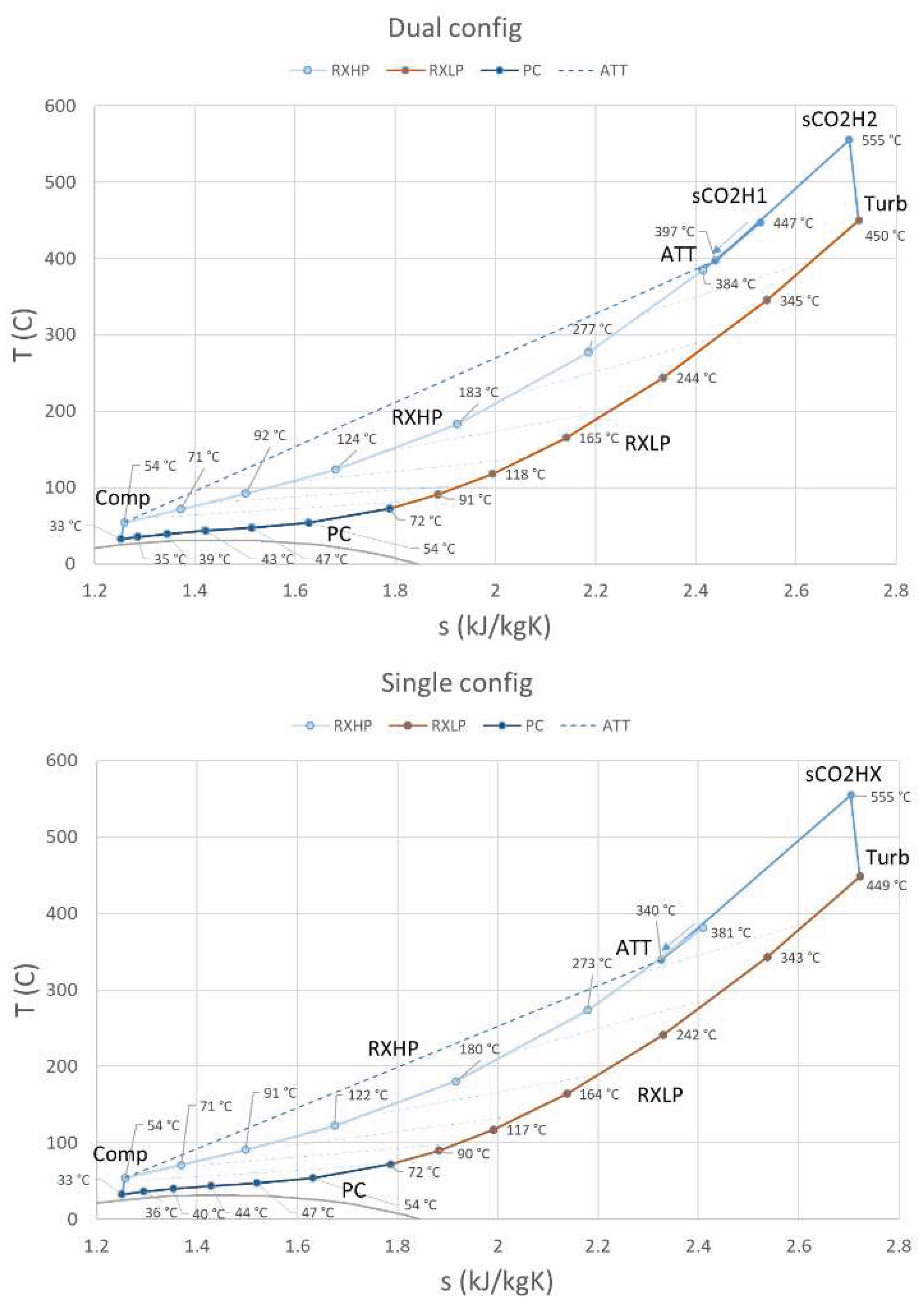
Figure 9. Flue gas heat transfer rate (loss) for existing, single, and dual configs (left). Relative difference to existing cycle (right).

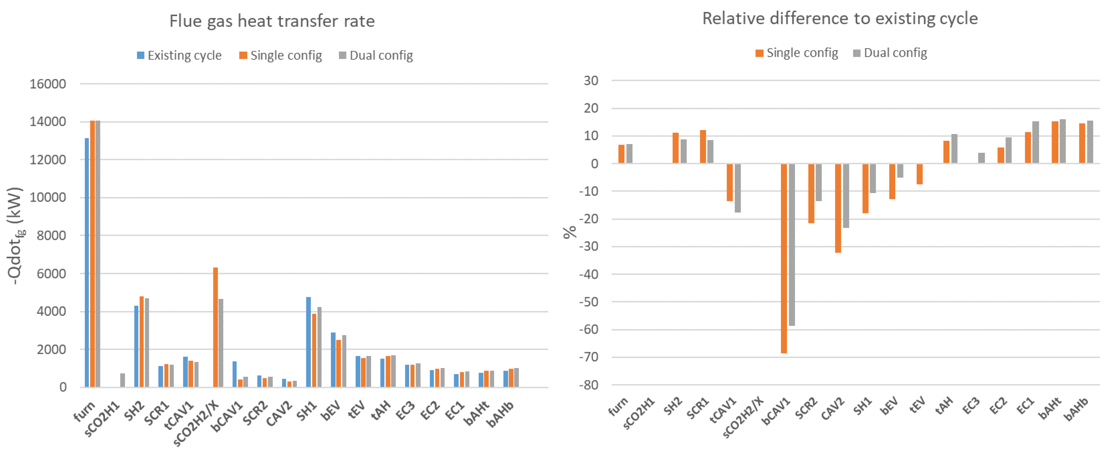
Figure 10. Heat transfer rates to water, sCO2, and air streams (left). Relative difference of Qdot _sec to existing cycle (right).

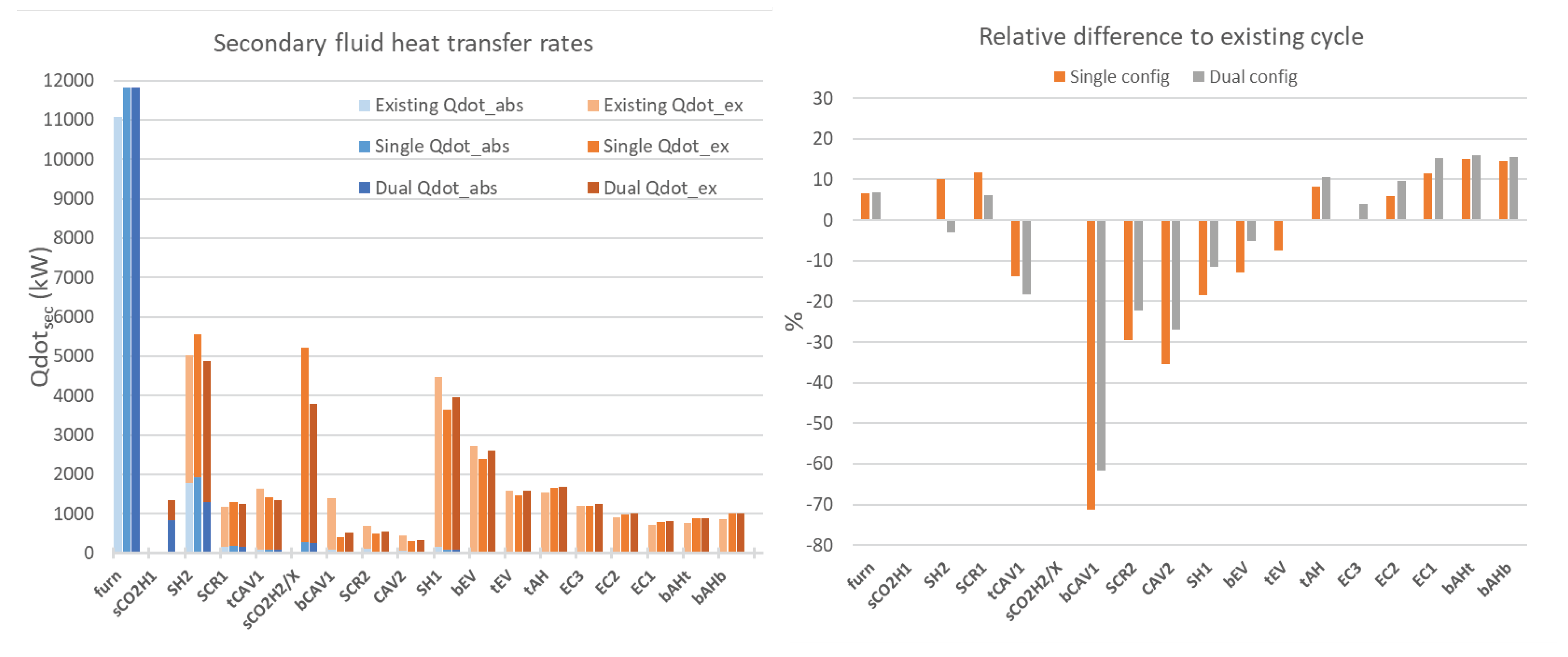
Figure 11. Average tube metal temperatures.

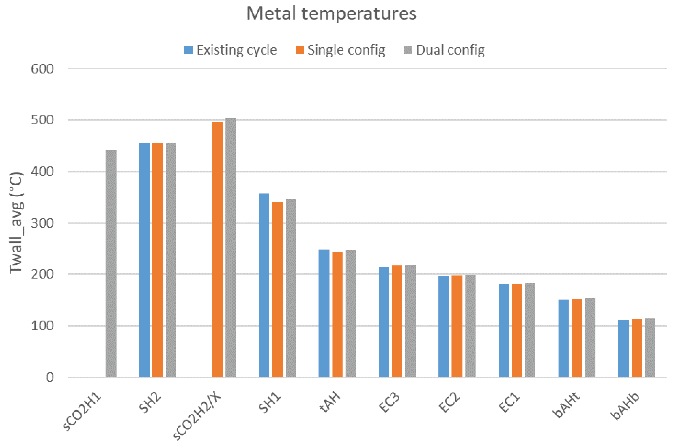
Table 1. Bagasse composition (as-received).

Fuel constituent	Carbon	Hydrogen	Oxygen	Nitrogen	Sulfur	Moisture	Ash	Unburnt carbon
Mass fraction (%)	21.09	2.68	20.77	0.16	0.02	50.0	4.66	0.62

Table 2. sCO2 heater specifications.

Single heater
	$W_{a v g}$ (m)	$H_{a v g}$ (m)	$L_{d u c t}$ (m)	$N_{t}$	$N_{l}$	$S_{t}$ (m)	$S_{l}$ (m)	$d_{O D}$ (m)	$t_{w a l l}$ (m)
sCO2HX	1.535	4.41	4.833	7	81	0.2	0.06	0.0381	0.00711
Dual heaters
sCO2H1	4.41	4.272	0.12	22	3	0.2	0.042	0.0381	0.00711
sCO2H2	1.535	4.41	3.40	7	43	0.2	0.08	0.0381	0.00711

Table 3. External control loop parameters, target functions, and constraints.

Controlled parameter	$p_{c o n d, o u t}$	$K_{C F P}$	$K_{p r o c e s s}$	$K_{b y p a s s}$
Target	Saturated liquid at condenser outlet	Mass balance over de-aerator	Energy balance for 2 MW process heat extraction	Energy balance at de-aerator
Constraint	$\begin{array}{l} h_{c o n d} = \\ h_{s a t, l i q} @ p_{c o n d} \end{array}$	$\begin{array}{l} p_{D A} = \\ 835 kPa \end{array}$	$\begin{array}{l} T_{p r o c e s s, e} = \\ T_{s a t, l i q} @ p_{p r o c e s s} \end{array}$	$\begin{array}{l} {\dot{m}}_{D A} h_{D A} = {\dot{m}}_{C F P} h_{C F P} \\ + {\dot{m}}_{H P T . b y p a s s} h_{H P T . b y p a s s} \\ + {\dot{m}}_{p r o c e s s . o u t} h_{p r o c e s s . o u t} \end{array}$
Controlled parameter	$K_{B F P}$	${\dot{m}}_{f u e l}$	${\dot{Q}}_{A T T}$
Target	Fixed pressure at steam drum	Energy balance at steam drum	Fixed temperature at SH2 outlet
Constraint	$\begin{array}{l} p_{S D} = \\ 6.914 MPa \end{array}$	$\begin{array}{l} {\dot{m}}_{S D} h_{S D} = {\dot{m}}_{E C 3. o u t} h_{E C 3. o u t} \\ + {\dot{m}}_{E V . o u t} h_{E V . o u t} \end{array}$	$\begin{array}{l} T_{S H 2, e} = \\ 485 ° C \end{array}$

Table 4. High level simulation results for the existing cycle, dual sCO2 heaters, and single sCO2 heater for TITs of 550°C, 650°C and 720°C.

		Fuel flow rate [kg/s]	Flue gas flow rate [kg/s]	${\dot{Q}}_{A T T_{R a n k i n e}}$ [kW]	sCO2 flow rate [kg/s]
	Existing cycle (no sCO2)	5.647	23.099	1580	-
550°C	Single sCO2 heater	6.512	26.636	1271	19.358
550°C	Dual sCO2 heaters	6.501	26.591	922	19.076
650°C	Single sCO2 heater	6.151	25.158	1331	10.577
650°C	Dual sCO2 heaters	6.149	25.153	1033	10.350
720°C	Single sCO2 heater	5.888	24.083	1373	4.970
720°C	Dual sCO2 heaters	5.979	24.454	1045	6.600
		sCO2 Brayton cycle net generation [kW]	$η_{t h . B r a y t o n}$ [%]	$η_{t h . O v e r a l l}$ [%]
	Existing cycle (no sCO2)	-	-	25.32
550°C	Single sCO2 heater	1861	35.68	26.66
550°C	Dual sCO2 heaters	1811	35.41	26.60
650°C	Single sCO2 heater	1221	40.37	26.50
650°C	Dual sCO2 heaters	1197	39.80	26.62
720°C	Single sCO2 heater	627.9	42.34	26.00
720°C	Dual sCO2 heaters	833.2	41.66	26.19

Table 5. Rankine cycle results for all configurations.

	Feedwater flow rate [kg/s]	Condenser pressure [kPa]	Rankine cycle net generation [kW]	$η_{t h . R a n k i n e}$ [%]
All cycle configurations	13.127	18.3	8760	25.30%

Table 6. Outlet temperatures at RXHP, sCO2H1, and ATT for dual and single heater configuration.

	$T_{R X H P_{o u t}} [° C]$	$T_{s C O 2 H 1_{o u t}} [° C]$	$T_{A T T_{o u t}} [° C]$
Single config	381	-	340
Dual config	384	447	397

Table 7. Furnace heat uptake breakdown.

	${\dot{Q}}_{F E} [kW]$	${\dot{Q}}_{W W} [kW]$	${\dot{Q}}_{R F} [kW]$	${\dot{Q}}_{l o s s . f u r} [kW]$	${\dot{Q}}_{f g . f u r} (Tot) [kW]$
Existing	1940	10865	210	133	-13148
Single	2091	11588	226	142	-14047
Dual	2094	11603	226	142	-14065

Table 8. Boiler heat load breakdown for existing cycle, single configuration, dual configuration.

		Existing (kW)	Single (kW)	Dual (kW)	Existing %	Single %	Dual %
EC	EC1	715	797	824	25.2	26.8	26.8
	EC2	922	975	1010	32.5	32.8	32.8
	EC3	1199	1201	1246	42.3	40.4	40.5
		2836	2973	3080		(+4.8%)	(+8.6%)

EV	furn	11075	11814	11830	46.4	49.8	50.1
	bEV	2897	2522	2746	12.1	10.6	11.6
	tEV	1665	1540	1667	6.97	6.49	7.06
	Other	8251	7853	7382	34.5	33.1	31.2
		23889	23729	23626

SH	SH1	4462	3634	3950	56.4	46.0	50.0
	ATT	-1580	-1271	-922	-20.0	-16.1	-11.7
	SH2	5030	5543	4879	63.6	70.1	61.7
		7912	7906	7907
Total		34637	34608	34612

sCO2	sCO2H1	-	-	1336	-	-	26.1
	sCO2H2/X	-	5215	3778	-	100	73.9
			5215	5114

${\dot{Q}}_{T o t}$		34637	39823	39726
$η_{b o i l e r}$ (%)		64.36	64.32	64.18

Disclaimer/Publisher’s Note: The statements, opinions and data contained in all publications are solely those of the individual author(s) and contributor(s) and not of MDPI and/or the editor(s). MDPI and/or the editor(s) disclaim responsibility for any injury to people or property resulting from any ideas, methods, instructions or products referred to in the content.

© 2024 by the authors. Licensee MDPI, Basel, Switzerland. This article is an open access article distributed under the terms and conditions of the Creative Commons Attribution (CC BY) license (https://creativecommons.org/licenses/by/4.0/).

Copyright: This open access article is published under a Creative Commons CC BY 4.0 license, which permit the free download, distribution, and reuse, provided that the author and preprint are cited in any reuse.

MDPI Initiatives

Important Links

Choose an area of interest and we will send you notifications of new preprints at your preferred frequency.

Disclaimer

Integrated Performance of a Modular Biomass Boiler with a Combined Heat and Power Industrial Rankine Cycle and Supplementary sCO2 Brayton Cycle

Abstract

1. Introduction

2. Cycle Layout and Operation

3. Thermofluid Network Model

3.1. Boiler

3.1.1. Combustion

3.1.2. Furnace

3.1.3. Boiler Heat Exchangers

3.2. Rankine Cycle

3.3. Brayton Cycle

3.4. Boundary Conditions, Set Points, and Solution Procedure

4. Results and Discussion

4.1. Rankine Cycle

4.3. Boiler Heat Exchangers

4.3.1. Flue Gas Heat Transfer Rates and Temperatures

4.3.2. Water/sCO2/Air Temperatures and Heat Transfer

4.3.3. Tube Metal Temperatures

4.4. Boiler Heat Load Breakdown

5. Conclusions

Acknowledgments

Nomenclature

References

MDPI Initiatives

Important Links

Subscribe

Integrated Performance of a Modular Biomass Boiler with a Combined Heat and Power Industrial Rankine Cycle and Supplementary sCO₂ Brayton Cycle